Abstract

We say that a chessboard filled with integer entries satisfies the neighbour-sum property if the number appearing on each cell is the sum of entries in its neighbouring cells, where neighbours are cells sharing a common edge or vertex. We show that an $n\times n$ chessboard satisfies this property if and only if $n\equiv 5\pmod{6}$. Existence of solutions is further investigated of rectangular, toroidal boards, as well as on Neumann neighbourhoods, including a nice connection to discrete harmonic functions. Construction of solutions on infinite boards are also presented. Finally, answers to three dimensional analogues of these boards are explored using properties of cyclotomic polynomials and relevant ideas conjectured.

key-words: p-adic valuation, Kronecker product, spatial lattice, discrete harmonic function, cyclotomic polynomials

1 Introduction

The Regional Mathematical Olympiad (RMO) is the second of a series of math tests held in India, which all leads up to participation in the International Mathematical Olympiad (IMO).

Our inspiration stems from RMO 1991 Problem 8 -

The 64 squares of an 8 × 8 chessboard are filled with positive integers in such a way that each integer is the average of the integers on the neighbouring squares. (Two squares are neighbours if they share a common edge or a common vertex. Thus a square can have 8, 5 or 3 neighbours depending on its position). Show that all the 64 integer entries are in fact equal.

Brief Solution: Any given entry must lie in between the smallest and largest entries of its neighbours. Thus, the largest entry on the board must be surrounded by identical entries. This forces all entries to be equal.

While this has a surprisingly bleak answer, a small modification to the criterion might not be so! This is the analogue we explore in this paper:

An $n\times n$ chessboard for $n\geq 3$, with each square bearing an integer, is said to have the neighbour-sum property if each number is the sum of the numbers on the neighbouring squares (Such a collection of elements is called a solution). Two squares are neighbours if they share a common edge or a common vertex. A chessboard with all squares bearing the number zero is said to be a trivial solution.

For an $n\times n$ chessboard, how many distinct non-trivial solutions are there?

At a first glance, the problem might seem to be rooted in combinatorics, but certain observations favour a different angle. It is clear that given a non-trivial solution $((x_{ij}))$ of the matrix representation $X$ of a chessboard (of dimension $n\times n$ for some $n$), all matrix representations of the form $\alpha X=((\alpha x_{ij})),\;\alpha\in\mathbb{Z}\backslash\{0\}$ are also valid non-trivial solutions. Furthermore, sum of two solutions is also another solution. This motivates the idea of a transformation which contains the vectorisation [6] of $X$ in its kernel.

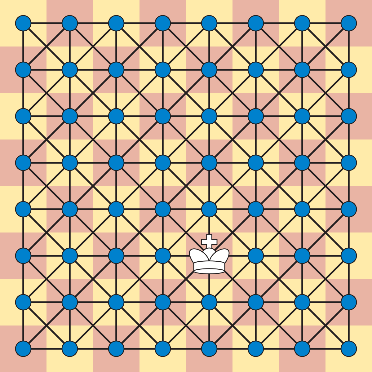
Figure 1: King’s Graph on a standard $8\times 8$ chessboard. Image Courtesy: David Epstein

2 Finding square boards with such solutions

Trying to resolve our problem has led us to a critical observation - sum of solutions is a solution. It remains to produce an appropriate transformation $T$ such that for a chessboard $\symking\in M_{n}(\mathbb{Z})$ (the use of this notation being a subtle foreshadowing) with its vectorisation $\bm{\operatorname{vec}(\symking)}\in\mathbb{Z}^{n^{2}}$, one has

$$T\bm{\operatorname{vec}(\symking)}=\bm{0}$$

An immediate transformation is one that replaces every element with the sum of its neighbours minus the element itself. Clearly, all solutions would be in the kernel of this transformation. For a $2\times 2$ chessboard,

$$\symking_{2\times 2}=\begin{array}[]{|c|c|}\hline\cr x_{1}&x_{3}\\ \hline\cr x_{2}&x_{4}\\ \hline\cr\end{array}$$

the corresponding $4\times 4$ transformation would be given by

$$T_{4\times 4}=\begin{pmatrix}-1&1&1&1\\ 1&-1&1&1\\ 1&1&-1&1\\ 1&1&1&-1\end{pmatrix}$$

This is non-singular, so this does not have a non-trivial kernel. Note that we are only interested in $n\geq 3$, and the same can be shown for $T_{3\times 3}$ for $n=3$. But are there some values of $n$ for which non-trivial solutions can be present? This takes us to our main result.

2.1 Existence of solutions

Theorem 1.

An $n\times n$ chessboard has a non-trivial solution of the neighbour-sum property if and only if $6\mid(n+1)$.

This is a very specific result, and to prove it we will first have to introduce some key ideas.

Let $\symking$ be an $n\times n$ chessboard, and let $T_{n}$ be the transformation mentioned above. Then, one can write $A_{n}=T_{n}+\mathbb{I}_{n^{2}}$, where $A_{n}$ is precisely the adjacency matrix of the square chessboard where adjacency is only amongst neighbours. Denote the $i$-th element of $\bm{\operatorname{vec}(\symking)}$ as $\symking_{i}$. Then, the $i$-th entry of the vector $A_{n}\bm{\operatorname{vec}{\symking}}$ gives the sum of the neighbours of the square $\symking_{i}$. This means that the neighbour-sum property can be expressed as $A_{n}\bm{\operatorname{vec}\symking}=\bm{\operatorname{vec}{\symking}}$.

Proposition 2.

The set of all vectorised solutions is in $\ker(T_{n})$, which always contains the trivial solution.

Proposition 3.

Define $B_{n}\in M_{n}(\mathbb{Z})$ with $B_{ij}=1$ when $|i-j|\leq 1$ and $B_{ij}=0$ otherwise. Then,

$$A_{n}=B_{n}\otimes B_{n}-\mathbb{I}_{n^{2}},\qquad T_{n}=B_{n}\otimes B_{n}-2\mathbb{I}_{n^{2}}.$$

Proof.

Note that $B_{n}$ can be interpreted as the adjacency matrix ([2], pg. 7) of a graph $G_{n}$ on vertices $\{1,\dots,n\}$, where $i,i^{\prime}$ are neighbours when $|i-i^{\prime}|\leq 1$. In the Cartesian product ([8], pg. 115 - 116) $G_{n}\times G_{n}$, whose adjacency matrix is $B_{n}\otimes B_{n}$, we have an edge between $(i,j)$ and $(i^{\prime},j^{\prime})$ precisely when $|i-i^{\prime}|\leq 1$ and $|j-j^{\prime}|\leq 1$. Removing self loops by subtracting $\mathbb{I}_{n^{2}}$ from the adjacency matrix yields the transformation $A_{n}$ as desired.         ∎

Remark. The graph $G_{n,n}$ is called the King’s Graph [3, 1], because it shows the movement of a King on a chessboard. At any square (equivalent to a node in the graph), the King has 3,5 or 8 adjacent squares to move to depending on its position on the board. The adjacency matrix of this graph is $A_{n}=B_{n}\otimes B_{n}-\mathbb{I}_{n^{2}}$. This implicit relation is the solitary reason for the $\symking$ notation.

$$B_{5}=\begin{bmatrix}1&1&0&0&0\\ 1&1&1&0&0\\ 0&1&1&1&0\\ 0&0&1&1&1\\ 0&0&0&1&1\end{bmatrix},\qquad B_{5}\otimes B_{5}=\begin{bmatrix}B_{5}&B_{5}&0&0&0\\ B_{5}&B_{5}&B_{5}&0&0\\ 0&B_{5}&B_{5}&B_{5}&0\\ 0&0&B_{5}&B_{5}&B_{5}\\ 0&0&0&B_{5}&B_{5}\end{bmatrix}$$

With this, our search for non-trivial chessboards with the neighbour-sum property reduces to finding eigenvectors of $B_{n}\otimes B_{n}$ corresponding to the eigenvalue $2$.

Fact 4.

The eigenvalues of $A\otimes B$ are $\{\lambda_{i}\mu_{j}\}$, where $\{\lambda_{i}\}$ are the eigenvalues of $A$, and $\{\mu_{j}\}$ are the eigenvalues of $B$ [11].

Fact 5.

The eigenvalues of $B_{n}$ are $\lambda_{k}=1+2\cos(k\pi/(n+1))$ for $k=1,\dots,n$. This is due to the tridiagonal Toeplitz form of $B_{n}$ with all non-zero elements being unity [13].

Using these two facts, we formulate the following proposition.

Proposition 6.

The space $\ker(T_{n})$ is non-trivial if and only if there exist $p,q\in\mathbb{N}$ such that $1\leq p,q\leq n$ and

$$\left(1+2\cos\left(\frac{p\pi}{n+1}\right)\right)\left(1+2\cos\left(\frac{q\pi}{n+1}\right)\right)=2.$$

In order to deal with the equation in Proposition (6) and others similar to it, we require the following result.

Theorem 7.

The only solutions of

$$\left(1+2\cos(u\pi)\right)\left(1+2\cos(v\pi)\right)=2.$$

where $u,v\in\mathbb{Q}\cap(0,1)$ are $u=1/3,v=1/2$ and $u=1/2,v=1/3$.

Proof of Theorem 7.

The given equation can be rewritten as

$$(\alpha+1+\alpha^{-1})(\beta+1+\beta^{-1})=2,$$ (1)

where $\alpha=e^{iu\pi},\beta=e^{iv\pi}$ are roots of unity with positive imaginary parts.

Let $u=p/N$, $v=q/N$ be a solution of this equation, where $p,q,N\in\mathbb{N}$ and $1\leq p,q<N$. Set $R=\mathbb{Z}[e^{\pi i/N}]$. Let $\mathfrak{p}$ be a prime of $R$ lying over the prime $2$ in $\mathbb{Z}$, and let $v:R\to\mathbb{Q}$ be the $\mathfrak{p}$-adic valuation ([7] pg. 755), normalized so that $v(2)=1$. So, Equation 1 gives

$$v(\alpha+1+\alpha^{-1})+v(\beta+1+\beta^{-1})=1.$$ (2)

To proceed any further, we state the following lemma.

Lemma 8.

Let $\eta$ be a primitive $m$-th root of unity. Then

$$v(\eta+1+\eta^{-1})=\begin{cases}\infty&m=3\\ 1/2^{k}&m=3\cdot 2^{k+1}\ \text{for}\ k\geq 0\\ 0&\text{otherwise}\end{cases}.$$

Now, it is clear that the only ways to decompose $1$ as a sum of two numbers in $\{\infty,1,1/2,1/4,\cdots,0\}$ are $1+0$, $0+1$ and $1/2+1/2$. We use this in Equation 2.

Case I: If $v(\alpha+1+\alpha^{-1})=1$, $v(\beta+1+\beta^{-1})=0$, then $\alpha$ must be a primitive $6$-th root of unity, forcing $\alpha=e^{i\pi/3}$, $u=1/3$. This in turn forces $v=1/2$. Interchanging the roles of $\alpha,\beta$ yields the solution $u=1/2$, $v=1/3$.

Case II: If $v(\alpha+1+\alpha^{-1})=v(\beta+1+\beta^{-1})=1/2$, then $\alpha,\beta$ must be primitive $12$-th roots of unity, forcing $\alpha,\beta\in\{e^{i\pi/6},e^{5i\pi/6}\}$. This gives, $\alpha+1+\alpha^{-1},\beta+1+\beta^{-1}\in\{1+\sqrt{3},1-\sqrt{3}\}$; but these do not satisfy Equation 1.         ∎

Now, we return to the proof of the Lemma we just used.

Proof of Lemma 8.

The case $\eta=1$ (so $m=1$) is easy to check by hand, so we assume that $\eta\neq 1$ from now on.

We have

$$\eta+1+\eta^{-1}=\eta^{-1}\cdot\frac{\eta^{3}-1}{\eta-1}$$

so

$$v(\eta+1+\eta^{-1})=v(\eta^{3}-1)-v(\eta-1).$$

Now, if $\omega$ is a primitive $\ell$-th root of unity, then

$$v(\omega-1)=\begin{cases}\infty&\ell=1\\ 1/2^{k}&\ell=2^{k+1}\\ 0&\text{otherwise}\end{cases}$$

as, if $\ell=1$, then $\zeta_{\ell}-1=0$; if two distinct primes divide $\ell$, then $1-\zeta_{\ell}$ is a unit; and if $\ell=p^{k}$, then we have $(\zeta_{\ell}-1)^{\phi(\ell)}=(p)$ as ideal and hence, $v(\zeta_{\ell}-1)$ is nonzero only when $p=2$ and the valuation is $\frac{1}{\phi(\ell)}$.

Since $\eta$ is a primitive $m$-th root of unity, $\eta^{3}$ is a primitive $m/\text{GCD}(m,3)$-th root of unity, so combining the above two equations gives the claim.         ∎

Finally, we are equipped with enough tools to provide a proof for Theorem 1.

Proof of Theorem 1.

Propositions (2) and (6) give a criterion for the existence of non-trivial $n\times n$ chessboards with the neighbour-sum property. Theorem (7) forces both $2\mid(n+1)$ and $3\mid(n+1)$, from which the claim follows.         ∎

2.2 Looking at the solutions

If the dimension $n$ of a square board is one less than a multiple of 6, the transformation $B_{n}\otimes B_{n}$ has eigenvalue $2$ with multiplicity $2$, which implies that $\ker(T_{n})$ is two-dimensional. It is a matter of computation to yield the exact solutions, which correspond to the associated eigenvectors. For the smallest board satisfying the neighbour-sum property ($n=5$),

$$\symking^{(1)}_{5\times 5}=\begin{array}[]{|c|c|c|c|c|}\hline\cr 1&0&-1&0&1\\ \hline\cr 1&0&-1&0&1\\ \hline\cr\phantom{-}0\phantom{-}&\phantom{-}0\phantom{-}&\phantom{-}0\phantom{-}&\phantom{-}0\phantom{-}&\phantom{-}0\phantom{-}\\ \hline\cr-1&0&1&0&-1\\ \hline\cr-1&0&1&0&-1\\ \hline\cr\end{array}\qquad\text{and}\qquad\symking^{(2)}_{5\times 5}=\begin{array}[]{|c|c|c|c|c|}\hline\cr 1&1&0&-1&-1\\ \hline\cr\phantom{-}0\phantom{-}&\phantom{-}0\phantom{-}&\phantom{-}0\phantom{-}&\phantom{-}0\phantom{-}&\phantom{-}0\phantom{-}\\ \hline\cr-1&-1&0&1&1\\ \hline\cr 0&0&0&0&0\\ \hline\cr 1&1&0&-1&-1\\ \hline\cr\end{array}$$

are the only solutions.

Clearly, these solutions are the transposes of each other, considered distinct due to their vectorisations being so. These are surprisingly simple solutions, with every element being in the set $\{-1,0,1\}$. Custom solutions can be produced with linear combinations $\lambda\symking^{(1)}_{5\times 5}+\mu\symking^{(2)}_{5\times 5}$ for $\lambda,\mu\in\mathbb{Z}$, both not zero.

One observation is critical in understanding the kind of solutions one should expect to see for larger square boards admitting solutions. Define a phantom boundary to be a boundary of cells (all containing zero) of a board such that the elements of the boundary contribute only to the neighbour-sum property of the board and not themselves.

Consider the following $2\times 2$ board with a phantom boundary (represented in yellow), yielding a $4\times 4$ board.

$$\begin{array}[]{|c|c|c|c|}\hline\cr 0&0&0&0\\ \hline\cr\pagecolor[HTML]{F7F978}0&x_{1}&x_{3}&\pagecolor[HTML]{F7F978}0\\ \hline\cr\pagecolor[HTML]{F7F978}0&x_{2}&x_{4}&\pagecolor[HTML]{F7F978}0\\ \hline\cr 0&0&0&0\\ \hline\cr\end{array}$$

The presence of the phantom boundary does not alter the conditions necessary for the $2\times 2$ to satisfy the neighbour-sum property as the zeroes don’t contribute to the sum. This idea is key to be able to identify disjoint solutions in large boards.

We can already see that the $5\times 5$ solutions can be formed of small $2\times 1$ units, emphasized in the following figure.

$$\symking^{(1)}_{5\times 5}=\begin{array}[]{|c|c|c|c|c|}\hline\cr\pagecolor[HTML]{F7F978}1&0&\pagecolor[HTML]{F7F978}-1&0&\pagecolor[HTML]{F7F978}1\\ \hline\cr\pagecolor[HTML]{F7F978}1&0&\pagecolor[HTML]{F7F978}-1&0&\pagecolor[HTML]{F7F978}1\\ \hline\cr\phantom{-}0\phantom{-}&\phantom{-}0\phantom{-}&\phantom{-}0\phantom{-}&\phantom{-}0\phantom{-}&\phantom{-}0\phantom{-}\\ \hline\cr\pagecolor[HTML]{F7F978}-1&0&\pagecolor[HTML]{F7F978}1&0&\pagecolor[HTML]{F7F978}-1\\ \hline\cr\pagecolor[HTML]{F7F978}-1&0&\pagecolor[HTML]{F7F978}1&0&\pagecolor[HTML]{F7F978}-1\\ \hline\cr\end{array}$$

Adding a phantom boundary to this solution clearly shows that the solution can 6 disjoint regions (three $(1,1)$ and three $(-1,-1)$, alternating) separated by zeroes. This pattern can easily be repeated to get the two solutions for $n=11,17,\ldots$. Since the kernel is always 2 dimensional, the solutions on $n\times n$ formed from extensions of those on $5\times 5$ form a basis for the eigenspace. This gives us a complete characterization of solutions of the neighbour-sum property on square boards.

It is easy to see and prove that in the standard solutions, every second column and third row in $\symking_{n\times n}^{(1)}$ (resp. second row and third column in $\symking^{(2)}_{n\times n}$) contains only zero elements. The only zeroes that are common are at positions $(i,j)$ where either both $i$ and $j$ are even or they are both multiples of 3. So, any non-trivial linear combination $\lambda\symking^{(1)}_{5\times 5}+\mu\symking^{(2)}_{5\times 5}$ for $\lambda,\mu\in\mathbb{Z}$ would preserve the zeroes in those positions.

Remark. As the standard solutions form a basis for the kernel, there cannot be any square board with a non-trivial solution without any zero elements.

3 Lessening symmetry - from squares to rectangles

A simple generalization of the neighbour-sum property can be made to rectangular boards of size $m\times n$ with $m,n\geq 2$. Theorem 7 will still be key to finding solutions here.

Following similar arguments as in the case of $n\times n$ chessboards, it is not difficult to arrive at analogues of Propositions 3 and 6 for $m\times n$ chessboards.

Proposition 9.

The set of all $m\times n$ solutions i.e., $m\times n$ chessboards with the neighbour-sum property, is in $\ker(T_{m,n})$, where

$$T_{m,n}=B_{m}\otimes B_{n}-2\mathbb{I}_{mn}.$$

Proposition 10.

The space $\ker(T_{m,n})$ is non-trivial if and only if there exist $p,q\in\mathbb{N}$ such that $1\leq p\leq m$, $1\leq q\leq n$ and

$$\left(1+2\cos\left(\frac{p\pi}{m+1}\right)\right)\left(1+2\cos\left(\frac{q\pi}{n+1}\right)\right)=2.$$

This yields the following characterisation.

Theorem 11.

Non-trivial $m\times n$ chessboards satisfying the neighbour-sum property exist if and only if $2\mid(m+1)$ and $3\mid(n+1)$, or vice versa.

Proof.

Follows immediately from Proposition 10 and Theorem 7.

∎

Remark. The dimension of $\ker(T_{m,n})$ is at most $2$. It is equal to $1$ only if $m\neq n$.

This remark follows directly from the solution space explored before. There are two fundamental solutions for a square board, and they can only fit in a rectangular board if both dimensions are large enough. In all other cases, we have the nullity to be at most $1$.

Some simple consequences of these are:

1. If $\symking_{m\times n}$ has a non-trivial kernel of dimension $d\leq 2$, then $\symking_{n\times m}$ also has a non-trivial kernel of dimension $d$. Further, the solutions are transposes of one-another.

2. The standard solutions of a square board can be partitioned into disjoint non-trivial rectangular solutions.

3. A chessboard of dimensions $m\times n$, where $m+1$ is even and $n+1$ is an odd multiple of 3 (or vice versa), has solution(s) by Theorem 11. Then, a board of dimensions $(m+1)\times(n+1)$ also has solution(s). Furthermore, if a standard solution of the $m\times n$ board is made of $2\times 1$ units, then a corresponding standard solution on the $(m+1)\times(n+1)$ board is made of similar $1\times 2$ units. This correspondence is clear when $ker(T_{m,n})$ has dimension $1$.

4 Coffee Mugs

For any finite board, a plethora of boundary effects come into being while deducing solutions for the neighbour-sum property. Which already prompts a natural curiosity - what if there were no boundaries? And where else to look for but a good old coffee mug a.k.a a torus!

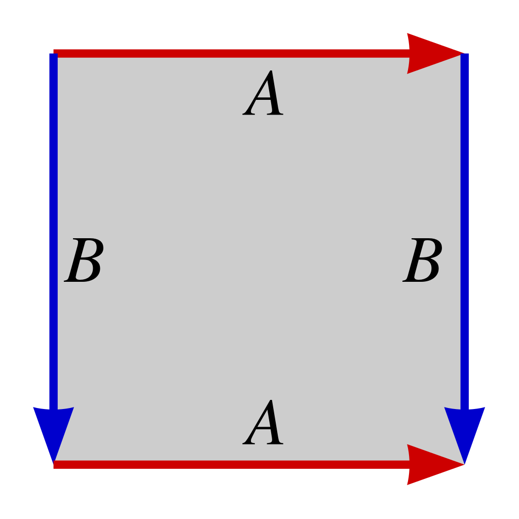
Figure 2: A torus is formed from a square/rectangle by gluing opposite sides, which makes the rectangle a fundamental polygon of the torus. Image Courtesy: Ilmari Karonen, Wikimedia Commons

Simply speaking, a Torus in $\mathbb{R}^{3}$ is just the Cartesian product of two circles, given by $\mathbb{T}^{2}=\mathbb{S}^{1}\times\mathbb{S}^{1}$ ([9], pg. 5). In our case, we can form one from a rectangular $m\times n$ board $X$ by wrapping around the board along the two dimensions. We must first define an appropriate adjacency matrix $A_{m,n}^{\circ}$ which endows $X$ with the correct neighbourhood structure. Following that, we set $T_{m,n}^{\circ}=A_{m,n}^{\circ}-\mathbb{I}_{mn}$ and examine the solution space $\ker(T_{m,n}^{\circ})$.

4.1 Solutions on Coffee Mugs

Proposition 12.

Define $B_{n}^{\circ}\in M_{n}(\mathbb{Z})$ with $B_{ij}^{\circ}=1$ when $i-j\in\{-1,0,1\}\pmod{n}$ and $B_{ij}^{\circ}=0$ otherwise. Then,

$$A_{m,n}^{\circ}=B_{m}^{\circ}\otimes B_{n}^{\circ}-\mathbb{I}_{mn},\qquad T_{m,n}^{\circ}=B_{m}^{\circ}\otimes B_{n}^{\circ}-2\mathbb{I}_{mn}.$$

Proof.

Note that $B_{n}^{\circ}$ is the adjacency matrix of the graph $G_{n}$ from Proposition 3 with the extra edge $(n,1)$. Proceeding in the same manner, we obtain the required adjacency matrix of the toroidal King’s Graph $G_{m,n}^{\circ}$.         ∎

Fact 13.

The eigenvalues of $B_{n}^{\circ}$ are $\lambda_{k}^{\circ}=1+2\cos(2k\pi/n)$ for $k=1,\dots,n$. [13]

Note that $B_{n}^{\circ}$ is a tridiagonal circulant matrix [5] with all non-zero entries being unity, wherefore its eigenvalues are solutions to its associated polynomial $f(x)=1+x+x^{n-1}$, which gives the above result.

Proposition 14.

The space $\ker(T_{m,n}^{\circ})$ is non-trivial if and only if there exist $p,q\in\mathbb{N}$ such that $1\leq p\leq m$, $1\leq q\leq n$ and

$$\left(1+2\cos\left(\frac{2p\pi}{m}\right)\right)\left(1+2\cos\left(\frac{2q\pi}{n}\right)\right)=2.$$

Theorem 15.

Non-trivial $m\times n$ toroidal chessboards satisfying the neighbour-sum property exist if and only if $4\mid m$ and $6\mid n$, or vice versa.

Proof.

Follows from Proposition 14 and Theorem 7. Note that the edge cases where $p=m/2$ or $p=m$ can be eliminated by hand.         ∎

5 The Neumann Neighbourhood

Working with a spatial lattice yields some nice analogues, such as torii. Anither way to generate analogues is by redefining the idea of neighbours. We would take a look at the Neumann neighbourhood [16] in this section. An $n\times n$ chessboard for $n\geq 3$, with each square bearing an integer, is said to have the Neumann-neighbour-sum (Nns) property if each number is the sum of the numbers on the neighbouring squares - where two squares are neighbours if and only if they share a common edge. Solutions and trivial solutions are defined as before.

Are there non-trivial boards with Nns property?

5.1 On Existence

Proposition 16.

The set of all $m\times n$ chessboards with the Neumann-neighbour-sum property is in $\ker(T_{m,n}^{+})$, where

$$T_{m,n}^{+}=B_{m}\oplus B_{n}-3\mathbb{I}_{mn}=B_{m}\otimes\mathbb{I}_{n}+\mathbb{I}_{m}\otimes B_{n}-3\mathbb{I}_{mn}.$$

Proof.

Let $G_{m,n}^{+}$ be the graph corresponding to an $m\times n$ chessboard with the Neumann neighbourhood structure. We claim that its adjacency matrix is

$$A_{m,n}^{+}=B_{m}\otimes\mathbb{I}_{n}+\mathbb{I}_{m}\otimes B_{n}-2\mathbb{I}_{mn}.$$

Indeed, in the graph corresponding to the adjacency matrix $B_{m}\otimes\mathbb{I}_{n}$, each square is connected to itself and the squares above and below it. Similarly, in the graph corresponding to $\mathbb{I}_{m}\otimes B_{n}$, each square is connected to itself and the squares to its left and right. Adding these two graphs gives $G_{m,n}^{+}$ except with two self loops for each square, which we remove by subtracting $2\mathbb{I}_{mn}$ to retrieve the above expression for $A_{m,n}^{+}$.         ∎

Fact 17.

The eigenvalues of $A\oplus B$ are $\{\lambda_{i}+\mu_{j}\}$, where $\{\lambda_{i}\}$ are the eigenvalues of $A$, and $\{\mu_{j}\}$ are the eigenvalues of $B$ [11].

This gives us an eigenvalue equation unlike those we’ve seen so far.

Proposition 18.

The space $\ker(T_{m,n}^{+})$ is non-trivial if and only if there exist $p,q\in\mathbb{N}$ such that $1\leq p\leq m$, $1\leq q\leq n$ and

$$\cos\left(\frac{p\pi}{m+1}\right)+\cos\left(\frac{q\pi}{n+1}\right)=\frac{1}{2}.$$

Now we discuss a particular case $m=n$. We want solutions of $2\cos\left(\frac{a\pi}{n+1}\right)+2\cos\left(\frac{b\pi}{n+1}\right)=1$ with $a,b\in\{1,2,3,\ldots,n\}$.

Theorem 19.

[4] Suppose we have at most four distinct rational multiples of $\pi$ lying strictly between 0 and $\pi/2$ for which some rational linear combination of their cosines is rational but no proper subset has this property. Then the appropriate linear combination is proportional to one from the following list:

$$\cos\pi/3=\frac{1}{2},$$

$$-\cos\varphi+\cos(\pi/3-\varphi)+\cos(\pi/3+\varphi)=0\qquad(0<\varphi<\pi/6),$$

$$\cos\pi/5-\cos 2\pi/5=\frac{1}{2},$$

$$\cos\pi/7-\cos 2\pi/7+\cos 3\pi/7=\frac{1}{2},$$

$$\cos\pi/5-\cos\pi/15+\cos 4\pi/15=\frac{1}{2},$$

$$-\cos 2\pi/5+\cos 2\pi/15-\cos 7\pi/15=\frac{1}{5},$$

$$\cos\pi/7+\cos 3\pi/7-\cos\pi/21+\cos 8\pi/21=\frac{1}{2},$$

$$\cos\pi/7-\cos 2\pi/7+\cos 2\pi/21-\cos 5\pi/21=\frac{1}{2},$$

$$-\cos 2\pi/7+\cos 3\pi/7+\cos 4\pi/21+\cos 10\pi/21=\frac{1}{2},$$

$$-\cos\pi/15+\cos 2\pi/15+\cos 4\pi/15-\cos 7\pi/15=\frac{1}{2}.$$

Note: If $a\geq\frac{n+1}{2}$, $a^{\prime}:=n-a\leq\frac{n+1}{2}\implies\cos\left(\pi\dfrac{a}{n+1}\right)=-\cos\left(\pi\dfrac{a^{\prime}}{n+1}\right)$

Theorem 20.

The equation has a solution iff $5\mid n+1$ or $6\mid n+1$.

Proof.

By the Note, the problem reduces to finding solutions of $\pm 2\cos\left(\frac{a^{\prime}\pi}{n+1}\right)\pm 2\cos\left(\frac{b^{\prime}\pi}{n+1}\right)=1$ with $0<a^{\prime},b^{\prime}\leq\frac{n+1}{2}$.

Also, if $a^{\prime}=\frac{n+1}{2}$, $2\mid n+1$ and $\cos\left(\pi\frac{b}{n+1}\right)=\frac{1}{2}\implies\frac{b^{\prime}}{n+1}=\frac{1}{3}\implies 2,3\mid n+1\implies 6\mid n+1$. The same analysis holds if one of the term is zero i.e., $2\cos\left(\frac{a^{\prime}\pi}{n+1}\right)=0\implies a^{\prime}=\frac{n+1}{2}\implies 6\mid n+1$.

So, we can assume that none of the terms is zero and $0<\frac{a^{\prime}}{n+1},\frac{b^{\prime}}{n+1}<\frac{1}{2}$. By applying Theorem 19 the only 2 term relation is

$$\cos\left(\frac{\pi}{5}\right)-\cos\left(\frac{2\pi}{5}\right)=\frac{1}{2}\implies 2\cos\left(\frac{\pi}{5}\right)+2\cos\left(\frac{3\pi}{5}\right)=1$$

This implies $5\mid n+1$. So, if the solution of the equation exists, then either $6\mid n+1$ or $5\mid n+1$.

For the converse, if $n+1=6k$, we have $2\cos\left(\frac{3k\pi}{n+1}\right)+2\cos\left(\frac{2k\pi}{n+1}\right)=1$.
If $n+1=5k$, we have $2\cos\left(\frac{k\pi}{n+1}\right)+2\cos\left(\frac{3k\pi}{n+1}\right)=1$         ∎

Further, due to the transformation $T_{n,n}^{+}$ being symmetric and having zero eigenvalue with multiplicity $2$ (whenever solutions exist), the kernel is two dimensional whenever it is non-trivial.

5.2 Solutions of Nns

We will take a look at solutions for $n=4$, which is the smallest value of $n\geq 3$ such that $5$ divides $n+1$.

$$\symking^{(1)+}_{4\times 4}=\begin{array}[]{|c|c|c|c|}\hline\cr\phantom{-}0\phantom{-}&1&1&\phantom{-}0\phantom{-}\\ \hline\cr-1&0&0&-1\\ \hline\cr-1&\phantom{-}0\phantom{-}&\phantom{-}0\phantom{-}&-1\\ \hline\cr 0&1&1&0\\ \hline\cr\end{array}\qquad\text{and}\qquad\symking^{(2)+}_{4\times 4}=\begin{array}[]{|c|c|c|c|c|}\hline\cr\phantom{-}1\phantom{-}&\phantom{-}0\phantom{-}&\phantom{-}0\phantom{-}&\phantom{-}1\phantom{-}\\ \hline\cr 1&-1&-1&1\\ \hline\cr 1&-1&-1&1\\ \hline\cr 1&0&0&1\\ \hline\cr\end{array}$$

Note that unlike the original case (we would from now on refer to the original neighbourhood i.e., the one where squares sharing a common edge or vertex are neighbours, as the Moore neighbourhood), here the elements of the basis are not transposes of each other. The $n=4$ solutions can be mirrored to get extended solutions for larger boards.

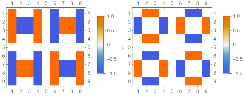
Figure 3: Solutions for $n=9$. The colourbar shows that the blue regions are $-1$, orange ones are $1$, and the rest zeroes. Notive how the $n=4$ solutions are neatly extended to form this basis.

For $6$ divides $n+1$, check that the solutions for the Moore neighbourhood also work for the Neumann neighbourhood and can be similarly extended from the $n=5$ case.

5.3 An interesting problem on harmonic functions

A discrete harmonic function [10] on a graph $G=(\mathcal{V},\mathcal{E})$ is defined as follows:

Definition 21.

A function $f:\mathcal{V}\to\mathbb{R}$ is harmonic at a node/vertex $x\in\mathcal{V}$ if it satisfies the following relation

$$f(x)=\frac{\sum_{\{x,y\}\in\mathcal{E}}f(y)}{deg(x)}$$

where $deg(x)$ is the degree of the vertex $x$.

Consider a toroidal chessboard with the Neumann neighbourhood condition i.e., two squares are neighbours iff they share a common edge. To define the associated graph $G$, we identify the squares with vertices and draw an edge between every neighbour or the torus. This creates a graph where every vertex has degree $4$.

Since every vertex is a representation of a cell on the toroidal board, we can denote a pair of coordinates $(p,q)$ to represent it, where $1\leq p\leq m,\;1\leq q\leq n$. It is easy to then find an appropriate transformation $T^{\circ+}_{m,n}$ whose kernel contains solutions of the modified neighbour sum equation

$$f(p,q+1)+f(p,q-1)+f(p+1,q)+f(p-1,q)=4f(p,q)$$

where if $(p,q)$ represents vertex $x$, then the tuples $(p\pm 1,q)$, $(p,q\pm 1)$ represents its Neumann neighbours. Note that this is not a neighbour sum problem, rather the mean tuple is one-fourth of the neighbour sum. Call this a Neumann-neighbour-average property of the vertex $x=(p,q)$.

Proposition 22.

The set of all $m\times n$ toroidal chessboards with the Neumann-neighbour-average property is precisely $ker(T^{\circ+}_{m,n})$, where

$$T^{\circ+}_{m,n}=B^{\circ}_{m}\oplus B^{\circ}_{n}-6\mathbb{I}_{m,n}$$

Proof.

The proof is along the same lines as that of Proposition 16. Here the matrices $B^{\circ}_{m},\;B^{\circ}_{n}$ correspond to adjacency matrices of circular graphs with self-loops. Further, in the final transformation $T^{\circ+}_{m,n}$, we require the diagonal elements to be $(-4)$ keeping all other elements constant, so we subtract $6\mathbb{I}_{m,n}$.         ∎

Proposition 23.

The space $\ker(T_{m,n}^{\circ+})$ is non-trivial if and only if there exist $p,q\in\mathbb{N}$ such that $1\leq p\leq m$, $1\leq q\leq n$ and

$$\cos\left(\frac{2p\pi}{m}\right)+\cos\left(\frac{2q\pi}{n}\right)=2$$

This eigenvalue equation has the trivial solution $\cos\left(\frac{2p\pi}{m}\right)=\cos\left(\frac{2q\pi}{n}\right)=1$, which gives $p=m,\;q=n$. So, the kernel is one-dimensional with the corresponding eigenvalues of $B^{\circ}_{m}$ and $B^{\circ}_{n}$ are both $3$.

Fact 24.

The eigenvectors of $A\oplus B$ are $\{x_{i}\otimes y_{j}\}$ where $\{x_{i}\}$ are the eigenvectors of $A$ and $\{y_{j}\}$ are the eigenvectors of $B$.

Note that eigenvectors of $B_{m}^{\circ}$ over $\mathbb{Z}^{m}$ for eigenvalue $=3$ are of the form $c\mathbbm{1}_{m}$, where $c\in\mathbb{Z}\backslash\{0\}$ is a constant. Then the corresponding unique solution (in vectorised format) is $c^{\prime}\mathbbm{1}_{m}\otimes\mathbbm{1}_{n}=c^{\prime}\mathbbm{1}_{mn},\;\;c^{\prime}\in\mathbb{Z}\backslash\{0\}$, which is just a constant.

This gives a neat result -

Theorem 25.

Discrete harmonic functions on a toroidal graph are constant functions.

Remark. If the same problem is specified on a finite square lattice, we could imagine the presence of a phantom boundary such that the mean-value property as defined is consistent. As the harmonic function takes the value zero on the boundary, by the maximum modulus principle for discrete harmonic functions[10], the only value it can take in the interior is identically zero. This can be shown with our linear algebra machinery, and is a nice connection between the two ideas.

6 Board extends to Infinity

At this juncture, it seems very natural to ask the same question for infinite chessboards. However, since an infinite board has fewer restrictions, it is much easier to answer this question.

A semi-infinite chessboard is one where the board is infinite in only one direction along the x and y axes. In that case, every square on the board can be expressed as a tuple $(i,j),\;i,j\in\mathbb{N}$. We do this numbering akin to that of rows and columns from the cell $(1,1)$ with only three neighbours sharing a common vertex or edge.

An infinite chessboard, which is infinite in both directions along the x and y axes is numbered as follows. Take a row and column and call them the 0-th row and column. Columns left of the 0-th column (resp. rows above the 0-th row) will be numbered by the negative integers while those right of (resp. below) would be numbered by the positive integers. The element at the intersection of the $i$-th row and $j$-th column is represented by the tuple $(i,j)$.

6.1 Semi-infinite chessboard

For a semi-infinite board, denote the value at any cell enumerated by $(i,j)$ as $x_{ij}$.

We can take any two sequences $\{a_{i}\}_{i=1}^{\infty}$ and $\{b_{i}\}_{i=1}^{\infty}$ (with $a_{1}=b_{1}$) to fill up the positions $\{(1,i)\}_{i=1}^{\infty}$ and $\{(i,1)\}_{i=1}^{\infty}$ respectively (enumeration begins from top left). Notice that the values at $(1,1),(1,2)$ and $(2,1)$ fixes $(2,2)$, call this value $x_{22}$.

$x_{22}$ along with the other given values fixes $x_{23}$ and $x_{32}$, and it is easy to check that done recursively, this fixes row 2 and column 2.

Note that in the first scenario, we could have used a phantom boundary beyond the first row and column to show that the existence of two adjacent filled rows and columns fixes the third row and column for semi-infinitely long axes. Recursively fixing elements, we can generate the solution. We are using a matrix notation just for clarity (this is not a matrix!).

$$\symking_{\mathbb{N}}=\begin{pmatrix}2&3&5&7&11&13&.&.&.\\ 3&-4&-3&2&-8&-3&.&.&.\\ 5&-3&-16&3&3&-42&.&.&.\\ 8&1&3&-15&37&29&.&.&.\\ 13&-8&-1&42&-86&99&.&.&.\\ 21&-7&-46&29&121&-428&.&.&.\\ .&.&.&.&.&.&.&.\\ .&.&.&.&.&.&.&.\\ .&.&.&.&.&.&.&.\\ \end{pmatrix}$$

6.2 Infinite chessboard

For an infinite board, it is again a matter of choosing the sequences $\{a_{i}\}_{i\in\mathbb{Z}\setminus\{0\}}$, $\{b_{i}\}_{i\in\mathbb{Z}\setminus\{0\}}$, $\{c_{i}\}_{i\in\mathbb{Z}\setminus\{0\}}$, and $\{d_{i}\}_{i\in\mathbb{Z}\setminus\{0\}}$ satisfying

$$a_{1}=b_{1},\qquad a_{-1}=d_{1},\qquad c_{1}=b_{-1},\qquad c_{-1}=d_{-1}$$

and putting them along any two rows and columns as shown in the figure below.

$$\symking_{\mathbb{Z}}=\begin{pmatrix}.&.&.&.&\astrosun&\astrosun&.&.&.&.\\ .&.&.&.&\astrosun&\astrosun&.&.&.&.\\ .&.&.&.&\astrosun&\astrosun&.&.&.&.\\ .&.&.&.&\astrosun&\astrosun&.&.&.&.\\ \astrosun&\astrosun&\astrosun&\astrosun&\astrosun&\astrosun&\astrosun&\astrosun&\astrosun&\astrosun\\ \astrosun&\astrosun&\astrosun&\astrosun&\astrosun&\astrosun&\astrosun&\astrosun&\astrosun&\astrosun\\ .&.&.&.&\astrosun&\astrosun&.&.&.&.\\ .&.&.&.&\astrosun&\astrosun&.&.&.&.\\ .&.&.&.&\astrosun&\astrosun&.&.&.&.\\ .&.&.&.&\astrosun&\astrosun&.&.&.&.\\ \end{pmatrix}$$

If the entries marked with $\astrosun$ are filled up with any sequences, they would divide the infinite board into four disjoint semi-infinite boards (disjoint since an any entry in each of the four quadrants would only depend upon the already filled numbers and not entries in any other quadrant). Further, each semi-infinite board contains a unique solution if two adjacent rows and columns are specified, which is the case here. Notice that the entries marked with $\astrosun$ can be first filled up by any numbers without already violating the neighbour-sum property.

7 Wrapping up

So, a simple problem inspired from a Math Olympiad paper has brought us a long way.

We first formulated a linear algebraic problem to tackle the problem, which led us to an eigenvalue equation. The key to solving that was rooted in certain tools of algebraic number theory and cyclotomic fields. This gave us a very powerful result to not only find explicit solutions for square boards, but also on rectangular and toroidal boards.

Changing the neighbourhood structure from Moore to von-Neumann also introduced some new interesting conditions for existence of solutions, and helped us explore a very interesting connection with discrete harmonic functions on graphs. Finally, we discussed in brief the simpler cases of semi-infinite and infinite boards (under Moore neighbourhood) - which makes for a very comprehensive take on the problem in two dimensions.

The next two sections would contain some rigorous mathematical insight into solving the relevant eigenvalue equations on higher dimensional grids (or lattice graphs), such as hypercubes. While there are a lot of different non-intuitive solutions that pop up in higher dimensions, we have tried to look at some easy to prove conditions that are generally true. The prospect of future work on those analogues is immense.

8 A brief Digression - some more Algebra

We wanted to get the integer $2$ as products of algebraic integers of the form

$$1+2\cos\left(\frac{2\pi p}{2(n+1)}\right)=1+\zeta_{m}^{a}+\zeta_{m}^{-a}=:\lambda_{a,m}$$

where $\frac{a}{m}$ is the reduced form of $\frac{p}{2(n+1)}$ . Naturally, we hoped that if one of these algebraic integers involving primitive $m$-th root of unity appeared in the product, all of its conjugates would too. This is true in two-dimensions, but a counter-example in three dimensions is as follows:

$$\left(1+2\cos\left(\frac{2\pi}{24}\right)\right)\left(1+2\cos\left(\frac{22\pi}{24}\right)\right)\left(1+2\cos\left(\frac{20\pi}{24}\right)\right)=2.$$

So, to get a sufficient condition for the existence of a solution we calculated the product of the conjugates i.e. the usual field norm [15] of $\lambda_{a,m}$ say $g(m)$, which would be an integer. If the product of some of these norms equals 2 and the total number of terms counting conjugates equals $d$, we get a solution.

Motivated by this, let us formally define

$$g(m):=\displaystyle\prod_{\begin{array}[]{c}1\leq a<\frac{m}{2}\\ \gcd(a,m)=1\end{array}}\left(1+2\cos\left(\frac{2\pi a}{m}\right)\right).$$

Observe that if we can write $2$ as the product of $g(m_{i})$’s where each $m_{i}\mid 2(n+1)$ and the “total length” of the product is $d$, we will have a solution in $d$ dimensions,

$$\prod_{i=1}^{d}\left(1+2\cos\left(\frac{p_{i}}{n+1}\right)\right)=2.$$

Here, by the length of $g(m_{i})$, we mean number of terms appearing in the product, i.e. $\frac{\phi(m_{i})}{2}$, and by total length we mean $\displaystyle\sum_{m_{i}}\frac{\phi(m_{i})}{2}$. As we’ll see in Theorem 28, $3\mid(n+1)$ is a necessary condition, if $2\mid(n+1)\implies 4\mid 2(n+1)$, we can choose $m_{1}=6$ and $m_{2}=\cdots=m_{d}=4$. This gives us a solution. To generalize the idea and get a better sufficient condition, we calculate $g(m)$ for different primes.

Theorem 26.

$$g(m)=\psi_{m}(-1)(-1)^{\frac{\phi(m)}{2}}=\Phi_{m}(\zeta_{3})(\zeta_{3})^{\frac{-\phi(m)}{2}}(-1)^{\frac{\phi(m)}{2}}$$

where $\Psi_{m}$ is the minimal polynomial of $2\cos\left(\frac{2\pi}{m}\right)$ [14, 17]and $\Phi_{m}$ is the $m$-th cyclotomic polynomial ([12] pg. 308) and $\zeta_{3}$ primitive 3rd root of unity.

Proof.

$$\Psi_{m}(x)=\displaystyle\prod_{\begin{array}[]{c}1\leq a<\frac{m}{2}\\ \gcd(a,m)=1\end{array}}\left(x-2\cos\left(\frac{2\pi a}{m}\right)\right)$$

Putting $x=-1$, we get the first equality. One can easily check that $\Psi_{n}\left(z+z^{-1}\right)=z^{-\frac{\phi(n)}{2}}\Phi_{n}(z)$. Putting $z=\zeta_{3}$, we get the second equality.         ∎

Now using this we can explicitly calculate $g(m)$ for any $m\in\mathbb{N},m>3$. We’ll show some of the relevant calculations here.

Theorem 27.

Let $p>3$ be a prime. Then,

$$g(p)=\left(\frac{3}{p}\right)=\begin{cases}1&\text{ if }p\equiv\pm 1\pmod{12}\\ -1&\text{ if }p\equiv\pm 5\pmod{12}\end{cases}$$

where $\left(\frac{{\color[rgb]{1,1,1}\cdot}}{{\color[rgb]{1,1,1}\cdot}}\right)$ is the Legendre symbol. Moreover, $g(2p)=1$ if $p\equiv 5\pmod{12}$.

Proof.

$\Phi_{p}(x)=1+x+\cdots+x^{p-1}$ and $\Phi_{2p}(x)=1-x+\cdots+x^{p-1}$.
$(-1)^{\frac{p-1}{2}}=\left\{\begin{array}[]{cc}1&\text{ if }p\equiv 1\pmod{4}\\ -1&\text{ if }p\equiv-1\pmod{4}\end{array}\right.$. ${\zeta_{3}}^{-(\frac{p-1}{2})}\Phi_{p}(\zeta_{3})=\left\{\begin{array}[]{cc}1&\text{ if }p\equiv 1\pmod{3}\\ -1&\text{ if }p\equiv-1\pmod{3}\end{array}\right.$.
Also, $\phi(p)=\phi(2p)$ for any odd prime and ${\zeta_{3}}^{-(\frac{p-1}{2})}\Phi_{2p}(\zeta_{3})=1$ if $p\equiv-1\pmod{3}$. This along with Theorem  26 gives us the proof.         ∎

9 Higher Dimensions and other generalisations

Using the tools developed in the previous sections, we will look at some nice results for higher dimensional analogues of the neighbour sum problem, such as on hypercubes. This is a natural extension of all our work til now, yet the conditions for existence or explicit solutions might be completely different from what we have observed. The problem can also be extended to arbitrary graphs or lattice-subsets in $Z^{d}$, but the problem becomes too complicated to even get a flavour of the kinds of solutions expected. Different tools might be needed to tackle them.

For example, start by considering the same problem on a $d$-dimensional hypercube. The analogue of the equation in Proposition 6 for this case is

$$\prod_{i=1}^{d}\left(1+2\cos\left(\frac{p_{i}}{n+1}\right)\right)=2$$

which is equivalent to trying to find the number of solutions of the equation

$$\sum_{i=1}^{d}v(\alpha_{i}+1+\alpha_{i}^{-1})=1$$

which now has a lot more combinations than was possible in the $d=2$ case. A criterion for existence of solutions is no longer as straightforward as on rectangles or squares. However, a necessary condition for existence is easy to figure out.

Theorem 28.

If an $n^{d}$ board satisfies the neighbour sum problem, then $3|(n+1)$.

Proof.

As already established, if $n^{d}$ board satisfies the problem, then the equation

$$\sum_{i=1}^{d}v(\alpha_{i}+1+\alpha_{i}^{-1})=1$$

has a solution.

But, this means that there is an $k$ such that $v(\alpha_{i}+1+\alpha_{i}^{-1})>0$, hence completing the proof.         ∎

Theorem 29.

If $6\mid(n+1)$ or $15\mid(n+1)$, there are solutions of

$$\prod_{i=1}^{d=3}\left(1+2\cos\left(\frac{p_{i}}{n+1}\right)\right)=2$$

.

Proof.

Let $6\mid n+1$, which gives $n+1=6k$ for some $k\in\mathbb{N}$. $p_{1}=2k\pi$, $p_{2}=p_{3}=3k\pi$ solves the eigenvalue equation.
Let $n+1=15k$. Then $p_{1}=5k\pi$, $p_{2}=3k\pi$, $p_{3}=9k\pi$ is a solution.         ∎

Numerical considerations urge us to make the following conjecture, which if true, should not be very difficult to prove for someone with the necessary expertise in Galois Theory:-
Conjecture. The converse of the Theorem  29 is true.

It is also not very difficult to arrive at a not-so-interesting sufficient condition for the problem for $n^{d}$ board. We have discussed the required language in Section 8.

By using Theorem  27, we give the sufficient condition for the existence of solutions.

Theorem 30.

Let $n+1=3^{a_{0}}p_{1}^{a_{1}}\cdots p_{r}^{a_{r}}q_{1}^{b_{1}}\cdots q_{s}^{b_{s}}$ where $q_{i}\equiv 7\pmod{12}$ and $p_{i}\not\equiv 7\pmod{12}$.

1. If any $p_{i}=2$ a solution of the form $g(6)g(4)\cdots g(4)=2$ exists.

2. If all $p_{i}$’s are odd primes, then if there are integers $x_{1},\cdots,x_{r},y_{1},\cdots,y_{s}\geq 0$ such that

   $$x_{1}\left(\frac{p_{1}-1}{2}\right)+\cdots+x_{r}\left(\frac{p_{r}-1}{2}\right)+2y_{1}\left(\frac{q_{1}-1}{2}\right)+\cdots+2y_{s}\left(\frac{q_{s}-1}{2}\right)=d-1$$

   a solution exists and is given by by

   $$g(6)g(p^{\prime}_{1})^{x_{1}}\cdots g(p^{\prime}_{r})^{x_{r}}g(q_{1})^{2y_{1}}\cdots g(q_{s})^{2y_{s}}=2$$

   Here $p^{\prime}_{i}=2p_{i}$ if $p_{i}\equiv 5\pmod{12}$ and $p^{\prime}_{i}=p_{i}$ otherwise.

Proof.

It is enough to explicitly compute the form of the solutions.         ∎

We have also previously established that for $d=2$, whenever we have a solution, the solution space is two dimensional. This motivates us to ask the question for higher dimensional analogues of the problem. For this question, we do not have any useful results to present. We give the sequence $\{a_{n}^{d}\}_{n\geq 2}$ of number for solutions of $n^{d}$ boards obtained numerically.

d=3 :
0, 0, 0, 3, 0, 0, 0, 0, 0, 15, 0, 0, 6, 0, 0, 3, 0, 0, 0, 0, 0, 15, 0, 0, 0, 0, 0, 9, 0, 0, 0, 0, 0, 15, 0, 0, 0, 0, 0, 3, 0, 0, 6, 0, 0, 15, $\ldots$

d=4 :
0, 0, 0, 4, 0, 0, 0, 0, 0, 88, 0, 0, 24, 0, 0, 4, 0, 0, 0, 0, 0, 136, 0, 0, 0, 0, 0, 220, 0, 0, 0, 0, 0, 88, 0, 0, 48, 0, 0, 52, 0, 0, 24, 0, 0, 136, $\ldots$

d=5 :
0, 0, 0, 5, 0, 0, 0, 0, 0, 335, 0, 0, 480, 0, 0, 485, 0, 0, 540, 0, 0, 1295, 0, 0, 0, 0, 0, 1865, 0, 0, 0, 0, 0, 815, 0, 0, 0, 0, 0, 1385, 0, 0, 480, 0, 0, 2255, $\ldots$

One might be interested to find patterns in these sequences - a task left to the inquisitive reader.

We conclude our paper with a small remark on extending the neighbour-sum property to custom graphs. In our paper, we defined a transformation whose kernel contains the relevant solutions. The key step was to decompose the graph (subset of $\mathbb{Z}^{2}$) into Cartesian products of line-graphs (or cycle graphs), which translates neatly over to the adjacency matrix representations through Kronecker prodcuts and sums. Similar decompositions for custom graphs can help in reducing the difficulty of the problem and introduce several interesting ideas. One might need a thorough understanding of spectral graph theory and linear algebra to tackle such general problems.

10 Acknowledgments

We would like to acknowledge the contribution of Prof. Dr. David E. Speyer for his contributions to formulating the proof of our main existence theorem on square boards as well as ideas regarding its generalisation. We would also like to thank our batchmates in CS for helping out with generation of numerical solutions and relevant sequences. We are indebted to their help in succesfully completing this paper early.

References

- [1] Daniel Berend, Ephraim Korach, and Shira Zucker. Two-anticoloring of planar and related graphs. Discrete Mathematics & Theoretical Computer Science, (Proceedings), 2005.
- [2] Norman Biggs. Algebraic graph theory. Number 67. Cambridge university press, 1993.
- [3] Gerard J Chang. Algorithmic aspects of domination in graphs. Handbook of Combinatorial Optimization: Volume1–3, pages 1811–1877, 1998.
- [4] John Conway and A Jones. Trigonometric diophantine equations (on vanishing sums of roots of unity). Acta arithmetica, 30:229–240, 1976.
- [5] Philip J Davis. Circulant matrices wiley. New york, 1979.
- [6] Phoebus J. Dhrymes. Matrix Vectorization, pages 117–145. Springer New York, New York, NY, 2000.
- [7] David Steven Dummit and Richard M Foote. Abstract algebra, volume 3. Wiley Hoboken, 2004.
- [8] Gena Hahn and Gert Sabidussi. Graph symmetry: algebraic methods and applications, volume 497. Springer Science & Business Media, 2013.
- [9] Allen Hatcher. Algebraic topology. 2005.
- [10] Hans A Heilbronn. On discrete harmonic functions. In Mathematical Proceedings of the Cambridge Philosophical Society, volume 45, pages 194–206. Cambridge University Press, 1949.
- [11] Harold V Henderson, Friedrich Pukelsheim, and Shayle R Searle. On the history of the kronecker product. Linear and Multilinear Algebra, 14(2):113–120, 1983.
- [12] I Martin Isaacs. Algebra: a graduate course, volume 100. American Mathematical Soc., 2009.
- [13] Devadatta Kulkarni, Darrell Schmidt, and Sze-Kai Tsui. Eigenvalues of tridiagonal pseudo-toeplitz matrices. Linear Algebra and its Applications, 297:63–80, 1999.
- [14] Derik H Lehmer. A note on trigonometric algebraic numbers. Amer. Math. Monthly, 40(3):165–166, 1933.
- [15] Joseph J Rotman. Advanced modern algebra, volume 114. American Mathematical Soc., 2010.
- [16] John Von Neumann, Arthur W Burks, et al. Theory of self-reproducing automata. IEEE Transactions on Neural Networks, 5(1):3–14, 1966.
- [17] William Watkins and Joel Zeitlin. The minimal polynomial of ). The American Mathematical Monthly, 100(5):471–474, 1993.