First Adiabatic Invariant and the Brightness Temperature of Relativistic Jets

DOI: 10.1134/S1063773723030015
Keywords: active galaxies, jets.

Introduction

Relativistic jets from active galactic nuclei (AGNs) are apparent manifestations of their activity at an early stage of evolution (Begelman et al. 1984; Urry and Padovani 1995; Davis and Tchekhovskoy 2020; Komissarov and Porth 2021). Their hydrodynamic velocities correspond to Lorentz factors $\Gamma\sim$ 10. In the galaxy M87 this motion is observed directly, while the Lorentz factor is $\Gamma\approx 6$ (Junor and Biretta 1995). In many cases, the outflowing plasma retains relativistic velocities at enormous distances from the nucleus before decelerating noticeably when interacting with the intergalactic medium. There is no doubt that the observed radio emission of the jet is associated with the synchrotron radiation of relativistic electrons. This is suggested both by the power-law spectrum of the observed emission and by its characteristic low-frequency cutoff easily explainable by synchrotron self-absorption (Lyutikov et al. 2003, 2005; Porth et al. 2011; Sokolovsky et al. 2011).

At present, owing to the development of very long baseline interferometry (VLBI), it is possible to trace the properties of the radio emission up to the innermost (of the order of hundreds of gravitational radii) jet regions (Kovalev et al. 2005). In particularly, it has been shown recently that in many cases the jet shape changes from parabolic to conical (Asada and Nakamura 2012; Kovalev et al. 2020; Park et al. 2021; Boccardi et al. 2021), so that this phenomenon can be said to be universal for relativistic jets. However, despite the large volume of accumulated information, many issues still await their resolution. In particular, this concerns the recently detected break in the dependence of the brightness temperature $T_{\rm br}$ on the distance to the ”central engine” $z$ (Kadler et al. 2004; Baczko et al. 2019; Burd et al. 2022) that occurs in many cases at distances $\sim$ 1 pc, i.e., exactly in the region of the transition from parabolic to conical shape. This break is observed already in dozens of objects, with the exponents $a$ in the power law $T_{\rm br}\propto z^{-a}$ being confined in a wide range,

$$a_{1} = 3.0\pm 1.0,$$ (1)

$$a_{2} = 2.7\pm 1.0,$$ (2)

where $a_{1}$ and $a_{2}$ correspond to small and large distances from the central engine, respectively. Such a wide spread of parameters, when close mean values contain little information, implies that in some cases $a_{1}>a_{2}$ (upward break), while in other cases $a_{1}<a_{2}$ (downward break). At the same time, no difference in the exponents a for quasars and BL Lac objects is observed.

One of the reasons restraining the construction of a consistent theory of radio emission from jets was that the energy of radiating particles should be much greater than the energy of hydrodynamic motion. Therefore, for many years it had been impossible to directly connect the questions related to the observed radio emission with the magnetohydrodynamic (MHD) theory of jets that had already been developed for several decades (Heyvaerts and Norman 1989; Pelletier and Pudritz 1992; Beskin 2006; Tchekhovskoy et al. 2008; McKinney et al. 2012), since the MHD theory of jets told us nothing about the energetics of radiating particles. Since so far there had been no consensus on the formation of the spectrum of radiating particles (see, e.g., Marscher and Gear 1985; Istomin and Pariev 1996; Pariev et al. 2003), the uncertainty arising in this link did not allow the evolution of the emission parameters along the jet axis to be investigated self-consistently.

As a matter of fact, only the adiabatic model of Marscher (1980) is currently a sufficiently well-developed model that allows the dependence of the spectrum of radiating particles on the distance to the central engine $z$ to be analyzed. Indeed, using the relativistic equation of state $PV^{4/3}=$ const for a conical jet, when the size of the emitting regions $R\propto z$, we immediately obtain $\gamma\propto R^{-2/3}$ for the average Lorentz factor. These approximations were generalized to the situation of accelerating jets already in Lobanov and Zensus (1999). Subsequently, based on the results presented above, Lobanov et al. (2000) derived a dependence of the brightness temperature on the transverse size of the jet in the form $T_{\rm br}\sim R^{-\xi}$ ($\xi\approx 2$), where $R$ is the transverse size of the jet. For example, such a dependence was applied for the observed changes in brightness temperature in Goméz et al. (2016) and Nair et al. (2019).

However, it is not obvious that such a simple hydrodynamic model will be valid for a strongly magnetized flow as well. In any case, for radiating particles their mean free path $l_{\gamma}$ (Berestetskii et al. 1989),

$$l_{\gamma}\sim\frac{\gamma^{2}}{r_{\rm e}^{2}n}\sim 10^{8}\,R_{\rm L}\left(\frac{\lambda}{10^{12}}\right)^{-1}\left(\frac{\gamma}{10^{3}}\right)^{2}\left(\frac{B_{\rm p}}{10\rm{G}}\right)^{-1},$$ (3)

turns out to be greater than the characteristic size of the system $L$. Here, $\lambda$ is a convenient dimensionless coefficient (production multiplicity) that parameterizes the particle number density

$$n_{\rm e}=\lambda n_{\rm GJ},$$ (4)

where $n_{\rm GJ}=\Omega_{\rm F}B_{\rm p}/(2\pi\,c\,e)$ is so-called Goldreich-Julian number density, i.e., the minimum particle number density needed for the approximation of ideal magnetohydrodynamics to hold, and $\Omega_{\rm F}\approx\Omega_{\rm H}/2$, where $\Omega_{\rm H}$ is the black hole rotation rate. Finally, $R_{\rm L}=c/\Omega_{\rm F}$ is the radius of the light cylinder, which exceeds the black hole radius approximately by a factor of 10 (Davis and Tchekhovskoy 2021; Komissarov and Porth 2021). We used a poloidal magnetic field $B_{\rm p}=10^{2}$ G typical for the scale of the light cylinder. As regards $\lambda$, below we set $\lambda\sim 10^{12}$. Such a large value follows both from numerical simulations of particle production in the magnetospheres of black holes (Mościbrodzka et al. 2011) and from observations (Nokhrina et al. 2015).

Of course, the condition $l_{\gamma}\gg L$ is insufficient for the relation $PV^{4/3}=$ const to break down; this requires that the distribution function be isotropized sufficiently slowly, while this process depends on the level of outflowing plasma turbulence, about which there is currently no reliable information. Therefore, below we consider a two-component model consisting of a hydrodynamic flow with a small spread of particles in energies (for which the isotropization condition is fulfilled) and a high-energy tail of weakly interacting particles with which the observed synchrotron radiation is associated. To explain the observed radiation (including the optical and X-ray one), it is commonly assumed that the power-law spectrum can extend to energies at least of the order of several TeV. The number density of radiating particles should be noticeably lower than the background plasma number density.

It is natural to assume that the first adiabatic invariant $I_{\perp}=p_{\perp}^{2}/B$ will be conserved for radiating particles. In this case, it will also be possible to relate their energetics to the jet parameters, which, as has already been noted, are satisfactorily modeled within present-day MHD models. As a result, a unique opportunity to obtain direct information about the evolution of the emitting plasma properties along the jet axis appears. In particular, it becomes possible to check whether an additional particle acceleration within the jet is necessary to explain the intensity of the observed radiation.

In this paper, based on our analysis of the motion of charged particles in conical and parabolic relativistic jets, we investigate the change in brightness temperature along the jet axis. We show that in this case the observed break in the dependence of the brightness temperature on the distance to the central engine can be explained. Good agreement with observations is achieved without any additional particle acceleration within the jet itself.

In the first part we discuss two models of relativistic jets that describe quite adequately the internal structure of relativistic jets from AGNs. The second part is devoted to analyzing the conservation of the first adiabatic invariant in the crossed electric and magnetic fields of relativistic jets. We show that the first adiabatic invariant is conserved with a great accuracy. Finally, in the third part we analyze the pattern of change in brightness temperature along the jet axis through a different dependence of the behavior of the radiating particle spectrum due to the conservation of the first adiabatic invariant. We show that this effect can serve as a basis for explaining the observational data.

Two models of relativistic jets

As has already been noted above, the observations themselves suggest that conical and parabolic flows may be chosen as a fairly good geometrical model of relativistic jets. Therefore, as a basis, below we consider two simple analytical models of forcefree relativistic jets — the conical (to be more precise, quasi-spherical) solution of Michel (1973) and the parabolic solution of Blandford (1976). Here an important help to us is the fact that, according to numerical simulations (see, e.g., McKinney et al. 2012), a substantial region near the jet axis does have a regular magnetic field.

The electromagnetic fields of Michel’s conical force-free flow in spherical coordinates $r$, $\theta$, $\varphi$ are

$$B_{r} = B_{\rm L}\frac{R_{\rm L}^{2}}{r^{2}},$$ (5)

$$B_{\varphi} = -B_{\rm L}\frac{R_{\rm L}}{r}\sin\theta,$$ (6)

$$E_{\theta} = -(1-\varepsilon)B_{\rm L}\frac{R_{\rm L}}{r}\sin\theta,$$ (7)

where again $R_{\rm L}$ is the radius of the light cylinder and $B_{\rm L}$ is the magnetic field at $r=R_{\rm L}$. We assume that this solution exists only in the narrow region $\theta<\theta_{\rm jet}\sim 0.1$ near the jet axis. In addition, the factor $\left(1-\varepsilon\right)$ was added to the expression for the electric field, where the constant $\varepsilon\ll 1$ allows one to simulate the absence of particle acceleration at great distances, when the entire electromagnetic energy flux has been transferred to the plasma flow. In other words, the small parameter $\varepsilon$ is responsible for the saturation of the particle energy (Lorentz factor).

Indeed, using the fundamental theoretical result that in an asymptotically distant region beyond the light cylinder the particle energy in the hydrodynamic component approaches the energy corresponding to drift motion (Tchekhovskoy et al. 2008; Beskin 2010; Bogovalov 2014)

$${\bf U}_{\rm dr}=c\frac{{\bf E}\times{\bf B}}{B^{2}},$$ (8)

and, therefore, the longitudinal velocity along the magnetic field may be neglected when determining the hydrodynamic velocity of the particles, for the hydrodynamic Lorentz factor we obtain

$$\Gamma=\frac{1}{\sqrt{1-v^{2}/c^{2}}}=\left(1-\frac{E^{2}}{B_{\varphi}^{2}+B_{\rm p}^{2}}\right)^{-1/2}\approx$$

$$\approx\left(1-\frac{1-2\varepsilon}{1+1/x^{2}}\right)^{-1/2}\approx\left(2\varepsilon+\frac{1}{x^{2}}\right)^{-1/2}.$$ (9)

Here, $x=r\sin\theta/R_{\rm L}$ is the dimensionless distance to the jet axis. As a result, at small distances from the central engine, i.e., at $x<(2\varepsilon)^{-1/2}$, we obtain

$$\Gamma\approx x,$$ (10)

i.e., the well-known asymptotic behavior for collimated magnetized jets. On the other hand, at great distances, i.e., at $x>(2\varepsilon)^{-1/2}$, we have $\Gamma\approx(2\varepsilon)^{-1/2}\approx$ const. This asymptotic solution simulates the saturation region, when the entire energy flux is concentrated in the hydrodynamic particle flow. Therefore, we can write

$$\varepsilon\approx\frac{1}{2\sigma_{\rm M}^{2}},$$ (11)

where $\sigma_{\rm M}$ is the so-called Michel (1969) magnetization parameter that has the meaning of a maximally possible Lorentz factor. According to Nokhrina et al. (2015), for most of the relativistic jets from AGNs $\sigma_{\rm M}=10$–$50$, consistent with the values determined from superluminal motions. Thus, the structure of the electromagnetic fields unambiguously determines all of the hydrodynamic flow characteristics needed for us below.

Another model is the force-free solution with a parabolic poloidal magnetic field found by Blandford (1976). In spherical coordinates $r$, $\theta$, $\varphi$ it can be written as (Beskin 2006)

$${\bf B}_{\rm p}=B_{\rm L}\frac{\nabla X\times{\bf e}_{\varphi}}{\sin\theta\sqrt{1+\Omega_{\rm F}(X)^{2}X^{2}/c^{2}}}\frac{R_{\rm L}}{r}\mbox{,}$$ (12)

where $R_{\rm L}=c/\Omega_{\rm F}(0)$ and

$$X=r(1-\cos\theta),$$ (13)

so $|\nabla X|=\sqrt{2-2\cos\theta}$. The condition $X(r,\theta)=$ const ($\theta\propto r^{-1/2}$) corresponds to a parabolic structure whereby all field lines pass through the equatorial plane (with the central part of the field lines crossing the black hole horizon). The radius of the light cylinder $R_{L}$ and the value of the function $\Omega_{F}$ at $X=0$ are related by the condition $R_{\rm L}=c/\Omega_{\rm F}(0)$. Accordingly, the electric and toroidal magnetic fields are

$${\bf E}=-\frac{B_{\rm L}(1-\varepsilon)}{\sqrt{1+\Omega_{\rm F}(X)^{2}X^{2}/c^{2}}}\,\times$$

$$\times\left(\frac{\Omega_{\rm F}(X)R_{\rm L}}{c}\right)\,\nabla X,$$ (14)

$$B_{\varphi}=-\frac{B_{\rm L}}{\sqrt{1+\Omega_{\rm F}(X)^{2}X^{2}/c^{2}}}\times$$

$$\times\frac{(2-2\cos\theta)}{\sin\theta}\,\left(\frac{\Omega_{\rm F}(X)R_{\rm L}}{c}\right).$$ (15)

Here, $\Omega_{\rm F}$, the so-called angular velocity of the magnetic field lines, must depend on $X$, since only those configurations for which $\Omega\left(X\right)X/c<1$ turn out to be possible (otherwise the central engine would rotate with a speed exceeding the speed of light); in all of the subsequent calculations we assumed that $\Omega\left(X\right)X/c=0.5$ at $X>0.5\,R_{\rm L}$. Here, by analogy with the previous model, the constant factor $\left(1-\varepsilon\right)$ was added to the electric field. It is easy to verify that for this configuration the asymptotic behavior $\Gamma=x$ (10) also holds in the region of a strongly magnetized flow and $\Gamma\approx$ const in the saturation region.

Conversation of the first adiabatic invariant

Before turning to our main problem, i.e., finding the brightness temperature of relativistic jets, let us discuss in detail the properties of the motion of individual particles in the electromagnetic fields defined above. First of all, it is necessary to check whether the first adiabatic invariant

$$I_{\perp}=\frac{(p_{\perp}^{\prime})^{2}}{h}.$$ (16)

is indeed be conserved during such a motion. Here,

$$h=\sqrt{B^{2}-E^{2}}$$ (17)

is the magnetic field in the hydrodynamic rest frame (the electric field is zero). Accordingly, $p_{\perp}^{\prime}$ is the transverse momentum also in the rest frame. The point is that in the standard formulation the motion of a particle is considered in a stationary magnetic field, i.e., in a specified inertial reference frame. In contrast, in our case the comoving reference frame (the reference frame in which the plasma is at rest) accelerates in inhomogeneous crossed electric and magnetic fields. Therefore, it is useful to check the conservation of the first adiabatic invariant in such a nontrivial case.

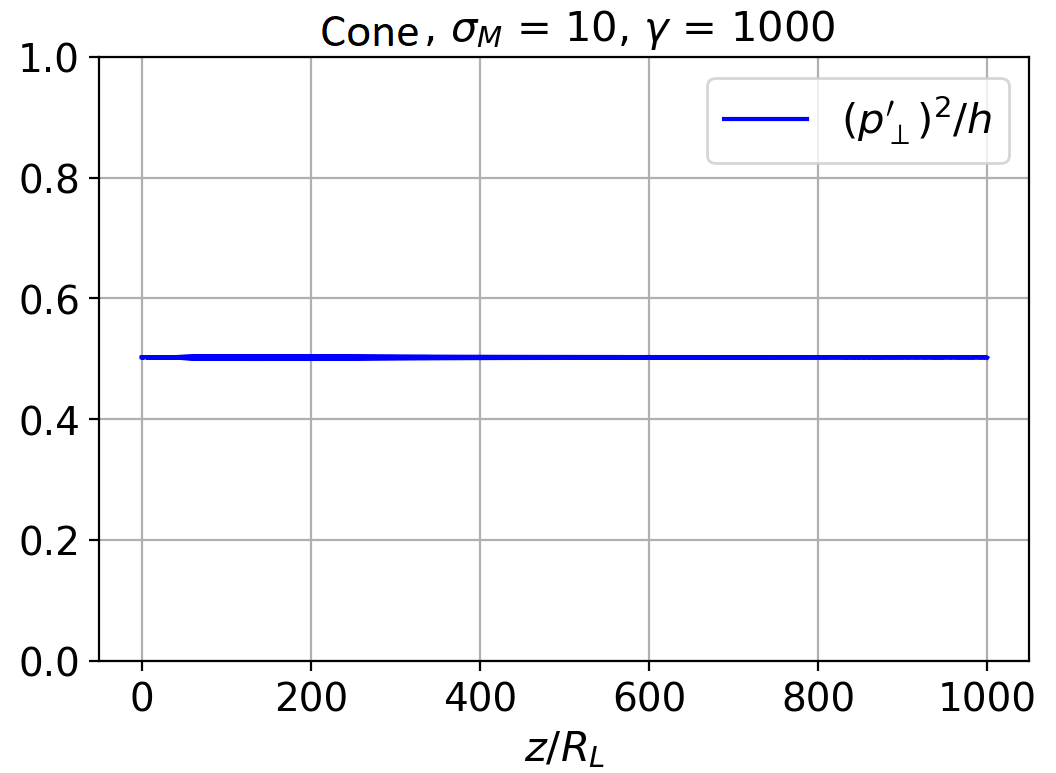
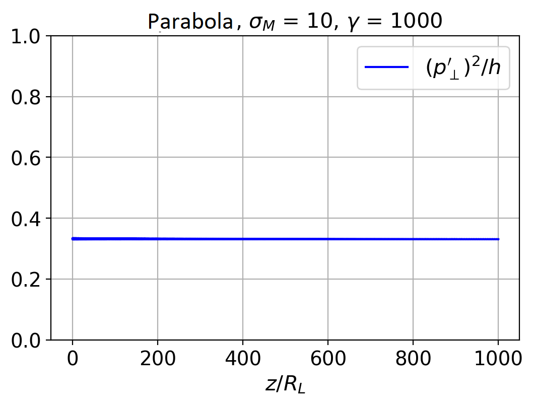
Figure 1: . Conservation of the first adiabatic invariant in the comoving reference frame (relative units) for conical and parabolic flows.

Figure 1 shows the results of our numerical integration of the motion of particles in the electromagnetic fields (5)–(7) and (14)–(15) for typical parameters of relativistic jets, $\sigma_{\rm M}=10$ and the Lorentz factor $\gamma=10^{3}$; the value of the small parameter $\varepsilon$ is determined from relation (11). As we see, the first adiabatic invariant $I_{\perp}$ (16) is indeed conserved with a good accuracy for both conical and parabolic geometries. Since for ultrarelativistic radiating particles $m_{\rm e}c\gamma^{\prime}\approx p_{\perp}^{\prime}$, we find that

$$\gamma^{\prime}=\frac{I_{\perp}^{1/2}}{m_{\rm e}c}\,h^{1/2}.$$ (18)

Here, it is also important to draw attention to the fact that the invariant $I_{\perp}$ does not change while the pattern of the dependence of $h$ on the distance $z$ to the central engine changes significantly. Indeed, it is easy to verify, using relation (9), that for a conical flow at small distances, i.e., at $x<1/\sqrt{2\varepsilon}$, the asymptotic behavior $h\propto z^{-2}$ is valid, while at great distances $x>1/\sqrt{2\varepsilon}$ the asymptotic behavior $h\propto z^{-1}$ is valid. Accordingly, for a parabolic flow at small distances, i.e., at $x<1/\sqrt{2\varepsilon}$, we have $h\propto z^{-1}$ and $h\propto z^{-1/2}$ at great distances $x>1/\sqrt{2\varepsilon}$. As we show, it is the presence of such a break that allows us to explain the pattern of change in the dependence of the brightness temperature on the distance $z$ to the central engine.

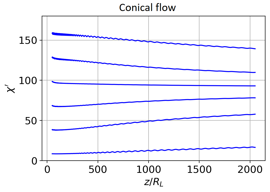
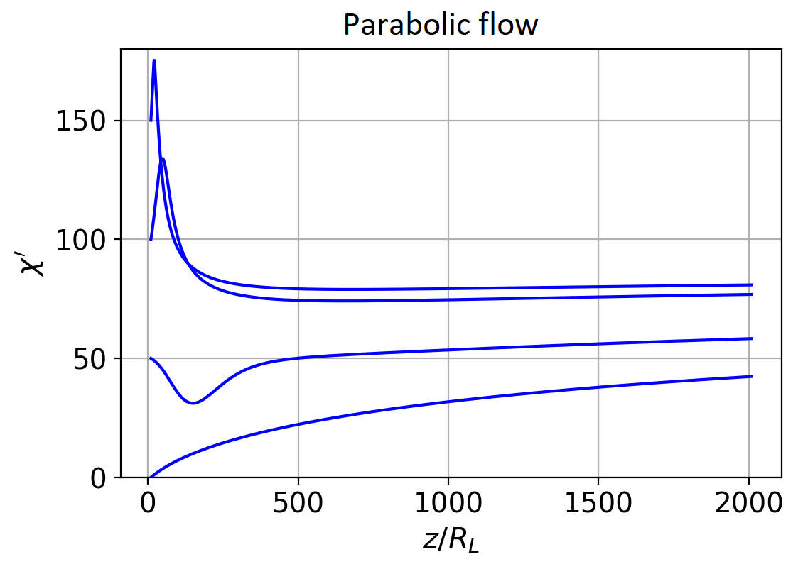
Figure 2: Pitch angle of an individual particle $\chi^{\prime}$ in the comoving reference frame versus distance $z$ to the central engine.

Finally, note yet another important circumstance that we need below. As shown in Fig. 2, in the comoving reference frame the pitch angle of an individual particle $\chi^{\prime}$ does not decrease with decreasing magnetic field (i.e., with increasing distance $z$ to the central engine), as is sometimes the case in static, purely magnetic configurations, but, on the contrary, though slowly, tends to $90^{\circ}$. This once again confirms the previously noted result that in magnetized winds (and in the comoving reference frame) the longitudinal (parallel to the magnetic field) velocity component may be neglected compared to the drift velocity. It is clear that this effect takes place only beyond the light cylinder, where the role of the electric field becomes decisive. In contrast, within the light cylinder, as in the absence of an electric field, the conservation of the first adiabatic invariant leads to a decrease in the pitch angle $\chi^{\prime}$ . Such a decrease in $\chi^{\prime}$ is clearly seen in Fig. 2 for a parabolic field at the initial phase of the particle trajectories, as long as they are in the immediate vicinity of the light cylinder. As has already been noted, the various instabilities inherent in highly anisotropic distributions tend to reduce the degree of anisotropy. Therefore, the assumption about slow isotropizatrion is a necessary condition for the model being considered here. Only the fact that the pitch angles do not tend to $0^{\circ}$, when the synchrotron radiation power is substantially suppressed, will be important to us below.

Brightness temperature

Let us now look at how the change in the energy of radiating particles that inevitably arises as the jet expands due to the conservation of the first adiabatic invariant affects the change in brightness temperature $T_{\rm br}$ along the jet axis. Here we use the standard relations derived in Lyutikov et al. (2003, 2005). A significant difference lie only in the fact that we take into account both the jet expansion and the evolution of the spectrum of radiating particles. At the same time, we ignore the synchrotron losses in the high-energy part of the spectrum (see the Appendix).

Note at once that the possibility to restrict ourselves to the approximation of an optically thin plasma, in which neither the synchrotron self-absorption nor the Faraday rotation is taken into account, stems from the fact that the saturation region of interest to us here is sufficiently far from the central engine, where the plasma density and the magnetic fields are already not so great. As is well known, in the centimeter wavelength range there is noticeable self-absorption determined from the core shift (see, e.g., Nokhrina et al. 2015) at distances no greater than several hundred gravitational radii. Regarding the Faraday rotation, as is well known, even the rotation measures ${\rm RM}\sim 100$ rad m^-2 recorded in the innermost regions (Kravchenko et al. 2017; Gabuzda et al. 2017) do not lead to noticeable depolarization in the centimeter wavelength range.

Below we will present the corresponding calculations, while here we will begin our discussion with the expression for the number density of radiating particles in the comoving reference frame $n_{\gamma}^{\prime}$ with a power-law energy spectrum in the range $\gamma_{0}<\gamma^{\prime}<\gamma_{\rm max}$:

$${\rm d}n_{\gamma}^{\prime}=K_{\rm e}\,(\gamma^{\prime})^{-p}\,{\rm d}\gamma^{\prime}\,{\rm d}^{3}{r}^{\prime}\,{\rm d}\Omega.$$ (19)

Here, $p$ is the spectral index, ${\rm d}\Omega$ is an element of the solid angle, and $K_{\rm e}$ is the normalization constant. Note at once that in our model it is important that the lower limit integration plays a key role. As we show below, the lower limit can also correspond to nonrelativistic velocities ($\gamma_{0}=1$); our main conclusions will not change because of that.

Next, note that owing to the tendency for the pitch angle $\chi^{\prime}$ to increase, which is pointed out above, in this paper we will ignore the dependence of the distribution function (19) on the solid angle ${\rm d}\Omega$. This is because at small angles between the jet axis and the direction to the observer typical for quasars and owing to the nearly toroidal magnetic field in the main part of the jets, the synchrotron radiation beam of most radiating particles will be oriented toward the observer.

As a result, since, as has been shown above, the energy of all radiating particles when propagating along the expanding jet changes proportionally to $h$, the power-law shape of the spectrum is retained along the entire jet. On the other hand, if the normalization of the particle energy spectrum is chosen in the form $\int f(\gamma^{\prime}){\rm d}\gamma^{\prime}=1$, then in this case

$$K_{\rm e}=(p-1)n_{\gamma}^{\prime}({\bf r}^{\prime})\,\gamma_{0}^{p-1}({\bf r}^{\prime}).$$ (20)

Here, we assumed that $\gamma_{\rm max}^{\prime}\gg\gamma_{0}$ and $\gamma_{0}\gg 1$. Owing to the main relation $\gamma_{0}\propto h^{1/2}$ (18), the normalization factor $K_{\rm e}$ acquires a dependence on the invariant $h$. This allowance for the dependence of $K_{\rm e}$ on the coordinates in agreement with the conserved adiabatic invariant $I_{\perp}$,

$$K_{\rm e}\propto n_{\gamma}^{\prime}\,h^{(p-1)/2},$$ (21)

due to the dependence of the magnetic field in the comoving reference frame $h$ on distance $z$, that is the subject of our study. It is easy to verify that the dependence (21) will also hold if the lower boundary of the spectrum of radiating particles is close to $m_{\rm e}c^{2}$ ($\gamma_{0}=1$). In this case, the change in $K_{\rm e}$ is related to the change in the number of radiating particles with $\gamma^{\prime}>1$.

Using now the standard expression for the intensity $I_{\nu}$ (Lyutikov et al. 2005), we obtain

$${\rm d}I_{\nu}=2\pi\frac{(p+7/3)}{(p+1)}\,\kappa(\nu)\,\frac{{\rm d}S\,{\rm d}l}{D^{2}}\,\times$$

$$\times{\cal D}^{2+(p-1)/2}\,|h\sin{\hat{\chi}}|^{(p+1)/2}\,{\rm d}\nu.$$ (22)

Here, $\hat{\chi}$ is the angle between the magnetic field and the line of sight,

$$\kappa(\nu)=\frac{\sqrt{3}}{4}\Gamma\left(\frac{3p-1}{12}\right)\Gamma\left(\frac{3p+7}{12}\right)\,\times$$

$$\ \times\frac{e^{3}}{m_{\rm e}c^{2}}\,\left(\frac{3e}{2\pi m_{\rm e}c}\right)^{(p-1)/2}\nu^{-(p-1)/2}K_{\rm e},$$ (23)

$D$ is the distance to the source, and

$${\cal D}=\frac{1}{\Gamma(1-{\boldsymbol{\beta}}{\bf n})}$$ (24)

is the Doppler factor (${\boldsymbol{\beta}}={\bf v}/c$, where ${\bf v}$ is the hydrodynamic velocity and ${\bf n}$ is a unit vector in the observer’s direction). Next, the volume element (which must already correspond to the laboratory reference frame in this relation) is written as ${\rm d}^{3}r={{\rm d}S\,{\rm d}l}$, where ${\rm d}S$ is a surface element perpendicular to the line of sight and ${\rm d}l$ is a length element along the line of sight. Finally, since ${\rm d}S/D^{2}$ is an element of the solid angle, for the brightness temperature $T_{\rm br}=I_{\nu}c^{2}/(2k_{\rm B}\nu^{2})$ we ultimately obtain

$$T_{\rm br}=R(p)\frac{e^{3}}{m_{\rm e}k_{\rm B}}\,\left(\frac{e}{m_{\rm e}c}\right)^{(p-1)/2}\nu^{-(p+3)/2}\times$$

$$\times\int{\cal D}^{2+(p-1)/2}h^{(p+1)/2}n_{\gamma}({\bf r})\,\times$$

$$\times\gamma_{0}^{p-1}({\bf r})(\sin{\hat{\chi}})^{(p+1)/2}{\rm d}l,$$ (25)

where now $n_{\gamma}({\bf r})$ is the particle number density in the laboratory frame, $k_{\rm B}$ is the Boltzmann constant,

$$R(p)=\frac{3^{p/2}}{8(2\pi)^{(p-3)/2}}\frac{(p-1)(p+7/3)}{(p+1)}\times$$

$$\times\Gamma\left(\frac{3p-1}{12}\right)\Gamma\left(\frac{3p+7}{12}\right),$$ (26)

and the integral is taken along the line of sight.

Next, let us again express the number density of radiating particles $n_{\gamma}$ via the Goldreich-Julian number density $n_{\rm GJ}$ (2):

$$n_{\gamma}=\lambda_{\gamma}n_{\rm GJ},$$ (27)

where the constant $\lambda_{\gamma}$,

$$\lambda_{\gamma}\ll\lambda,$$ (28)

is the multiplicity of radiating particles, while at $\theta\ll 1$, when $z\approx r$,

$$n_{\rm GJ}=\frac{B_{\rm L}}{2\pi e}\frac{R_{\rm L}}{r^{2}}\cos\theta\approx 1.1\cdot 10^{-5}\,\mbox{cm}^{-3}\times$$

$$\times\left(\frac{h_{0}}{100\,\mbox{G}}\right)\left(\frac{R_{\rm L}}{10\,r_{\rm g}}\right)^{-1}\left(\frac{M_{\rm bh}}{10^{9}M_{\odot}}\right)^{-1}\left(\frac{z}{R_{\rm L}}\right)^{-2}$$ (29)

for electromagnetic fields with a conical shape of the magnetic surfaces (5)–(7) and

$$n_{\rm GJ}=\frac{B_{\rm L}}{\sqrt{5}\pi er}\approx 1.0\cdot 10^{-5}\,\mbox{cm}^{-3}\times$$

$$\times\left(\frac{h_{0}}{100\,\mbox{G}}\right)\left(\frac{R_{\rm L}}{10\,r_{\rm g}}\right)^{-1}\left(\frac{M_{\rm bh}}{10^{9}M_{\odot}}\right)^{-1}\left(\frac{z}{R_{\rm L}}\right)^{-1}$$ (30)

for electromagnetic fields with a parabolic shape of the magnetic surfaces (12), (14), and (15) at $X/R_{\rm L}<0.5$ and constant $\Omega_{\rm F}=c/R_{\rm L}$.

As a result, we obtain

$$T_{\rm br}=\lambda_{\gamma}\frac{m_{\rm e}c^{2}}{k_{\rm B}}\frac{R(p)}{2\pi}\left(\frac{eh_{0}}{m_{\rm e}c}\right)^{(p+3)/2}\nu^{-(p+3)/2}\times$$

$$\times\int{\cal D}^{2+(p-1)/2}\left(\frac{h}{h_{0}}\right)^{p}\left(\frac{z}{R_{\rm L}}\right)^{-b}(\sin{\hat{\chi}})^{(p+1)/2}\frac{{\rm d}l}{R_{\rm L}}.$$ (31)

Here, $h_{0}$ is the value of $h$ on the light cylinder, while $b=2$ and $b=1$ for conical and parabolic flows, respectively (these values correspond to the laws of decrease in the poloidal magnetic field for these models). In addition, we use the typical mass of a central black hole $M_{\rm bh}=10^{9}M_{\odot}$ with the corresponding Schwarzschild radius $r_{\rm g}=3\cdot 10^{14}\,\mbox{cm}$.

Let us estimate explicitly the optical depth $\tau\sim\mu_{l}l$ for synchrotron self-absorption by relativistic particles with the power-law energy distributions (19) and (20). Here, $\mu_{l}$ is the synchrotron self-absorption coefficient and $l\sim\theta_{\rm jet}z$ is the characteristic length. Using the standard expression for $\mu_{l}$ (see, e.g., Zheleznyakov 1997), for the parameters considered above we obtain

$$\tau=0.2\,\left(\frac{\lambda_{\gamma}}{10^{9}}\right)\left(\frac{\nu}{15\,\mbox{GHz}}\right)^{-(p+4)/2}\times$$

$$\times\left(\frac{h_{0}}{100\,\mbox{G}}\right)^{(p+4)/2}\left(\frac{z}{10\,R_{\rm L}}\right)^{1-b(p+4)/2}\left(\frac{\theta_{\rm jet}}{0.1}\right)\mbox{.}$$ (32)

Here, we again used the expression $n_{\gamma}=\lambda_{\gamma}n_{\rm GJ}$ to determine the number density of radiating particles and set the lower cutoff limit of their spectrum $\gamma_{0}\sim 1$. As we see, for typical $p=2$, $h_{0}=100\,\mbox{G}$, and observation frequency $\nu=15\,\mbox{GHz}$ the optical depth for synchrotron self-absorption is much smaller than unity already at distances $z=10\,R_{\rm L}$ from the central engine. Thus, we may neglect the influence of synchrotron self-absorption on the spectrum and polarization of the observed radiation of relativistic electrons on parsec scales.

Regarding the estimate of the Faraday rotation, it depends significantly on the composition of the outflowing plasma. In this paper we assume that the inner paraxial parts of parsec jets are composed of an electron–positron plasma. This is suggested by both theoretical considerations (Mościbrodzka et al. 2011) and observational constraints (Nokhrina et al. 2015). The presence of positrons reduces dramatically the Faraday rotation. However, it is difficult to give its quantitative theoretical estimate, since the exact composition of the jets is unknown. Therefore, we will again make reference to the rotation measure observations that point to the absence of noticeable depolarization in the centimeter wavelength range even in the innermost central regions of parsec jets.

Discussion of results

Figure 3 shows typical brightness temperature profiles for parabolic (small distances) and conical (great distances) jets at 15 GHz, for which both self-absorption and Faraday rotation may be neglected. The double-humped profile arises due to the increase in the hydrodynamic particle energy with distance from the jet axis, which leads to an increase in the Doppler factor ${\cal D}$. The asymmetry is attributable to the jet rotation, owing to which the Doppler factor is larger in the part of the jet where the rotation is in the direction to the observer. As we see, this effect is particularly pronounced at small distances. Such an asymmetry in the brightness temperature, along with a W shape of the degree of linear polarization at great distances $z$, is indeed observed (Butuzova and Pushkarev 2023).

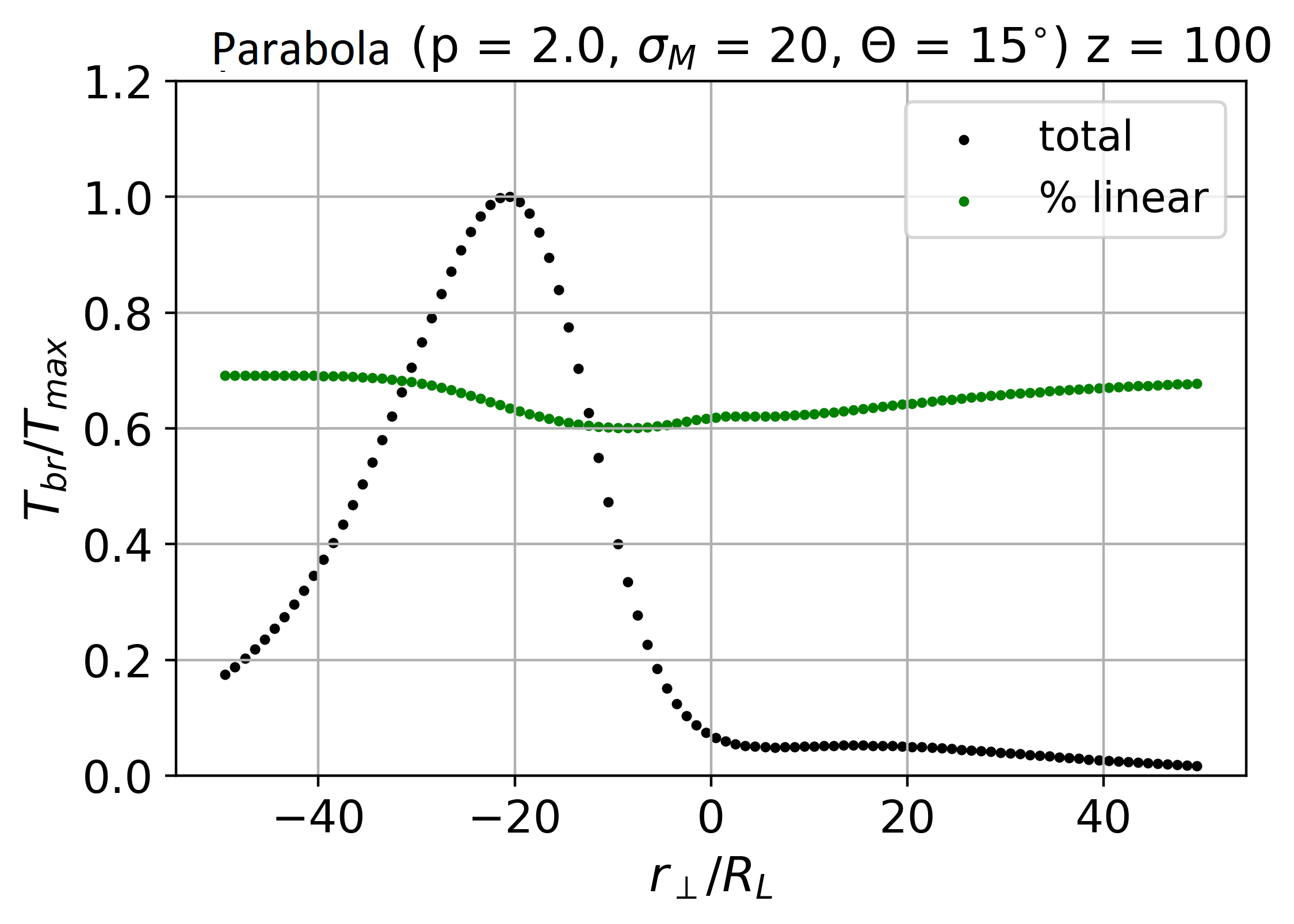
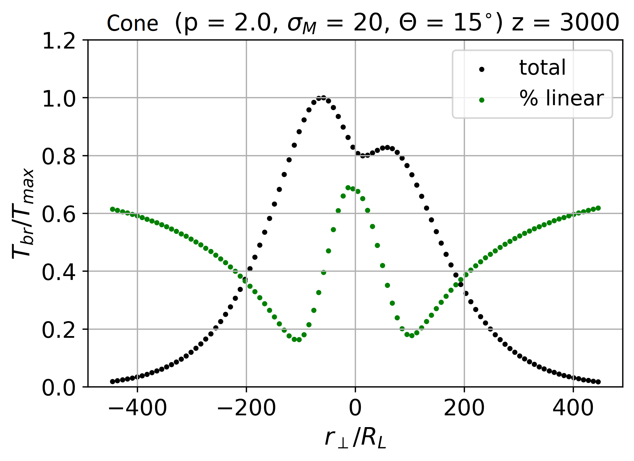
Figure 3: Typical brightness temperature profiles for parabolic and conical flows. The degree of linear polarization at 15 GHz is also shown.

However, a detailed comparison of the theoretical and observed transverse brightness temperature profiles is beyond the scope of this paper; a separate paper will be devoted to such a comparison. Here, having made sure that our results are valid, we consider only the dependence of the brightness temperature $T_{\rm br}$ on the distance $z$ to the central engine. As is usually done, we use the maximum brightness temperature in cross section (i.e., along the so-called ridge line).

Table 1: Exponents $a$ in the relation $T_{\rm br}\propto z^{-a}$ before and after the break for a conical flow for two values of the angle $\Theta$ between the jet axis and the direction to the observer. The jet half-angle is $\theta_{\rm jet}=6^{\circ}$

$\sigma_{\rm M}$	10	20	30	40
$\Theta=2^{\circ}$
$p=2.0$	2.7$-$3.0	3.0$-$3.0	3.3$-$3.0	3.6$-$3.0
$p=2.5$	3.2$-$3.5	3.7$-$3.5	4.0$-$3.5	4.3$-$3.5
$p=3.0$	3.6$-$3.8	4.1$-$3.8	4.4$-$3.8	4.7$-$3.8
$\Theta=20^{\circ}$
$p=2.0$	4.2$-$3.0	5.6$-$3.0	6.2$-$3.0	6.5$-$3.0
$p=2.5$	4.9$-$3.6	6.5$-$3.5	6.7$-$3.6	6.9$-$3.6
$p=3.0$	6.0$-$4.0	7.4$-$4.2	7.7$-$4.3	7.8$-$4.5

Table 2: Exponents $a$ in the relation $T_{\rm br}\propto z^{-a}$ before and after the break for a parabolic flow for two values of the angle $\Theta$ between the jet axis and the direction to the observer.

$\sigma_{\rm M}$	10	20	30	40
$\Theta=2^{\circ}$
$p=2.0$	1.4$-$2.6	1.5$-$3.0	1.5$-$3.0	1.5$-$3.0
$p=2.5$	1.7$-$3.1	1.8$-$3.1	1.8$-$3.1	1.9$-$3.1
$p=3.0$	2.2$-$3.4	2.0$-$3.2	2.0$-$3.2	2.1$-$3.2
$\Theta=20^{\circ}$
$p=2.0$	3.1$-$2.1	2.9$-$2.0	2.9$-$2.0	2.9$-$2.0
$p=2.5$	3.4$-$2.3	3.1$-$2.3	3.1$-$2.3	3.1$-$2.3
$p=3.0$	3.6$-$2.7	3.3$-$2.7	3.3$-$2.7	3.3$-$2.7

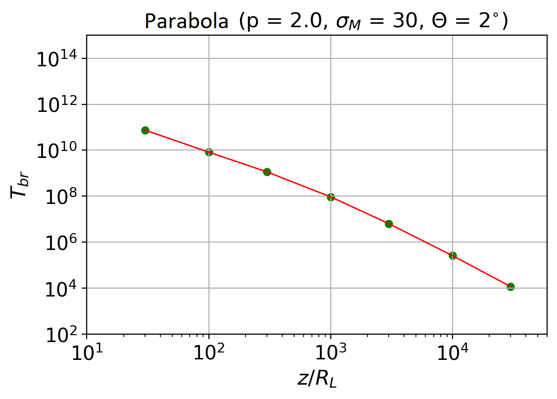
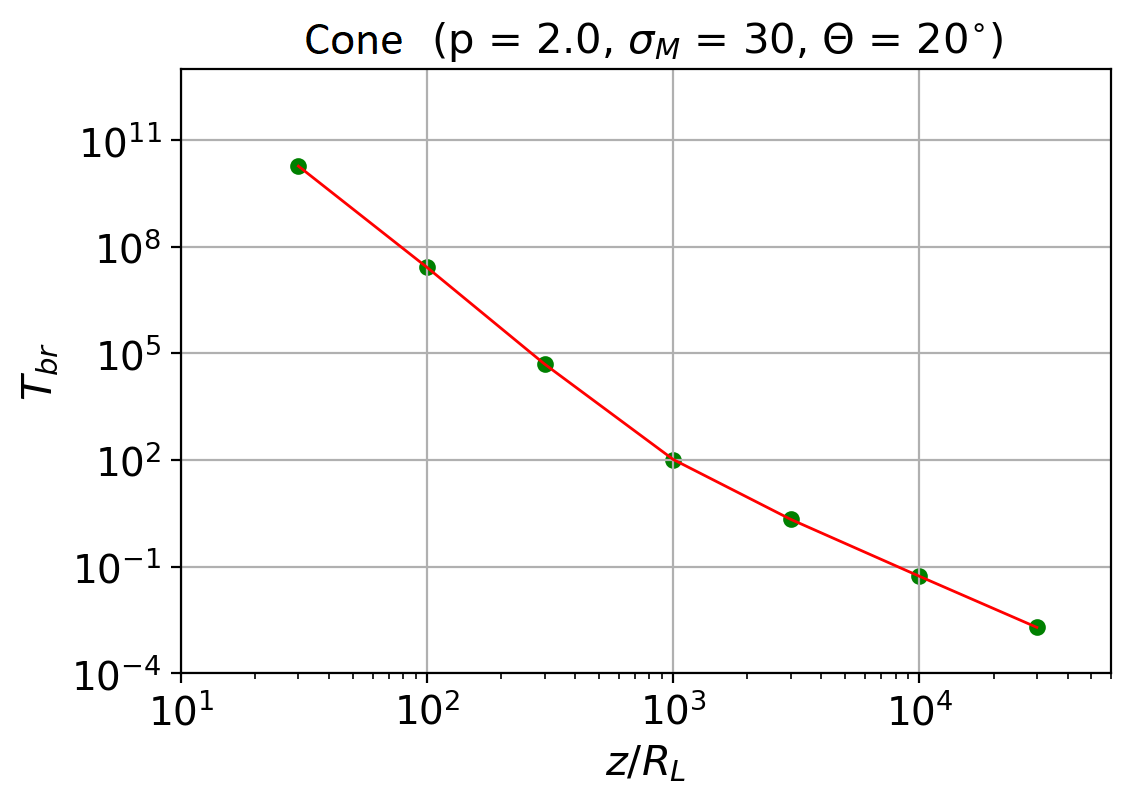
Figure 4: Maximum of the brightness temperature $T_{\rm br}$ (in degrees) versus distance $z$ to the central engine. In both cases, $\lambda_{\gamma}/\lambda=0.001$. For typical black hole masses $\sim 10^{9}M_{\odot}$ and $R_{\rm L}\sim 10r_{\rm g}$ the position of the break corresponds to observed distances $\sim$ 1 pc.

For typical parameters of relativistic jets $\sigma_{\rm M}=20$ and observation angle $\Theta=20^{\circ}$ Fig. 4 shows two examples of the dependence of the brightness temperature $T_{\rm br}$ (in degrees) on the distance to the central engine. For typical black hole masses $\sim 10^{9}M_{\odot}$ and commonly adopted $R_{\rm L}\sim 10\,r_{\rm g}$ the position of the break exactly corresponds to distances $\sim 1$ pc. A full summary of our results for the exponents $a$ in the dependence $T_{\rm br}\propto z^{-a}$ before and after the breakfor two values of the angle $\Theta$ between the jet axis and the direction to the observer is given in Tables 1 and 2. As we see, these dependences do have a break in the saturation region even if the jet geometry does not change in the saturation region. The value of the break itself depends on both spectral index $p$ and magnetization parameter $\sigma_{\rm M}$. The break can be directed both upward and downward. A fortiori there will be a break when passing from a parabolic flow to a conical one. The wide spread of parameters presented in Tables 1 and 2 may well explain the breaks observed in the distance dependence of the brightness temperature in jets.

Yet another important point that should be emphasized here is that to obtain the brightness temperatures corresponding to observations, we set $\lambda_{\gamma}=10^{9}$–$10^{10}$. In other words, to explain the observations, it is sufficient that the energy density of the nonthermal particles be lower than the rest energy density of the cold (background) plasma by two or three orders of magnitude. Thus, the model considered here receives yet another confirmation.

Conclusions

We showed that the conservation of the first adiabatic invariant (i.e., the relationship between the magnetic field in the comoving reference frame $h$ and the energy of radiating particles) naturally leads to a change in the dependence of the brightness temperature $T_{\rm br}$ on the distance $z$ to the central engine, since there are different asymptotic behavior of $h(z)$ before and after the saturation region. This effect was demonstrated for both parabolic and conical relativistic jet structures. Both the presence of a break and the characteristic behavior of the linear polarization qualitatively reproduce the observational data.

Note once again that the goal of this paper was to show only the fundamental possibility of a change in brightness temperature along the jet axis related to the change in the spectrum of radiating particles due to the conservation of the first adiabatic invariant. In contrast, a detailed comparison with observations will become possible only after the refinement of a number of circumstances that were ignored in the above analysis.

This primarily concerns allowance for the transverse inhomogeneity of jets (see, e.g., Nokhrina et al. 2015), which must result in the noticeable fall off of the particle number density and the poloidal magnetic field toward the flow periphery. Accordingly, the dependence of $\sigma_{\rm M}$ (and, hence, the parameter $\varepsilon$) on the distance to the axis should also be taken into account. This can lead to a significant change in brightness temperature. Yet another factor that can also affect quantitatively the results obtained is related to the synchrotron losses. In the Appendix we discussed the losses of particles whose energies correspond to observed frequencies $\sim 10$ GHz. It is clear, however, that the energy losses will be significant for sufficiently high energies of radiating particles, which will lead to a change in the high-energy part of the spectrum. In turn, if the first adiabatic invariant is conserved, at large $z$ this region of the spectrum will already correspond to the observed frequencies. It is not inconceivable that this effect can explain $a>4$ observed in a number of sources. Finally, in this paper we did not discuss the low-frequency self-absorption that can also affect significantly the observed brightness temperature of jets.

Appendix

Above we implicitly assumed that the synchrotron losses of radiating particles could be neglected. Here we will show that this assumption does hold. For this purpose, let us define the quantity $\epsilon$ in the plasma rest frame,

$$\epsilon=\frac{\left({\rm d}\gamma^{\prime}/{\rm d}t^{\prime}\right)_{\rm syn}}{\left({\rm d}\gamma^{\prime}/{\rm d}t^{\prime}\right)_{\rm inv}},$$ (33)

where the derivative

$$\left(\frac{{\rm d}\gamma^{\prime}}{{\rm d}t^{\prime}}\right)_{\rm syn}=\frac{2}{3}\,\frac{e^{4}h^{2}}{m_{\rm e}^{3}c^{5}}\gamma^{2}$$ (34)

corresponds to the synchrotron losses at $\chi=90^{\circ}$, while for any power-law dependences of $h$ on $z$

$$\left(\frac{{\rm d}\gamma^{\prime}}{{\rm d}t^{\prime}}\right)_{\rm inv}\approx\frac{\Gamma c\gamma^{\prime}}{z}.$$ (35)

Here, for simplicity, we substituted ${\rm d}t=\Gamma{\rm d}t^{\prime}$ and $c\,{\rm d}t={\rm d}z$. As a result, we obtain

$$\epsilon\approx\frac{\omega_{h}^{2}r_{\rm e}z\gamma^{\prime}}{\Gamma c^{2}},$$ (36)

where $\omega_{h}=eh/m_{\rm e}c$. To estimate this quantity, it should be remembered that we are interested in the observations at a fixed frequency $\nu\approx\omega_{h}(\gamma^{\prime})^{2}\Gamma$ and, therefore,

$$\epsilon\propto z\,h^{3/2}(z)\Gamma^{-3/2}(z).$$ (37)

As a result, we obtain in the region before the break $x<1/\sqrt{(}2\varepsilon)$ (and neglecting the dependence on $\Gamma$)

$$\epsilon_{\rm conus} \propto z^{-2},$$ (38)

$$\epsilon_{\rm parabolic} \propto z^{-1/2}.$$ (39)

As we see, in both cases the parameter $\epsilon$ decreases with increasing $z$. On the other hand, for $\nu=15$ GHz

$$\epsilon(R_{\rm L})\sim 1\left(\frac{B_{\rm L}}{10^{2}\,G}\right)^{3/2}\left(\frac{R_{\rm L}}{10^{15}\,{\rm cm}}\right).$$ (40)

References

- [1] K. Asada and M. Nakamura, Astrophys. J. Lett. 745, L28 (2012).
- [2] A.-K. Baczko, R. Schulz, M. Kadler, E. Ros, M. Perucho, C. M. Fromm, and J. Wilms, Astron. Astrophys. 623, A27 (2019).
- [3] M. C. Begelman, R. D. Blandford, and M. J. Rees, Rev. Mod. Phys. 56, 255 (1984).
- [4] V. B. Berestetskii, E. M. Lifshitz, and L. P. Pitaevskii, Course of Theoretical Physics, Vol. 4: Quantum Electrodynamics (Nauka, Moscow, 1989; Pergamon, Oxford, 1982).
- [5] V. S. Beskin, Phys. Usp. 53, 1199 (2010).
- [6] V. S. Beskin, MHD Flows in Compact Astrophysical Objects (Fizmatlit, Moscow, 2006; Springer, Heidelberg, 2010).
- [7] R. Blandford, Mon. Not. R. Astron. Soc. 176, 468 (1976).
- [8] B. Boccardi, M. Perucho, C. Casadio, P. Grandi, D. Macconi, E. Torresi, S. Pellegrini, T. P. Krichbaum, M. Kadler, G. Giovannini, V. Karamanavis, L. Ricci, E. Madika, U. Bach, E. Ros, et al., Astron. Astrophys. 647, A67 (2021).
- [9] S. V. Bogovalov, Mon. Not. R. Astron. Soc. 443, 2197 (2014).
- [10] P. R. Burd, M. Kadler, K. Mannheim, A.-K. Baczko, J. Ringholz, and E. Ros, Astron. Astrophys. 660, A1 (2022).
- [11] M. S. Butuzova and A. B. Pushkarev, Mon. Not. R. Astron. Soc. 520, 6335 (2023)
- [12] S. W. Davis and A. D. Tchekhovskoy, Ann. Rev. Astron. Astrophys. 58, 407 (2020).
- [13] D. C. Gabuzda, N. Roche, A. Kirwan, S. Knuettel, M. Nagle, and C. Houston, Mon. Not. R. Astron. Soc. 472, 1792 (2017).
- [14] J. L. Goméz, A. P. Lobanov, G. Bruni, Y. Y. Kovalev, A. P. Marscher, S. G. Jorstad, Yo. Mizuno, U. Bach, R. V. Sokolovsky, J. M. Anderson, P. Galindo, N. S. Kardashev, and M. M. Lisakov, Astrophys. J. 817, 96 (2016).
- [15] J. Heyvaerts and J. Norman, Astrophys. J. 347, 1055 (1989).
- [16] Ya. N. Istomin and V. I. Pariev, Mon. Not. R. Astron. Soc. 281, 1 (1996).
- [17] W. Junor and J. A. Biretta, Astron. J. 109, 500 (1995).
- [18] M. Kadler, E. Ros, A. P. Lobanov, H. Falcke, and J. A. Zensus, Astron. Astrophys. 426, 481 (2004).
- [19] S. Komissarov and O. Porth, New Astron. Rev. 92, 101610 (2021).
- [20] Y. Y. Kovalev, K. I. Kellermann, M. Lister, D. C. Homan, R. C. Vermeulen, M. H. Cohen, E. Ros, M. Kadler, A. P. Lobanov, J. A. Zensus, N. S. Kardashev, L. I. Gurvits, M. F. Aller, and H. D. Aller, Astron. J. 130, 2473 (2005).
- [21] Y. Y. Kovalev, A. V. Pushkarev, E. E. Nokhrina, A. V. Plavin, V.S. Beskin, A. V. Chernoglazov, M. L. Lister, and T. Savolainen, Mon. Not. R. Astron. Soc. 495, 3576 (2020).
- [22] E. V. Kravchenko, Y. Y. Kovalev, and K. V. Sokolovsky, Mon. Not. R. Astron. Soc. 467, 83 (2017).
- [23] L. D. Landau and E. M. Lifshitz, Course of Theoretical Physics, Vol. 2: The Classical Theory of Fields (Nauka, Moscow, 1973; Pergamon, Oxford, 1975).
- [24] A. P. Lobanov and J. A. Zensus, Astrophys. J. 521, 509 (1999).
- [25] A. P. Lobanov, T. P. Krichbaum, D. A. Graham, A. Witzel, A. Kraus, J. A. Zensus, S. Britzen, A. Greve, and M. Grewing, Astron. Astrophys. 364, 391 (2000).
- [26] M. Lyutikov, V. I. Pariev, and R. D. Blandford, Astrophys. J. 597, 998 (2003).
- [27] M. Lyutikov, V. I. Pariev, and D. Gabuzda, Mon. Not. R. Astron. Soc. 360, 869 (2005).
- [28] A. P. Marscher, Astrophys. J. 235, 386 (1980).
- [29] A. P. Marscher and W. K. Gear, Astrophys. J. 298, 114 (1985).
- [30] J. C. McKinney, A. Tchekhovskoy, and R. Blandford, Mon. Not. R. Astron. Soc. 423, 3083 (2012).
- [31] F. C. Michel, Astrophys. J. 158, 727 (1969).
- [32] F. C. Michel, Astrophys. J. 180, L133 (1973).
- [33] M. Mościbrodzka, C. F. Gammie, J.C. Dolence, and H. Shiokawa, Astrophys. J. 735, 9 (2011).
- [34] D. G. Nair, A. P. Lobanov, T. P. Krichbaum, E. Ros, J. A. Zensus, Y. Y. Kovalev, S.-S. Lee, F. Mertens, Yo. Hagiwara, M. Bremer, M. Lindqvist, and P. de Vicente, Astron. Astrophys. 622, A92 (2019).
- [35] E. E. Nokhrina, V. S. Beskin, Y.Y. Kovalev, and A. A. Zheltoukhov, Mon. Not. R. Astron. Soc. 447, 2726 (2015).
- [36] V. I. Pariev, Ya. N. Istomin, and A. R. Beresnyak, Astron. Astrophys. 403, 805 (2003).
- [37] J. Park, K. Hada, M. Nakamura, K. Asada, G. Zhao, and M. Kino, Astrophys. J. 909, 76 (2021).
- [38] G. Pelletier and R. E. Pudritz, Astrophys. J. 394, 117 (1992).
- [39] O. Porth, Ch. Fendt, Z. Meliani, and B. Vaidya, Astrophys. J. 737, 42 (2011).
- [40] V. V. Prokofev, L. I. Arzamasskiy, and V. S. Beskin, Mon. Not. R. Astron. Soc. 454, 2146 (2015).
- [41] K. V. Sokolovsky, Y. Y. Kovalev, A. V. Pushkarev, and A. P. Lobanov, Astron. Astrophys. 532, A38 (2011).
- [42] A. Tchekhovskoy, J. C. McKinney, and R. Narayan, Mon. Not. R. Astron. Soc. 388, 551 (2008).
- [43] C. M. Urry and P. Padovani, Publ. Astron. Soc. Pacif. 107, 803 (1995).
- [44] V. V. Zheleznyakov, Radiation in Astrophysical Plasmas (Yanus-K, Moscow, 1997; Kluwer, Dordrecht, 1996).