Towards Global Solutions for Nonconvex Two-Stage Stochastic Programs: A Polynomial Lower Approximation Approach

Abstract

This paper tackles the challenging problem of finding global optimal solutions for two-stage stochastic programs with continuous decision variables and nonconvex recourse functions. We introduce a two-phase approach. The first phase involves the construction of a polynomial lower bound for the recourse function through a linear optimization problem over a nonnegative polynomial cone. Given the complex structure of this cone, we employ semidefinite relaxations with quadratic modules to facilitate our computations. In the second phase, we solve a surrogate first-stage problem by substituting the original recourse function with the polynomial lower approximation obtained in the first phase. Our method is particularly advantageous for two reasons: it not only generates global lower bounds for the nonconvex stochastic program, aiding in the verification of global optimality for prospective solutions like stationary solutions computed from other methods, but it also simplifies the computation of the expected value of the recourse function by using moments of random vectors. This makes our overall algorithm particularly suitable for the case where the random vector follows a continuous distribution or when dealing with a large number of scenarios. Numerical experiments are conducted to demonstrate the effectiveness of our proposed approach.

Keywords: two-stage stochastic programs, polynomial optimization, nonconvex, global solutions

MSC Classification: 90C23 , 65K05 , 90C15

1 Introduction

Two-stage stochastic programs (SPs) with recourse functions serve as a powerful framework for modeling decision-making problems under uncertainty. In the first stage, “here-and-now” decisions are made prior to the uncertainty being revealed. Following this, the second stage accommodates additional decisions, often contingent on the outcomes of the uncertainty, and are referred as “recourse actions”. The goal of two-stage SPs is to determine decisions that minimize the expected total cost. Mathematically, a two-stage SP with recourse functions is formulated as

$$\left\{\begin{array}[]{cl}\min\limits_{x\in\mathbb{R}^{n_{1}}}&f(x):=f_{1}(x)+\mathbb{E}_{\mu}[f_{2}(x,\xi)]\\[7.22743pt] \mbox{s.t.}&x\in X\,\coloneqq\,\{x\in\mathbb{R}^{n_{1}}:g_{1,i}(x)\geq 0\,(i\in\mathcal{I}_{1})\},\end{array}\right.$$ (1.1)

where $\xi\in\mathbb{R}^{n_{0}}$ is a random vector associated with the probability measure $\mu$ supported on

$$S\,\coloneqq\,\{\xi\in\mathbb{R}^{n_{0}}:g_{0,i}(\xi)\geq 0\,(i\in\mathcal{I}_{0})\},$$ (1.2)

and $f_{2}(x,\xi)$ is the so called recourse function given by:

$$\,\left\{\begin{array}[]{rl}f_{2}(x,\xi):=\min\limits_{y\in\mathbb{R}^{n_{2}}}&F(x,y,\xi)\\[3.61371pt] \mbox{s.t.}&y\in Y(x,\xi)\,\coloneqq\,\{y\in\mathbb{R}^{n_{2}}:g_{2,i}(x,y,\xi)\geq 0\,(i\in\mathcal{I}_{2})\}.\end{array}\right.$$ (1.3)

Herein, $\mathcal{I}_{0},\mathcal{I}_{1}$ and $\mathcal{I}_{2}$ denote finite index sets, potentially empty, and the functions $g_{0,i}:\,\mathbb{R}^{n_{0}}\to\mathbb{R}$ for each $i\in\mathcal{I}_{0}$; $f_{1},\,g_{1,i}:\,\mathbb{R}^{n_{1}}\to\mathbb{R}$ for $i\in\mathcal{I}_{1}$; and $F,\,g_{2,i}:\,\mathbb{R}^{n_{1}}\times\mathbb{R}^{n_{2}}\times\mathbb{R}^{n_{0}}\to\mathbb{R}$ for $i\in\mathcal{I}_{2}$, are all assumed to be real-valued. As a versatile modeling paradigm, two-stage SPs have found applications across numerous domains, such as supply chain management [8, 25], energy systems [6, 28], and transportation planning [17, 34], among others. For a comprehensive understanding of this subject matter, readers are referred to the monographs [1, 41] and references therein.

When $f$ is a convex function and $X$ is a convex set, problem (1.1) is convex. Numerical methods for solving convex two-stage SPs have been extensively studied. When $\xi$ follows a discrete distribution or is approximated by sample averages, (1.1) simplifies to a convex deterministic problem, enabling the application of the $L$-shaped method [43, 44], the (augmented) Lagrangian method [33], and the progressive hedging method [10, 39]. In instances where $\xi$ follows a continuous distribution, one may either directly employ stochastic approximation or utilize sample average approximation to recast it into a deterministic formulation, subsequently applying the aforementioned methods. Under technical assumptions, the (sub)sequences generated by these algorithms converge to globally optimal solutions to the convex SPs.

Many real-world applications feature two-stage SPs that are inherently nonconvex. Examples include the two-stage stochastic interdiction problem [4, 12] and the stochastic program with decision-dependent uncertainty [9, 14, 23, 24, 36]. In fact, the recourse function in the form of (1.3) easily becomes nonconvex in the first-stage variable $x$, even in the simple situation where the second-stage problem is linearly parameterized by $x$:

$$\,\left\{\begin{array}[]{rl}f_{2}(x,\xi)=\min\limits_{y\in\mathbb{R}^{n_{2}}}&[\,c(\xi)+C(\xi)x\,]^{T}y\\[3.61371pt] \mbox{s.t.}&A(\xi)x+B(\xi)y\geq b(\xi).\end{array}\right.$$

It is important to note that the nonconvexity in the above problem does not arise from the integrality of decision variables $y$, and thus techniques from the mixed-integer programming is not applicable here. For such problems, the focus in the existing literature is primarily on the efficient computation of local solutions, such as stationary points [2, 23, 24]. Generally, it is challenging to compute global optimal solutions of nonconvex two-stage SPs as well as to certify the quality of a given point in terms of its global optimality.

The primary goal of the present paper is to design a relaxation approach that can asymptotically solve problem (1.1) to global optimality, under the setting that the recourse function $f_{2}$ is nonconvex in $x$. One major challenge in globally solving (1.1) stems from the typical lack of an explicit parametric representation of the recourse function $f_{2}(x,\xi)$. To overcome this difficulty, we introduce a two-phase algorithm. In the first phase, we construct a parametric function $p(x,\xi)$ that serves as a lower approximation of the recourse function $f_{2}(x,\xi)$ over $X\times S$, satisfying

$$f_{2}(x,\xi)-p(x,\xi)\geq 0,\quad\forall\,x\in X,\,\xi\in S.$$ (1.4)

In the second phase, we replace $f_{2}(x,\xi)$ in problem (1.1) with the approximating function $p(x,\xi)$ and solve the corresponding surrogate problem to global optimality. Given that $p$ provides a lower approximation of $f_{2}$ on its domain, the global optimal value computed from the surrogate problem must be a lower bound of the true optimal value of problem (1.1). Consequently, this computed value also provides an estimate of the distance from the objective value at a local solution/stationary point that is obtained by any other methods to the true global optimal value. In addition, we design a hierarchical procedure to asymptotically diminish the gap between $f_{2}(x,\xi)$ and $p(x,\xi)$ (in the ${\cal L}^{1}$ space), thereby ensuring that the objective value obtained from the surrogate problem converges to the true global optimal value of (1.1).

To achieve our goal of finding the global optimal solution of the nonconvex two-stage SP, we leverage techniques from polynomial optimization. It is well known that under the archimedean condition, a generic polynomial optimization problem can be solved to global optimality through a hierarchy of Moment-Sum-of-Squares (Moment-SOS) relaxations [20]; see, for example, the monographs [21, 22, 31]. Specifically, let us denote

$$\mathcal{F}\,\coloneqq\,\{(x,\xi)\in X\times S:Y(x,\xi)\neq\emptyset\}\quad\mbox{and}\quad K\,\coloneqq\,\{(x,y,\xi):(x,\xi)\in\mathcal{F},y\in Y(x,\xi)\}.$$ (1.5)

Then for any $(x,\xi)\in\mathcal{F}$, the inequality (1.4) is equivalent to

$$F(x,y,\xi)-p(x,\xi)\geq 0,\quad\forall\,y\in Y(x,\xi).$$ (1.6)

Assuming that the functions $F$ and $g_{2,i}$ for $i\in{\cal I}_{2}$ in (1.3) are polynomials over $(x,y,\xi)$, we construct a polynomial function $p(x,\xi)$ such that $F(x,u,\xi)-p(x,\xi)$ is a nonnegative polynomial over $K$. Obviously there are infinitely many polynomials satisfying the above condition. In order to approximate the recourse function $f_{2}(x,\xi)$ as tight as possible, we seek the one that is closest to it from below under a prescribed metric. Specifically, letting $\mathscr{P}(K)$ be the set of polynomials in $(x,y,\xi)$ that are nonnegative on $K$ and $\nu$ be a probability measure supported on $\mathcal{F}$, we solve for a best polynomial lower approximating function via the following problem

$$\left\{\begin{array}[]{cl}\max\limits_{p}&\int_{\mathcal{F}}p(x,\xi){\tt d}\nu\\ \mbox{s.t.}&F(x,y,\xi)-p(x,\xi)\in\mathscr{P}(K).\end{array}\right.$$ (1.7)

When the degree of the polynomial $p(x,\xi)$ is fixed, the above problem reduces to a linear conic optimization in the coefficients of $p$. A noteworthy benefit of problem (1.7) is that the size of the decision variables are determined merely by the dimensions of $(x,\xi)$ and the degree of the polynomial $p$, while remaining unaffected by the distribution of $\xi$ or the number of samples used to approximate $\xi$’s distribution. This becomes particularly advantageous when there is a large number of scenarios for $\xi$. Even more appealingly, if $\xi$ follows a continuous distribution, there is no necessity to draw samples to approximate its distribution in order to compute $\mathbb{E}_{\nu}[\,p(x,\xi)\,]$; it can instead be computed analytically through the moments of $\xi$.

Figure 1: An illustration of our approach. The left panel shows how a nonconvex recourse function $f(x,\xi)$ can be efficiently approximated from below by a polynomial $p(x,\xi)$. The right panel shows the expectation of the recourse and its approximation from the left (i.e., $\mathbb{E}_{\nu}[f(x,\xi)]$ vs $\mathbb{E}_{\nu}[p(x,\xi)]$) for a given measure $\nu$.

We outline the major advantages of our proposed approach below.

• Our method efficiently computes lower bounds for the global optimal value of problem (1.1), which can be particularly tight when the recourse function is polynomial. These bounds can be used to certify the global optimality of prospective solutions like stationary solutions computed from other methods.

• The approach yields an explicit polynomial lower bound for the recourse function. With certain assumptions of compactness and continuity, these polynomials can achieve an arbitrarily level of accuracy in the $\mathcal{L}^{1}$ space relative to a given probability measure.

• The number of variables in problem (1.7) is independent of the distribution of $\xi$. Therefore, our approach is especially beneficial in instances where $\xi$ follows a continuous distribution or is approximated by a large number of scenarios.

The rest of this paper is organized as follows. Some notation and basic knowledge on polynomial optimization is introduced right after. In section 2, we discuss the construction of polynomial lower approximation of the recourse function via linear conic optimization. Utilizing the derived polynomial lower approximating functions, we develop algorithms to approximately solve nonconvex two-stage SPs in section 3, and study their convergent properties. In section 4, the Moment-SOS relaxation methods are introduced to solve the subproblems arising from the algorithms in the previous section. Some numerical results are given in section 5. The paper ends with a concluding section.

Notation and Preliminaries

The symbol $\mathbb{R}$ denotes the set of real numbers and $\mathbb{N}$ denotes the set of nonnegative integers. The notation $\mathbb{R}^{n}$ (resp., $\mathbb{N}^{n}$) stands for the set of $n$-dimensional vectors with entries in $\mathbb{R}$ (resp., $\mathbb{N}$). For $t\in\mathbb{R}$, $\lceil t\rceil$ denotes the smallest integer that is not smaller than $t$. For an integer $k>0$, denote $[k]\coloneqq\{1,\cdots,k\}$. For a vector $v\in\mathbb{R}^{n}$, we use $\|v\|$ to denote its Euclidean norm. The superscript ^T denotes the transpose of a matrix or vector. Let $\Omega_{1}$ and $\Omega_{2}$ be two sets. Their Cartesian product is denoted as $\Omega_{1}\times\Omega_{2}\,\coloneqq\,\{(v_{1},v_{2}):\,v_{1}\in\Omega_{1},\,v_{2}\in\Omega_{2}\}$. Let $\nu$ be a probability measure supported on $\Omega_{1}$ and $\mathcal{L}^{1}(\nu)$ denote the set of functions $f:\Omega_{1}\to\mathbb{R}$ such that $\int_{\Omega_{1}}|f|{\tt d}\nu<\infty$. A matrix $A\in\mathbb{R}^{n\times n}$ is said to be positive semidefinite, denoted as $A\succeq 0$, if $v^{T}Av\geq 0$ for all $v\in\mathbb{R}^{n}$. If $v^{T}Av>0$ for every nonzero vector $v\in\mathbb{R}^{n}$, then $A$ is positive definite, written as $A\succ 0$. Let $w=(w_{1},\ldots,w_{\ell})$ be a vector of variables. We use $\mathbb{R}[w]$ to denote the ring of real polynomials in $w$. Then $\mathbb{R}[w]_{d}\subseteq\mathbb{R}[w]$ is the set of real polynomials with degrees no more than $d$. For a polynomial $f(x,y,\xi)$, its total degree is denoted by $\deg(f)$. We use $\deg_{x}(f)$ (resp., $\deg_{y}(f)$, $\deg_{\xi}(f)$) to denote its partial degree in $x$ (resp., $y$, $\xi$). For a tuple of polynomials $h=(h_{1},\ldots,h_{m})$, the notation $\deg(h)$ represents the highest degree among all $h_{i}$’s. For a monomial power $\alpha\coloneqq(\alpha_{1},\ldots,\alpha_{\ell})\in\mathbb{N}^{\ell}$, denote

$$w^{\alpha}\,\coloneqq\,w_{1}^{\alpha_{1}}\cdots w_{\ell}^{\alpha_{\ell}},\quad\mbox{with}\quad|\alpha|\,\coloneqq\,\alpha_{1}+\cdots+\alpha_{\ell}.$$

For a degree $d$, denote the set of monomial powers in $w$ as $\mathbb{N}_{d}^{\ell}\,\coloneqq\,\{\alpha\in\mathbb{N}^{\ell}:|\alpha|\leq d\}$. The notation

$$[w]_{d}\,\coloneqq\,\begin{bmatrix}1&w_{1}&\cdots&w_{\ell}&(w_{1})^{2}&w_{1}w_{2}&\cdots&(w_{\ell})^{d}\end{bmatrix}^{T},$$

denotes the monomial vector with the highest degree $d$ and ordered alphabetically.

A polynomial $p\in\mathbb{R}[w]$ is said to be a sum-of-squares (SOS) if it can be expressed as $p=p_{1}^{2}+\cdots+p_{t}^{2}$ for some $p_{1},\ldots,p_{t}\in\mathbb{R}[w]$. The set of all SOS polynomials in $w$ is denoted by $\Sigma[w]$. Its $d$th degree truncation is denoted by $\Sigma[w]_{d}\coloneqq\Sigma[w]\cap\mathbb{R}[w]_{d}$. Let $h=(h_{1},\ldots,h_{m})$ be a tuple of polynomials and define $\Omega=\{w\in\mathbb{R}^{\ell}:h(w)\geq 0\}$. We denote the nonnegative polynomial cone over $\Omega$ as

$$\mathscr{P}(\Omega)\,\coloneqq\,\{p\in\mathbb{R}[w]:p(w)\geq 0,\forall w\in\Omega\}.$$

For every degree $d$, $\mathscr{P}_{d}(\Omega)\,\coloneqq\,\mathscr{P}(\Omega)\cap\mathbb{R}[w]_{d}$. The preordering of $h$ is given as

$$\mathit{Pre}[h]\,\coloneqq\,\sum\limits_{J\subseteq[m]}\Big{(}\prod\limits_{i\in J}h_{i}\Big{)}\cdot\Sigma[w].$$ (1.8)

Clearly, $\mathit{Pre}[h]\subseteq\mathscr{P}(\Omega)$. Interestingly, when $\Omega$ is compact, every polynomial that is positive on $\Omega$ belongs to $\mathit{Pre}[h]$. This conclusion is referenced as Schmudgen’s Positivstellensatz [35]. The quadratic module of $h$ is a subset of $\mathit{Pre}[h]$, which is defined as

$$\mathit{QM}[h]\,\coloneqq\,\Sigma[w]+h_{1}\cdot\Sigma[w]+\cdots+h_{m}\cdot\Sigma[w].$$

Its $k$th order truncation is given as

$$\mathit{QM}[h]_{2k}\,\coloneqq\,\Sigma[w]_{2k}+h_{1}\cdot\Sigma[w]_{2k-\deg(h_{1})}+\cdots+h_{m}\cdot\Sigma[w]_{2k-\deg(h_{m})}.$$ (1.9)

When $\Omega$ is compact, $\mathit{QM}[h]$ and each $\mathit{QM}[h]_{2k}$ are closed convex cones. For every $k$ such that $2k\geq\deg(h)$, the nested containment relation holds that

$$\mathit{QM}[h]_{2k}\,\subseteq\,\mathit{QM}[h]_{2k+2}\,\subseteq\,\cdots\,\subseteq\,\mathit{QM}[h]\,\subseteq\,\mathit{Pre}[h]\,\subseteq\,\mathscr{P}(\Omega).$$

In particular, $\mathit{QM}[h]$ is said to be archimedean if there exists $q\in\mathit{QM}[h]$ such that $q(w)\geq 0$ determines a compact set. Suppose $\mathit{QM}[h]$ is archimedean. Every polynomial that is positive on $\Omega$ must be contained in $\mathit{QM}[h]$. This conclusion is called Putinar’s Postivstellensatz [35]. It is clear that $\Omega$ is compact when $\mathit{QM}[h]$ is archimedean. Conversely, if $\Omega$ is compact, $\mathit{QM}[h]$ may not be archimedean. In this case, we can always find a sufficiently large $R>0$ such that $\Omega$ is contained in $\{w:R-\|w\|^{2}\geq 0\}$ and that $\mathit{QM}[\tilde{h}]$ is archimedean for $\tilde{h}=(h,R-\|w\|^{2})$.

For an integer $k\geq 0$, a real vector $z=(z_{\alpha})_{\alpha\in\mathbb{N}_{2k}^{\ell}}$ is said to be a truncated multi-sequence (tms) of $x$ with degree $2k$. For a polynomial $p(x)=\sum_{\alpha\in\mathbb{N}^{\ell}_{2k}}p_{\alpha}x^{\alpha}$, denote the bilinear operation in $p$ and $z$ as:

$$\langle p,z\rangle\,\coloneqq\,{\sum}_{\alpha\in\mathbb{N}^{\ell}_{2k}}p_{\alpha}z_{\alpha}.$$ (1.10)

For a polynomial $q\in\mathbb{R}[x]_{2t}$ with $t\leq k$, the $k$th order localizing matrix of $q$ and $z$ is the symmetric matrix $L_{q}^{(k)}[z]$ that satisfies

$$\langle qa^{2},z\rangle\,=\,vec(a)^{T}\big{(}L_{q}^{(k)}[z]\big{)}vec(a)$$ (1.11)

for each polynomial $a(x)=vec(a)^{T}[x]_{s}$ with $s\leq k-t$. When $q=1$ being the constant one polynomial, $L_{q}^{(k)}[z]$ becomes the $k$th order moment matrix $M_{t}[z]\coloneqq L_{1}^{(k)}[z]$. Quadratic modules and their dual cones play a critical role in polynomial optimization. Recently, polynomial optimization has been actively studied in [18, 19, 27, 37]. We refer to monographs [21, 22, 31] for comprehensive results in polynomial optimization.

2 Lower Approximations of Recourse Functions via Polynomials

This section is devoted to the phase one of our approach on the construction of a polynomial lower approximation of the (nonconvex) recourse function $f_{2}(x,\xi)$ over ${\cal F}$, under the assumption that the functions $F(x,y,\xi)$, $\{g_{2,i}(x,y,\xi)\}$ and $\{g_{0,i}(\xi)\}$ in problems (1.1) and (1.2) are polynomials.

2.1 Linear conic optimization

In this subsection, we discuss how to solve problem (1.7). This is a linear conic optimization problem whose decision variable is the coefficient vector of $p(x,\xi)$. We start with a toy example.

Example 2.1.

Let $x,y,\xi\in\mathbb{R}$ and

$$F(x,y,\xi)=(x+y-\xi)^{2},\quad X=S=\mathbb{R},\quad Y(x,\xi)=Y=\mathbb{R}.$$

Obviously $\mathcal{F}=\mathbb{R}^{2}$ and $K=\mathbb{R}^{3}$. We take $\nu$ as the standard normal distribution on $\mathbb{R}^{2}$ and $p(x,\xi)$ as a quadratic polynomial in the form of

$$p(x,\xi)\,=\,p_{00}+p_{10}x+p_{01}\xi+p_{20}x^{2}+p_{11}x\xi+p_{02}\xi^{2}.$$

Since $\int_{\mathcal{F}}x{\tt d}\nu=\int_{\mathcal{F}}\xi{\tt d}\nu=\int_{\mathcal{F}}x\xi{\tt d}\nu=0$ and $\int_{\mathcal{F}}1{\tt d}\nu=\int_{\mathcal{F}}x^{2}{\tt d}\nu=\int_{\mathcal{F}}\xi^{2}{\tt d}\nu=1$, we have

$$\int_{\mathcal{F}}p(x,\xi){\tt d}\nu\,=\,p_{00}+p_{20}+p_{02}.$$

In addition, since $\mathscr{P}_{2}(\mathbb{R}^{3})=\Sigma[x,y,\xi]_{2}$, we have that

$$F(x,y,\xi)-p(x,\xi)\,=\,\begin{bmatrix}1\\ x\\ y\\ \xi\end{bmatrix}^{T}\left[\begin{array}[]{rrrr}-p_{00}&-0.5p_{10}&0&-0.5p_{01}\\ -0.5p_{10}&1-p_{20}&1&-1-0.5p_{11}\\ 0&1&1&-1\\ -0.5p_{01}&-1-0.5p_{11}&-1&1-p_{02}\end{array}\right]\begin{bmatrix}1\\ x\\ y\\ \xi\end{bmatrix}$$

is nonnegative on $\mathbb{R}^{3}$ if and only if the above coefficient matrix is positive semidefinite. This is satisfied when all coefficients of $p(x,\xi)$ are zeros, i.e., $p=0$ is the identically zero polynomial.

In general, even if all the functions $F(x,y,\xi)$ and $g_{2,i}(x,y,\xi)$ for $i\in{\cal I}_{2}$ in (1.3) are polynomials, the value function $f_{2}(x,\xi)$ may not be continuous, as can be seen from the following example ($x,y,\xi$ are all univariate):

$$\left(\begin{array}[]{ll}f_{2}(x,\xi)=&\displaystyle\min_{y}\;y\\ &\mbox{s.t.}\quad xy=0,\;-1\leq y\leq\xi^{2}.\end{array}\right)=\left\{\begin{array}[]{ll}-1&\mbox{if $x=0$,}\\[1.4457pt] 0&\mbox{if $x\neq 0$.}\end{array}\right.$$

Additional assumptions are needed to make the function $f_{2}$ continuous, such as the restricted inf-compactness condition [11, Definition 3.13] together with some constraint qualifications. We refer to [3, §6.5.1] and [7, 38] for more details on these results. When $\mathcal{F}$ is compact and the value function $f_{2}(x,\xi)$ is continuous, the objective in (1.7) is bounded from above and its optimal value equals the integral of $f_{2}(x,\xi)$ with respect to $\nu$. We formally state the results below.

Theorem 2.2.

Assume $\mathcal{F}$ is compact and $f_{2}(x,\xi)$ is continuous on $\mathcal{F}$. For a given probability measure $\nu$ supported on $\mathcal{F}$, the objective in (1.7) is bounded from above on its feasible region and the optimal value equals $\int_{\mathcal{F}}f_{2}(x,\xi){\tt d}\nu$.

Proof.

Under the given assumptions, the integral $\int_{\mathcal{F}}f_{2}(x,\xi){\tt d}\nu$ is finite and it is an upper bound for the optimal value of (1.7). Let $\varepsilon>0$ be an arbitrarily small scalar. By Weierstrass approximation theorem [40, Theorem 7.26], there is a polynomial $q_{\varepsilon}\in\mathbb{R}[x,\xi]$ such that

$$|f_{2}(x,\xi)-q_{\varepsilon}(x,\xi)|\,\leq\,\varepsilon,\quad\forall(x,\xi)\in\mathcal{F}.$$

Let $\tilde{q}_{\varepsilon}(x,\xi)\coloneqq q_{\varepsilon}(x,\xi)-\varepsilon$. It is feasible for (1.7) because for every triple $(x,y,\xi)\in K$, we have

$$F(x,y,\xi)-\tilde{q}_{\varepsilon}(x,\xi)\,\geq\,(f_{2}(x,\xi)-q(x,\xi))+\varepsilon\,\geq\,0.$$

In addition, for the given probability measure $\nu$, since $\int_{\mathcal{F}}1{\tt d}\nu=1$, it holds that

$$\int_{\mathcal{F}}|f_{2}(x,\xi)-\tilde{q}_{\varepsilon}(x,\xi)|{\tt d}{\nu}\,\leq\,\max\limits_{(x,\xi)\in\mathcal{F}}\,|f_{2}(x,\xi)-q_{\varepsilon}(x,\xi)|+\varepsilon\,\leq\,2\varepsilon.$$

Since $\varepsilon$ can be arbitrarily small, there exists a sequence of optimizing polynomials converging to $f_{2}(x,\xi)$ in $\mathcal{L}^{1}(\nu)$. Hence, their integrals converge to $\int_{\mathcal{F}}f_{2}(x,\xi){\tt d}\nu$. ∎

When the recourse function $f_{2}(x,\xi)$ is itself a polynomial, problem (1.7) has a global optimal solution $f_{2}(x,\xi)$. If, however, the function $f_{2}(x,\xi)$ is not a polynomial, we can construct a sequence of approximating polynomial functions $\{p^{(k)}\}_{k=1}^{\infty}$, each serving as a lower bound for $f_{2}(x,\xi)$ over ${\cal F}$. Furthermore, the integral $\int_{\mathcal{F}}p^{(k)}(x,\xi)\,{\tt d}\nu$ converges to the optimal value of (1.7) as $k\to\infty$. In section 4, we will discuss how to compute such a convergent polynomial sequence numerically.

Suppose $\{p^{(k)}(x,\xi)\}_{k=1}^{\infty}$ is an optimizing sequence of (1.7), i.e., each of them is feasible to (1.7) and $\displaystyle\lim_{k\to\infty}\int_{\mathcal{F}}p^{(k)}(x,\xi){\tt d}\nu=\int_{\mathcal{F}}f_{2}(x,\xi){\tt d}\nu$. Then the term $\mathbb{E}_{\mu}[f_{2}(x,\xi)]$, which is the expectation of the recourse function in the first stage problem (1.1), should be well approximated by $\mathbb{E}_{\mu}[p^{(k)}(x,\xi)]$ when $k$ is sufficiently large. The accuracy of the estimation depends on the selection of the probability measure $\nu$. For instance, if $\nu$ is the uniform distribution over $\mathcal{F}$, then (1.7) finds a lower approximating function that uniformly approximates $f_{2}(x,\xi)$ across $\mathcal{F}$. If we define $\nu\coloneqq\delta_{\hat{x}}\times\mu$, where $\delta_{\hat{x}}$ is a Dirac measure centered at $\hat{x}\in X$, and $S$ denotes the projection of $\mathcal{F}$ onto the $\xi$-plane, then the objective of (1.7) reduces to

$$\int_{\mathcal{F}}p(x,\xi){\tt d}(\delta_{\hat{x}}\times\mu)\,=\,\int_{S}p(\hat{x},\xi){\tt d}\mu\,=\,\mathbb{E}_{\mu}[p(\hat{x},\xi)].$$

Solving (1.7) gives an accurate evaluation of $\mathbb{E}_{\mu}[p(x,\xi)]$ at the point $x=\hat{x}$. In practice, we can strategically modify the measure $\nu$ to enhance the approximation of the original function in specific areas. Further discussions of this approach are given in the next section.

The requirement for $f_{2}(x,\xi)$ being continuous over $\mathcal{F}$ can be relaxed to being integrable with respect to the Lebesgue-Stieltjes measure $\nu$. This relaxed condition allows for the inclusion of functions that may possess discontinuities yet remain integrable. The formal statement and proof of this relaxation are given in the following corollary.

Corollary 2.3.

(a) If $f_{2}(x,\xi)$ is a polynomial, then it must be a global optimal solution of (1.7).

(b) Suppose $\mathcal{F}$ is compact and $\nu$ is a Lebesgue-Stieltjes probability measure supported on $\mathcal{F}$. If $f_{2}(x,\xi)\in\mathcal{L}^{1}(\nu)$, then the problem (1.7) is bounded from above, and its optimal value is equal to $\int_{\mathcal{F}}f_{2}(x,\xi){\tt d}\nu$.

Proof.

Part (a) is obvious. For part (b), when $\mathcal{F}$ is compact and $\nu$ is a Lebesgue-Stieltjes measure, the set of continuous functions is dense in $\mathcal{L}^{1}(\nu)$. Therefore, the result can be proved via similar arguments in the proof of Theorem 2.2. ∎

2.2 A special case: $\xi$ has a finite support

When the random vector $\xi$ has a finite support, say $S=\{\xi^{(1)},\ldots,\xi^{(r)}\}$, we may approximate the recourse function $f_{2}(x,\xi)$ at each $\xi^{(i)}$ individually by a polynomial merely in terms of $x$ to enhance the quality of the overall approximations. Specifically, assume

$$\mu\,=\,\lambda_{1}\delta_{\xi^{(1)}}+\lambda_{2}\delta_{\xi^{(2)}}+\cdots+\lambda_{r}\delta_{\xi^{(r)}},$$ (2.1)

where each $\lambda_{i}>0$ and that $\lambda_{1}+\lambda_{2}+\cdots+\lambda_{r}=1$. In this setting, the expected recourse can be expressed as

$$\mathbb{E}_{\mu}[f_{2}(x,\xi)]\,=\,\lambda_{1}f_{2}(x,\xi^{(1)})+\lambda_{2}f_{2}(x,\xi^{(2)})+\cdots+\lambda_{r}f_{2}(x,\xi^{(r)}).$$

In the above, every $f_{2}(x,\xi^{(i)})$ is a function only dependent on $x$. Note that $f_{2}(x,\xi^{(i)})\leq F(x,y,\xi^{(i)})$ for every $y\in Y(x,\xi^{(i)})$. Since $F(x,y,\xi^{(i)})$ is a polynomial, when $X$ is compact, the function $f_{2}(x,\xi^{(i)})$ is bounded from above over the set

$$\mathcal{F}_{i}\coloneqq\{x\in X:Y(x,\xi^{(i)})\not=\emptyset\}.$$ (2.2)

The feasible region in (1.5) becomes $\mathcal{F}=\bigcup_{i=1}^{r}\mathcal{F}_{i}\times\{\xi^{(i)}\}$. If for every $i\in[r]$, we can find a polynomial $p_{i}\in\mathbb{R}[x]$ such that

$$f_{2}(x,\xi^{(i)})-p_{i}(x)\,\geq\,0,\quad\forall x\in\mathcal{F}_{i},$$ (2.3)

then a lower approximating function for the expected recourse can be constructed as

$$p(x)\,\coloneqq\,\lambda_{1}p_{1}(x)+\lambda_{2}p_{2}(x)+\cdots+\lambda_{r}p_{r}(x).$$ (2.4)

Consequently, $\mathbb{E}_{\mu}[f_{2}(x,\xi)]-p(x)\,\geq\,0$ for any $x\in X$. Such polynomials $p_{i}(x)$ can be solved via linear conic optimization problems similarly as in the previous subsection. Let $\nu_{i}$ be a probability measure supported on $\mathcal{F}_{i}$ and denote the feasible region

$$K_{i}\,\coloneqq\,\big{\{}(x,y):x\in\mathcal{F}_{i},\,y\in Y(x,\xi^{(i)})\big{\}}.$$ (2.5)

Consider the optimization problem

$$\left\{\begin{array}[]{cl}\max\limits_{p_{i}\in\mathbb{R}[x]}&\int_{\mathcal{F}_{i}}p_{i}(x){\tt d}\nu_{i}\\ \mbox{s.t.}&F(x,y,\xi^{(i)})-p_{i}(x)\in\mathscr{P}(K_{i})^{x,y},\end{array}\right.$$ (2.6)

where $\mathscr{P}(K_{i})^{x,y}\coloneqq\{q\in\mathbb{R}[x,y]:q(x,y)\geq 0,\forall(x,y)\in K_{i}\}$ is the nonnegative polynomial cone. To emphasize $\mathscr{P}(K_{i})^{x,y}\subseteq\mathbb{R}[x,y]$, we add the superscript ^x,y to distinguish it from $\mathscr{P}(K)\subseteq\mathbb{R}[x,y,\xi]$. Clearly, every feasible polynomial of (2.6) satisfies (2.3). Problem (2.6) aims to find the best polynomial lower approximating function of $f_{2}(x,\xi^{(i)})$ such that

$$\int_{\mathcal{F}_{i}}|f_{2}(x,\xi^{(i)})-p_{i}(x)|{\tt d}\nu_{i}\,=\,\int_{\mathcal{F}_{i}}f_{2}(x,\xi^{(i)}){\tt d}\nu_{i}-\int_{\mathcal{F}_{i}}p_{i}(x){\tt d}\nu_{i}$$

is minimized. Compared to problem (1.7), problem (2.6) has a smaller number of variables, which is expected to be easier to solve in practice. It has computational advantages when the cardinality of the support set $S$ is small but the dimension for the random vector $\xi$ is large. Indeed, to solve for a polynomial lower bound function of degree $d$, the number of variables in (1.7) is $\binom{n_{0}+n_{1}+d}{d}$ and the number of variables in (2.6) is $\binom{n_{1}+d}{d}$. In applications, the finite support $S$ is usually not given directly but is approximated by a large number of samples. In this case, we can apply the method proposed in [32] to find a finite set $\tilde{S}$ that is close to $S$. A group of lower approximating function $\tilde{p}_{i}(x)$ can be similarly computed by solving (2.6) with respect to each scenario in $\tilde{S}$. When $\tilde{S}$ is sufficiently close to $S$, such $\tilde{p}_{i}(x)$ can also be used to form a good approximation of the recourse function.

Under some compact and continuous assumptions, we can obtain similar results to Theorem 2.2.

Theorem 2.4.

Assume $\mathcal{F}_{i}$ is compact and $f_{2}(x,\xi^{(i)})$ is continuous on $\mathcal{F}_{i}$. For a given probability measure $\nu_{i}$ supported on $\mathcal{F}_{i}$, problem (2.6) is bounded from above and its optimal value is $\int_{\mathcal{F}_{i}}f_{2}(x,\xi^{(i)}){\tt d}\nu_{i}$.

Proof.

Under given assumptions, the integral $\int_{\mathcal{F}_{i}}f_{2}(x,\xi){\tt d}\nu_{i}$ is finite and $\int_{\mathcal{F}_{i}}f_{2}(x,\xi){\tt d}\nu_{i}\geq\int_{\mathcal{F}_{i}}p(x){\tt d}{\nu_{i}}$ for every feasible polynomial of (2.6). By Weierstrass approximation theorem [40, Theorem 7.26], for every $\varepsilon>0$, there exists a real polynomial $q_{\varepsilon}(x)$ such that

$$|f_{2}(x,\xi^{(i)})-q_{\varepsilon}(x)|\,\leq\,\varepsilon,\quad\forall x\in\mathcal{F}_{i}.$$

Let $\tilde{q}_{\varepsilon}(x)\coloneqq q_{\varepsilon}(x)-\varepsilon$. It is feasible for (2.6) and satisfies

$$\int_{\mathcal{F}_{i}}|f_{2}(x,\xi^{(i)})-\tilde{q}_{\varepsilon}(x)|{\tt d}\nu_{i}\,\leq\,\max\limits_{x\in\mathcal{F}_{i}}\,|f_{2}(x,\xi^{(i)})-q_{\varepsilon}(x)|+\varepsilon\,\leq\,2\varepsilon.$$

Since $\varepsilon$ can be arbitrarily small, there exists a sequence of feasible optimizing polynomials that converges to $f_{2}(x,\xi^{(i)})$ in $\mathcal{L}^{1}(\nu_{i})$, with their integrals converging to $\int_{\mathcal{F}_{i}}f_{2}(x,\xi^{(i)}){\tt d}\nu_{i}$. ∎

As in Corollary 2.3, the continuous assumption of $f_{2}(x,\xi^{(i)})$ can be relaxed when $\nu_{i}$ is a Lebesgue-Stieltjes measure.

Corollary 2.5.

(a) If $f_{2}(x,\xi^{(i)})$ is a polynomial, then it must be an optimizer of (2.6).

(b) Suppose $\mathcal{F}_{i}$ is compact and $\nu_{i}$ is a Lebesgue-Stieltjes measure supported on $\mathcal{F}_{i}$. If $f_{2}(x,\xi)\in\mathcal{L}^{1}(\nu_{i})$, then problem (2.6) is bounded from above and its optimal value is $\int_{\mathcal{F}_{i}}f_{2}(x,\xi^{(i)})$.

2.3 Conditions on tight lower bounds

A polynomial lower approximating function $p(x,\xi)$ is said to be a tight approximation of $f_{2}(x,\xi)$ on ${\cal F}$ with respect to the metric $\nu$ if $\int_{\mathcal{F}}|f_{2}(x,\xi)-p(x,\xi)|{\tt d\nu}=0$. This particularly happens when $f_{2}(x,\xi)$ is itself a polynomial. It is thus an interesting question to understand the conditions under which the recourse function is a polynomial. For the two-stage SP (1.1), denote the tuple of constraining polynomials as

$$\tilde{g}(x,y,\xi)\,\coloneqq\,\big{(}(g_{0,i}(\xi))_{i\in\mathcal{I}_{0}},\quad(g_{1,i}(x))_{i\in\mathcal{I}_{1}},\quad(g_{2,i}(x,y,\xi))_{i\in\mathcal{I}_{2}}\big{)}.$$

It is clear that $K=\{(x,y,\xi):\tilde{g}(x,y,\xi)\geq 0\}$. For convenience, we assume $[m]\coloneqq\mathcal{I}_{0}\cup\mathcal{I}_{2}\cup\mathcal{I}_{3}$ and use $\tilde{g}_{i}$ to denote the $i$th component of $\tilde{g}$. Then the preordering of $\tilde{g}$ can be written as

$$\mathit{Pre}[\tilde{g}]\,\coloneqq\,\sum\limits_{J\subseteq[m]}\Big{(}\prod\limits_{i\in J}\tilde{g}_{i}(x,y,\xi)\Big{)}\cdot\Sigma[x,y,\xi].$$

Clearly, every polynomial in $\mathit{Pre}[\tilde{g}]$ is nonnegative on $K$.

First, we consider the relatively easy case where (1.3) is an unconstrained optimization problem, i.e., $\mathcal{I}_{2}=\emptyset$ and $F(x,y,\xi)$ is a quadratic function in $y$.

Example 2.6.

Given $(x,\xi)$, suppose the second-stage problem takes the form of

$$f_{2}(x,\xi)=\left[\,\min\limits_{y\in\mathbb{R}^{n_{2}}}\quad F(x,y,\xi)\,=\,\frac{1}{2}y^{T}Ay+b(x,\xi)^{T}y\,\right],$$

where $A$ is a symmetric positive definite matrix. Since the objective function is strongly convex in $y$, we can solve for its unique optimizer $y^{*}=-A^{-1}b(x,\xi)$ from the first-order optimality condition $\nabla_{y}F(x,y^{*},\xi)=Ay^{*}+b(x,\xi)=0$. This leads to the polynomial recourse function

$$f_{2}(x,\xi)=-\frac{1}{2}\,b(x,\xi)^{T}A^{-1}b(x,\xi).$$

One can easily verify that $F-f_{2}$ is a SOS polynomial, i.e.,

$$F(x,y,\xi)-f_{2}(x,\xi)\,=\,\frac{1}{2}\,\big{(}y-A^{-1}b(x,\xi)\big{)}^{T}A\big{(}y-A^{-1}b(x,\xi)\big{)}.$$

In particular, for given $(x,\xi)$, the SOS polynomial on the right hand side can always achieve its global minimum at some $y\in\mathbb{R}^{n_{2}}$.

The above example motivates us to derive sufficient conditions of polynomial recourse functions with SOS polynomial cones and preorderings, as stated in the following theorem.

Theorem 2.7.

Suppose that the second-stage problem of (1.1) is unconstrained. If there exists $q\in\mathit{Pre}[\tilde{g}]$ such that $F-q\in\mathbb{R}[x,\xi]$, and the set

$$\mathcal{V}_{q}(x,\xi)\,\coloneqq\,\{y\in\mathbb{R}^{n_{2}}:q(x,y,\xi)=0\}$$ (2.7)

is nonempty for every $x\in X$ and $\xi\in S$, then the recourse function of (1.1) satisfies $f_{2}(x,\xi)=F(x,y,\xi)-q(x,y,\xi)$ for any $(x,\xi)\in X\times S$.

Proof.

Let $p\coloneqq F-q\in\mathbb{R}[x,y]$. Since $\mathcal{I}_{2}=\emptyset$, the polynomial tuple $\tilde{g}(x,y,\xi)=\tilde{g}(x,\xi)$ is independent with $y$. For given $\hat{x}\in X$ and $\hat{\xi}\in S$, we have that $q(\hat{x},y,\hat{\xi})$ is an SOS polynomial in $y$, thus

$$f_{2}(\hat{x},\hat{\xi})-p(\hat{x},\hat{\xi})\,=\,\min\limits_{y\in\mathbb{R}^{n_{2}}}F(\hat{x},y,\hat{\xi})-p(\hat{x},\hat{\xi})\,=\,\min\limits_{y\in\mathbb{R}^{n_{2}}}q(\hat{x},y,\hat{\xi})\,\geq\,0.$$

In the above, the equality can be achieved if $\mathcal{V}_{q}(\hat{x},\hat{\xi})$ is not empty. Since $\mathcal{V}_{q}(x,\xi)$ is nonempty for every $x\in X$ and $\xi\in S$, it follows that $f_{2}-p$ vanishes on $X\times S$, which is equivalent to $f_{2}(x,\xi)=F(x,y,\xi)-q(x,y,\xi)$ on $X\times S$. ∎

When the second-stage optimization problem is constrained, a polynomial recourse function can be similarly derived under proper sufficient conditions.

Theorem 2.8.

Suppose that there exists a polynomial $q\in\mathit{Pre}[\tilde{g}]$ such that $F-q\in\mathbb{R}[x,\xi]$ and $\mathcal{V}_{q}(x,\xi)$ is nonempty for every $(x,\xi)\in\mathcal{F}$. Then the recourse function of (1.1) satisfies $f_{2}(x,\xi)=F(x,y,\xi)-q(x,y,\xi)$ for any $(x,\xi)\in\mathcal{F}$.

Proof.

Let $p\coloneqq F-q\in\mathbb{R}[x,y]$. For given $(\hat{x},\hat{\xi})\in\mathcal{F}$, we have

$$f_{2}(\hat{x},\hat{\xi})-p(\hat{x},\hat{\xi})\,=\,\min\limits_{y\in Y(\hat{x},\hat{\xi})}F(\hat{x},y,\hat{\xi})-p(\hat{x},\hat{\xi})\,=\,\min\limits_{y\in Y(\hat{x},\hat{\xi})}q(\hat{x},y,\hat{\xi}).$$

Notice that $K$ is a lifted set of $\mathcal{F}$ and $Y(x,\xi)$. Since $K$ is determined by $\tilde{g}\geq 0$ and $q\in\mathit{Pre}[\tilde{g}]$, it holds that

$$\min\limits_{y\in Y(\hat{x},\hat{\xi})}q(\hat{x},y,\hat{\xi})\,\geq\,\min\limits_{(x,y,\xi)\in K}q(x,y,\xi)\,\geq\,0.$$

In fact, $q(\hat{x},y,\hat{\xi})=0$ can always be achieved since $\mathcal{V}_{q}(x,\xi)$ is nonempty for every $(x,\xi)\in\mathcal{F}$. The above arguments work for arbitrary $(\hat{x},\hat{\xi})\in\mathcal{F}$, so $f_{2}-p$ vanishes on $\mathcal{F}$. ∎

We give an example of constrained second-stage optimization that has a polynomial recourse function.

Example 2.9.

Given $x\in\mathbb{R}^{1}$ and $\xi\in\mathbb{R}^{1}$, consider the second-stage optimization problem

$$\left\{\begin{array}[]{rl}f_{2}(x,\xi)=\min\limits_{y\in\mathbb{R}^{2}}&F(x,y,\xi)=x^{2}y_{1}-xy_{2}^{2}\\ \mbox{s.t.}&y_{1}-x\geq 0,\,y_{2}\geq 0,\;x+\xi-y_{1}-y_{2}\geq 0.\end{array}\right.$$

Assume $S=X=[0,1]$ are determined by $(\xi,\,1-\xi)\geq 0$ and $(x,1-x)\geq 0$, respectively. Then $\mathcal{F}=X\times S$. Denote the tuple of constraining polynomials

$$\tilde{g}(x,y,\xi)\,=\,(\xi,\,1-\xi,\,x,\,1-x,\,y_{1}-x,\,y_{2},\,x+\xi-y_{1}-y_{2}).$$

Let $q\in\mathit{Pre}[\tilde{g}]$ be given as

$$q(x,y,\xi)\,=\,x^{2}(y_{1}-x)+xy_{2}(y_{1}-x)+x\xi(y_{1}-x)+xy_{2}(x+\xi-y_{1}-y_{2})+x\xi(x+\xi-y_{1}-y_{2}).$$

For every $(x,\xi)\in\mathcal{F}$, the set $\mathcal{V}_{q}(x,\xi)$ in (2.7) is not empty since it always contains $y=(y_{1},y_{2})=(x,\xi)$. In addition, it is easy to compute that

$$F(x,y,\xi)-q(x,y,\xi)\,=\,x^{3}-x\xi^{2}\,\in\,\mathbb{R}[x,\xi].$$

Then by Theorem 2.8, the recourse function of this problem is $f_{2}(x,\xi)=x^{3}-x\xi^{2}$.

3 Algorithms for Solving Two-Stage SPs

In this section, we introduce a polynomial approximation framework to solve the two-stage SP (1.1), which is restated here for convenience:

$$\min\limits_{x\in X}\quad f(x)\,\coloneqq\,f_{1}(x)+\mathbb{E}_{\mu}[f_{2}(x,\xi)].$$

Our algorithm has two phases. First, we compute a polynomial lower approximating function $p(x,\xi)$ for the recourse function $f_{2}(x,\xi)$, leveraging the optimization problem (1.7) or (2.6). Subsequently, we approximate the first-stage problem (1.1) via

$$\min_{x\in X}\quad\tilde{f}(x)\,\coloneqq\,f_{1}(x)+\mathbb{E}_{\mu}[p(x,\xi)].$$ (3.1)

The optimal value of the above problem yields a lower bound for the optimal value of the original two-stage SP. If $\tilde{x}$ is a global optimizer of (3.1), and given $f(x)-\tilde{f}(x)\geq 0$ for every $x\in X$, it follows that

$$\tilde{f}(\tilde{x})\quad\leq\quad\min\limits_{x\in X}\,f(x)\quad\leq\quad f(\tilde{x}).$$

In the case where $\tilde{f}(\tilde{x})=f(\tilde{x})$, we can confirm the global optimality of $\tilde{x}$ for the original two-stage SP. Otherwise, we can use $\tilde{x}$ to refine the probability measures $\nu$ in (1.7) or $\nu_{i}$ in (2.6), facilitating the determination of a subsequent lower approximating function and an improved objective value of (3.1). Since (1.7) seeks to minimize $\int_{\mathcal{F}}|f_{2}(x,\xi)-p(x,\xi)|{\tt d}\nu$, we suggest updating

$$\nu\,\coloneqq\,\alpha\nu+(1-\alpha)(\delta_{\tilde{x}}\times\mu)\quad\mbox{with a small $\alpha\in(0,1)$,}$$

where $\delta_{\tilde{x}}$ denotes the Dirac measure supported at $\tilde{x}$. This strategy ensures that the newly computed lower bound functions more accurately approximate the true recourse function in the neighborhood of previous candidate solutions. A similar strategy is recommended to update $\nu_{i}\coloneqq\alpha\nu_{i}+(1-\alpha)\delta_{\tilde{x}}$ in (1.7). Moreover, it is desirable to ensure that the optimal objective values computed from the approximating problem (3.1) exhibit an increasing trend along the iterations. Therefore, in the next iteration, we add the following constraint to compute a new lower bound function:

$$f_{1}(\tilde{x})+\mathbb{E}_{\mu}[p(\tilde{x},\xi)]-\tilde{f}(\tilde{x})\,\geq\,0.$$ (3.2)

This iterative process is repeated until the difference between the computed largest lower bound and the smallest upper bound for the optimal value of (1.1) is sufficiently small. We summarize the entire procedure in the following algorithm.

Algorithm 3.1.

For the two-stage SP (1.1), proceed as follows:

Step 0 (Initialization):

Let $\alpha\in(0,1)$ be a given scalar, $\epsilon\geq 0$ be a given tolerance and $\nu$ be a probability measure supported on $\mathcal{F}$. Select the degree of polynomial lower approximating functions. Set $v^{+}\coloneqq+\infty$ and $v^{-}\coloneqq-\infty$.

Step 1 (Lower Approximating Functions Generation):

Solve the optimization problem (1.7) to get a polynomial lower approximating function $p(x,\xi)$ at a given degree.

Step 2 (Lower and Upper Bounds Update):

Let $\tilde{f}(x)\coloneqq f_{1}(x)+\mathbb{E}_{\mu}[p(x,\xi)]$. Solve the optimization problem (3.1) for an optimal solution $\tilde{x}$. Update $v^{-}\coloneqq\max\{v^{-},\tilde{f}(\tilde{x})\}$. If $v^{+}>f(\tilde{x})$, write $\tilde{x}^{*}\coloneqq\tilde{x}$ and update $v^{+}\coloneqq f(\tilde{x})$.

Step 3 (Termination Check):

If $v^{+}-v^{-}\leq\epsilon$, let $\tilde{f}^{*}\coloneqq v^{-}$. Stop and output $\tilde{x}^{*}$ and $\tilde{f}^{*}$ as an (approximate) optimal solution and an optimal value of (1.1), respectively. Otherwise, add the new constraint (3.2) in (1.7) and update $\nu\,\coloneqq\,\alpha\nu+(1-\alpha)(\delta_{\hat{x}}\times\mu)$. Then go back to Step 1.

We make some remarks for the above algorithm.

In Step 0, the degree of polynomial lower bound functions is predetermined for the sake of computational feasibility. When $\mathcal{F}$ is a simple set such as boxes, simplex or balls, the probability measure $\nu$ can be conveniently chosen to be the uniform distribution. In cases where $\mathcal{F}$ is compact yet possesses complex geometrical characteristics, we often construct $\nu$ as a finitely atomic measure derived from sampling procedures. For instance, if $\mathcal{F}\subseteq[-R,R]^{n_{1}\times n_{0}}$ for for some sufficiently large $R>0$, we would first generate samples following distribution supported on $[-R,R]^{n_{1}\times n_{0}}$, and then select those in $\mathcal{F}$ as the finite support of $\nu$.

In Step 1, the optimization problem (1.7) is a linear conic optimization problem with a nonnegative polynomial cone. This problem can be relaxed to a hierarchy of linear semidefinite programs. Under the archimedean assumption, we can solve for a sequence of optimizing polynomials of (1.7) from these relaxations. In Step 2, (3.1) is a deterministic polynomial optimization problem, which can be solved globally by Moment-SOS relaxations. Detailed discussions on Moment-SOS relaxations are given in section 4.

In Steps 2 and 3, one needs to compute the expectation $\mathbb{E}_{\mu}[\cdot]$ to evaluate $f(\tilde{x})$, which can be estimated via the sample average when $\xi$ follows a continuous distribution. The implementation of such methods are introduced in section 5. It is clear that $v^{+}$ is an upper bound and $v^{-}$ is a lower bound for the optimal value of (1.1). Notice that when the algorithm terminates, the output solution $\tilde{x}^{*}$ satisfies $f(\tilde{x}^{*})=v^{-}$, but $\tilde{x^{*}}$ may not be the optimizer $\tilde{x}$ computed in the last iterate.

Proposition 3.2.

Suppose that $f^{*}$ is the global optimal value of (1.1). If Algorithm 3.1 terminates with an output pair $(\tilde{x}^{*},\tilde{f}^{*})$, then

$$\tilde{f}^{*}\,\leq\,f^{*}\,\leq\,\tilde{f}^{*}+\epsilon,\quad f(\tilde{x}^{*})-\epsilon\,\leq\,f^{*}\,\leq\,f(\tilde{x}^{*}).$$

For the special case where $\epsilon=0$, we have $f^{*}=\tilde{f}^{*}$ and $\tilde{x}^{*}$ is a global optimal solution of (1.1).

Proof.

By given conditions, $\tilde{x}^{*}$ is the optimizer of (3.1) at some iterate $t$. Let $\tilde{f}_{t}(x)$ denote the objective function of (3.1) at the same iterate. Since $f(x)-\tilde{f}_{t}(x)\geq 0$ for every $x\in X$, we have

$$\tilde{f}^{*}\,=\,\min\limits_{x\in X}\tilde{f}_{t}(x)\,\leq\,\min\limits_{x\in X}f(x)\,=\,f^{*}\,\leq\,f(\tilde{x}^{*}).$$

For Algorithm 3.1 to terminate, we must have $f(\tilde{x}^{*})-\tilde{f}^{*}\leq\epsilon$, thus $f(\tilde{x}^{*})-\epsilon\leq f^{*}\leq\tilde{f}^{*}+\epsilon$. For the special case where $\epsilon=0$, we have $f(\tilde{x}^{*})=f^{*}=\tilde{f}^{*}$, so $\tilde{x}^{*}$ is a global optimizer of (1.1). ∎

3.1 The case where $\xi$ has a finite support

In this subsection, we consider the special cases where $\xi$ possesses a finite support $S=\{\xi^{(1)},\ldots,\xi^{(r)}\}$. Suppose

$$\mu\,=\,\lambda_{1}\delta_{\xi^{(1)}}+\cdots+\lambda_{r}\delta_{\xi^{(r)}},$$ (3.3)

where each $\lambda_{i}>0$ and $\lambda_{1}+\cdots+\lambda_{r}=1$. Under this structure, we can construct the lower bound function of $p(x,\xi)$ as in (2.4):

$$p(x,\xi)\,\coloneqq\,\lambda_{1}p_{1}(x)+\cdots+\lambda_{r}p_{r}(x),$$

where each $p_{i}(x)$ is solved from the linear conic optimization (2.6). Then we propose the following variant of Algorithm 3.1.

Algorithm 3.3.

For the two-stage SP (1.1) with $\nu$ given in (3.3), proceed as follows:

Step 0 (Initialization):

Let $\alpha\in(0,1)$ be a given scalar and $\epsilon\geq 0$ be a given tolerance. Choose the degree of lower bound functions. Set $T\coloneqq[r]$ and $v^{+}\coloneqq+\infty$. For every $i\in T$, fix a probability measure $\nu_{i}$ supported on $\mathcal{F}_{i}$, and let $v_{i}^{-}\coloneqq-\infty$.

Step 1 (Lower Approximating Functions Generation):

For every $i\in T$, solve the optimization problem (2.6) for a polynomial lower approximating function $p_{i}(x)$ of the given degree.

Step 2 (Lower and Upper Bounds Update):

Let $\tilde{f}(x)\coloneqq f_{1}(x)+\mathbb{E}_{\mu}[p(x,\xi)]$ with $p(x,\xi)$ as in (2.4). Solve the optimization problem (3.1) to get an optimal solution $\tilde{x}$. For each $i\in T$, update $v_{i}^{-}\coloneqq\max\{v_{i}^{-},p_{i}(\tilde{x})\}$. If $v^{+}>f(\tilde{x})$, write $\tilde{x}^{*}\coloneqq\tilde{x}$ and update $v^{+}\coloneqq f(\tilde{x})$.

Step 3 (Termination Check):

Update $T\,\coloneqq\,\{i\in[r]:f_{2}(\tilde{x}^{*},\xi^{(i)})-v_{i}^{-})>\epsilon\}$. If $T=\emptyset$, let $\tilde{f}^{*}\coloneqq\lambda_{1}v_{1}^{-}+\cdots+\lambda_{r}v_{r}^{-}$. Stop and output $\tilde{x}^{*}$ and $\tilde{f}^{*}$ as an (approximate) optimal solution and an optimal value of (1.1), respectively. Otherwise, add the new constraint $p_{i}(\tilde{x})\geq v_{i}^{-}$ to (2.6) and update $\nu_{i}:=\alpha\nu_{i}+(1-\alpha)\delta_{\tilde{x}}$ for all $i\in T$.

The above framework has a major difference from Algorithm 3.1. In each iteration, Algorithm 3.1 computes a single lower bound function $p(x,\xi)$, whereas Algorithm 3.3 computes $|S|$ many polynomials $p_{i}(x)$ each time. When $|S|$ is small and $\xi$ is of large dimension, Algorithm 3.3 can be more computationally efficient than Algorithm 3.1. By setting $\deg(p(x,\xi))=\deg(p_{i}(x))$, the problem (2.6) has much fewer variables than (1.7), which allows for faster and more robust computation of each individual optimization problem. When $S$ contains infinitely many elements, Algorithm 3.3 may still be applied using sampling methods, although the number of lower bound functions computed in each iteration increases linearly with the size of the samples.

Similar to Algorithms 3.1, all optimization problems in Algorithm 3.3 can be efficiently solved using Moment-SOS relaxations. Additionally, Algorithm 3.3 shares similar convergence properties as described in Proposition 3.2.

Proposition 3.4.

Suppose that $f^{*}$ is the global optimal value of (1.1), where $\xi$ possesses a finite support $S=\{\xi^{(1)},\ldots,\xi^{(r)}\}$. If Algorithm 3.3 terminates with an output pair $(\tilde{x}^{*},\tilde{f}^{*})$, then

$$\tilde{f}^{*}\,\leq\,f^{*}\,\leq\,\tilde{f}^{*}+\epsilon,\quad f(\tilde{x}^{*})-\epsilon\,\leq\,f^{*}\,\leq\,f(\tilde{x}^{*}).$$

For the special case where $\epsilon=0$, we have $f^{*}=\tilde{f}^{*}$ and $\tilde{x}^{*}$ is a global optimal solution of (1.1).

Proof.

It is evident that $f(\tilde{x}^{*})\geq f^{*}$. Recall that $\tilde{f}^{*}\coloneqq\lambda_{1}v_{1}^{-}+\cdots+\lambda_{r}v_{r}^{-}$. Since each $v_{i}^{-}$ provides a lower bound for $f_{2}(x,\xi^{(i)})$ over all $x\in X$, it follows that $f^{*}\geq\tilde{f}^{*}$. Upon the termination of Algorithm 3.3, the condition $f_{2}(\tilde{x},\xi^{(i)})-v_{i}^{-}\leq\epsilon$ must hold for each $i\in[r]$. Consequently, we have

$$f(\tilde{x}^{*})-\tilde{f}^{*}\,=\,\sum\limits_{i=1}^{r}\lambda_{i}(f_{2}(x,\xi^{(i)})-v_{i}^{-})\,\leq\,\epsilon\Big{(}\sum\limits_{i=1}^{r}\lambda_{i}\Big{)}\,=\,\epsilon.$$

Employing similar arguments to that in Proposition 3.2, one can derive all stated results. ∎

4 Moment-SOS Relaxations

In this section, we introduce Moment-SOS relaxation methods for solving linear conic optimization and polynomial optimization problems in Algorithms 3.1 and 3.3. For the two-stage SP (1.1), denote tuples of constraining polynomials

$$g_{0}(\xi)\coloneqq(g_{0,i}(\xi))_{i\in\mathcal{I}_{0}},\quad g_{1}(x)\,\coloneqq\,(g_{1,i}(x))_{i\in\mathcal{I}_{1}},\quad g_{2}(x,y,\xi)\,\coloneqq\,(g_{2,i}(x,y,\xi))_{i\in\mathcal{I}_{2}}.$$ (4.1)

4.1 Relaxations of problem (1.7)

The linear conic optimization problem (1.7) is

$$\left\{\begin{array}[]{cl}\max\limits_{p\in\mathbb{R}[x,\xi]}&\int_{\mathcal{F}}p(x,\xi){\tt d}{\nu}\\ \mbox{s.t.}&F(x,y,\xi)-p(x,\xi)\in\mathscr{P}(K),\end{array}\right.$$

where $\nu$ is a given measure and $K$ is a semialgebraic set determined by

$$g_{0}(\xi)\geq 0,\quad g_{1}(x)\geq 0,\quad g_{2}(x,y,\xi)\geq 0.$$ (4.2)

The nonnegative polynomial cone $\mathscr{P}(K)$ typically does not have a convenient expressions in computations. Note that $g_{0},g_{1},g_{2}$ can all be viewed as tuples of polynomials in $(x,y,\xi)$. Denote the quadratic module as

$$\mathit{QM}[g_{0},g_{1},g_{2}]\,\coloneqq\,\mathit{QM}[g_{0}]+\mathit{QM}[g_{1}]+\mathit{QM}[g_{2}],$$

where (recall $\Sigma[x,y,z]$ is the SOS polynomial cone)

$$\mathit{QM}[g_{j}]=\sum_{i\in\mathcal{I}_{j}}\big{(}g_{j,i}(x,y,\xi)\cdot\Sigma[x,y,z]\big{)},\quad j=1,2,3.$$

Let $\mathit{QM}[g_{0},g_{1},g_{2}]_{2k}\coloneqq\mathit{QM}[g_{0},g_{1},g_{2}]\cap\mathbb{R}[x,y,\xi]_{2k}$ be the $k$th order truncation. It can be explicitly expressed with semidefinite constraints. We can use these truncated quadratic modules to approximate $\mathscr{P}(K)$. Indeed, for a given degree $d$, if $\mathit{QM}[g_{0},g_{1},g_{2}]$ is archimedean, it holds that

$$\mbox{int}\Big{(}\mathscr{P}_{d}(K)\Big{)}\,=\,\bigcap\limits_{k\geq\lceil d/2\rceil}\Big{(}\mathit{QM}[g_{0},g_{1},g_{2}]_{2k}\cap\mathbb{R}[x,y,\xi]_{d}\Big{)}.$$ (4.3)

Then we can construct a hierarchy of semidefinite relaxations of (1.7). For $k$ with $2k\geq\deg(F)$, the $k$th order SOS relaxation of (1.7) is

$$\left\{\begin{array}[]{cl}\max\limits_{p\in\mathbb{R}[x,\xi]}&\int_{\mathcal{F}}p(x,\xi){\tt d}\nu\\ \mbox{s.t.}&F(x,y,\xi)-p(x,\xi)\in\mathit{QM}[g_{0},g_{1},g_{2}]_{2k}.\end{array}\right.$$ (4.4)

Its dual problem is called the $k$th order moment relaxation of (1.7). The problem (4.4) is a linear conic optimization problem, where the coefficient vector of $p(x,\xi)$ is the decision vector. For $p(x,\xi)$ to be feasible for (4.4), its total degree must be smaller than or equal to $2k$. Since $\mathit{QM}[g_{0},g_{1},g_{2}]_{2k}$ can be expressed by semidefinite constraints, the optimization problem (4.4) can be solved efficiently by interior point methods.

Theorem 4.1.

Suppose $\mathit{QM}[g_{0},g_{1},g_{2}]$ is archimedean and $f_{2}(x,\xi)$ is continuous on $\mathcal{F}$. For a given probability measure $\nu$, problem (4.4) is solvable with an optimal solution $p^{(k)}(x,\xi)$ when $k$ is large enough, and

$$\int_{\mathcal{F}}|f_{2}(x,\xi)-p^{(k)}(x,\xi)|{\tt d}{\nu}\rightarrow 0\quad\mbox{as}\quad k\rightarrow\infty.$$

Proof.

Under the archimedean condition, $K$ in (4.2) is compact and $\mathit{QM}[g_{0},g_{1},g_{2}]_{2k}$ is closed for every $k$. Then $\mathcal{F}$ is also compact as a projection of $K$ onto the $(x,\xi)$ space. Since $f_{2}(x,\xi)$ is continuous on $\mathcal{F}$, by Theorem 2.2, for every $\varepsilon>0$, there exists a polynomial $p(x,\xi)$ that is feasible for (1.7) and satisfies $\int_{\mathcal{F}}|f_{2}(x,\xi)-p(x,\xi)|{\tt d}{\nu}\leq\varepsilon$. Then

$$F(x,y,\xi)-(p(x,\xi)-\varepsilon)\,\geq\,\varepsilon\,>\,0,\quad\forall(x,y,\xi)\in K.$$

By Putinar’s Positivstellensatz, $F(x,y,\xi)-(p(x,\xi)-\varepsilon)\in\mathit{QM}[g_{0},g_{1},g_{2}]$. So there exists $k_{\varepsilon}\in\mathbb{N}$ that is sufficiently large such that the polynomial $p(x,\xi)-\varepsilon$ is feasible for (4.4) at the $k_{\varepsilon}$th relaxation. At the $k_{\varepsilon}$th relaxation, (4.4) is bounded from above and has a nonempty closed feasible set, so it is solvable with an optimizer $p^{(k_{\varepsilon})}(x,\xi)$. Then we have

$$\int_{\mathcal{F}}|f_{2}(x,\xi)-p^{(k_{\varepsilon})}(x,\xi)|{\tt d}\nu\,\leq\,\int_{\mathcal{F}}|f_{2}(x,\xi)-(p(x,\xi)-\varepsilon)|{\tt d}{\nu}\,\leq\,2\varepsilon.$$

Since $\mathit{QM}[g_{0},g_{1},g_{2}]_{2k}\subseteq\mathit{QM}[g_{0},g_{1},g_{2}]_{2k+2}$ for every $k$, the optimal value of (4.4) increases monotonically as the relaxation order grows. In other words, $k_{\varepsilon}\rightarrow\infty$ as $\varepsilon\rightarrow 0$. So the conclusion holds. ∎

For the special case that $f_{2}(x,\xi)$ is a polynomial and $F-f_{2}\in\mathit{QM}[g_{0},g_{1},g_{2}]$, the true recourse function is an optimizer of (4.4) when $k$ is big enough. Since $p(x,\xi)$ has two kinds of variables $x$ and $\xi$, one can also use a pair of degrees as the relaxation order. Denote

$$d_{1}\,\coloneqq\ \max\left\{\,\deg_{x}(F),\quad\deg(g_{1}),\quad\deg_{x}(g_{2})\,\right\},$$ (4.5)

$$d_{2}\,\coloneqq\,\max\left\{\deg_{\xi}(F),\quad\deg(g_{0}),\quad\deg_{\xi}(g_{2})\,\right\}.$$ (4.6)

Let $\mathbf{k}=(k_{1},k_{2},k)$ such that $k_{1}\geq d_{1}$, $k_{2}\geq d_{2}$ and $k=\max\{\lceil(k_{1}+k_{2})/2\rceil,\lceil\deg(F)/2\rceil\}$. The $\mathbf{k}$th order SOS relaxation of (1.7) is

$$\left\{\begin{array}[]{cl}\max&\int_{\mathcal{F}}p(x,\xi){\tt d}\nu\\[3.61371pt] \mbox{s.t.}&F(x,y,\xi)-p(x,\xi)\in\mathit{QM}[g_{1},g_{2},g_{3}]_{2k}.\\[3.61371pt] &p(x,\xi)\in\mathbb{R}[x,\xi]_{k_{1},k_{2}}.\\ \end{array}\right.$$ (4.7)

In the above, $\mathbb{R}[x,\xi]_{k_{1},k_{2}}$ is the set of real polynomials with partial degrees in $x$ no more than $k_{1}$ and partial degree in $\xi$ no more than $k_{2}$. Let $v^{(k)}$ denote the optimal value of (4.4) and let $v^{(\mathbf{k})}$ denote the optimal value of (4.7). We have $v^{(k)}\,\geq\,v^{(\mathbf{k})}$ for every $\mathbf{k}=(k_{1},k_{2},k)$ such that $k=\lceil(k_{1}+k_{2})/2\rceil$.

Corollary 4.2.

Suppose $\mathit{QM}[g_{1},g_{2},g_{3}]$ is archimedean and $f_{2}(x,\xi)$ is continuous on $\mathcal{F}$. For a given measure $\nu$, problem (4.7) is solvable with an optimal solution $p^{(\mathbf{k})}(x,\xi)$ with $\mathbf{k}=(k_{1},k_{2})$ when $\min(\mathbf{k})$ is large enough, and

$$\int_{\mathcal{F}}|f_{2}(x,\xi)-p^{(\mathbf{k})}(x,\xi)|{\tt d}{\nu}\rightarrow 0\quad\mbox{as}\quad\min(\mathbf{k})\rightarrow\infty.$$

Proof.

This result is implied by Theorem 4.1. ∎

We remark that the relaxation (4.7) is more flexible than (4.4) in computations. By adjusting the degrees of $x$ and $\xi$ separately, we can construct lower approximating functions $p(x,\xi)$ with different focus on the decision variables and the random variables. In addition, for a fixed $k=\lceil(k_{1}+k_{2})/2\rceil$, problem (4.7) has fewer variables than (4.4), while the computed lower approximating functions may still be very efficient. Here is such an example.

Example 4.3.

Consider a two-stage SP as in (1.1) with $x,y,\xi\in\mathbb{R}$, $f_{1}(x)=0$, $\mu\sim\mathcal{U}(S)$, and

$$X=\{x\in\mathbb{R}:1-x^{2}\geq 0\},\quad S=\{\xi\in\mathbb{R}:\xi(1-\xi)\geq 0\},$$

where $\mathcal{U}(S)$ denotes the uniform distribution on $S$. The second-stage problem is given as

$$\left\{\begin{array}[]{rl}f_{2}(x,\xi)=\min\limits_{y\in\mathbb{R}}&(x+\xi)y^{3}-\xi y^{2}+xy\\ \mbox{s.t.}&\xi^{2}-(y-x)^{2}\geq 0.\end{array}\right.$$

Clearly, the second-stage problem is feasible for every $x\in X$ and $\xi\in S$, so $\mathcal{F}=X\times S$. Select $\nu$ to be the uniform probability measure supported on $\mathcal{F}$. We solve lower approximating functions from the SOS relaxations (4.4) with different relaxation orders $\mathbf{k}=(k_{1},k_{2},k)$. The resulting polynomials are listed in the following table.

$$\begin{array}[]{|c|c|l|}\hline\cr(k_{1},k_{2})&k&p^{(\mathbf{k})}(x,\xi)\\ \hline\cr(1,\,2)&2&-0.3426+0.4788x+2.2407\xi-3.1747x\xi-4.0833\xi^{2}+4.8810x\xi^{2}\\ \hline\cr(1,\,3)&2&-0.0042+0.0565x-0.3476\xi-1.1198x\xi+1.7471\xi^{2}+2.3027x\xi^{2}\\ &&-3.5887\xi^{3}+0.9257x\xi^{3}\\ \hline\cr(2,\,2)&2&-0.4450+0.5490x+0.8802x^{2}+2.4376\xi-3.2883x\xi-0.4785x^{2}\xi\\ &&-4.1466\xi^{2}+4.9806x\xi^{2}-0.5446x^{2}\xi^{2}\\ \hline\cr(2,\,3)&3&-0.0903-0.0036x+1.4816x^{2}-0.0754\xi+0.4759x\xi-3.9125x^{2}\xi\\ &&+1.0345\xi^{2}-2.7192x\xi^{2}+5.9542x^{2}\xi^{2}-3.0738\xi^{3}+4.4429x\xi^{3}\\ &&-3.5727x^{2}\xi^{3}\\ \hline\cr\end{array}$$

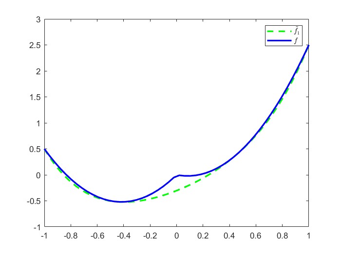
Then we compute $f^{(\mathbf{k})}(x)\coloneqq\mathbb{E}_{\mu}[p^{(\mathbf{k})}(x,\xi)]$ for each above $\mathbf{k}$ and plot them with the true expected recourse function $f(x)=\mathbb{E}_{\mu}[f_{2}(x,\xi)]$ in Figure 2. Specifically, the function $f^{(1,2,2)}$ is plotted in the dashed line, the function $f^{(1,3,2)}$ is plotted in the dotted line, the function $f^{(2,2,2)}$ is plotted in the dash-dotted line, the function $f^{(2,3,3)}$ is plotted in the plus sign line, and the expected recourse $f$ is plotted in the solid line. In addition, we plot global minimizers of all these $f^{(\mathbf{k})}(x)$ on $X$ in blue dots.

Figure 2: Compute $\mathbb{E}_{\mu}[p^{(\mathbf{k})}(x,\xi)]$ and $\mathbb{E}[f_{2}(x,\xi)]$ for Example 4.3, where dashed line is $f^{(1,2,2)}$, dotted line is $f^{(1,3,2)}$, dash-dotted line is $f^{(2,2,2)}$, plus sign line is $f^{(2,3,3)}$, solid line is $f$, and big dots are minimizers.

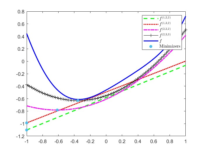
Clearly, the global minimum of $\mathbb{E}_{\mu}[p^{(\mathbf{k})}(x,\xi)]$ on $X$ increases as the relaxation order increases. Denote by $f_{min}^{(\mathbf{k})}$ and $x^{\mathbf{(k)}}$ the global minimum and minimizer of (3.1). We report the computational results in the following table.

$$\begin{array}[]{|c|c|c|c|c|}\hline\cr\mathbf{k}&(1,2,2)&(1,3,2)&(2,2,2)&(2,3,3)\\ \hline\cr f_{min}^{(\mathbf{k})}&-1.1018&-0.9883&-0.7821&-0.6296\\ \hline\cr x^{(\mathbf{k})}&-1.0000&-1.0000&-0.6149&-0.3555\\ \hline\cr\end{array}$$

From Figure 2, one can observe that when $\mathbf{k}=(2,3,3)$, $x^{(\mathbf{k})}=-0.3555$ is close to the global optimizer of the two-stage SP. By sample average approximations, we compute

$$f(-0.3555)\,\approx\,\frac{1}{100}\sum\limits_{i=1}^{100}f_{2}(-0.3555,\,0.01\cdot i)=-0.6042,$$

which is close to $f^{(\mathbf{k})}(-0.3555)=-0.6296$. One can further improve the approximation quality by increasing the relaxation order.

4.2 Relaxations of problem (2.6)

For easy of reference, we repeat the optimization problem (2.6) below:

$$\left\{\begin{array}[]{cl}\max\limits_{p_{i}\in\mathbb{R}[x]}&\int_{\mathcal{F}_{i}}p_{i}(x){\tt d}\nu_{i}\\ \mbox{s.t.}&F(x,y,\xi^{(i)})-p_{i}(x)\in\mathscr{P}(K_{i})^{x,y},\end{array}\right.$$

where $\nu_{i}$ is a given probability measure supported on $\mathcal{F}_{i}$, and $K_{i}$ is a semialgebraic set determined by

$$g_{1}(x)\geq 0,\quad g_{2}(x,y,\xi^{(i)})\geq 0.$$ (4.8)

The functions $g_{1},g_{2}(\bullet,\xi^{(i)})$ can be viewed as polynomial tuples in $(x,y)$. Denote the quadratic module

$$\mathit{QM}[g_{1},g_{2}(\bullet,\xi^{(i)})]^{x,y}\,\coloneqq\,\mathit{QM}[g_{1}]^{x,y}+\mathit{QM}[g_{2}(\bullet,\xi^{(i)})]^{x,y}$$

as a subset in $\mathbb{R}[x,y]$, where

$$\mathit{QM}[g_{1}]^{x,y}\,\coloneqq\,\sum\limits_{i\in\mathcal{I}_{1}}g_{1,i}(x)\cdot\Sigma[x,y],\quad\mathit{QM}[g_{2}(\bullet,\xi^{(i)})]^{x,y}\,\coloneqq\,\sum\limits_{j\in\mathcal{I}_{2}}g_{2,j}(x,y,\xi^{(i)})\cdot\Sigma[x,y].$$

Let $k\geq\max\{\lceil\deg(F)/2\rceil,\lceil d_{1}/2\rceil\}$. The $k$th order SOS relaxation of (2.6) is

$$\left\{\begin{array}[]{cl}\max\limits_{p_{i}\in\mathbb{R}[x]}&\int_{\mathcal{F}_{i}}p_{i}(x){\tt d}{\nu_{i}}\\ \mbox{s.t.}&F(x,y,\xi^{(i)})-p_{i}(x)\in\mathit{QM}[g_{1},g_{2}(\bullet,\xi^{(i)})]_{2k}^{x,y},\end{array}\right.$$ (4.9)

where $\mathit{QM}[g_{1},g_{2}(\bullet,\xi^{(i)})]_{2k}^{x,y}$ denotes the $k$th order truncation of $\mathit{QM}[g_{1},g_{2}(\bullet,\xi^{(i)})]^{x,y}$.

Theorem 4.4.

Suppose $\mathit{QM}[g_{1},g_{2}(\bullet,\xi^{(i)})]^{x,y}$ is archimedean and $f_{2}(x,\xi^{(i)})$ is continuous on $\mathcal{F}_{i}$. For a given measure $\nu_{i}$, problem (4.9) is solvable with an optimal solution $p_{i}^{(k)}(x)$ when $k$ is large enough, and

$$\int_{\mathcal{F}_{i}}|f_{2}(x,\xi^{(i)})-p_{i}^{(k)}(x)|{\tt d}{\nu_{i}}\rightarrow 0\quad\mbox{as}\quad k\rightarrow\infty.$$

Proof.

Under the archimedean condition, $K_{i}$ in (4.8) is compact, thus $\mathcal{F}_{i}$ is compact. Assume $f_{2}(x,\xi^{(i)})$ is continuous on $\mathcal{F}_{i}$. By Theorem 2.4, for every $\varepsilon>0$, there exists a polynomial $p_{i}(x)$ that is feasible for (2.6) and satisfies $\int_{\mathcal{F}_{i}}|f_{2}(x,\xi^{(i)})-p_{i}(x)|{\tt d}{\nu_{i}}\leq\varepsilon$; that is,

$$F(x,y,\xi^{(i)})-(p_{i}(x)-\varepsilon)\,\geq\,\varepsilon\,>\,0,\quad\forall(x,y)\in K_{i}.$$

By Putinar’s Positivstellensatz, $F(x,y,\xi^{(i)})-(p_{i}(x)-\varepsilon)\in\mathit{QM}[g_{1},g_{2}(\bullet,\xi^{(i)})]^{x,y}$. So there exists $k_{\varepsilon}\in\mathbb{N}$ that is sufficiently large such that the polynomial $p_{i}(x)-\varepsilon$ is feasible for (4.9) at the $k_{\varepsilon}$th relaxation. At the $k_{\varepsilon}$th relaxation, (4.9) is bounded from above and has a nonempty closed feasible set, so it is solvable with an optimizer $p_{i}^{(k_{\varepsilon})}(x)$. Then we have

$$\int_{\mathcal{F}_{i}}|f_{2}(x,\xi^{(i)})-p_{i}^{(k_{\varepsilon})}(x)|{\tt d}\nu_{i}\,\leq\,\int_{\mathcal{F}_{i}}|f_{2}(x,\xi^{(i)})-(p_{i}(x)-\varepsilon)|{\tt d}{\nu_{i}}\,\leq\,2\varepsilon.$$

Since $\mathit{QM}[g_{1},g_{2}(\bullet,\xi^{(i)})]^{x,y}_{2k}\subseteq\mathit{QM}[g_{1},g_{2}(\bullet,\xi^{(i)})]^{x,y}_{2k+2}$ for every $k$, the optimal value of (4.9) increases monotonically as the relaxation order grows. In other words, $k_{\varepsilon}\rightarrow\infty$ as $\varepsilon\rightarrow 0$. So the conclusion holds. ∎

Example 4.5.

Consider the two-stage SP as in (1.1) with $x,\xi\in\mathbb{R}$, $f_{1}(x)=0$, $y\in\mathbb{R}^{2}$ and

$$S=\{\xi^{(1)},\xi^{(2)}\}=\{-0.1,0.2\},\quad X=\{x\in\mathbb{R}:x(1-x)\geq 0\}.$$

The second-stage optimization problem is given as

$$\left\{\begin{array}[]{rl}f_{2}(x,\xi)=\min\limits_{y\in\mathbb{R}^{2}}&x^{2}y_{1}+\xi xy_{2}\\ \mbox{s.t.}&y_{1}-\xi\geq 0,\,y_{2}\geq 0,\\ &x-y_{1}-y_{2}\geq 0.\end{array}\right.$$ (4.10)

Clearly, $\mathcal{F}_{1}=X=[0,1]$ and $\mathcal{F}_{2}=[0.2,1]$. Since the second-stage optimization problem is linear in $y$, we can analytically solve the recourse function at each realization as

$$f_{2}(x,\xi^{(1)})\,=\,-0.2x^{2}-0.01x,\quad f_{2}(x,\xi^{(2)})\,=\,0.2x^{2}.$$

Select $\nu_{1},\nu_{2}$ as uniform probability measures supported on $\mathcal{F}_{1},\mathcal{F}_{2}$, respectively. We solve (4.9) with initial relaxation order $k=2$. The computed lower approximating functions are

$$\begin{array}[]{l}p_{1}^{(2)}(x)\,=\,-0.0004-0.0066x-0.2112x^{2}+0.0150x^{3}-0.0069x^{4},\\ p_{2}^{(2)}(x)\,=\,-0.0004+0.0028x+0.1926x^{2}+0.0084x^{3}-0.0034x^{4}.\end{array}$$

They provide reasonably good approximations of the true recourse function. In fact, we have

$$\sup_{x\in X}|f_{2}(x,\xi^{(1)})-p_{1}^{(1)}(x)|\leq 4\cdot 10^{-4},\quad\sup_{x\in X}|f_{2}(x,\xi^{(2)})-p_{2}^{(2)}(x)|\leq 7\cdot 10^{-5}.$$

Therefore, for an arbitrary probability measure $\mu=\lambda_{1}\delta_{-0.1}+(1-\lambda_{2})\delta_{0.2}$ with $\lambda\in[0,1]$, the recourse approximation $\tilde{f}(x)\coloneqq\lambda_{1}\cdot p_{1}^{(2)}(x)+(1-\lambda)\cdot p_{2}^{(2)}(x)$ satisfies

$$\sup_{x\in X}|f(x)-\tilde{f}(x)|\leq 4\cdot 10^{-4}.$$

4.3 Solving the first-stage problem

In this subsection, we discuss how to replace the recourse function $f_{2}(x,\xi)$ by the approximating polynomial function $p(x,\xi)$ in the two-stage SP (1.1), and solve the first-stage problem to global optimality. Let $p(x,\xi)$ be a selected polynomial lower approximating function of $f_{2}(x,\xi)$. The two-stage SP (1.1) can be approximated by the polynomial optimization problem in (3.1), which takes the form of

$$\left\{\begin{array}[]{cl}\min\limits_{x\in\mathbb{R}^{n_{1}}}&\tilde{f}(x)\coloneqq f_{1}(x)+\mathbb{E}_{\mu}[p(x,\xi)]\\ \mbox{s.t.}&g_{1}(x)\geq 0,\end{array}\right.$$

where $g_{1}(x)=(g_{1,i}(x))_{i\in\mathcal{I}_{1}}$ is the polynomial tuple given as in (4.1). The above problem can be solved globally by Moment-SOS relaxations. Denote

$$d_{3}\,\coloneqq\,\max\big{\{}\deg\big{(}\tilde{f}\big{)},\quad\deg(g_{1})\big{\}}.$$ (4.11)

For $k\in\mathbb{N}$ such that $2k\geq d_{3}$, the $k$th order SOS relaxation of (3.1) is

$$\left\{\begin{array}[]{cl}\max\limits_{\gamma\in\mathbb{R}}&\gamma\\ \mbox{s.t.}&\tilde{f}(x)-\gamma\in\mathit{QM}[g_{1}]_{2k}^{x},\end{array}\right.$$ (4.12)

where $\mathit{QM}[g]_{2k}^{x}$ denotes the $k$th order truncation of

$$\mathit{QM}[g_{1}]^{x}\,\coloneqq\,\sum\limits_{i\in\mathcal{I}_{1}}g_{1,i}(x)\cdot\Sigma[x].$$

The dual problem of (4.12) is the $k$th order moment relaxation of (3.1), which is

$$\left\{\begin{array}[]{cl}\min\limits_{z\in\mathbb{R}^{\mathbb{N}_{2k}^{n_{1}}}}&\langle\tilde{f},z\rangle\\ \mbox{s.t.}&z_{0}=1,\,M_{k}[z]\succeq 0,\\[3.61371pt] &L_{g_{1,i}}^{(k)}[z]\succeq 0\,(i\in\mathcal{I}_{1}).\end{array}\right.$$ (4.13)

In the above, $M_{k}[z]$ and each $L_{g_{i,i}}^{(k)}[z]$ are moment and localizing matrices defined as in (1.11). For each $k$, the optimization problems (4.12)–(4.13) are semidefinite programming problems. Suppose $\tilde{f}_{0}$ is the optimal value of (3.1) and $\tilde{f}_{k}$ is the optimal value of (4.13) at $k$th relaxation order. Under the archimedean condition of $\mathit{QM}[g_{1}]^{x}$, the dual pair (4.12)–(4.13) has the asymptotic convergence (see [20])

$$\tilde{f}_{k}\leq\tilde{f}_{k+1}\leq\cdots\leq\tilde{f}_{0}\quad\mbox{and}\quad\lim_{k\to\infty}\tilde{f}_{k}=\tilde{f}_{0}.$$

Interestingly, the finite convergence, i.e., $\tilde{f}_{k}=\tilde{f}_{0}$ for $k$ large enough, holds when $\tilde{f},g_{1}$ are given by generic polynomials. It can be verified by a convenient rank condition called flat truncation [30]. Suppose $z^{*}$ is an optimizer of (4.13) at the $k$th relaxation. If there exists $t\in[d_{3},k]$ such that

$$\mbox{rank}\,M_{t-d_{3}}[z^{*}]\,=\,\mbox{rank}\,M_{t}[z^{*}],$$

then (4.13) is a tight relaxation of (3.1). In this case, problem (3.1) has $\mbox{rank}\,M_{t}[z^{*}]$ number of global optimal solutions. These optimal solutions can be extracted via Schur decompositions [15]. We refer to [21, 30, 31] for detailed study of polynomial optimization.

5 Numerical Experiments

In this section, we demonstrate the effectiveness of our method through numerical experiments. The computations were carried out in MATLAB R2023a on a laptop equipped with an 8th Generation Intel®Core™i7-12800H CPU and 32 GB RAM. The computations were implemented with the MATLAB software Yalmip [26], Mosek [29] GloptiPoly 3 [13], and SeDuMi [42]. For clarity, computational results are reported to four decimal places.

In Algorithms 3.1 and 3.3, all optimization problems are solved using Moment-SOS relaxations. For the linear conic optimization problem (1.7), we choose a specific relaxation order $\mathbf{k}=(k_{1},k_{2},k)$ to compute the lower approximating function $p(x,\xi)$ from problem (4.7). For the optimization problem (2.4), we select a prescribed relaxation order $k$ to determine the the lower approximating function $p_{i}(x)$ from (4.9). The polynomial optimization problem (3.1) is globally solved using a hierarchy of semidefinite relaxations, as detailed in (4.13).

For the sake of simplicity, we denote the computed lower approximating function for $f(x)$ at the $t$th iteration as $\tilde{f}_{t}(x)$, with $\tilde{f}_{t}$ and $\tilde{x}^{(t)}$ representing the global optimal value and the solution obtained from (3.1) in the corresponding iteration. We use diff to denote the gap between the upper and lower bounds (i.e., $v^{+}-v^{-}$) at each iteration.

First, we consider a synthetic example where the recourse function has an explicit analytical expression.

Example 5.1.

Consider the two-stage SP

$$\left\{\begin{array}[]{cl}\min\limits_{x\in\mathbb{R}^{2}}&2x_{1}x_{2}^{2}-x_{1}^{2}+\mathbb{E}_{\mu}[f_{2}(x,\xi)]\\ \mbox{s.t.}&1-x_{1}^{2}-x_{2}^{2}\geq 0,\end{array}\right.$$ (5.1)

where $\xi\in\mathbb{R}$ is univariate and $f_{2}(x,\xi)$ is the optimal value function of the problem

$$\left\{\begin{array}[]{cl}\min\limits_{y\in\mathbb{R}}&x_{2}y\\ \mbox{s.t.}&x_{1}-2\xi\leq y\leq x_{1}+\xi.\end{array}\right.$$

Since the second-stage problem is linear in $y$ with box constraints, one can obtain the following analytical expression of the recourse function:

$$f_{2}(x,\xi)=\left\{\begin{array}[]{ll}x_{2}(x_{1}-2\xi)&\mbox{if $x_{2}\geq 0$},\\[3.61371pt] x_{2}(x_{1}+\xi)&\mbox{if $x_{2}\leq 0$}.\end{array}\right.$$

Clearly, $f_{2}(x,\xi)$ is continuous but nonconvex, and is not a polynomial. Assume $\mu$ is a probability measure with the support $S=[0,1]$, moments $\mathbb{E}_{\mu}[\xi]=0.6$ and $\mathbb{E}_{\mu}[\xi^{2}]=0.5$. Then we can find an explicit expression of the overall objective function

$$f(x)=2x_{1}x_{2}^{2}-x_{1}^{2}+\mathbb{E}_{\mu}[f_{2}(x,\xi)]=\left\{\begin{array}[]{ll}2x_{1}x_{2}^{2}-x_{1}^{2}+x_{1}x_{2}-1.2x_{2}&\mbox{if $x_{2}\geq 0$},\\[3.61371pt] 2x_{1}x_{2}^{2}-x_{1}^{2}+x_{1}x_{2}+0.6x_{2}&\mbox{if $x_{2}\leq 0$}.\end{array}\right.$$

One can get the following global optimal solution and the optimal value of (5.1) by solving two polynomial optimization problems with Moment-SOS relaxations:

$$x^{*}=(-0.6451,0.7641)^{T},\quad f^{*}=-2.5793.$$

Now we apply Algorithm 3.1 to solve this problem, and compare our results with the above true solution. Clearly, $\mathcal{F}=X\times S$. Select $\alpha=0.1$, $\epsilon=0.001$, and let $\nu$ be the uniform probability measure supported on $\mathcal{F}$. For the relaxation order $\mathbf{k}=(2,2,2)$, Algorithm 3.1 terminates at the initial loop $t=1$ with the computed objective approximation

$$\tilde{f}_{1}(x)\,=\,2x_{1}x_{2}^{2}-x_{1}^{2}+(-0.6171x_{2}^{2}+x_{1}x_{2}-0.3000x_{2}-0.3281).$$

By solving optimization problem (3.1), we obtain the following candidate solution and the corresponding lower bound for the optimal objective value

$$\tilde{x}^{*}=(-0.6417,0.7670)^{T},\quad\tilde{f}^{*}=-2.5801.$$

Since $f^{*}=-2.5792$, the gap ${\tt diff}=\tilde{f}^{*}-\tilde{f}^{*}=8.8310\cdot 10^{-4}<0.001$. Compared to the true optimizer and the optimal value, the computed polynomial lower approximating function, even with a low degree, provides a good approximation.

In the next example, we show that by increasing the relaxation order, one can improve the approximation quality of the polynomial lower approximating functions.

Example 5.2.

Consider the two-stage SP as in (1.1) with $x,\xi\in\mathbb{R}$, $f_{1}(x)=0$, $y\in\mathbb{R}^{2}$, $\mu\sim\mathcal{U}(S)$ and

$$X=\{x\in\mathbb{R}:1-x^{2}\geq 0\},\quad S=\{\xi\in\mathbb{R}:\xi(1-\xi)\geq 0\},$$

where $\mu\in\mathcal{U}(S)$ denotes the uniform probability measure. The second-stage problem is given by

$$\left\{\begin{array}[]{rl}f_{2}(x,\xi)=\min\limits_{y\in\mathbb{R}^{2}}&xy_{1}+2xy_{2}\\ \mbox{s.t.}&y_{1}-x-\xi\geq 0,\\ &y_{2}-x+\xi\geq 0,\\ &2x+3\xi-y_{1}-y_{2}\geq 0.\end{array}\right.$$

Clearly, the second-stage optimization problem is feasible for every $x\in X$ and $\xi\in S$, so we have $\mathcal{F}=X\times S$. Select $\alpha=0.1$, $\epsilon=0.1$, and let $\nu$ be the uniform probability measure supported on $\mathcal{F}$. Apply Algorithm 3.1 to this problem. We consider two different relaxation orders $\mbox{(i)}\,\mathbf{k}=(2,4,3)$; $\mbox{(ii)}\,\mathbf{k}=(4,4,4)$.

(i) When $\mathbf{k}=(2,4,3)$, Algorithm 3.1 terminates at the loop $t=4$. We record the computed polynomial objective approximations in each loop below:

$$\begin{array}[]{ll}\tilde{f}_{1}(x)=-0.4330+1.0000x+1.7010x^{2},&\tilde{f}_{2}(x)=-0.2500+1.0000x+0.7498x^{2},\\ \tilde{f}_{3}(x)=-0.4330+1.0000x+1.7009x^{2},&\tilde{f}_{4}(x)=-0.2586+1.0000x+0.8248x^{2}.\end{array}$$

The computed solutions and lower/upper bounds for the optimal values at each iteration are listed in Table 1.

$t$	$1$	$2$	$3$	$4$
$\tilde{x}^{(t)}$	$-0.2939$	$-0.6668$	$-0.2939$	$-0.6062$
$\tilde{f}_{t}(\tilde{x}^{(t)})$	$-0.5800$	$-0.5834$	$-0.5800$	$-0.5617$
$f(\tilde{x}^{(t)})$	$-0.4756$	$-0.3331$	$-0.4756$	$-0.4131$
$\tt diff$	$0.1044$	$0.1044$	$0.1044$	$0.0861$

Table 1: Computational results with $\mathbf{k}=(2,4,3)$ for Example 4.5

To evaluate $f(\tilde{x}^{(t)})$, we solve the second-stage optimization problem by Moment-SOS relaxations and use the sample average of $\{f_{2}(\bullet,0.01\cdot i)\}_{i\in[100]}$. The output solution and the best lower bound of the optimal value are

$$\tilde{x}^{*}\,=\,\tilde{x}^{(1)}\,=\,-0.2939,\quad\tilde{f}^{*}\,=\,\tilde{f}_{4}(\tilde{x}^{(4)})\,=\,-0.5617.$$

(ii) When $\mathbf{k}=(4,4,4)$, Algorithm 3.1 terminates at the initial loop $t=1$ with the polynomial objective approximation

$$\tilde{f}_{1}(x)\,=\,-0.3035+1.0000x+1.0034x^{2}+0.7999x^{4}.$$

By solving optimization problem (3.1), we get the solution and the lower bound of the optimal value

$$\tilde{x}^{*}=\tilde{x}^{(1)}\,=\,-0.3979,\quad\tilde{f}^{*}=\tilde{f}_{1}(\tilde{x}^{(1)})\,=\,-0.5225.$$

We again evaluate $f(\tilde{x}^{*})$ by the sample average of $\{f_{2}(\bullet,0.01\cdot i)\}_{i\in[100]}$ and obtain

$$f(\tilde{x}^{*})=-0.5198,\quad{\tt diff}=f(\tilde{x}^{(1)})-\tilde{f}_{1}(\tilde{x}^{(1)})=0.0027<0.1.$$

Compared to the previous case, it is clear that the increase of the relaxation order leads to a better polynomial approximation and a smaller gap between the upper and lower bounds of objective values.

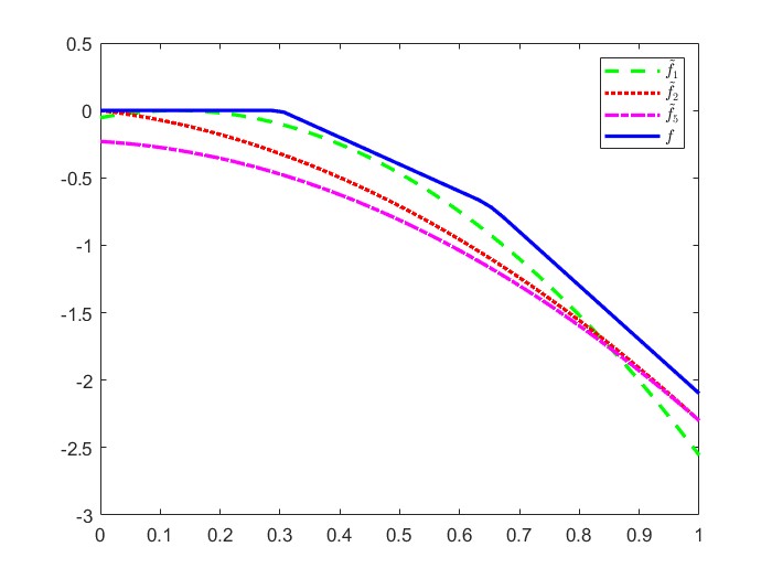
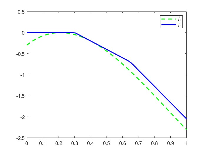
In addition, we plot the expected recourse function $f$ (evaluated via sample averages) and computed polynomial lower bound functions in Figure 3. The left subfigure is for the case $\mathbf{k}=(2,4,3)$, and the right subfigure is for the case $\mathbf{k}=(4,4,4)$. In both subfigures, $f$ is plotted with solid lines and $\tilde{f}_{1}$ is plotted with dashed lines. In the left panel, $\tilde{f}_{2}$ is plotted with the dotted line, $\tilde{f}_{4}$ is plotted with the dash-dotted line.

Figure 3: The recourse function and its approximations for Example 5.2. The left panel is for $\mathbf{k}=(2,4,3)$, and the right panel is for $\mathbf{k}=(4,4,4)$. The dashed line is for $\tilde{f}_{1}$, dotted line is for $\tilde{f}_{2}$, dash-dotted line is for $\tilde{f}_{4}$ and the solid line is for $f$.

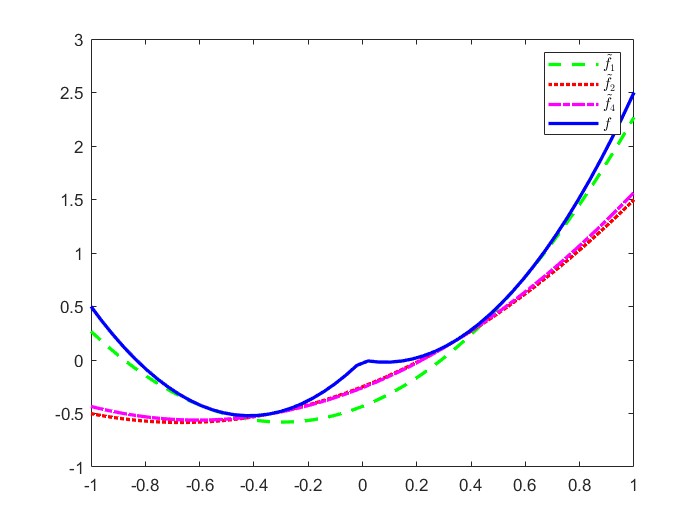
It can be observed that the polynomial approximation with order $\mathbf{k}=(4,4,4)$ also gives a better approximation to the true optimizer compared to the case $\mathbf{k}=(2,4,3)$. On the other hand, a small increase of the relaxation order can heavily enlarge the dimension of the corresponding linear conic optimization problem (4.4). For the case $\mathbf{k}=(2,4,3)$, there are $210$ scalar variables, $7$ matrix variables equivalent to $1350$ scalar variables when scalarized, and $1365$ constraints. In contrast, for the case where $\mathbf{k}=(4,4,4)$, there are $495$ scalar variables, $7$ matrix variables which scalarize to $6265$ variables, and $6290$ constraints.

Next we apply Algorithm 3.1 to a problem of a larger scale, where the second-stage variable $y\in\mathbb{R}^{10}$. In this example, the polynomial lower approximating functions again yield a high-quality solution with relatively low degrees.

Example 5.3.

Consider the two-stage SP

$$\left\{\begin{array}[]{cl}\min\limits_{x\in\mathbb{R}^{2}}&x_{1}x_{2}+\mathbb{E}_{\mu}[f_{2}(x,\xi)]\\ \mbox{s.t.}&1-x_{1}^{2}-x_{2}^{2}\geq 0,\end{array}\right.$$

where $\xi\in S=[0,1]$ follows a uniform distribution on $S$, and $f_{2}(x,\xi)$ is the optimal value function of the problem (here $e=(1,\ldots,1)^{T}\in\mathbb{R}^{n_{2}}$ is the vector of all ones)

$$\left\{\begin{array}[]{cl}\min\limits_{y\in\mathbb{R}^{10}}&\|y\|^{2}-y_{1}^{2}-\xi\cdot e^{T}y\\ \mbox{s.t.}&(x_{2}+2)y_{1}-x_{1}+2\xi\geq 0,\\ &2+x_{2}+(x_{1}-2)y_{2}\geq 0,\\ &10-x_{1}-e^{T}y\geq 0,\\ &y_{i}\geq 0,\,i=2,\ldots,9.\end{array}\right.$$

Then $\mathcal{F}=X\times S$ since the second-stage problem is feasible for every $x\in X$ and $\xi\in S$. Now we apply Algorithm 3.1 to this problem. We select $\alpha=0.1$, $\epsilon=0.06$, and let $\nu$ be the uniform probability measure supported on $\mathcal{F}$. Denote by $\tilde{p}_{t}(x)$ the computed lower bound function for $f_{2}(x,\xi)$ at the $t$th loop. For the degree bound $\mathbf{k}=(2,2,2)$, we obtain polynomial objective approximations

$$\begin{array}[]{l}\tilde{f}_{1}(x)\,=\,x_{1}x_{2}+(-5.0868+0.4978x_{1}-0.0023x_{2}-0.0069x_{1}^{2}-0.0113x_{2}^{2}),\\[3.61371pt] \tilde{f}_{2}(x)\,=\,x_{1}x_{2}+(-5.0894+0.4730x_{1}+0.0310x_{2}-0.0192x_{1}^{2}-0.0434x_{1}x_{2}-0.0477x_{2}^{2}).\end{array}$$

By solving optimization problem (3.1), we get optimal solutions for each approximation and corresponding lower/upper bounds for the optimal value:

$$\begin{array}[]{lll}\tilde{x}^{(1)}\,=\,(-0.8033,0.5956)^{T},&\tilde{f}_{1}(\tilde{x}^{(1)})\,=\,-5.9750,&f(\tilde{x}^{(1)})\,=\,-5.8801,\\ \tilde{x}^{(2)}\,=\,(-0.8037,0.5950)^{T},&\tilde{f}_{2}(\tilde{x}^{(2)})\,=\,-5.9379,&f(\tilde{x}^{(2)})\,=\,-5.8801.\end{array}$$

In the above, each $f(\tilde{x}^{(t)})$ is approximated by the sample average of $\{f_{2}(\bullet,0.01\cdot i)\}_{i\in[100]}$. Since

$${\tt diff}\,=\,f(\tilde{x}^{(2)})-\tilde{f}_{2}(\tilde{x}^{(2)})\,=\,0.0578\,<\,0.06,$$

we have that Algorithm 3.1 terminates at the loop $t=2$.

Our last test example is a joint shipment planning and pricing problem, which can be modeled in the form of two-stage SP [24].

Example 5.4.

Consider one product in a network consisting with $M$ factory and $N$ retailer stores. For each $i\in[M]$, factory $i$ has an initial schedule to produce the product with amount $x_{i}$ at cost $c_{1i}$ per unit, and it may allow additional production with amount $y_{i}$ at cost $c_{2i}>c_{1i}$ per unit. In addition, to ship a unit of item from factory $i$ to store $j$ cost $s_{ij}$. Let $x_{0}$ denote the product price and $z_{ij}$ denote the product amount shipped from factory $i$ to store $j$. The goal is to fulfill the demand with the lowest cost. Suppose the demand is linearly dependent on the price $x_{0}$ and some random vectors $\xi=(\xi_{1},\ldots,\xi_{n_{0}})$. In addition, suppose there exist highest price and production limits. That is, there are scalars $d_{0},d_{1,i},d_{2,i}>0$ such that $x_{0}\leq c_{0,0}$ and $x_{i}\leq c_{0,i},\,y_{i}\leq c_{0,i}$ for every $i\in[M]$. Let

$$c_{j}=(c_{j,1},\ldots,c_{j,M})^{T},\quad d_{j}=(d_{j,1},\ldots,d_{j,M})^{T},\quad j=1,2.$$

The shipment planning problem can be formulated as

$$\left\{\begin{array}[]{cl}\min\limits_{x_{0}\in\mathbb{R}}&\mathbb{E}_{\mu}[f_{2}(x_{0},x,\xi)]\\ \mbox{s.t.}&d_{0}\geq x_{0}\geq 0,\end{array}\right.$$

where $f_{2}(x_{0},x,\xi)$ is the optimal value of

$$\left\{\begin{array}[]{cl}\min\limits_{(x,y,z)}&c_{1}^{T}x+c_{2}^{T}y+\sum\limits_{i=1}^{M}\sum\limits_{j=1}^{N}(s_{ij}-x_{0})z_{ij}\\[3.61371pt] \mbox{s.t.}&a_{j}(\xi)x_{0}+b_{j}(\xi)-\sum\limits_{i=1}^{M}z_{ij}\geq 0,\,\forall j\in[N],\\[3.61371pt] &x_{i}+y_{j}-\sum\limits_{j=1}^{N}z_{ij}\geq 0,\,\forall i\in[M],\\[3.61371pt] &d_{1}\geq x\geq 0,\,x=(x_{1},\ldots,x_{M})\in\mathbb{R}^{M}\\[3.61371pt] &d_{2}\geq y\geq 0,\,y=(y_{1},\ldots,y_{M})\in\mathbb{R}^{M},\\[3.61371pt] &z\geq 0,\,z=(z_{ij})_{i\in[M],j\in[N]}\in\mathbb{R}^{M\times N}.\end{array}\right.$$

Up to a proper scaling, suppose the parameters are selected as

$$\begin{array}[]{lllllll}\hline\cr M=2,&N=3,&d_{0}=1,&d_{1,1}=1,&d_{1,2}=1,&d_{2,1}=1\\ d_{2,2}=1&c_{1,1}=0.2,&c_{1,2}=0.2,&c_{2,1}=0.44,&c_{2,2}=0.46,&s_{1,1}=0.1,\\ s_{1,2}=0.2,&s_{1,3}=0.3,&s_{2,1}=0.3,&s_{2,2}=0.2,&s_{2,3}=0.1.\\ \hline\cr\end{array}$$

(i) Consider $\xi=(\xi_{1},\xi_{2})$ whose probability measure $\mu$ follows the truncated standard normal distribution supported on $S=[0,1]^{2}$. We set

$$\begin{array}[]{lll}\hline\cr a_{1}(\xi)\,=\,-2\xi_{1},&a_{2}(\xi)\,=\,-2.5(\xi_{1}+0.01),&a_{3}(\xi)\,=\,-3\xi_{1}-0.06,\\ b_{1}(\xi)\,=\,0.5\xi_{2}+3,&b_{2}(\xi)\,=\,0.7\xi_{2}+4,&b_{3}(\xi)\,=\,-0.1\xi_{2}+5.\\ \hline\cr\end{array}$$

Now we apply Algorithm 3.1 to this problem. We generate $N=500$ independent samples following the distribution $\mu$. Select $\alpha=0.1$, $\epsilon=0.3$ and let $\nu$ be the Cartesian product of $\mu$ and the uniform probability measure supported on $X$. For the relaxation order $\mathbf{k}=(2,2,2)$, Algorithm 3.1 terminates at the loop $t=3$. To improve the approximation, we execute two more iterations, and obtain the following objective approximations:

$$\begin{array}[]{ll}\tilde{f}_{1}(x_{0})\,=\,-0.05386+0.8499x_{0}-3.3528x_{0}^{2},&\tilde{f}_{2}(x_{0})\,=\,-0.5393x_{0}-1.7613x_{0}^{2},\\ \tilde{f}_{3}(x_{0})\,=\,-0.5943x_{0}-1.7057x_{0}^{2},&\tilde{f}_{4}(x_{0})\,=\,-0.0019-0.5958x_{0}-1.7023x_{0}^{2}\\ \tilde{f}_{5}(x_{0})\,=\,-0.2300-0.2653x_{0}-1.8046x_{0}^{2}.\end{array}$$

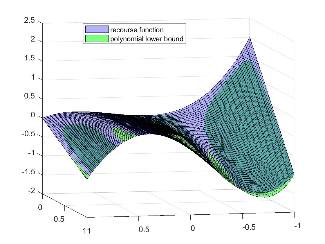
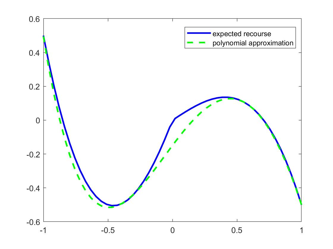
We report the computational results in Table 2 and plot the expected recourse function and its approximations in the left subgraph of Figure 4. In the figure, $f$ is plotted in the solid line, $\tilde{f}_{1}$ is plotted in the dashed line, $\tilde{f}_{2}$ is plotted in the dotted line and $\tilde{f}_{5}$ is plotted in the dash-dotted line.

$t$	$1$	$2$	$3$	$4$	$5$
$\tilde{x}_{0}^{(t)}$	$1.0000$	$1.0000$	$1.0000$	$1.0000$	$1.0000$
$\tilde{f}_{t}(\tilde{x}_{0}^{(t)})$	$-2.5568$	$-2.3005$	$-2.3000$	$-2.3000$	$-2.2999$
$f(\tilde{x}_{0}^{(t)})$	$-2.1000$	$-2.1000$	$-2.1000$	$-2.1000$	$-2.1000$
${\tt diff}$	$0.4580$	$0.2018$	$0.2012$	$0.2012$	$0.2011$

Table 2: Computational results with $\mathbf{k}=(2,2,2)$ for Example 5.4

(ii) Consider the situation that $a_{j}(\xi)$ and $b_{j}(\xi)$ have the following finite realizations with equal probabilities:

$$\begin{array}[]{lll}\hline\cr a_{1}(\xi)\in\{-0.5,-2\}&a_{2}(\xi)\in\{-3\}&a_{3}(\xi)\in\{-1,-3\}\\ b_{1}(\xi)\in\{3\},&b_{2}(\xi)\in\{4,7\},&b_{3}(\xi)\in\{5\}\\ \hline\cr\end{array}$$

We apply Algorithm 3.3 to this problem. Select $\alpha=0.1$, $\epsilon=0.3$ and let each $\nu_{i}$ be the uniform probability measure supported on $X$. For the relaxation order $k=4$, Algorithm 3.3 terminates at the loop $t=2$ with the following objective approximations:

$$\begin{array}[]{l}\tilde{f}_{1}(x_{0})\,=\,-0.2981+2.9749x_{0}-8.0524x_{0}^{2}+3.0694x_{0}^{3},\\ \tilde{f}_{2}(x_{0})\,=\,-0.3001+2.9921x_{0}-8.0952x_{0}^{2}+3.1002x_{0}^{3}.\end{array}$$

The output solution and the corresponding bounds for the optimal value are

$$\tilde{x}_{0}^{*}=1.0000,\quad\tilde{f}^{*}=-2.3030,\quad f(\tilde{x}^{*})=-2.0500.$$

The gap ${\tt diff}=f(\tilde{x}^{*})-\tilde{f}^{*}=0.2530<0.3$. We plot the expected recourse function and its polynomial approximation in right subgraph of Figure 4. In the figure, $f$ is plotted in the solid line, $\tilde{f}_{1}$ is plotted in the dashed line.

Figure 4: The recourse function and its approximations for Example 5.4. The left is for case (i) and the right is for case (ii). In both subgraphs, the dashed line is for $\tilde{f}_{1}$ and and the solid line is for $f$. Particularly in the left, dotted line is for $\tilde{f}_{2}$ and dash-dotted line is for $\tilde{f}_{5}$.

It is clear that our polynomial approximating bound functions provide good approximations to the true objective function.

6 Conclusions

In this paper, we have explored a novel computational method for computing global optimal solutions of two-stage stochastic programs through polynomial optimization. Our proposed method hinges on the computation of the polynomial lower bound of the recourse function. These lower bound functions can be determined by the solutions of a sequence of linear conic optimization problems, where the size of the decision variable does not depend on the number of scenarios in the second stage problem. The approach presents significant computational advantages. It can identify a tight lower bound for the global optimal value of (1.1), which can be used to certify the global optimality of a candidate solution obtained by other methods. Furthermore, our method is notably effective when the random variables follow empirical distributions with a large number of scenarios or continuous distributions. In the future, we plan to further explore the structure of the two-stage stochastic problems so that our proposed approach can be used to solve large-scale problems more efficiently. We also aim to improve the efficiency of polynomial lower approximating functions, particularly for those with low degrees.

Acknowledgement. The project was partially done when the authors attended the SQuaRE program hosted by the American Institute for Mathematics (AIM). The authors thank AIM for providing a supportive and collaborative environment.

References

- [1] J. R. Birge and F. Louveaux, Introduction to Stochastic Programming, Springer, New York, 2011.
- [2] P. Borges, C. Sagastizábal and M. Solodov, A regularized smoothing method for fully parameterized convex problems with applications to convex and nonconvex two-stage stochastic programming, Math. Program., 189 (2021), pp. 117–149.
- [3] F. H. Clarke, Optimization and Nonsmooth Analysis, Second edition Classics Appl. Math., 5, SIAM, Philadelphia, 1990.
- [4] K. J. Cormican, D. P. Morton and R. K. Wood, Stochastic network interdiction, Oper. Res., 46 (1998), pp. 184–197.
- [5] Y. Cui and J-S. Pang, Modern Nonconvex Nondifferentiable Optimization, MOS-SIAM Ser. Optim., 29, SIAM, Philadelphia, 2021.
- [6] N. Dahlin and R. Jain, Two-stage electricity markets with renewable energy integration: market mechanisms and equilibrium analysis, IEEE Trans. Control Netw. Syst., 9 (2022), pp. 823–834.
- [7] J. Gauvin and F. Dubeau, Differential properties of the marginal function in mathematical programming, Math. Program. Stu., 19 (1982), pp. 101–119.
- [8] J. Geunes, R. Levi, H. E. Romeijn and D. B. Shmoys, Approximation algorithms for supply chain planning and logistics problems with market choice, Math. Program., 130 (2011), pp. 85–106.
- [9] V. Goel and I. E. Grossmann, A stochastic programming approach to planning of offshore gas field developments under uncertainty in reserves, Comput. Chem. Eng., 28 (2004), pp. 1409–1429.
- [10] M. Guignard, Lagrangean relaxation, Top, 11 (2003), pp. 151–200.
- [11] L. Guo, G. Lin, J. J. Ye and J. Zhang, Sensitivity analysis of the value function for parametric mathematical programs with equilibrium constraints, SIAM J. Optim., 24 (2014), pp. 1206–1237.
- [12] T. Hao, and J-S. Pang, Piecewise affine parameterized value-function based bilevel non-cooperative games, Math. Program., 180 (2020), pp. 33–73.
- [13] D. Henrion, J. B. Lasserre and J. Lofberg, GloptiPoly 3: moments, optimization and semidefinite programming, Optim. Methods Softw., 24 (2009), pp. 761–779.
- [14] L. Hellemo, P. I. Barton and A. Tomasgard, Decision-dependent probabilities in stochastic programs with recourse, Comput. Manag. Sci., 15 (2018), pp. 369–395.
- [15] D. Henrion and J. B. Lasserre, Detecting global optimality and extracting solutions in GloptiPoly, in Positive polynomials in control, Lect. Notes Control Inf. Sci. 312, Springer, Berlin, 2005, pp. 293–310.
- [16] D. Henrion, M. Korda, and J. B. Lasserre, The Moment-SOS Hierarchy—Lectures in Probability, Statistics, Computational Geometry, Control and Nonlinear PDEs, Ser. Optim. Appl., 4, World Scientific Publishing Co. Pte. Ltd., Hackensack, 2021.
- [17] L. Hou and H. Sun, Two-stage stochastic non-cooperative multi-vendor game under the transportation network—based on stochastic variational inequarity, Oper. Res. Trans., 23 (2019), pp. 91–108.
- [18] L. Huang, J. Nie and Y-X. Yuan, Homogenization for polynomial optimization with unbounded sets, Math. Program., 200 (2023), pp. 105–145.
- [19] L. Huang, J. Nie and Y-X. Yuan, Finite convergence of Moment-SOS relaxations with non-real radical ideals, Preprint, 2023. arXiv:2309.15398
- [20] J. B. Lasserre, Global optimization with polynomials and the problem of moments, SIAM J. Optim., 11 (2001), pp. 796–817.
- [21] J. B. Lasserre, Moments, Positive Polynomials and Their Applications, Imp. Coll. Press Optim. Ser., 1, Imperial College Press, London, 2010.
- [22] M. Laurent, Optimization over polynomials: selected topics, in Preceedings of the International Congress of Mathematicians, ICM, 2014, pp. 843-869.
- [23] H. Li and Y. Cui, A decomposition algorithm for two-stage stochastic programs with nonconvex recourse, SIAM J. Optim., 2023, in print.
- [24] J. Liu, Y. Cui, J-S. Pang and S. Sen, Two-stage stochastic programming with linearly bi-parameterized quadratic recourse, SIAM J. Optim., 30 (2020), pp. 2530–2558.
- [25] Z. Liu, T. D. Anderson and J. M. Cruz, Consumer environmental awareness and competition in two-stage supply chains, European J. Oper. Res., 218 (2012), pp. 602–613.
- [26] J. Lofberg, YALMIP: A toolbox for modeling and optimization in MATLAB, in IEEE international conference on robotics and automation, IEEE, 2004, pp. 284-289.
- [27] N. H. A. Mai, J. B. Lasserre and V. Magron, A hierarchy of spectral relaxations for polynomial optimization, Math. Program. Comput., 15 (2023), pp. 651–701.
- [28] J. M. Morales, M. A. Muñoz and S. Pineda, Prescribing net demand for two-stage electricity generation scheduling, Oper. Res. Perspect., 10 (2023).
- [29] MOSEK Aps, The MOSEK optimization toolbox for MATLAB manual. Version 9.0., 2019. http://docs.mosek.com/9.0/toolbox/index.html
- [30] J. Nie, Optimality conditions and finite convergence of Lasserre’s hierarchy, Math. Program., 146 (2014), pp. 97–121.
- [31] J. Nie, Moment and Polynomial Optimization, MOS-SIAM Ser. Optim. SIAM, Philadelphia, 2023.
- [32] J. Nie and S. Zhong, Loss functions for finite sets, Comput. Optim. Appl., 84 (2023), pp. 421–447.
- [33] P. Parpas and B. Rustem, Computational assessment of nested Benders and augmented Lagrangian decomposition for mean-variance multistage stochastic problems, Informs J. Comput., 19 (2007), pp. 239–247.
- [34] J. A. Paul and M. Zhang, Supply location and transportation planning for hurricanes: a two-stage stochastic programming framework, European J. Oper. Res., 274 (2019), pp. 108–125.
- [35] M. Putinar, Positive polynomials on compact semi-algebraic sets, Indiana Univ. Math. J., 42 (1993), pp. 969–984.
- [36] M. Qi, P. Grigas and M. Shen, Integrated conditional estimation-optimization, Preprint, 2021. arXiv:2110.12351
- [37] Z. Qu and X. Tang, A correlative sparse Lagrange multiplier expression relaxation for polynomial optimization, Preprint, 2022. arXiv:2208.03979
- [38] R. T. Rockafellar, Lagrange multipliers and subderivatives of optimal value functions in nonlinear programming, Math. Programming Stud., 17 (1982), pp. 28–66.
- [39] R. T. Rockafellar and R. J-B. Wets, Scenarios and policy aggregation in optimization under uncertainty, Maths. Oper. Res., 16 (1991), pp. 119–147.
- [40] W. Rudin, Principles of Mathematical Analysis, Third edition Internat. Ser. Pure Appl. Math., McGraw-Hill Book Co., New York-Auckland-Düsseldorf, 1976.
- [41] A. Shapiro, D. Dentcheva and A. Ruszczyński, Lectures on Stochastic Programming, MPS/SIAM Ser. Optim., 9 SIAM, Philadelphia, 2009..
- [42] J. F. Sturm, Using SeDuMi 1.02, a MATLAB toolbox for optimization over symmetric cones, Optim. Methods Softw., 11 (1999), pp. 625–653.
- [43] R. M. Van Slyke, and R. J-B. Wets, -shaped linear programs with applications to optimal control and stochastic programming, SIAM J. Appl. Math., 17 (1969), pp. 638–663, 1969.
- [44] R. J-B. Wets, Large scale linear programming techniques in stochastic programming, IIASA Working Paper, 1984.