When Composite Likelihood Meets
Stochastic Approximation

Abstract

A composite likelihood is an inference function derived by multiplying a set of likelihood components. This approach provides a flexible framework for drawing inference when the likelihood function of a statistical model is computationally intractable. While composite likelihood has computational advantages, it can still be demanding when dealing with numerous likelihood components and a large sample size. This paper tackles this challenge by employing an approximation of the conventional composite likelihood estimator, which is derived from an optimization procedure relying on stochastic gradients. This novel estimator is shown to be asymptotically normally distributed around the true parameter. In particular, based on the relative divergent rate of the sample size and the number of iterations of the optimization, the variance of the limiting distribution is shown to compound for two sources of uncertainty: the sampling variability of the data and the optimization noise, with the latter depending on the sampling distribution used to construct the stochastic gradients. The advantages of the proposed framework are illustrated through simulation studies on two working examples: an Ising model for binary data and a gamma frailty model for count data. Finally, a real-data application is presented, showing its effectiveness in a large-scale mental health survey.

Keywords: Ising model, gamma frailty model, pairwise likelihood, stochastic optimization

1 Introduction

The seminal work of Besag (1974) and the general framework proposed by Lindsay (1988) have paved the way for the widespread adoption of composite likelihood methods as a practical approach for modelling multivariate responses with complex dependence structures (e.g. Henderson & Shimakura, 2003; Bellio & Varin, 2005; Katsikatsou et al., 2012; Lee & Hastie, 2015). Such methods replace an intractable likelihood with an inference function constructed by multiplying many lower-dimensional marginal or conditional likelihood components, enabling frequentist estimation when traditional maximum likelihood approaches are infeasible or unattainable. See Varin et al. (2011) for a comprehensive overview. However, in settings with large sample sizes and moderate response dimensions, the numerical optimization of the composite likelihood function requires evaluating a large number of likelihood components at each iteration. Thus, it becomes, in turn, computationally unattainable.

Natural candidates to deal with such settings are stochastic approximations, computationally convenient alternatives to numerical optimization that replace the score used by gradient-based routines with an adequately defined stochastic substitute (Robbins & Monro, 1951). While computationally convenient, stochastic gradients (SGs) introduce an additional layer of randomness into the optimization on top of the data sampling variability, leading to a major inferential issue.

When optimizing the likelihood of an observed sample, the typical offline setting of frequentist estimation, existing inferential results for stochastic approximations (Ruppert, 1988; Polyak & Juditsky, 1992) are not able to provide valid statistical inference. This is because these results are obtained in an online setting for which data are collected sequentially. When applied to the offline setting, they only quantify the uncertainty injected by the SGs, but fail to incorporate the sampling variability of data. In addition, it is unclear how one should construct the stochastic gradient to balance statistical and computational efficiencies.

To this end, our contribution is two-fold. First, in Section 2, we show how different sampling schemes affect the statistical efficiency of stochastic gradients. Second, in Section 3, we establish the consistency and asymptotic normality of the stochastic estimator around the true parameter. In particular, we show that, according to the relative divergence rate of the sample size and the number of iterations, the variance of the limiting distribution compounds for two sources of uncertainty: the sampling variability of the data and the noise injected by the SGs. While intuitive, combining the two sources of variability is technically non-trivial. Typical proof strategies for stochastic approximations rely on the independence of stochastic gradients at consecutive iterations to retrieve the conditions for the applicability of the central limit theorem for martingale sequences. Allowing the data to be random implies all the stochastic gradients share a common source of variability. Thus, the dependence among iterations is neither null nor decaying along the optimization and prevents the use of standard results. Nevertheless, we point out that the asymptotic distribution can still be identified with the sum of exchangeable summands. Such condition allows to rely on the central limit theorem for exchangeable random variables outlined in Blum et al. (1958) to retrieve the asymptotic normality of the estimator. Furthermore, we show that, by taking advantage of the second Bartlett’s identity for the single likelihood components, it is possible to lower the noise injected in the optimization with the SGs at a fixed computational cost. In Section 4, we empirically investigate the theoretical results of Section 3 with some extended simulation experiments on two working examples. The first is the Ising model, where the composite likelihood is constructed by pooling together node-wise full-conditional margins on a graphical structure with binary nodes. The second one is a gamma-frailty model for dependent count data, where the composite likelihood is derived by multiplying together all possible bivariate margins. Finally, Section 5 provides a real data application of the Ising model for mental health data collected from National Epidemiologic Survey on Alcohol and Related Conditions.

2 Composite Likelihood, Stochastic Approximations

2.1 Composite Likelihood

Consider a $p$-variate random vector $\bm{Y}=(Y_{1},\dots,Y_{p})^{\top}$ which follows a parametric distribution with probability density/mass function $p(\bm{y};\bm{\theta})$ and parameters $\bm{\theta}\in\Theta\subseteq\mathbb{R}^{d}$. Let $\{\mathcal{A}_{1},\dots,\mathcal{A}_{K}\}$ be a set of marginal or conditional events with likelihood functions $\mathcal{L}_{k}(\bm{\theta};\bm{y})\propto p(\bm{y}\in\mathcal{A}_{k};\bm{\theta})$. A composite log-likelihood is obtained by summing together the logarithms of the $K$ likelihood objects. Thus, with $\bm{y_{1}},\dots,\bm{y_{n}}$ being independent and identically distributed (i.i.d.) realizations of $\bm{Y}$, inference on $\bm{\theta}$ can be drawn based on the composite log-likelihood function

$$c\ell_{n}(\bm{\theta})=\sum_{i=1}^{n}\sum_{k=1}^{K}w_{k}\ell_{k}(\bm{\theta};\bm{y}_{i}),$$ (1)

where $\ell_{k}(\bm{\theta};\bm{y}_{i})=\log\mathcal{L}_{k}(\bm{\theta};\bm{y}_{i})$ is usually referred to as the $k$-th log-likelihood component or sub log-likelihood and $\{w_{1},\dots,w_{K}\}$ is a set of weights to be defined depending on the model being estimated. The Composite Likelihood Estimator (CLE) is given by

$$\hat{\bm{\theta}}=\text{argmin}_{\bm{\theta}}~{}\{-c\ell_{n}(\bm{\theta})\}.$$ (2)

Typically, the CLE is used when the $K$ log-likelihood components assume a relatively simple form while the joint density function $p(\bm{y};\bm{\theta})$ is analytically intractable, in which case the regular maximum likelihood estimator is computationally infeasible. We give two illustrative examples below.

Example 1.

Let $\bm{Y}$ be a binary vector with $Y_{j}\in\{0,1\}$ following an Ising model (Ising, 1924). Under this model,

$$p(\bm{y};\bm{\theta})=\frac{1}{Z(\bm{\theta})}\exp\left\{\sum_{j=1}^{p}\beta_{j0}y_{j}+\sum_{j<j^{\prime}}\beta_{jj^{\prime}}y_{j}y_{j^{\prime}}\right\},$$ (3)

where $Z(\bm{\theta})=\sum_{y\in\{0,1\}^{p}}\exp\left\{\sum_{j=1}^{p}\beta_{j0}y_{j}+\sum_{j<j^{\prime}}\beta_{jj^{\prime}}y_{j}y_{j^{\prime}}\right\}$ is the so-called partition function which is needed to guarantee $p(\bm{y};\bm{\theta})$ to be a proper probability mass function. In this model, the parameters of interest are $\bm{\theta}=(\beta_{i0},\beta_{jj^{\prime}}:i=1,\dots,p,1\leq j<j^{\prime}\leq p)^{\top}$, whose dimension is $d=p+p(p-1)/2$. As $Z(\bm{\theta})$ involves a summation over all possible binary vectors, the complexity of computing $Z(\bm{\theta})$ grows exponentially with $p$, and thus, the likelihood function quickly becomes intractable when $p$ is large. To draw inference under the Ising model, Besag (1974) proposed a composite likelihood estimator which considers $K=p$ component likelihood terms $\mathcal{L}_{j}(\bm{\theta};\bm{y})={\exp(y_{j}(\beta_{j0}+\sum_{j^{\prime}}\beta_{jj^{\prime}}y_{j^{\prime}}))}/{(1+\exp(\beta_{j0}+\sum_{j^{\prime}}\beta_{jj^{\prime}}y_{j^{\prime}}))},j=1,\dots,p,$ which are derived from the conditional distribution of $Y_{j}$ given the rest of the entries of $Y$. The composite log-likelihood function for a random sample of size $n$ can then be written as

$c\ell_{n}(\bm{\theta})=\sum_{i=1}^{n}\sum_{j=1}^{p}y_{ij}\big{(}\beta_{j0}+\sum_{j^{\prime}\neq j}\beta_{jj^{\prime}}y_{ij^{\prime}})-\log\big{\{}1+\exp\big{(}\beta_{j0}+\sum_{j^{\prime}\neq j}\beta_{jj^{\prime}}y_{ij^{\prime}}\big{)}\big{\}}.$

Example 2.

Consider the correlated gamma frailty model proposed in Henderson & Shimakura (2003). The authors impose an autoregressive correlation structure to model the underlying gamma process. In such setting, it is convenient to consider only pairs within a certain time lag which drastically lowers the estimation cost of the model. For this reason, we consider instead an exchangeable correlation structure, such that no pairs can be ignored a priori. For illustration purposes, we consider a simplified version without covariates since they do not affect the number of components. Namely, Let $\bm{Y}$ be a multivariate count vector of dimension $p$. Its generic element, $Y_{j}\in\mathbb{N}$ for $j=1,\dots,p$, is distributed as $Y_{j}|V_{j}\sim\text{Poisson}\left\{V_{j}\exp(\lambda_{j})\right\},\text{ for }j=1,\dots p,$ where $\lambda_{j}$ the $j$-th baseline rate. The $p$-dimensional frailty term $\bm{V}$ has unidimensional margins distributed as $V_{j}\sim\text{Gamma}(\xi^{-1},\xi^{-1})$, and correlation matrix $\bm{C}$, with generic element $C_{jj^{\prime}}=\rho$, for $0\leq\rho\leq 1$. The interest is in estimating $\bm{\theta}=(\bm{\lambda},\rho,\xi)$, with $\bm{\lambda}=(\lambda_{1},\dots,\lambda_{p})^{\top}$, which has dimension $d=p+2$. Henderson & Shimakura (2003) show that the density function of the model can be written as

$$p(Y_{1}=y_{1},\dots,Y_{p}=y_{p};\bm{\theta}) =\left(\prod_{j=1}^{p}\frac{u_{j}^{y_{j}}}{y_{j}!}\right)\int_{\mathbb{R}^{p}}\left(\prod_{j=1}^{p}V_{j}^{y_{j}}\right)\exp(-\bm{u}^{\top}\bm{V})d\bm{V}$$

$$=(-1)^{\sum_{j}y_{j}}\left(\prod_{j=1}^{p}\frac{u_{j}^{n_{j}}}{n_{j}!}\right)\frac{\partial^{(\sum_{j}y_{j})}L(\bm{u})}{\partial^{y_{1}}u_{1},\dots,\partial^{y_{p}}u_{p}},$$ (4)

where $u_{j}=\exp(\lambda_{j0})$, $\bm{u}=(u_{1},\dots,u_{p})^{\top}$, $\bm{V}=(V_{1},\dots,V_{p})^{\top}$ and $L(\bm{u})=E_{V}\left\{\exp(-\bm{u}^{\top}\bm{V})\right\}$. The computational challenge is that the random number of derivatives involved in (4), $\sum_{j}y_{j}$, can be too large to handle even in small $p$ settings. Henderson & Shimakura (2003) substitute (4) with the composition of bivariate log-margins $\ell_{jj^{\prime}}(\bm{\theta};y_{j},y_{j^{\prime}})$, computed via

$$\ell_{jj^{\prime}}(\bm{\theta};y_{j},y_{j^{\prime}}) =y_{j}\log u_{j}+y_{j^{\prime}}\log u_{j^{\prime}}-\log(y_{j}!)-\log(y_{j^{\prime}}!)+$$

$$+\sum_{s=0}^{m_{2}-1}\log(1+s\xi)+y_{j}\log D_{j}+y_{j^{\prime}}\log D_{j^{\prime}}-(y_{j}+y_{j^{\prime}}+\xi^{-1})\log\Delta+$$

$$+\log\sum_{s=0}^{m_{1}}\left[(-1)^{s}\binom{m_{1}}{s}\binom{m_{2}}{s}s!\left\{\prod_{s^{\prime}=m_{2}}^{m_{1}+m_{2}-s-1}(1+s^{\prime}\xi)\right\}\xi^{s}f^{s}\right],$$ (5)

with $m_{1}=\min(y_{j},y_{j^{\prime}})$, $m_{2}=\max(y_{j},y_{j^{\prime}})$, $\Delta=1+\xi u_{j}+\xi u_{j^{\prime}}+\xi^{2}u_{j}u_{j^{\prime}}(1-\rho^{|j-j^{\prime}|})$, $D_{j}=1+\xi u_{j^{\prime}}(1-\rho^{|j-j^{\prime}|})$ and $f=\frac{\Delta(1-\rho)}{D_{j}D_{j^{\prime}}}$. Therefore, the composite log-likelihood for a random sample of size $n$ can then be written as $c\ell_{n}(\bm{\theta})=\sum_{i=1}^{n}\sum_{j<j^{\prime}}\ell_{jj^{\prime}}(\bm{\theta};y_{ij},y_{ij^{\prime}}).$

When the parametric model is correctly specified, the CLE is consistent and asymptotically normal (Lindsay, 1988). Let ${\bm{\theta}}^{*}$ denote the true parameter value. Then $\hat{\bm{\theta}}$ converges in probability to ${\bm{\theta}}^{*}$, and further

$$\sqrt{n}(\hat{\bm{\theta}}-{\bm{\theta}}^{*})\xrightarrow{\text{d}}\mathcal{N}_{p}\left(0,\bm{H}^{-1}\bm{J}\bm{H}^{-1}\right),$$ (6)

where $\bm{H}=E_{\bm{Y}}\{-\nabla^{2}c\ell_{n}({\bm{\theta}}^{*})/n\}$ and $\bm{J}=\text{Var}_{\bm{Y}}\{\nabla c\ell_{n}({\bm{\theta}}^{*})/n\}$. Note that such asymptotic results are obtained under a classical asymptotic regime where $p$ is fixed while $n$ diverges. In the case of (1), such an assumption implies considering both the number of contributions, $K$, and the parameter space, $d$, as fixed.

2.2 Proposed Method

As will be discussed in Section 2.3, it can be computationally intensive to obtain a numerical solution to (2) that can be used for statistical inference when large sample sizes and numerous sub-likelihood components are involved. To leverage the trade-off between statistical and computational efficiencies, we propose to use an algorithm based on SGs to get an approximation of $\hat{\bm{\theta}}$.

First, consider that the gradient of $-c\ell_{n}(\bm{\theta})$ with respect to $\bm{\theta}$ is simply given by $-\sum_{i=1}^{n}\sum_{k=1}^{K}\nabla\ell_{k}(\bm{\theta};\bm{y}_{i}).$ Considering its double-sum structure and the proper-likelihood nature of each $\ell_{k}(\bm{\theta};\bm{y}_{i})$, a SG of $-c\ell_{n}(\bm{\theta})$ can be constructed as

$$S(\bm{\theta};\bm{W})=-\frac{1}{\gamma_{1}}\sum_{i=1}^{n}\sum_{k=1}^{K}w_{ik}\nabla\ell_{k}(\bm{\theta};\bm{y}_{i}).$$ (7)

Here, $\bm{W}=(w_{ik})_{n\times K}$ is a random matrix following a joint distribution $\mathcal{P}$, under which $w_{ik}\in\{0,1\}$ and $P(w_{ik}=1)=\gamma_{1}$. Differently from (1), we let the weights change across observations and iterations. Such broader specification introduces greater flexibility in managing the variability of the SG by allowing for different choices of $\mathcal{P}$.

As summarised in Algorithm 1 below, the proposed method iterates between updating $\bm{\theta}$ and constructing a SG under the current value of $\bm{\theta}$. For theoretical reasons that will be shown in detail in Section 3, we anchor the number of iterations to the sample size. For the moment, just let the notation $T_{n}$ refer to the number of iterations performed, where the dependence on $n$ is such that $T_{n}\xrightarrow{}\infty$ as $n\xrightarrow{}\infty$.

Algorithm 1 Composite Stochastic Gradient Descent

1:Input: $\bm{y}$,$\mathcal{P}$, $\bm{\theta}_{0}$, $\eta_{0}$, $T_{n}$, $B$.

2:for $t$ in $1,\dots,T_{n}$ do

3:     Sampling Step: Draw $\bm{W}_{t}$ from $\mathcal{P}$;

4:     Approximation Step: Construct a stochastic gradient $\bm{S}_{t}=S(\bm{\theta}_{t-1};\bm{W}_{t})$;

5:     Update Step: Update the parameter estimate via $\bm{\theta}_{t}=\bm{\theta}_{t-1}-\frac{\eta_{t}}{n}\bm{S}_{t}$;

6:end for

7:Trajectories Averaging: Compute $\bar{\bm{\theta}}_{\mathcal{P}}=\frac{1}{T_{n}-B}\sum_{t=B+1}^{T_{n}}\bm{\theta}_{t}$;

8:Output: Return $\bar{\bm{\theta}}_{\mathcal{P}}$.

In each iteration, the Sampling Step injects some randomness into the procedure by drawing $\bm{W}_{t}$ from $\mathcal{P}$. Note that $\mathcal{P}$ must be defined such that the SG computed during the Approximation Step, $\bm{S}_{t}$, is computationally cheaper than the full gradient $-\nabla c\ell_{n}(\bm{\theta}_{t-1})$, but still unbiased, i.e. $E_{\bm{W}}\{\bm{S}_{t}\}=-\nabla c\ell_{n}(\bm{\theta}_{t-1})$. In other words, although the descent direction identified by $\bm{S}_{t}$ is noisy due to the randomness of $\bm{W}$, on average, it still recovers the exact negative gradient. The computational convenience of $\bm{S}_{t}$ is the key advantage of Algorithm 1 and, together with $\mathcal{P}$, it controls the trade-off between computational and statistical efficiency. At the end of each iteration, the estimates are updated via a Robbins-Monro update (see Robbins & Monro, 1951), where $\eta_{t}$ is the stepsize at the $t$-th iteration computed given an initial value $\eta_{0}$ and a suitable decreasing schedule, formalized in Assumption 4 in Section 3. The rescaling by $1/n$ only affects the initial value $\eta_{0}$ and not the scheduling per se. It serves to standardise the stochastic gradient, such that $n^{-1}\bm{S}_{t}$ is of magnitude $O(1)$, which is used in the proof of Proposition 1. It is worth remarking that the Update Step can be generalised to a second-order update, where the stepsize is substituted by a $d\times d$ matrix approximating $\bm{H}^{-1}$. However, for ease of exposition, we limit the discussion to one-dimensional stepsizes.

Finally, after completing $T_{n}$ iterations, the output of the algorithm, $\bar{\bm{\theta}}_{\mathcal{P}}$, is computed by averaging the stochastic estimates along their trajectories. This last step is also well-known as Ruppert-Polyak averaging, since Polyak & Juditsky (1992) and Ruppert (1988). Its merit is to allow for faster-converging estimates while guaranteeing $\bar{\bm{\theta}}_{\mathcal{P}}$ to be consistent and asymptotically normally distributed around $\hat{\bm{\theta}}$. In practice, it is often useful to account for a burn-in period, $B$, in order to avoid including estimates too close to the starting point $\bm{\theta}_{0}$ in the computation of $\bar{\bm{\theta}}_{\mathcal{P}}$.

Thus, it is easy to notice that Algorithm 1 closely follows the averaging stochastic gradient descent outlined in Polyak & Juditsky (1992), and it inherits, in fact, its theoretical properties in approximating $\hat{\bm{\theta}}$. However, the theoretical framework discussed in Section 3 allows the output of Algorithm 1 to be directly used to draw inference on ${\bm{\theta}}^{*}$.

A further advantage of our proposal is that, by specifying $\bm{S}_{t}$ as in (7), Algorithm 1 gives the user the freedom to leverage the peculiar structure of the composite likelihood to improve the efficiency of the approximation by adequately choosing $\mathcal{P}$. To this end, let us introduce three possible choices for the distribution of the weights, as described in Definitions 1 through 3.

Definition 1.

Let $\mathcal{P}_{1}$ be the joint distribution of $\bm{W}$ such that $\bm{W}=\bm{D}\bm{1}_{nK}$, where $\bm{1}_{nK}$ is a $n\times K$ matrix of ones and $\bm{D}$ is a $n\times n$ diagonal matrix, with diagonal distributed as $\text{Multinomial}\left\{1,(1/n,\dots,1/n)\right\}$.

Definition 2.

Let $\mathcal{P}_{2}$ be the joint distribution of $\bm{W}$ such that $W_{i,k}\stackrel{{\scriptstyle i.i.d.}}{{\sim}}\text{Bernoulli}\left(1/n\right)$ for $i=1,\dots,n$ and $k=1,\dots,K$.

Definition 3.

Let $\mathcal{P}_{3}$ be the joint distribution of $\bm{W}$ such that $W_{i,k}=v_{iK-K+k}$, where $\bm{v}$ is a $nK$-dimensional random vector following a multivariate hypergeometric distribution with $K$ draws over $nK$ categories of dimension $1$ and $v_{j}$ is its $j$-th element.

All three definitions lead to drawing, on average, $K$ weights equal to $1$ and the remaining $nK-K$ equal to zero. It follows that for all of them, the implied per-iteration complexity is $O(K)$, which is independent of $n$, and thus particularly suitable for large-scale applications. However, according to which sampling scheme is chosen, a different dependence layout is induced on the cells of $\bm{W}$. In Section 3, we show how this noise structure affects the asymptotic efficiency of the stochastic estimates.

Before investigating the theoretical consequences of choosing $\mathcal{P}$, let us discuss in more detail the three proposed sampling schemes. A weight matrix $\bm{W}$ sampled according to Definition 1 is constrained to have all elements equal to zero, apart from a single row filled with ones. With such weights, $\bm{S}_{t}$ simply evaluates the gradient on a single observation selected uniformly at random from $\{1,\dots,n\}$. We refer to this construction as standard SG, to stress its widespread adoption at the core of many stochastic algorithms. Note that using such a sampling scheme, we are ignoring the double sum structure of (1) since $\mathcal{P}_{1}$ constraints the $K$ selected sub-likelihood component to belong to the same observation.

Nevertheless, (7) is very flexible in defining the SG and allows for different choices of $\mathcal{P}$. Consider $\mathcal{P}_{2}$ as described by Definition 2. All the elements of the matrix are now independent and identically distributed as Bernoulli random variables with proportion parameter $1/n$. This means that, at each iteration, $K$ sub-likelihood components are selected on average by the weighting matrix. Therefore, the complexity of the approximation matches the standard SG one. However, the proportion parameter in Definition 2 can be set as low as $(nK)^{-1}$, implying an iteration complexity $O(1)$, which is unattainable using Definition 1. Regardless, for comparison purposes, in the rest of the paper we stick to the proportion parameter $1/n$ as in Definition 2. Note that the structure of the noise injected by $\mathcal{P}_{2}$ is very different from the one implied by $\mathcal{P}_{1}$. In fact, while the $K$ components drawn by $\mathcal{P}_{1}$ share a very specific covariance stemming from the dependence among the summands of $c\ell_{n}(\bm{\theta})$, $\mathcal{P}_{2}$ completely breaks this structure by independently selecting sub-likelihoods possibly belonging to independent observations.

Finally, consider the sampling scheme $\mathcal{P}_{3}$. It can be seen as a random scramble of the vectorization of $\bm{W}$, where the elements in the first $K$ positions are retained while the others are discarded. As for the $\mathcal{P}_{2}$ case, the complexity per iteration can potentially be lowered to $O(1)$ if needed by decreasing the number of components retained per iteration. However, in this case, the weights are not completely independent since, given the fixed number of components drawn, a weak negative correlation is induced among the elements of $\bm{W}$. In Section 3, we show how, by focusing on sub-likelihood components rather than observations, $\mathcal{P}_{2}$ and $\mathcal{P}_{3}$ improve the efficiency of $\bar{\bm{\theta}}_{\mathcal{P}}$ while maintaining the same computational cost of a standard SG.

2.3 Comparison with Gradient Descent

Before investigating the theoretical properties of Algorithm 1 in the next section, let us consider solving (2) by a gradient descent algorithm with fixed stepsize in order to compute $\tilde{\bm{\theta}}$, a numerical estimate of ${\bm{\theta}}^{*}$. Given the subtleness of the notation, see Table 1 as a reference for the symbols used.

Table 1: Notation summary for $\bm{\theta}$ values.

${\bm{\theta}}^{*}$	$\hat{\bm{\theta}}$	$\tilde{\bm{\theta}}$	$\bar{\bm{\theta}}_{\mathcal{P}}$
True parameter. Not observed.	CLE. Usually not available analytically.	Numerical approximation of $\hat{\bm{\theta}}$ used as estimate of ${\bm{\theta}}^{*}$.	Stochastic estimator of ${\bm{\theta}}^{*}$ based on the chosen $\mathcal{P}$.

To describe the relative divergence rate of two positive sequences $a_{n}$ and $b_{n}$, we write $a_{n}=o(b_{n})$ if $\lim_{n\rightarrow\infty}a_{n}/b_{n}=0$, $a_{n}=\omega(b_{n})$ if $\lim_{n\rightarrow\infty}a_{n}/b_{n}=\infty$, while $a_{n}=\Theta(b_{n})$ if $\lim_{n\rightarrow\infty}a_{n}/b_{n}=\gamma$ with $0<\gamma<\infty$. Given a fixed starting point $\bm{\theta}_{0}$ and assuming $c\ell_{n}(\bm{\theta})$ to be strongly convex and its gradient to be Lipschitz continuous with constant $L>0$, then, at each iteration $t$, the numerical procedure updates via

$$\bm{\theta}_{t}=\bm{\theta}_{t-1}+\eta\nabla c\ell_{n}(\bm{\theta}_{t-1}),\quad t=1\,\dots,T_{n},$$ (8)

where $0<\eta<2/L$ is a fixed stepsize. The final parameter estimate is taken as the output of the algorithm, namely $\tilde{\bm{\theta}}=\bm{\theta}_{T_{n}}$. The update (8) highlights that the critical quantity to be computed at each iteration is $\nabla c\ell_{n}(\bm{\theta})$, which costs $O(nK)$ operations. Furthermore, to draw statistical inference with the numerical solution $\tilde{\bm{\theta}}$, one requires $\tilde{\bm{\theta}}$ to have the same limiting distribution as $\hat{\bm{\theta}}$, which implies that $\tilde{\bm{\theta}}-\hat{\bm{\theta}}=o(1/\sqrt{n})$. Given the linear convergence rate of gradient descent (see, for example, Theorem 2 in Section 1.4.2 of Polyak (1987)), the total number of iterations needs to satisfy $T_{n}=\omega(-\frac{1}{2}\log_{c}n)$ with $c\in[0,1)$, hence $T_{n}=\omega(\log n)$. In Table 2, we compare the total computational budget, $\mathcal{B}$, and asymptotic variance of $\bar{\bm{\theta}}_{\mathcal{P}}$ and $\tilde{\bm{\theta}}$ according to the relative divergence rate of $T_{n}$ and $n$.

Table 2: Computational and statistical efficiency comparison between gradient descent and Algorithm 1 with $\mathcal{P}$ chosen according to Definitions 1, 2 and 3.

	Per iteration	Number of	Total	Asymptotic
	complexity	iterations	complexity	variance
GD	$O(nK)$	$T_{n}=\omega(\log n)$	$\mathcal{B}=\omega(nK\log n)$	$n^{-1}{\bm{H}}^{-1}{\bm{J}}{\bm{H}}^{-1}$
$\mathcal{P}_{1}$	$O(K)$	$T_{n}=\omega(n)$	$\mathcal{B}=\omega(nK)$	$n^{-1}{\bm{H}}^{-1}{\bm{J}}{\bm{H}}^{-1}$
		$T_{n}=o(n)$	$\mathcal{B}=o(nK)$	$T_{n}^{-1}{\bm{H}}^{-1}{\bm{J}}{\bm{H}}^{-1}$
		$T_{n}=\Theta(n)$	$\mathcal{B}=\Theta(nK)$	$(T_{n}^{-1}+n^{-1}){\bm{H}}^{-1}{\bm{J}}{\bm{H}}^{-1}$
$\mathcal{P}_{2}$	$O(K)$	$T_{n}=\omega(n)$	$\mathcal{B}=\omega(nK)$	$n^{-1}{\bm{H}}^{-1}{\bm{J}}{\bm{H}}^{-1}$
		$T_{n}=o(n)$	$\mathcal{B}=o(nK)$	$T_{n}^{-1}{\bm{H}}^{-1}$
		$T_{n}=\Theta(n)$	$\mathcal{B}=\Theta(nK)$	$n^{-1}{\bm{H}}^{-1}{\bm{J}}{\bm{H}}^{-1}+T_{n}^{-1}{\bm{H}}^{-1}$
$\mathcal{P}_{2}$	$O(K)$	$T_{n}=\omega(n)$	$\mathcal{B}=\omega(nK)$	$n^{-1}{\bm{H}}^{-1}{\bm{J}}{\bm{H}}^{-1}$
		$T_{n}=o(n)$	$\mathcal{B}=o(nK)$	$T_{n}^{-1}{\bm{H}}^{-1}$
		$T_{n}=\Theta(n)$	$\mathcal{B}=\Theta(nK)$	$n^{-1}{\bm{H}}^{-1}{\bm{J}}{\bm{H}}^{-1}+T_{n}^{-1}{\bm{H}}^{-1}$

First, in order to achieve the asymptotic efficiency in (6), Algorithm 1 needs many more iterations compared to gradient descent. However, given the extreme computational affordability of its iterations, the total budget needed to reach such an asymptotic behavior is lower than what is needed by gradient descent, whatever the choice of $\mathcal{P}$. While theoretically appealing, Algorithm 1 might need to tune $\eta_{0}$ adequately in practice, like most stochastic optimization methods, which increases its computational cost. Furthermore, numerical optimization is typically carried out with Newton and quasi-Newton algorithms. They are well-known to be more efficient than gradient descent in practical applications but, however, are particularly sensitive to the dimension of the parameter space since they require to compute, or approximate, the inverse of the $d\times d$ Hessian matrix. From a practical point of view, on problems of moderate dimensions, it might still be preferable to use numerical optimizers in order to take advantage of the asymptotic behavior of $\hat{\bm{\theta}}$.

The real advantage of Algorithm 1 shows up when $O(nK)$ is the maximum computational budget available, and we want to quantify uncertainty around our estimates. In such a scenario, using the numerical solution $\tilde{\bm{\theta}}$ is infeasible since the computational inaccuracy remaining is too large. Regardless, using $\bar{\bm{\theta}}_{\mathcal{P}}$ is still a viable option, and the reason is rather intuitive. Although subtle, when running numerical optimization, one does not use $\tilde{\bm{\theta}}$ directly to draw inference on ${\bm{\theta}}^{*}$. Instead, the requirement for $\tilde{\bm{\theta}}$ is to be close enough to $\hat{\bm{\theta}}$ in order to safely replace $\hat{\bm{\theta}}$ with $\tilde{\bm{\theta}}$ in (6). We argue that this is not the case when using stochastic optimizers since $\bar{\bm{\theta}}_{\mathcal{P}}-\hat{\bm{\theta}}$ is a random variable itself, with distribution depending on $\mathcal{P}$. Hence, quantifying the noise injected by $\bm{W}$ in the optimization makes it possible to directly use $\bar{\bm{\theta}}_{\mathcal{P}}$ for inference on ${\bm{\theta}}^{*}$, without strict requirements on its distance from $\hat{\bm{\theta}}$. Fixing $\mathcal{B}=O(nK)$ implies the running length of the algorithm to be either $T_{n}=o(n)$ or $T_{n}=\bm{\theta}(n)$. With such divergence rates, the choice of $\mathcal{P}$ plays a central role in the asymptotic variance of $\bar{\bm{\theta}}_{\mathcal{P}}$ since the noise in the stochastic approximation is still non-negligible. Table 2 shows that, in those cases, relying on different choices of $\mathcal{P}$ is not equivalent. Estimates based on $\mathcal{P}_{2}$ and $\mathcal{P}_{3}$, in fact, enjoy a lower asymptotic variance than $\mathcal{P}_{1}$, as will become more apparent in the next section. Furthermore, Section 3 also establishes the asymptotic distribution of $\bar{\bm{\theta}}_{\mathcal{P}}$ around ${\bm{\theta}}^{*}$ under some mild assumptions on the choice of $\mathcal{P}$.

2.4 Implementation remarks

From an implementation perspective, Algorithm 1 allows for some practical expedients to enhance the computational performance. First, the computation of $\bm{S}_{t}$ at each iteration can be easily parallelised by taking advantage of the double-sum structure of $\nabla c\ell_{n}(\bm{\theta})$, assigning the gradient computation for a different sub-likelihood component to each available thread.

Second, as typical of stochastic algorithms, not all the data are needed at each iteration, such that memory resources can be saved by carefully passing only the portion of the data needed to compute $\bm{S}_{t}$ at a given $t$. In this regard, $\mathcal{P}_{1}$ is the cheaper choice memory-wise since it fixes the memory cost to $O(K)$ no matter the structure of $\nabla c\ell_{n}(\bm{\theta})$. By choosing $\mathcal{P}_{2}$ or $\mathcal{P}_{3}$, instead, one typically needs to store data coming from multiple observations, such that the maximum amount of memory necessary strictly depends on the model. In the case of Example 1, in fact, each sub log-likelihood component has a memory cost $O(K)$. Thus, since $\mathcal{P}_{2}$ and $\mathcal{P}_{3}$ can draw components potentially belonging to $K$ different observations, their maximum memory cost per iteration is $O(K^{2})$. If we consider Example 2, instead, each component accesses only $O(1)$ data. Consequently, by drawing $K$ components on different observations, both $\mathcal{P}_{2}$ and $\mathcal{P}_{3}$ have a maximum per-iteration memory cost of $O(K)$.

Third, the Sampling Step can be recycled across iterations to save computational resources. Namely, with $\mathcal{P}_{1}$, one can scramble the vector $(1,\dots,n)$ once and then use each of the first $l$ elements as indices of the observations drawn in the following $l$-dimensional window of iterations. Intuitively, as long as $l$ is low enough, the dependence induced by the recycling among iterations within the same window is negligible, such that they can still be considered as independent. Thus, recycling trims the cost of the Sampling Step by a factor $l$. The same approach can be implemented when using $\mathcal{P}_{3}$ by scrambling the vector $(1,\dots,nK)$ and allocating the first $l$ $K$-dimensional sequences of indices to the subsequent $l$ iterations. Unfortunately, recycling is not possible when $\mathcal{P}_{2}$ is chosen since the number of components drawn per iteration is not deterministic.

3 Theoretical Results

In what follows, we establish the asymptotic properties of the proposed estimator $\bar{\bm{\theta}}_{\mathcal{P}}$. Proposition 1 states the pointwise convergence of $\bar{\bm{\theta}}_{\mathcal{P}}$ to ${\bm{\theta}}^{*}$, while Theorem 1 and Corollary 1 provide two novel theoretical results describing the asymptotic distribution of $\bar{\bm{\theta}}_{\mathcal{P}}$ under different running lengths $T_{n}$ and sampling schemes $\mathcal{P}$. We start with the assumptions.

Assumption 1.

The sampling scheme $\mathcal{P}$ is such that $W_{i,k}\in\{0,1\}$, $E\{W_{i,k}\}=E\{W_{i,k}^{2}\}=\gamma_{1}=O(1/n)$ for $i=1,\dots,n$ and $k=1,\dots,K$. For notation purposes, let $E\{W_{i,k}W_{j,k}\}=\gamma_{2}$ and $E\{W_{i,k}W_{i,h}\}=\gamma_{3}$, for $i\neq j$ and $k\neq h$.

Assumption 2.

Let the gradient of each sub-likelihood be Lipschitz continuous with constant $L_{1,k}>0$, i.e. for $k=1,\dots,K$, all $\bm{\theta},\bm{\theta}^{\prime}\in\Theta$ and $\bm{y}\in\mathcal{Y}$, it holds $\rVert\nabla\ell_{k}(\bm{\theta}^{\prime};\bm{y})-\nabla\ell_{k}(\bm{\theta};\bm{y})\lVert\leq L_{1,k}\rVert\bm{\theta}-\bm{\theta}^{\prime}\lVert$. Furthermore, assume $\lVert\nabla\ell_{k}(\bm{\theta};\bm{y})\rVert\leq C_{k}(1+\lVert\bm{\theta}\rVert)$ for some $C_{k}>0$ and all $\bm{\theta}\in\Theta$.

Assumption 3.

Each negative log sub-likelihood is strongly convex, i.e. for every $\bm{y}\in\mathcal{Y}$ and $k=1,\dots,K$ it holds that $-\ell_{k}(\bm{\theta}^{\prime};\bm{y})+\ell_{k}(\bm{\theta};\bm{y})\geq-\nabla\ell_{k}(\bm{\theta};\bm{y})^{\top}(\bm{\theta}^{\prime}-\bm{\theta})+\frac{\mu_{k}}{2}\lVert\bm{\theta}-\bm{\theta}^{\prime}\rVert^{2},$ with $\mu_{k}>0$, $\bm{\theta},\bm{\theta}^{\prime}\in\Theta$, such that $\Theta$ is a compact subset of $\mathbb{R}^{d}$ and $c\ell_{n}(\bm{\theta};\bm{y})\neq c\ell_{n}(\bm{\theta}^{\prime};\bm{y})$ for $\bm{\theta}^{\prime}\neq\bm{\theta}$ with $\bm{\theta},\bm{\theta}^{\prime}\in\Theta$ , for every $\bm{y}\in\mathcal{Y}$.

The choice of $\mathcal{P}$ plays a crucial role in our theoretical framework. For this reason, we need some guarantees on its interaction with the gradient of the sub-log-likelihood components. Assumption 1 ensures that all the cells of the weighting matrix can only take values in $\{0,1\}$ while sharing the same probability of being equal to $1$, $\gamma_{1}$. For technical reasons, we require $\gamma_{1}$ to be $O(1/n)$ so that the iteration complexity is independent of $n$. Note that $\gamma_{1}$ can be fixed across different choices of $\mathcal{P}$ to match the computational cost of constructing (7). However, for a given $\gamma_{1}$, different sampling schemes lead to different values of $\gamma_{3}$, which is related to the correlation induced across weights belonging to the same observation. Theorem 1 shows that the pair $\gamma_{1}$,$\gamma_{3}$ is sufficient to explain the different statistical efficiency implied by different choices of $\mathcal{P}$. Additionally, because of Assumption 1, the stochastic gradient constructed via (7) is unbiased and has finite first and second-order moments, which are common requirements to prove the convergence of stochastic algorithms.

While Assumption 1 focuses on the choice of $\mathcal{P}$, Assumptions 2-3 impose some further requirements on the behavior of the sub-log-likelihood components, on top of the standard regularity conditions for composite likelihood estimators reported in Appendix A. In particular, Assumption 2 is an additional smoothness condition on the summands in $\nabla c\ell_{n}(\bm{\theta})$, crucial to verify Assumptions 3.1, 3.2 and 3.3 in Polyak & Juditsky (1992). Assumption 3, instead, states a convexity condition on each negative sub-log-likelihood component. While being quite strong requirements, they are common assumptions for proving the convergence in probability of stochastic estimators (see, e.g. Robbins & Monro, 1951; Polyak & Juditsky, 1992; Toulis & Airoldi, 2017; Chen et al., 2020). Finally, we need one last essential condition to guarantee the convergence of Algorithm 1. In particular, we require the stepsize to follow a decreasing schedule such that Assumption 4 is verified.

Assumption 4.

Given an initial value $\eta_{0}>0$, the stepsize scheduling is chosen as $\eta_{t}=\eta_{0}t^{-c}$ such that, with $1/2<c<1$ and for all $t=1,\dots,T_{n}$, it holds $(\eta_{t}-\eta_{t+1})/\eta_{t}=o(\eta_{t})$, $\sum_{t}^{\infty}\eta_{t}/\sqrt{t}<\infty$ and $\eta_{t}>0$.

Note that, with Assumptions 1-4, it is straightforward to adapt Polyak & Juditsky (1992) results to prove $\bar{\bm{\theta}}_{\mathcal{P}}$ being a stochastic approximation of $\hat{\bm{\theta}}$ as the number of iterations $T_{n}$ diverge. However, $\hat{\bm{\theta}}$ gets closer to ${\bm{\theta}}^{*}$ as the sample size grows. It follows that $\bar{\bm{\theta}}_{\mathcal{P}}$ can be used as a consistent estimator of ${\bm{\theta}}^{*}$ as long as both $T_{n}$ and $n$ diverge simultaneously.

Proposition 1.

With Assumptions 1-4 and the regularity conditions in Appendix A being verified, the output of Algorithm 1 provides a consistent estimator of ${\bm{\theta}}^{*}$ when $T_{n}\xrightarrow{}{}\infty$ as $n\xrightarrow{}\infty$, i.e. $\bar{\bm{\theta}}_{\mathcal{P}}\xrightarrow[n]{a.s.}{}{\bm{\theta}}^{*}$.

The proof of Proposition 1, presented in Appendix B, is a non-trivial adaptation of the convergence proof for Theorem 2 in Polyak & Juditsky (1992). It takes advantage of the expected behavior of $\bm{S}_{t}$ when evaluated at ${\bm{\theta}}^{*}$ rather than $\hat{\bm{\theta}}$. In other words, it considers both the data and $\bm{W}_{t}$ as random components when constructing $\bm{S}_{t}$. This is a critical difference to stress since it allows seeing ${\bm{\theta}}^{*}$ as the target of the approximation provided by Algorithm 1 given the double asymptotic regime in $n$ and $T_{n}$.

However, while Proposition 1 formalises the possibility of using the output of Algorithm 1 as a pointwise estimator of ${\bm{\theta}}^{*}$, nothing has been said thus far about its distributional properties. Theorem 1 tackles this aspect by outlining the asymptotic distribution of $\bar{\bm{\theta}}_{\mathcal{P}}$ according to the relative divergence rate of $n$ and $T_{n}$.

Let us anticipate the key aspects on which Theorem 1 differs from the original inference framework for averaged stochastic optimization. When used to find the root of $\nabla c\ell_{n}(\bm{\theta})=0$, Theorem 2 in Polyak & Juditsky (1992) describes the asymptotic behavior of $\bar{\bm{\theta}}_{\mathcal{P}}$ around $\hat{\bm{\theta}}$. That is, it assumes the data is fixed and does not quantify the uncertainty of the stochastic estimates around ${\bm{\theta}}^{*}$. From a technical point of view, combining their result with (6) is not straightforward since the two asymptotic results are defined on different probability spaces, namely with and without the conditioning on the observed values of $Y$. Furthermore, as soon as we allow the data to be random, we are not able anymore to take advantage of the independence of the stochastic quantities $S_{t}({\bm{\theta}}^{*};\bm{W}_{t})$, with $t=1,\dots,T_{n}$, which is a critical step in their proof. In other words, while all the iterations still share the same dataset, its random nature induces dependence among them.

It follows that, as long as the interest is in ${\bm{\theta}}^{*}$, which is typically the case of composite likelihood methods and maximum likelihood estimation in general, we can not rely on the available inference result in Polyak & Juditsky (1992) when optimising $c\ell_{n}(\bm{\theta})$. To fill this gap, we provide Theorem 1, which shows that $\bar{\bm{\theta}}_{\mathcal{P}}$ is asymptotically normally distributed around ${\bm{\theta}}^{*}$ and its covariance matrix changes according to both $\mathcal{P}$ and the relative divergence behavior of $T_{n}$ and $n$. Specifically, the choice of $\mathcal{P}$ affects the shape of the noise coming from the optimization. At the same time, the divergence behavior of $T_{n}$ and $n$ quantifies its relative magnitude compared to the sampling variability of the data.

Theorem 1.

Let $n/(T_{n}+n)\xrightarrow[n]{}{\alpha}$, with $0\leq\alpha\leq 1$. Under Assumptions 1-4 and the regularity conditions in Appendix A, it holds that:

• Regime 1: If $\alpha=0$, then $\sqrt{n}(\bar{\bm{\theta}}_{\mathcal{P}}-{\bm{\theta}}^{*})\xrightarrow[n]{d}\mathcal{N}(0,\bm{H}^{-1}\bm{J}\bm{H}^{-1});$

• Regime 2: If $\alpha=1$, then $\sqrt{T_{n}}(\bar{\bm{\theta}}_{\mathcal{P}}-{\bm{\theta}}^{*})\xrightarrow[n]{d}\mathcal{N}(0,\bm{H}^{-1}\bm{V}_{\mathcal{P}}\bm{H}^{-1});$

• Regime 3: If $0<\alpha<1$, then $\sqrt{T_{n}+n}(\bar{\bm{\theta}}_{\mathcal{P}}-{\bm{\theta}}^{*})\xrightarrow[n]{d}\mathcal{N}(0,\bm{H}^{-1}\bm{V}_{\mathcal{P}}\bm{H}^{-1}/(1-\alpha)+\bm{H}^{-1}\bm{J}\bm{H}^{-1}/\alpha);$

where $\bm{V}_{\mathcal{P}}=\lim_{n\xrightarrow{}\infty}{\gamma_{1}^{-2}n^{-1}}(\gamma_{1}-\gamma_{3})\bm{H}+n^{-1}\left(\gamma_{1}^{-2}\gamma_{3}-1\right)\bm{J}=O(1)$.

The asymptotic covariance matrices in Theorem 1 can be described as a weighted average between $\bm{H}^{-1}\bm{V}_{\mathcal{P}}\bm{H}^{-1}$ and $\bm{H}^{-1}\bm{J}\bm{H}^{-1}$, with weights depending on the divergence rate of $T_{n}$ and $n$. Note that $\bm{H}$ and $\bm{J}$ are the usual matrices entering the asymptotic efficiency of the CLE, as discussed in Section 2. In fact, while $\bm{H}^{-1}\bm{J}\bm{H}^{-1}$ is already well known from (6) and quantifies the variability due to $\bm{Y}$, the matrix $\bm{H}^{-1}\bm{V}_{\mathcal{P}}\bm{H}^{-1}$ can be shown to describe the noise coming from the optimization. As the notation stresses, the value of $\bm{V}_{\mathcal{P}}$ depends on the choice of $\mathcal{P}$. In particular, it results in a linear combination of the matrices $\bm{H}$ and $\bm{J}$, with coefficients based on the quantities $\gamma_{1}$ and $\gamma_{3}$. For a detailed derivation of $\bm{V}_{\mathcal{P}}$, see the proof of the theorem in the online Appendix B. Before describing Corollary 1, which outlines the different shapes of $\bm{V}_{\mathcal{P}}$ according to the choices $\mathcal{P}$, we briefly summarise the three asymptotic regimes described in Theorem 1.

When the algorithm runs for $T_{n}=\omega(n)$ iterations, it holds that $n/(T_{n}+n)\xrightarrow{}{}0$ and the estimates obtained fall under Regime 1. With such a setting, the noise component generated by the optimization is negligible compared to the sampling variability of the data. In this scenario, the algorithm runs until closely approximating the CLE, i.e. there is no difference between the asymptotic behaviors of $\bar{\bm{\theta}}_{\mathcal{P}}$ and $\hat{\bm{\theta}}$. Inference can be carried out based on the familiar $\bm{H}^{-1}\bm{J}\bm{H}^{-1}$, as described in (6).

In the opposite setting, where the algorithm is stopped at $T_{n}=o(n)$, we get $n/(T_{n}+n)\xrightarrow{}{}1$ and Regime 2 holds. Here, the dominant variance component is the one induced by $\mathcal{P}$, such that inference can potentially ignore the variability of the data. In this case, the asymptotic distribution resembles the one in Polyak & Juditsky (1992), apart from having the parameter-dependent quantities evaluated at ${\bm{\theta}}^{*}$ rather than $\hat{\bm{\theta}}$. To glimpse the connection between Regime 2 and the conditional inference setting traditionally adopted in stochastic optimization, imagine $n$ being so large that the distance between $\hat{\bm{\theta}}$ and ${\bm{\theta}}^{*}$ is negligible. Then, there is not much difference in practice between using $\bar{\bm{\theta}}_{\mathcal{P}}$ to infer either on ${\bm{\theta}}^{*}$ or $\hat{\bm{\theta}}$. In other words, the results in Polyak & Juditsky (1992) are equivalent, in a suitable sense, to inference under Regime 2 of Theorem 1.

Regime 3 describes an intermediate setting between the previous two. Since $T_{n}$ and $n$ grow at the same rate, i.e. $T_{n}=\Theta(n)$, it holds that $0<\alpha<1$ and the asymptotic covariance matrix around ${\bm{\theta}}^{*}$ compounds for both the optimization error and the sampling variability of the data. Note that it is difficult to assess whether $\bar{\bm{\theta}}_{\mathcal{P}}$ is obtained strictly under Regime 1 or Regime 2, so that Regime 3 is the most recommendable choice in practice since it accounts for both the sources of variability.

Hence, according to the divergent behavior of $n/(T_{n}+n)$, Theorem 1 highlights which variability component can be neglected and which can not when quantifying the uncertainty around stochastic estimates. To our knowledge, this is a novel contribution to understanding the asymptotic behavior of estimates obtained by the stochastic optimization of $c\ell_{n}(\bm{\theta})$. Furthermore, note that Theorem 1 holds for whatever choice of $\mathcal{P}$ satisfying Assumption 1, hence it does not limit to the examples provided in this paper. However, it is interesting to comprehend how the distribution of $\bm{W}$ affects the optimization noise. In this regard, Corollary 1 outlines the effects of choosing $\mathcal{P}$ according to Definitions 1, 2 and 3.

Corollary 1.

Let Theorem 1 hold. By choosing $\mathcal{P}$ according to Definitions 1, 2 and 3, it holds that $\bm{H}^{-1}\bm{V}_{\mathcal{P}_{1}}\bm{H}^{-1}=\bm{H}^{-1}\bm{J}\bm{H}^{-1}$ and $\bm{H}^{-1}\bm{V}_{\mathcal{P}_{2}}\bm{H}^{-1}=\bm{H}^{-1}\bm{V}_{\mathcal{P}_{3}}\bm{H}^{-1}=\bm{H}^{-1}$.

When the distribution of the weights is chosen according to Definition 1, the Sampling Step of Algorithm 1 keeps untouched the correlation structure among the sub-likelihood components of the objective function. In other words, it samples from the empirical distribution of the data. Therefore, the variability due to $\bm{W}$ takes the same shape as the one stemming from $\bm{Y}$, represented by the matrix $\bm{J}$. Note, in fact, that when $\mathcal{P}_{1}$ is chosen, $\gamma_{1}=\gamma_{3}$ and therefore $\bm{H}$ asymptotically disappears when computing $\bm{V}_{\mathcal{P}}$. Instead, if $\mathcal{P}$ is chosen according to Definition 2, the sub-log-likelihood components are drawn independently, even when belonging to the same observation. This step breaks the original correlation structure among the summands in $\nabla c\ell_{n}(\bm{\theta})$, such that $\bm{V}_{\mathcal{P}}$ collapses onto the expected second derivative of $\bm{S}_{t}$, $\bm{H}$. The weights independence, in fact, implies $\gamma_{1}^{2}=\gamma_{3}$ and, therefore, a zero weight for $\bm{J}$ when computing $\bm{V}_{\mathcal{P}}$. Finally, if $\mathcal{P}$ follows Definition 3, the correlation among the elements keeps the weight for $\bm{J}$ different from zero but asymptotically negligible because of being $O(\frac{1}{nK})$. Thus, asymptotically, $\mathcal{P}_{3}$ shares the same asymptotic efficiency of $\mathcal{P}_{2}$. See Appendix B for further details.

It is well known that $\bm{H}\neq\bm{J}$ when the composite likelihood does not coincide with the likelihood. Hence, the inference of $\hat{\bm{\theta}}$ must be based on $\bm{H}^{-1}\bm{J}\bm{H}^{-1}$ rather than $\bm{H}^{-1}$, which typically results in larger variances for each parameter. Corollary 1 shows that $\mathcal{P}_{1}$ injects this same variability as noise in the optimization, while $\mathcal{P}_{2}$ and $\mathcal{P}_{3}$ constrain it to $\bm{H}^{-1}$. Such a difference is evident, as the simulations in Section 4 highlight, with the estimates based on $\mathcal{P}_{2}$ and $\mathcal{P}_{3}$ exhibiting lower variability than those obtained via standard SG.

4 Simulation Studies

We investigate the results from some simulation experiments with $R=500$ replications for the models presented in Examples 1 and 2. In particular, our goal is two-fold. First, we provide evidence to support Proposition 1, namely to show that $\bar{\bm{\theta}}_{\mathcal{P}}$ converges to ${\bm{\theta}}^{*}$ when both $T_{n}$ and $n$ diverge by tracking the average mean square error of $\bar{\bm{\theta}}_{\mathcal{P}}$. i.e. $MSE=\frac{1}{dR}\sum_{r=1}^{R}\lVert\bar{\bm{\theta}}_{\mathcal{P}}^{(r,t)}-{\bm{\theta}}^{*}\rVert^{2},$ where $\bar{\bm{\theta}}_{\mathcal{P}}^{(r,t)}$ is the $d$-dimensional output of Algorithm 1 on the $r$-th replication when stopped at the $t$-th iteration. Furthermore, we highlight that different choices of $\mathcal{P}$ characterise different behaviour of the MSE trajectories, because of the implied asymptotic variabilities outlined in Corollary 1.

Second, we assess the empirical coverage performance of confidence intervals built from the asymptotic covariance matrices outlined in Theorem 1. We aim to highlight the strength of asymptotic regime 3, which compounds both the sampling variability of the data and the optimization noise. In order to construct the confidence intervals, an estimate for both $\bm{H}$ and $\bm{J}$ is needed. Here, we use the usual sample estimators (see e.g. Varin et al., 2011, Section 5) $\hat{\bm{J}}^{(r,t)}=\frac{1}{n}\sum_{i=1}^{n}\left\{\nabla c\ell(\bar{\bm{\theta}}_{\mathcal{P}}^{(r,t)};\bm{y}_{i})\right\}\left\{\nabla c\ell(\bar{\bm{\theta}}_{\mathcal{P}}^{(r,t)};\bm{y}_{i})\right\}^{\top}$ and $\hat{\bm{H}}^{(r,t)}=\frac{1}{n}\sum_{i=1}^{n}\sum_{k=1}^{K}\left\{\nabla\ell_{k}(\bar{\bm{\theta}}_{\mathcal{P}}^{(r,t)};\bm{y}_{i})\right\}\left\{\nabla\ell_{k}(\bar{\bm{\theta}}_{\mathcal{P}}^{(r,t)};\bm{y}_{i})\right\}^{\top}$. In all experiments, we burn the first $0.25n$ iterations and start drawing inference and tracking estimates variability from $T_{n}=.5n$. To correctly assess the empirical coverage of confidence intervals iteration-wise, all simulations track results for $T_{n}\in\{0.5n,\dots,3n\}$. Hence, for each stopping time, we observe all the $R$ runs of Algorithm 1 for a given $\mathcal{P}$. Results are shown for the decreasing stepsize scheduling outlined in Assumption 4 with $c$ set arbitrarily small at $c=0.501$. The initial stepsize instead, $\eta_{0}$, is chosen differently for the two examples.

In the experiments we compare the performances of $\bar{\bm{\theta}}_{\mathcal{P}_{1}}$ (standard), $\bar{\bm{\theta}}_{\mathcal{P}_{2}}$ (bernoulli), $\bar{\bm{\theta}}_{\mathcal{P}_{3}}$ (hyper) together with the implementations of $\bar{\bm{\theta}}_{\mathcal{P}_{1}}$ and $\bar{\bm{\theta}}_{\mathcal{P}_{3}}$ taking advantage of a recycled Sampling Step (recycle_standard and recycle_hyper respectively) as described in Section 2.4. As a benchmark, we also compute $\hat{\bm{\theta}}$ numerically.

4.1 Experiments for Example 1

Data are generated by using the exact probabilities of observing each of the possible $p$-variate realizations of the graph. We assume the true graph to follow a two-row grid structure, similar to the simulation setting of Lee & Hastie (2015). In particular, horizontal edges are set at $0.5$, vertical ones at $-0.5$, intercepts at $-0.5$ for odd nodes and $0.5$ for even ones. The optimization is always started at the null vector.

We investigate the performances of Algorithm 1 with $n\in\{2500,5000,10000\}$ and $p\in\{10,20\}$, implying $d\in\{55,210\}$. The value of $\eta_{0}$, is picked by minimising over a grid of possible candidates the mean square error of standard at $T_{n}=3n$ in the most challenging simulation setting, i.e. $n=2500,p=20$. However, additional simulation results for different choices of $\eta_{0}$ are available in Appendix C.

Figure 1 shows the convergence of all instances of the proposed estimator in terms of average mean square distance from ${\bm{\theta}}^{*}$. Interestingly, the different noise levels introduced by different sampling schemes characterise the convergence behavior as the estimation proceeds. That is, $\bar{\bm{\theta}}_{\mathcal{P}_{2}}$ and $\bar{\bm{\theta}}_{\mathcal{P}_{3}}$ share the same asymptotic performances and are preferable to $\bar{\bm{\theta}}_{\mathcal{P}_{1}}$. As expected, the recycled implementations of $\mathcal{P}_{1}$ and $\mathcal{P}_{3}$ do not show any relevant discrepancy from their non-recycled versions. Furthermore, after reaching $T_{n}=3n$, none of the stochastic estimators has reached the MSE of the numerical optimizer. This happens because when the stochastic algorithm is stopped, the optimization noise is still non-negligible and, thus, affects the variance considered in the MSE computation. It follows that, since this noise can not be neglected, it must be appropriately considered when quantifying the uncertainty around $\bar{\bm{\theta}}_{\mathcal{P}}$.

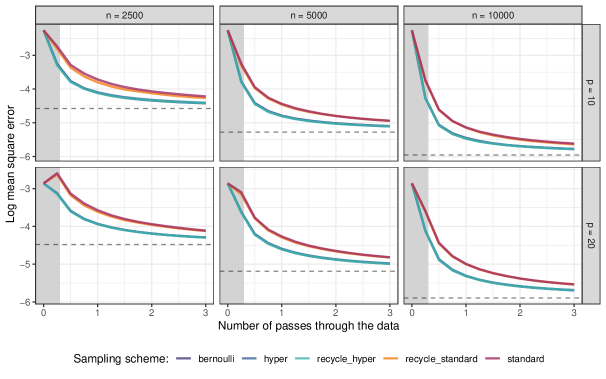
Figure 1: Ising model. Log mean square error trajectories along the optimization, grouped by $n$ and $p$. Solid lines refer to $\bar{\bm{\theta}}_{\mathcal{P}}$ under different sampling schemes. Dashed lines denote the performance of the numerical approximation of $\hat{\bm{\theta}}$. Grey areas highlight the burn-in.

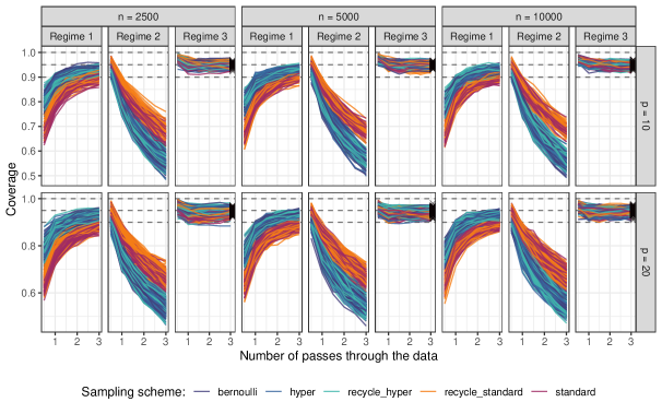
Figure 2: Ising model. Empirical coverage of confidence intervals for $\bar{\bm{\theta}}_{\mathcal{P}}$ constructed according to Theorem 1. Results are grouped by $n$ and $p$. Dashed lines highlight the nominal coverage level $95\%$. Solid lines refer to scalar elements of $\bar{\bm{\theta}}_{\mathcal{P}}$ under different sampling schemes. Dark crosses refer to scalar elements of the numerical approximation of $\hat{\bm{\theta}}$ (placed after the third pass for visualization purposes).

In this regard, Figure 2 shows that, by appropriately accounting for both sources of variability when the algorithm is stopped, it is possible to draw inference about ${\bm{\theta}}^{*}$ using $\bar{\bm{\theta}}_{\mathcal{P}}$, whatever the choice of $\mathcal{P}$. It presents the empirical coverage levels obtained by constructing confidence intervals following the covariance matrices outlined in Theorem 1 under the three asymptotic regimes. As predicted by the theory, one should use Regime 1 when $T_{n}=\omega(n)$, and Regime 2 in the opposite scenario, $T_{n}=o(n)$. However, in practice, Regime 3 is the recommendable choice because it directly compounds both the uncertainty of the optimization and the data sampling variability. As a reference, under Regime 3, Figure 2 reports the empirical coverage levels obtained by constructing confidence intervals for the numerical optimizer estimating the asymptotic covariance matrix in (6).

For space reasons, computational times are reported in Appendix C. Briefly, taking advantage of a recycling window of iterations is highly beneficial implementation-wise, especially with diverging $n$. In particular, it allows recycle_hyper to be computationally competitive with standard and recycle_standard while being systematically more efficient in statistical terms, whatever the choice of $T_{n}$ (and of $\eta_{0}$, as remarked in the additional experiments reported in the Appendix).

4.2 Experiments for Example 2

While the previous example clearly shows the statistical convenience of relying on $\mathcal{P}_{2}$ or $\mathcal{P}_{3}$ rather than $\mathcal{P}_{1}$, the experiments in this second example illustrate how these differences vary based on the model considered. That is, since the discrepancy in the asymptotic covariance of the considered estimators depends on the matrices $\bm{H}$ and $\bm{J}$, such a gap can be more or less evident according to the model analysed. Compared to the previous example, this difference is much more apparent in the gamma frailty model, as illustrated below.

Figure 3: Gamma frailty model. Log mean square error trajectories grouped by $n$ and $p$. Solid lines refer to $\bar{\bm{\theta}}_{\mathcal{P}}$ under different sampling schemes. Dashed lines denote the performance of the numerical approximation of $\hat{\bm{\theta}}$. Grey areas highlight the burn-in.

Similarly to the previous experiments, we assess the performances of Algorithm 1 for $n\in\{2500,5000,10000\}$ and $p\in\{20,30\}$. Note that, from $p=20$ to $p=30$, the dimension of the parameter space goes from $d=22$ to $d=32$ while the computational burden per iteration more than doubles since $K$ increases from $K=190$ to $K=435$. Given the large number of likelihood contributions considered compared to the Ising model, we only assess the performances of recycle_standard and recycle_hyper, and not their exact versions. In particular, $\mathcal{P}_{3}$ is the sampling scheme suffering the most from the hefty $K$. Accordingly, we increase the recycling window length to $l=500$ for both estimators to have competitive computational times. For completeness, Appendix C provides further experiments showing how different values of $l$ lead to comparable estimates for recycle_hyper while having massive impacts on computational times.

We set the true parameters as $\xi=0.25$ and $\rho=0.5$, while $\lambda_{j}$ equals $0.25$ if $j$ is even and $-0.25$ if odd. As in the previous experiments, optimization always starts from the null vector and all the performance criteria are evaluated for different running lengths of the algorithm. Results are reported setting $\eta_{0}=2$, whereas additional experiments for different values of $\eta_{0}$ are available in Appendix C. Similarly to previous experiments, the value of $\eta_{0}$ shown is the stepsize minimising the mean square error performance at $T_{n}=3n$ of recycle_standard in the most challenging setting, i.e. $n=2500,p=30$.

Figure 3 shows the trajectories along the optimization of the log mean square error for the proposed estimators. Similarly to the Ising model, the MSE differences are due to the different asymptotic variabilities implied by $\mathcal{P}_{1}$ and $\mathcal{P}_{3}$, but in this case they are more pronounced. The estimates based on $\mathcal{P}_{3}$ exhibit a sharp drop at the beginning of the optimization and reach the performance of the numerical estimator almost always after one pass through the data. For the estimates based on $\mathcal{P}_{1}$, the convergence is much slower and does not match the numerical approximation even after the maximum length tested of three passes. What happens is that the optimization noise of $\mathcal{P}_{3}$ drops almost immediately to negligible levels, leading the variance of $\bar{\bm{\theta}}_{\mathcal{P}_{3}}$ to closely overlap with the one from numerical estimation. The noise generated by $\mathcal{P}_{1}$, instead, persists much longer, and this translates into higher variances for the stochastic estimates throughout the optimization and, consequently, higher MSE.

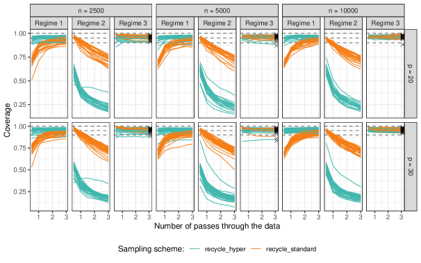
Figure 4: Gamma frailty model. Empirical coverage of confidence intervals for $\bar{\bm{\theta}}_{\mathcal{P}}$ constructed under Theorem 1. Results are grouped by $n$ and $p$. Dashed lines highlight the nominal coverage level $95\%$. Solid lines refer to scalar elements of $\bar{\bm{\theta}}_{\mathcal{P}}$ under different sampling schemes. Dark crosses refer to scalar elements of the numerical approximation of $\hat{\bm{\theta}}$ (placed after the third pass for visualization purposes).

As in previous experiments, Figure 4 shows the empirical coverage performance of $95\%$ confidence intervals constructed using the asymptotic matrices outlined in Theorem 1. Differently from what happens with the Ising model, given the low optimization noise generated by $\mathcal{P}_{3}$ in this gamma frailty example, inference for estimates based on such a sampling scheme can also run reliably in Regime 1. At the same time, it is never possible under Regime 2. However, again, Regime 3 shows up as the most reliable choice for $\bar{\bm{\theta}}_{\mathcal{P}}$ in practice, whatever the sampling scheme chosen.

As in the previous case, details about the computation times are left to Appendix C. Briefly note that recycle_standard is faster than recycle_hyper when both are stopped at the same $T_{n}$. However, the simulations show that even after $T_{n}=n$, recycle_hyper is already closer to the numerical estimates than recycle_standard at $T_{n}=3n$. Thus, it represents a more efficient alternative to recycle_standard both computationally and statistically. In addition to this, the low variability of the recycle_hyper also allows for larger stepsizes than what shown here, which permits stopping the optimization even earlier than $T_{n}=n$. See Appendix C for further experiments.

5 A Network Analysis of Mental Health Data

To illustrate the convenience of the proposed methodology, we consider an application of the Ising model to the mental health data from the Epidemiologic Survey on Alcohol and Related Conditions (NESARC) - Wave 1. The NESARC is a nationally representative survey of the United States adult population, which gathered data on alcohol behavior and mental health disorders from April 2001 to June 2002 (Grant et al., 2003).

Our modelling approach refers to the typical point of view of network psychometrics (see e.g. Epskamp et al., 2018; Borsboom, 2022; Zhang & Chen, 2023). That is, we consider symptoms as nodes of an unknown graph, while direct symptom-to-symptom interactions are encoded as edges and need to be estimated from the data. We select $p=32$ items related to antisocial disorders, high mood, low mood, panic and personality disorders, and social and other specific forms of phobia. Therefore, the dimension of the parameter space is $d=528$. The items have been selected among the ones with the lowest missing response rates, avoiding screening items and related ones, and the remaining observations with missing values were discarded from the analysis, leaving the dataset with a total of $31,826$ respondents. See Appendix D for the description of the 32 items considered. We hold out $10\%$ of the available observations as a validation set to monitor the out-of-sample behavior of the negative composite log-likelihood during the iterations. The training partition retains answers on $n=28,643$ observations.

The model is estimated using the hypergeometric sampling of Definition 3. Given the large sample size, we set the recycling window at $l=1,000$ and burn-in period $B=0.25n$. The stepsize scheduling is defined by $c=.501$ and $\eta_{0}$ chosen by keeping on halving an initial proposal until the holdout negative composite log-likelihood performance ceases improving when evaluated at $T_{n}=n$. The selected value is $\eta_{0}=5$. After every $0.25n$ iterations, the algorithm performs a new evaluation of the holdout negative log-likelihood. When the improvement falls under $0.1\%$, the algorithm stops. In our case, it stops at $T_{n}=1.75n$. The full estimation procedure, including the initial stepsize selection, took almost $15$ seconds when run on a single core of a personal laptop. As a benchmark, on the same hardware, the numerical estimator took more than half an hour to converge, providing similar results.

At the end of the stochastic estimation, the asymptotic standard errors are computed by estimating the covariance matrix of $\bar{\bm{\theta}}_{\mathcal{P}_{3}}$ under Regime 3 of Theorem 1 using the usual sample estimators of $\bm{H}$ and $\bm{J}$. To investigate the structure of the estimated graphical model, all the $d$ parameters are tested against the null hypothesis of being zero. The resulting p-values are then adjusted via the Holm correction (Holm, 1979) in order to control for the family-wise error rate across the $d$ hypothesis at level $0.01$. The procedure identifies $17.1\%$ of the possible edges as statistically significant, as visualized in Figure 5.

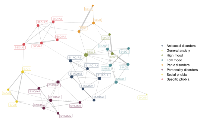
Figure 5: Graphical structure of mental health disorders. Node colors refer to specific survey areas. Solid and dashed lines stand for positive and negative estimated edges. Edge width is proportional to the absolute estimated coefficient.

The identified graphical structure highlights how symptoms related to the same disorder tend to cluster together with dense positive connections. Instead, relationships among different disorders are less strict, with some of them being slightly negative. Furthermore, the sparsity induced by the non-significance of a large number of edges allows for providing conditional independence statements among symptom areas. For example, panic disorders are conditionally independent of the rest of the graph, given the specific phobias and mood disorders areas. The same can be said for the social phobia area, which is independent of mood disorders, for example, when conditioned on personality disorders and other specific types of phobias. Similar reasoning can be used in investigating symptoms belonging to the same area. For example, item S6Q2 concerns the experience of feeling erroneously in danger after a panic attack. This symptom is isolated from the others when the remaining two items related to panic attacks, S6Q1 and S643, are taken into account. In particular, such items refer to experiencing panic episodes for no real reason and misinterpreting nerves as a heart attack. Finally, it can also happen that single items separate two specific portions of the graph. That is the case of the node S4CQ1, which concerns having experienced two or more years of depression and separates from the rest of the symptoms item S9Q1B, which is related to experiencing six months or longer of nervousness about everyday problems.

6 Discussion

When the optimization noise is non-negligible, it is crucial to properly quantify the uncertainty around stochastic approximations if the goal is to run valid frequentist inference about true parameters. We show how the asymptotic variance of such estimators compounds two sources of uncertainty: the sampling variability of the data and the noise injected in the procedure by the SGs. We focus on optimizing composite likelihoods and suggest constructing the SGs using a hypergeometric sampling of sub-likelihood contributions because of its statistical and computational efficiencies. The resulting estimator is a flexible inferential tool that can be highly beneficial from a practical perspective, given the widespread use of composite likelihood modelling strategies in applied statistics. Various extensions of the proposed method are possible by expanding the scope of the parameter update in Algorithm 1. A first straightforward broadening relates to quasi-Newton alternatives of standard stochastic gradient descent (Byrd et al., 2011). Such extensions can be quite effective in practice because of adapting the stepsize to the different scales of each parameter, which typically improves the convergence of the estimator. Some non-exhaustive examples of quasi-Newton stochastic updates can be found in Bordes et al. (2009) and Byrd et al. (2016). A second forthright extension enriches the update step to account for proximal operators, allowing the incorporation of non-differentiable terms in the estimation, like projections and lasso penalties, as investigated in Atchadé et al. (2017) and Zhang & Chen (2022).

Nevertheless, it is worth noting that our current proposal still has some limits, especially related to inference with increasing dimensions of the parameter space. From a computational point of view, it leaves the issue of computing $\bm{H}^{-1}$ and $\bm{J}$ untouched. However, an accurate estimate of both $\bm{H}^{-1}$ and $\bm{J}$ is needed to construct reliable confidence intervals. Estimating such quantities can be highly involved computationally with large numbers of parameters, particularly because of the matrix inversion needed. Furthermore, this work focuses on settings where traditional frequentist estimation is theoretically adequate but computationally inconvenient, i.e. moderate parameter spaces but still much larger sample sizes. Further work is needed to extend the current theoretical framework to settings where a regularization term is needed to identify the parameters of interest. Carrying out inference in such settings is not straightforward because of the bias introduced by the regularization. In this regard, we are exploring possible solutions based on the recent advances in debiasing techniques for lasso-based estimators, which are quickly gaining traction both in offline settings (Janková & van de Geer, 2018) and with streaming data (Luo et al., 2021; Han et al., 2021). Addressing such theoretical barriers can thus unlock composite likelihood inference on higher dimensions than the ones considered in this paper.

Appendix A Regularity conditions for composite likelihood asymptotics

The following assumptions are standard regularity conditions typically assumed to be verified when dealing with misspecified models and, in our case composite likelihoods (see Varin & Vidoni 2005, White 1982). While not specifically related to the algorithm proposed in this paper, we report them here since we assume the composite likelihood estimator to behave regularly.

Assumption 5.

The parameter space ${\bm{\theta}}$ is a compact subset of $\mathbb{R}^{d}$ and $c\ell({\bm{\theta}};y)\neq c\ell({\bm{\theta}}^{\prime};\bm{y})$ for ${\bm{\theta}}^{\prime}\neq{\bm{\theta}}$ with ${\bm{\theta}},{\bm{\theta}}^{\prime}\in{\bm{\theta}}$ , for every $\bm{y}\in\mathcal{Y}$. The true parameter value ${\bm{\theta}}^{*}$ is an interior point of ${\bm{\theta}}$ and verifies $E_{\bm{Y}}\left\{u(\bm{\theta}^{*};\bm{Y})\right\}=0$.

Assumption 6.

Each log sub-likelihood $\ell_{k}({\bm{\theta}};\bm{y})$ is twice differentiable and continuous in ${\bm{\theta}}$, for every $\bm{y}\in\mathcal{Y}$. Furthermore, $\lvert\ell_{k}({\bm{\theta}};\bm{y})\rvert$, $\lVert\nabla\ell_{k}({\bm{\theta}};\bm{y})\rVert$ and $\lVert\nabla^{2}\ell_{k}({\bm{\theta}};\bm{y})\rVert$ to be dominated by functions of $\bm{y}$ integrable with respect to $g(\bm{Y})$ for all ${\bm{\theta}}\in{\bm{\theta}}$. Furthermore the matrices $\bm{H}=E_{\bm{Y}}\left\{-\nabla u(\bm{\theta}^{*};\bm{Y})\right\}$ and $\bm{J}=\text{Var}_{\bm{Y}}\left\{u({\bm{\theta}}^{*};\bm{Y})\right\}$ exist and are positive definite.

Note also that by the smoothness condition required in Assumption 6, we can exchange differentiation and integral operator such that, with $c\ell(\bm{\theta})=n^{-1}E_{\bm{Y}}\{-c\ell_{n}(\bm{\theta})\}$, it holds $\nabla c\ell(\bm{\theta})=n^{-1}E_{\bm{Y}}\{-\nabla c\ell_{n}(\bm{\theta})\}$ and $\nabla^{2}c\ell(\bm{\theta})=n^{-1}E_{\bm{Y}}\{-\nabla^{2}c\ell_{n}(\bm{\theta}))\}$.

Appendix B Technical proofs

B.1 Proof of Proposition 1

In the following, we prove Proposition 1 by verifying all the conditions needed by the convergence part of Theorem 2 in Polyak & Juditsky (1992). While we closely replicate their proof strategy, we still need to adjust for the fact we want to directly approximate ${\bm{\theta}}^{*}$ rather than ${\hat{\bm{\theta}}}$. Consider the decomposition $n^{-1}{\bm{S}_{t}}=\nabla c\ell(\bm{\theta})+{\bm{\xi}_{n,t}}({\bm{\theta}},{\bm{W}_{t}})$. Additionally, we can write ${\bm{\xi}_{n,t}}({\bm{\theta}},{\bm{W}_{t}})={\bm{\xi}_{n,t}}({\bm{\theta}}^{*},{\bm{W}_{t}})-{\bm{\zeta}_{t}}({\bm{\theta}}_{t-1};{\bm{W}_{t}})$. For conciseness, in the following, we use the notation ${\bm{\xi}_{t}}={\bm{\xi}_{n,t}}({\bm{\theta}}_{t-1},{\bm{W}_{t}})$ , ${\bm{\xi}_{t}}^{*}={\bm{\xi}_{n,t}}({\bm{\theta}}^{*},{\bm{W}_{t}})$ and ${\bm{\zeta}_{t}}={\bm{\zeta}_{t}}({\bm{\theta}}_{t-1},{\bm{W}_{t}})$.

The following Lemmata 1 and 2 guarantee Assumptions 3.1 and 3.2 in Polyak & Juditsky 1992 to be verified.

Lemma 1.

Under Assumptions 2, 3, 5, 6, there exist a function $G({\bm{\theta}}):{\bm{\theta}}\rightarrow\mathbb{R}$ such that for some $C^{(1)}>0$, $C^{(2)}>0$, $C^{(3)}>0$, $C^{(4)}>0$ and all ${\bm{\theta}},{\bm{\theta}}^{\prime}\in\Theta$, it holds that

$$G({\bm{\theta}})\geq C^{(1)}\lVert{\bm{\theta}}\rVert^{2};$$ (9)

$$\lVert\nabla G({\bm{\theta}})-\nabla G({\bm{\theta}}^{\prime})\rVert\leq C^{(2)}\lVert{\bm{\theta}}-{\bm{\theta}}^{\prime}\rVert;$$ (10)

$$\nabla G({\bm{\theta}}-{\bm{\theta}}^{*})^{\top}\nabla c\ell(\bm{\theta})>0\;\text{for all ${\bm{\theta}}\neq{\bm{\theta}}^{*}$}$$ (11)

$$\nabla G({\bm{\theta}}-{\bm{\theta}}^{*})^{\top}\nabla c\ell(\bm{\theta})\geq C^{(3)}G({\bm{\theta}}-{\bm{\theta}}^{*})\text{ for all $\|{\bm{\theta}}-{\bm{\theta}}^{*}\rVert\leq C^{(4)}$}.$$ (12)

Proof.

Consider ${\bm{\theta}}^{*}$ satisfying Assumption 5. Furthermore, let 6 hold such that we can define $c\ell(\bm{\theta})$ and $\nabla c\ell(\bm{\theta})$ as in Appendix A. By Assumption 3, $c\ell(\bm{\theta})$ is strictly convex since

$$c\ell({\bm{\theta}}^{\prime})-c\ell(\bm{\theta})=E\left[\sum_{k=1}^{K}\{\ell_{k}({\bm{\theta}}^{\prime};\bm{Y})-\ell_{k}({\bm{\theta}};\bm{Y})\}\right]\geq\nabla c\ell({\bm{\theta}}^{\prime})^{\top}({\bm{\theta}}^{\prime}-{\bm{\theta}})+\frac{\mu}{2}\lVert{\bm{\theta}}^{\prime}-{\bm{\theta}}\rVert^{2}$$

with ${\bm{\theta}},{\bm{\theta}}^{\prime}\in{\bm{\theta}}$, $\mu=\sum_{k}\mu_{k}>0$. Then, by defining $G({\bm{\theta}})=c\ell({\bm{\theta}}+{\bm{\theta}}^{*})-c\ell({\bm{\theta}}^{*})$, we get $G({\bm{\theta}})\geq\nabla c\ell({\bm{\theta}}^{*})^{\top}{\bm{\theta}}+\frac{\mu}{2}\lVert{\bm{\theta}}\rVert^{2}=C^{(1)}\lVert{\bm{\theta}}\rVert^{2}$, with $C^{(1)}=\sum_{k}\mu_{k}/2$. Furthermore, note that $\lVert\nabla G({\bm{\theta}})-\nabla G({\bm{\theta}}^{\prime})\rVert=\lVert\nabla c\ell(\bm{\theta})-\nabla c\ell({\bm{\theta}}^{\prime})\rVert$. Since $\lVert.\rVert$ is convex, by Assumption 2, we can write

$$\lVert\nabla c\ell(\bm{\theta})-\nabla c\ell({\bm{\theta}}^{\prime})\rVert\leq E\lVert\nabla c\ell({\bm{\theta}};\bm{Y})-\nabla c\ell({\bm{\theta}}^{\prime};\bm{Y})\rVert\leq\sum_{k}L_{1,k}\lVert{\bm{\theta}}-{\bm{\theta}}^{\prime}\rVert=C^{(2)}\lVert{\bm{\theta}}-{\bm{\theta}}^{\prime}\rVert$$

with $C^{(2)}=K\max_{k}\{L_{1,k}\}$. Finally, by Polyak-Lojasiewicz inequality it holds that

$$\nabla G({\bm{\theta}}-{\bm{\theta}}^{*})^{\top}\nabla c\ell(\bm{\theta})=\lVert\nabla c\ell(\bm{\theta})\rVert^{2}\geq 2\mu\left(c\ell(\bm{\theta})-c\ell({\bm{\theta}}^{*})\right)=C^{(3)}G({\bm{\theta}}-{\bm{\theta}}^{*})>0,$$

with $C^{(3)}=2\mu$ which completes the proof. ∎

Lemma 2.

Under Assumptions 5 and 6, there exists a positive definite matrix $\bm{M}\in\mathbb{R}^{d}\times\mathbb{R}^{d}$ and some constants $C^{(5)}<\infty$, $C^{(6)}>0$, $0<C^{(7)}\leq 1$, such that $\lVert\nabla c\ell(\bm{\theta})-\bm{M}({\bm{\theta}}-{\bm{\theta}}^{*})\rVert\leq C^{(5)}\lVert{\bm{\theta}}-{\bm{\theta}}^{*}\rVert^{1+C^{(7)}}$ for all $\lVert{\bm{\theta}}-{\bm{\theta}}^{*}\rVert\leq C^{(6)}>0$.

Proof.

Let $\{{\bm{\theta}}_{t}\}_{\infty}$ be an arbitrary infinite sequence of points in ${\bm{\theta}}$ increasingly close to ${\bm{\theta}}^{*}$, such that for each $C^{(6)}>0$ there exists a $t_{0}$ such that $\lVert{\bm{\theta}}_{t}-{\bm{\theta}}^{*}\rVert\leq C^{(6)}$ for all $t>t_{0}$. Then, the standard regularity conditions in Assumptions 5, 6 allow us to take the first-order Taylor’s expansion of the gradient of the composite log-likelihood around ${\bm{\theta}}^{*}$, such that

$$\nabla c\ell_{n}({\bm{\theta}}_{t})=\nabla c\ell_{n}({\bm{\theta}}^{*})+\nabla^{2}c\ell_{n}({\bm{\theta}}^{*})({\bm{\theta}}_{t}-{\bm{\theta}}^{*})+r_{1}$$ (13)

where the remainder term $\lVert r_{1}\rVert$ is an $O(n)$ times an $O(\lVert{\bm{\theta}}_{t}-{\bm{\theta}}^{*}\rVert^{2})$ by definition. By taking the expected value of the negative of both sides and dividing by $n$, we get $\lVert\nabla c\ell({\bm{\theta}}_{t})-\nabla^{2}c\ell({\bm{\theta}}^{*})({\bm{\theta}}_{t}-{\bm{\theta}}^{*})\rVert=O(\lVert{\bm{\theta}}_{t}-{\bm{\theta}}^{*}\rVert^{2})$, then, by construction, it holds that

$$\lVert\nabla c\ell({\bm{\theta}}_{t})-\nabla^{2}c\ell({\bm{\theta}}^{*})({\bm{\theta}}_{t}-{\bm{\theta}}^{*})\rVert\leq C^{(5)}\lVert{\bm{\theta}}_{t}-{\bm{\theta}}^{*}\rVert^{2}$$ (14)

for some $C^{(5)}$ large enough, $\lVert{\bm{\theta}}_{t}-{\bm{\theta}}^{*}\rVert\leq C^{(6)}$ and $t>t_{0}$. Therefore, the lemma is proven with $C^{(5)}$, $\bm{M}=\nabla^{2}c\ell({\bm{\theta}}^{*})=\bm{H}$ and $C^{(7)}=1$. ∎

Lemma 3 guarantees that Assumption 3.3 in Polyak & Juditsky (1992) is satisfied, apart from its Lindeberg condition. While the remaining results are needed to prove the convergence of the algorithm, the Lindeberg condition is needed to call the central limit theorem for martingales. However, as will be clear in B, our special setting requires relying on the central limit theorem for exchangeable random variables in Blum et al. (1958).

Lemma 3.

Under Assumptions 1-6, the sequence $\left\{{\bm{\xi}_{n,t}}\right\}_{T_{n}}$ is a martingale difference sequence, given the filtration $\mathscr{F}_{n,t-1}$, i.e.
$E\left\{{\bm{\xi}_{n,t}}|\mathscr{F}_{n,t-1}\right\}=0$ a.s., $E\left\{\lVert{\bm{\xi}_{n,t}}\rVert|\mathscr{F}_{n,t-1}\right\}<\infty$ and it holds that
$E\left\{\lVert{\bm{\xi}_{n,t}}\rVert^{2}|\mathscr{F}_{n,t-1}\right\}+\lVert\nabla c\ell({\bm{\theta}}_{t-1})\rVert^{2}\leq C^{(8)}(1+\lVert{\bm{\theta}}_{t-1}\rVert^{2})\;a.s.$ for some $C^{(8)}>0$.

Proof.

Let Assumptions 5 and 6 hold such that we can use ${\bm{\theta}}^{*}$, $c\ell(\bm{\theta})$ and $\nabla c\ell(\bm{\theta})$ as defined in Appendix A. The null expected value of the sequence follows automatically since, at each iteration $t$, for all ${\bm{\theta}}\in\Theta$, we have

$$E\left\{{\bm{\xi}_{n,t}}|\mathscr{F}_{n,t-1}\right\}=n^{-1}E\left\{{\bm{S}_{t}}|\mathscr{F}_{n,t-1}\right\}-\nabla c\ell({\bm{\theta}}_{t-1})=0.$$

Now, let us focus on the expected norm of the values in the sequence. First, recall that, with Assumption 2 holding, $\lVert\nabla c\ell({\bm{\theta}}_{t-1})\rVert\leq C^{(2)}\lVert{\bm{\theta}}_{t-1}-{\bm{\theta}}^{*}\rVert$, as shown in the proof of Lemma 1. Furthermore, since by Assumption 1 it holds $\lvert W_{i,k,t}\rvert^{2}=\lvert W_{i,k,t}\rvert=W_{i,k,t}$, we can bound the expected norm of the stochastic gradient with $E\left\{\lVert{\bm{S}_{t}}\rVert|\mathscr{F}_{n,t-1}\right\}$ using Assumption 2, namely

$$E\left\{\lVert n^{-1}{\bm{S}_{t}}\rVert|\mathscr{F}_{n,t-1}\right\}\leq n^{-1}\gamma_{1}^{-1}\sum_{i}\sum_{k}E\left\{W_{i,k,t}\right\}E\left\{\lVert\nabla\ell_{k}({\bm{\theta}}_{t-1};Y_{i})\rVert|\mathscr{F}_{n,t-1}\right\}$$

$$\leq Kn^{-1}\gamma_{1}^{-1}\max_{k}\left\{C_{k}\right\}\left(1+\lVert{\bm{\theta}}_{t-1}\rVert\right)=C^{(9)}\left(1+\lVert{\bm{\theta}}_{t-1}\rVert\right),$$

where $C^{(9)}=Kn^{-1}\gamma_{1}^{-1}\max_{k}\left\{C_{k}\right\}>0$. Therefore, it follows $E\left\{\lVert{\bm{\xi}_{n,t}}\rVert|\mathscr{F}_{n,t-1}\right\}\leq C^{(9)}\left(1+\lVert{\bm{\theta}}_{t-1}\rVert\right)+C^{(2)}\lVert\Delta_{t-1}\rVert<\infty$, where ${\bm{\Delta}}_{t-1}={\bm{\theta}}_{t-1}-{\bm{\theta}}^{*}$. Similarly, we can bound the expected squared norms with

$$E\left\{\lVert n^{-1}{\bm{S}_{t}}\rVert^{2}|\mathscr{F}_{n,t-1}\right\}\leq 2n^{-2}\gamma_{1}^{-2}\sum_{i}\sum_{k}E\left\{W_{i,k,t}\right\}E\left\{\lVert\nabla\ell_{k}({\bm{\theta}}_{t-1};Y_{i})\rVert^{2}|\mathscr{F}_{n,t-1}\right\}$$

$$\leq 2Kn^{-2}\gamma_{1}^{-2}\max_{k}\left\{C_{k}\right\}\left(1+\lVert{\bm{\theta}}_{t-1}\rVert^{2}\right)=C^{(10)}\left(1+\lVert{\bm{\theta}}_{t-1}\rVert^{2}\right),$$

where $C^{(10)}=2Kn^{-2}\gamma_{1}^{-2}\max_{k}\left\{C_{k}\right\}>0$, and

$$\lVert\nabla c\ell({\bm{\theta}}_{t-1})\rVert^{2} \leq 2\sum_{k}L_{1,k}^{2}\lVert{\bm{\Delta}}_{t-1}\rVert^{2}\leq C^{(11)}\lVert{\bm{\Delta}}_{t-1}\rVert^{2}$$

with $C^{(11)}=2K\max_{k}\{L_{1,k}^{2}\}>0$. Therefore,

$$E\left\{\lVert{\bm{\xi}_{n,t}}\rVert^{2}|\mathscr{F}_{n,t-1}\right\}+\lVert\nabla c\ell({\bm{\theta}}_{t-1})\rVert^{2}\leq 2E\left\{\lVert n^{-1}{\bm{S}_{t}}\rVert^{2}|\mathscr{F}_{n,t-1}\right\}+3\lVert\nabla c\ell({\bm{\theta}}_{t-1})\rVert^{2}$$

$$\leq 2C^{(10)}\left(1+\lVert{\bm{\theta}}_{t-1}\rVert^{2}\right)+3C^{(11)}\lVert{\bm{\theta}}_{t-1}\rVert^{2}+3C^{(11)}\lVert{\bm{\theta}}^{*}\rVert^{2}\leq C^{(8)}\left(1+\lVert{\bm{\theta}}_{t-1}\rVert^{2}\right)$$

with $C^{(8)}=\max\{2C^{(10)}+3C^{(11)},3C^{(11)}\lVert{\bm{\theta}}^{*}\rVert^{2}\}>0$.

With Lemmata 1-3 and Assumption 4 holding, all the conditions needed for Parts 1 and 2 of the proof of Theorem 2 in Polyak & Juditsky (1992), which guarantee the almost sure convergence of $\bar{\bm{\theta}}_{T_{n}}$ to ${\bm{\theta}}^{*}$ are satisfied. In addition, we further report two useful results stated in Parts 1 and 2 as references for the proof of Theorem 1 in Appendix B. For all $\epsilon>0$ and some $C,C^{*}>0$ it holds that

$$P(\sup_{t}\lVert{\bm{\Delta}}_{t}\rVert\leq C)=1-\epsilon;$$ (15)

$$E\lVert{\bm{\Delta}}_{t}\rVert^{2}\mathbb{I}(\tau_{C}>t)\leq C^{*}\eta_{t};$$ (16)

with $\tau_{C}=\inf\{t\geq 1\;\text{such that}\;\lVert{\bm{\Delta}}_{t}\rVert>C\}$. ∎

B.2 Proof of Theorem 1

Lemma 4.

Under Assumptions 1 and 2, it holds that $E\lVert{\bm{\zeta}_{n,t}}\rVert\leq CE\lVert{\bm{\Delta}}_{t}\rVert$ and $E\{\lVert{\bm{\zeta}_{n,t}}\rVert^{2}\}\leq CE\{\lVert{\bm{\Delta}}_{t}\rVert^{2}\}$ for some $0<C<\infty.$

Proof.

From Assumption 2, we can bound the norm of ${\bm{\zeta}_{n,t}}$ with

$$\lVert{\bm{\zeta}_{n,t}}\rVert\leq\gamma_{1}^{-1}\sum_{i}\sum_{k}\lvert W_{i,k,t}\rvert\lVert\nabla\ell_{k}({\bm{\theta}}_{t-1})-\nabla\ell_{k}({\bm{\theta}}^{*})\rVert\leq\gamma_{1}^{-1}\sum_{i}\sum_{k}\lvert W_{i,k,t}\rvert L_{1,k}\lVert{\bm{\Delta}}_{t-1}\rVert$$

Since, by Assumption 1, it holds $\lvert W_{i,k,t}\rvert^{2}=\lvert W_{i,k,t}\rvert=W_{i,k,t}$, it follows that the expected norm and norm squared can be bounded via

$$E\lVert{\bm{\zeta}_{n,t}}\rVert \leq\gamma_{1}^{-1}L_{1}E\lVert{\bm{\Delta}}_{t-1}\rVert$$

$$E\{\lVert{\bm{\zeta}_{n,t}}\rVert^{2}\} \leq 2\gamma_{1}^{-2}L_{1}^{2}E\{\lVert{\bm{\Delta}}_{t-1}\rVert^{2}\}$$

where the proof is completed with $C=\max\{\gamma_{1}^{-1}L_{1},2\gamma_{1}^{2}L_{1}^{2}\}$. ∎

Lemma 5.

Let Assumptions 1 and 4 being verified and Proposition 1 hold, then $\lim_{T_{n}}\sum_{t}^{T_{n}}E\{\lVert{\bm{\Delta}}_{t-1}\rVert^{2}\}/\sqrt{t}<\infty$.

Proof.

The following is an adaptation of Part 4 of the proof of Theorem 2 in Polyak & Juditsky (1992). By (16) we get

$$\lim_{T_{n}}\sum_{t=1}^{T_{n}}\frac{E\{\lVert{\bm{\Delta}}_{t}\rVert^{2}\}\mathbb{I}(\tau_{C}>T_{n})}{\sqrt{t}}\leq\lim_{T_{n}}\sum_{t=1}^{T_{n}}\frac{C^{*}\eta_{t}}{\sqrt{t}}<\infty,$$

since $\sum_{t}^{\infty}{\eta_{t}}/\sqrt{t}<\infty$ by Assumption 4. Note that, from (15) follows that $E\{\lVert{\bm{\Delta}}_{t}\rVert^{2}\}\leq C^{2}$. Therefore we can replace $E\{\lVert{\bm{\Delta}}_{t}\rVert^{2}\}\mathbb{I}(\tau_{C}>T_{n})$ with $E\{\lVert{\bm{\Delta}}_{t}\rVert^{2}\}$, since for all $t<T_{n}$ we get the upper bound $C^{2}$ in both cases. Then, it finally holds

$$\lim_{T_{n}}\sum_{t=1}^{T_{n}}\frac{E\{\lVert{\bm{\Delta}}_{t}\rVert^{2}\}}{\sqrt{t}}<\infty,$$

which completes the proof. ∎

Proposition 2.

Let Assumptions 1-6 be satisfied. Then, by defining the average error of the algorithm as $\bar{\bm{\Delta}}_{t}=t^{-1}\sum_{j=1}^{t}{\bm{\Delta}}_{j}$ with ${\bm{\Delta}}_{t}={\bm{\theta}}_{t}-{\bm{\theta}}^{*}$, it holds that

• Regime 1: If $\alpha=0$, then

  $$\sqrt{n}\bar{\bm{\Delta}}_{T_{n}}=\frac{\sqrt{n}}{T_{n}}\sum_{t=1}^{T_{n}-1}{\bm{H}}^{-1}{\bm{\xi}_{n,t}}({\bm{\theta}}^{*},{\bm{W}_{t}})+o_{p}(1),$$

• Regime 2: If $\alpha=1$, then

  $$\sqrt{T_{n}}\bar{\bm{\Delta}}_{T_{n}}=\frac{\sqrt{T_{n}}}{T_{n}}\sum_{t=1}^{T_{n}-1}{\bm{H}}^{-1}{\bm{\xi}_{n,t}}({\bm{\theta}}^{*},{\bm{W}_{t}})+o_{p}(1),$$

• Regime 3: If $0<\alpha<1$, then

  $$\sqrt{T_{n}+n}\bar{\bm{\Delta}}_{T_{n}}=\frac{\sqrt{T_{n}+n}}{T_{n}}\sum_{t=1}^{T_{n}-1}{\bm{H}}^{-1}{\bm{\xi}_{n,t}}({\bm{\theta}}^{*},{\bm{W}_{t}})+o_{p}(1),$$

where $T_{n}\rightarrow\infty$ as $n\rightarrow\infty$.

Proof.

Consider the iterated decomposition $n^{-1}{\bm{S}_{t}}=\nabla c\ell({\bm{\theta}}_{t-1})+{\bm{\xi}_{n,t}}$, $\nabla c\ell({\bm{\theta}}_{t-1})=H{\bm{\Delta}}_{t}+\bm{r}_{t}$ and ${\bm{\xi}_{n,t}}={\bm{\xi}_{n,t}^{*}}+{\bm{\zeta}_{t}}$ such that $n^{-1}{\bm{S}_{t}}=\bm{H}{\bm{\Delta}}_{t}+{\bm{r}_{t}}+{\bm{\xi}_{n,t}^{*}}+{\bm{\zeta}_{n,t}}$. The algorithm update can be then rewritten as

$${\bm{\Delta}}_{t}={\bm{\Delta}}_{t-1}-{\eta_{t}}(\bm{H}{\bm{\Delta}}_{t-1}+{\bm{r}_{t}}+{\bm{\xi}_{n,t}^{*}}+{\bm{\zeta}_{n,t}}).$$

We proceed assuming $0<\alpha<1$. Then, the other two cases follow similarly. Note that, in such an asymptotic regime, $(T_{n}+n)/T_{n}\xrightarrow[n]{}1/(1-\alpha)$, which is a positive finite constant. Under Assumptions 4 and 6, by Lemmata 1 and 2 in Polyak & Juditsky (1992), we can write the average error of the algorithm as

$$\sqrt{T_{n}+n}\bar{\bm{\Delta}}_{T_{n}} =\frac{\sqrt{T_{n}+n}}{T_{n}\eta_{0}}\bm{\alpha}_{0}^{(T_{n})}{\bm{\Delta}}_{0}+\frac{\sqrt{T_{n}+n}}{T_{n}}\bm{H}^{-1}\sum_{t=1}^{T_{n}-1}{\bm{\xi}_{n,t}^{*}}$$ (17)

$$+\frac{\sqrt{T_{n}+n}}{T_{n}}\bm{H}^{-1}\sum_{t=1}^{T_{n}-1}{\bm{\zeta}_{t}}+\frac{\sqrt{T_{n}+n}}{T_{n}}\sum_{t=1}^{T_{n}-1}\bm{\alpha}_{t}^{(T_{n})}{\bm{r}_{t}}$$

$$+\frac{\sqrt{T_{n}+n}}{T_{n}}\sum_{t=1}^{T_{n}-1}\bm{\beta}_{t}{\bm{\xi}_{n,t}}$$

$$=\bm{I}^{(0)}+\bm{I}^{(1)}+\bm{I}^{(2)}+\bm{I}^{(3)}+\bm{I}^{(4)}$$ (18)

with $\bm{\alpha}_{j}^{(t)}=\eta_{j}\sum_{i=j}^{t-1}\prod_{k=j+1}^{i}(\bm{I}-\eta_{k}\bm{H})$, $\bm{\beta}_{t}=\bm{\alpha}_{j}^{(t)}-{\bm{H}}^{-1}$ and $\lVert\bm{\alpha}_{j}^{(t)}\rVert\leq C$, $\lVert\bm{\beta}_{t}\rVert\leq C$, $t^{-1}\sum_{j=1}^{t-1}\lVert\bm{\beta}_{t}\rVert=0$ and $\bm{I}$ the $d$-dimensionalidentity matrix. Then, it follows directly that

$$E\{\lVert\bm{I}^{(0)}\rVert^{2}\} \leq\left(\frac{T_{n}+n}{T_{n}}\right)\frac{\lVert{\bm{\Delta}}_{0}\rVert^{2}}{\eta_{0}^{2}T_{n}}\lVert\bm{\alpha}_{0}^{(T_{n})}\rVert^{2}\leq\left(\frac{T_{n}+n}{T_{n}}\right)\frac{C}{T_{n}}\xrightarrow[n]{}0,$$

with $C=\lVert{\bm{\Delta}}_{0}\rVert^{2}\lVert\bm{\alpha}_{0}^{(T_{n})}\rVert^{2}/\eta_{0}^{2}$. Concerning $\bm{I}^{(2)}$, by Lemma 4 we can write

$$E\lVert\bm{I}^{(2)}\rVert^{2} \leq\left(\frac{T_{n}+n}{T_{n}}\right)\frac{2\lVert\bm{H}^{-1}\rVert^{2}}{T_{n}}\sum_{t=1}^{T_{n}}E\lVert{\bm{\zeta}_{t}}\rVert^{2}\leq\left(\frac{T_{n}+n}{T_{n}}\right)\frac{C}{\sqrt{T_{n}}}\sum_{t=0}^{T_{n}}\frac{E\{\lVert{\bm{\Delta}}_{t}\rVert^{2}\}}{\sqrt{t}}\xrightarrow[n]{}0,$$

where the last sum is finite, letting Lemma 5 hold. Similarly, Lemma 5 also provides the bound for the norm of $\bm{I}^{(3)}$, namely

$$E\lVert\bm{I}^{(3)}\rVert \leq\sqrt{\frac{T_{n}+n}{T_{n}}}\frac{1}{\sqrt{T_{n}}}\sum_{t}\lVert\bm{\alpha}_{t}^{(T_{n})}\rVert E\lVert{\bm{r}_{t}}\rVert\leq\sqrt{\frac{T_{n}+n}{T_{n}}}\frac{C}{\sqrt{T_{n}}}\sum_{t=1}^{T_{n}}E\{\lVert{\bm{\Delta}}_{t-1}\rVert^{2}\}$$

$$\leq\sqrt{\frac{T_{n}+n}{T_{n}}}\frac{C}{\sqrt{T_{n}}}\sum_{t=1}^{T_{n}}\sqrt{T_{n}}\frac{E\{\lVert{\bm{\Delta}}_{t-1}\rVert^{2}\}}{\sqrt{t}}\xrightarrow[n]{}0,$$

where the last bound goes to $0$ by Lemma 5 and Kronecker’s lemma. Finally, by using the bounds on $\lVert\bm{\beta}_{t}\rVert$ and the limit of their average, it follows that

$$E\{\lVert\bm{I}^{(4)}\rVert^{2}\} \leq\left(\frac{T_{n}+n}{T_{n}}\right)\frac{2}{T_{n}}\sum_{t=1}^{T_{n}}\lVert\bm{\beta}_{t}\rVert^{2}E\{\lVert\bm{\xi}_{n,t}\rVert^{2}\}\leq\left(\frac{T_{n}+n}{T_{n}}\right)\frac{C^{*}}{T_{n}}\sum_{t=1}^{T_{n}}\lVert\bm{\beta}_{t}\rVert\xrightarrow[n]{}0,$$

for some $C^{*}>0$ large enough. Therefore, the asymptotic distribution of $\bar{\bm{\Delta}}_{t}$ only depends on $\bm{I}^{(1)}$, as stated. ∎

Proof of Theorem 1: Let Assumptions 1-6 be satisfied. Furthermore, let us write

$$\bar{\bm{\xi}}^{*} =\frac{1}{T_{n}}\sum_{t=1}^{T_{n}}{\bm{\xi}_{n,t}^{*}}=\frac{1}{nT_{n}}\sum_{t=1}^{T_{n}}\sum_{i=1}^{n}\bm{S}_{i,t}^{*}=\frac{1}{n}\sum_{i=1}^{n}\bm{S}_{i}^{*},$$

where $\bm{S}_{i,t}^{*}=\gamma_{1}^{-1}\sum_{k}W_{i,k,t}\nabla\ell_{k}({\bm{\theta}}^{*};Y_{i})$ represents the contribution of the $i$-th observation to the stochastic gradient, and $\bm{S}_{i}^{*}={T_{n}}^{-1}\sum_{t}^{T_{n}}S_{i,t}^{*}$ its average along the optimisation, for $i=1,\dots,n$ and $t=1,\dots,T_{n}$. Recall that, after Assumption 1, $E\{W_{i,k,t}\}=E\{W_{i,k,t}^{2}\}=\gamma_{1}$, $E\{W_{i,k,t}W_{j,k,t}\}=\gamma_{2}$ and $E\{W_{i,k,t}W_{i,h,t}\}=\gamma_{3}$. Then, the conditional variance of $\bm{S}_{i,t}^{*}$ takes the form

$$\text{Var}_{\bm{W}|\bm{Y}}(\bm{S}_{i,t}^{*}) =\gamma_{1}^{-2}(\gamma_{1}-\gamma_{3})\sum_{k=1}^{K}\left\{\nabla\ell_{k}({\bm{\theta}}^{*};\bm{Y}_{i})\right\}\left\{\nabla\ell_{k}({\bm{\theta}}^{*};\bm{Y}_{i})\right\}^{\top}+$$

$$+\left(\gamma_{1}^{-2}\gamma_{3}-1\right)\sum_{k=1}^{K}\sum_{h=1}^{K}\left\{\nabla\ell_{k}({\bm{\theta}}^{*};\bm{Y}_{i})\right\}\left\{\nabla\ell_{h}({\bm{\theta}}^{*};\bm{Y}_{i})\right\}^{\top}.$$

and its expected value is $E_{\bm{\bm{Y}}}\text{Var}_{\bm{W}|\bm{Y}}(\bm{S}_{i,t}^{*})=\gamma_{1}^{-2}(\gamma_{1}-\gamma_{3})\bm{H}+\left(\gamma_{1}^{-2}\gamma_{3}-1\right)\bm{J}$, since

$$E_{\bm{\bm{Y}}}\left\{\sum_{k=1}^{K}\left\{\nabla\ell_{k}({\bm{\theta}}^{*};\bm{Y}_{i})\right\}\left\{\nabla\ell_{k}({\bm{\theta}}^{*};\bm{Y}_{i})\right\}^{\top}\right\} =\bm{H},$$

by exploiting the second Bartlett’s identity on the single sub-likelihood components and

$$E_{\bm{\bm{Y}}}\left\{\sum_{k=1}^{K}\sum_{h=1}^{K}\left\{\nabla\ell_{k}({\bm{\theta}}^{*};\bm{Y}_{i})\right\}\left\{\nabla\ell_{h}({\bm{\theta}}^{*};\bm{Y}_{i})\right\}^{\top}\right\} =\bm{J},$$

by definition of $\bm{J}$. Then, $\text{Var}(\bm{S}_{i}^{*})={T_{n}}^{-1}E_{{\bm{Y}}}\text{Var}_{\bm{W}|\bm{Y}}(\bm{S}_{i,t}^{*})+\bm{J}$.

In order to prove Theorem 1, we need to show the asymptotic multivariate normality of the vector $\bar{\bm{\xi}^{*}}$. We take advantage of the Central Limit Theorem for exchangeable processes outlined in Blum et al. (1958) (Theorem 2, page 227) by exploiting the conditional independence of the random vectors $\bm{S}_{1}^{*},\dots,\bm{S}_{n}^{*}$ given the weighting sequence $\bm{W}_{1},\dots,\bm{W}_{T_{n}}$. For conciseness, let us focus on Regime 3; the other two are simpler and follow similarly. With such an asymptotic regime, we need to show that

$$\sqrt{T_{n}+n}\bar{\bm{\xi}^{*}}\xrightarrow[n]{d}\mathcal{N}\left(0,\bm{V}_{\mathcal{P}}/(1-\alpha)+\bm{J}/\alpha\right).$$ (19)

We proceed by using the Cramér-Wold device, such that the problem reduces to verify that every linear combination $\bm{c}^{\top}\bar{\bm{\xi}^{*}}$, with $\bm{c}\in\mathbb{R}^{d}$, converges to the univariate normal distribution

$$\sqrt{T_{n}+n}\bm{c}^{\top}\bar{\bm{\xi}^{*}}\xrightarrow[n]{d}\mathcal{N}\left(0,\bm{c}^{\top}\bm{V}_{{\mathcal{P}}}\bm{c}/(1-\alpha)+\bm{c}^{\top}\bm{J}\bm{c}/\alpha\right).$$ (20)

Otherwise stated, if we show that (20) holds, then the Cramér-Wold Theorem implies (19) to hold as well.

Let us start by writing $\bm{c}^{\top}\bar{\bm{\xi}^{*}}=n^{-1}\sum_{i}\bm{c}^{\top}\bm{S}_{i}^{*}$. In particular, note that the scalar quantities $\bm{c}^{\top}\bm{S}_{1}^{*},\dots,\bm{c}^{\top}\bm{S}_{n}^{*}$ define a sequence of exchangeable random variables since they are i.i.d. conditioned on the values of $\bm{W}_{1},\dots,\bm{W}_{T_{n}}$. In order to apply Theorem 2 in Blum et al. (1958), we need to show for $i\neq i^{\prime}$ with $i,i^{\prime}=1,\dots,n$, that

$$(i)\quad \quad E\left\{(\bm{c}^{\top}\bm{S}_{i}^{*})(\bm{c}^{\top}\bm{S}_{i^{\prime}}^{*})\right\}=o\left(\frac{1}{n}\right);$$

$$(ii)\quad \quad\lim_{n}\text{Cov}\left\{(\bm{c}^{\top}\bm{S}_{i}^{*})^{2},(\bm{c}^{\top}\bm{S}_{i^{\prime}}^{*})^{2}\right\}=0;$$

$$(iii)\quad \quad E\left\{\lvert\bm{c}^{\top}\bm{S}_{i}^{*}\rvert^{3}\right\}=o(\sqrt{n}).$$

Since the quantities $\bm{S}_{i}^{*}$ and $\bm{S}_{i^{\prime}}^{*}$ are linearly independent, condition (i) is automatically satisfied. Note, in fact, that

$$E\left\{\bm{S}_{i}^{*}\bm{S}_{i^{\prime}}^{*}\right\} =\frac{1}{T_{n}^{2}\gamma_{1}^{2}}\sum_{t}^{T_{n}}\sum_{t^{\prime}}^{T_{n}}\sum_{k}\sum_{k^{\prime}}E\left\{W_{i,k,t}W_{i^{\prime},k^{\prime},t^{\prime}}\right\}E\left\{\nabla\ell_{k}({\bm{\theta}}^{*};\bm{Y}_{i})\nabla\ell_{k^{\prime}}({\bm{\theta}}^{*};\bm{Y}_{i^{\prime}})^{\top}\right\}=0,$$

given that $E\left\{\nabla\ell_{k}({\bm{\theta}}^{*};\bm{Y}_{i})\nabla\ell_{k^{\prime}}({\bm{\theta}}^{*};\bm{Y}_{i^{\prime}})^{\top}\right\}$ is always null as long as $\bm{Y}_{i}$ and $\bm{Y}_{i^{\prime}}$ are independent. It follows that $E\left\{(\bm{c}^{\top}\bm{S}_{i}^{*})(c^{\top}\bm{S}_{i^{\prime}}^{*})\right\}=\bm{c}^{\top}E\left\{\bm{S}_{i}^{*}\bm{S}_{i^{\prime}}^{*}\right\}\bm{c}=0$.

Verifying condition (ii) is slightly more involved since

$$\text{Cov}\left\{\left(\bm{c}^{\top}\bm{S}_{i}^{*}\right)^{2},\left(\bm{c}^{\top}\bm{S}_{i^{\prime}}^{*}\right)^{2}\right\} =E_{\bm{W}}\text{Cov}_{\bm{Y}|\bm{W}}\left\{\left(\bm{c}^{\top}\bm{S}_{i}^{*}\right)^{2},\left(\bm{c}^{\top}\bm{S}_{i^{\prime}}^{*}\right)^{2}\right\}+$$

$$+\text{Cov}_{\bm{W}}\left[E_{\bm{Y}|\bm{W}}\left\{\left(\bm{c}^{\top}\bm{S}_{i}^{*}\right)^{2}\right\},E_{\bm{Y}|\bm{W}}\left\{\left(\bm{c}^{\top}\bm{S}_{i^{\prime}}^{*}\right)^{2}\right\}\right].$$

The first term on the right-hand-side is null, since it holds that

$$E_{\bm{Y}|\bm{W}}\left\{\bm{c}^{\top}\left(\bm{S}_{i}^{*}\right)\left(\bm{S}_{i}^{*}\right)^{\top}\bm{c}\bm{c}^{\top}\left(\bm{S}_{i^{\prime}}^{*}\right)\left(\bm{S}_{i}^{*}\right)^{\top}\bm{c}\right\}=\bm{c}^{\top}E_{\bm{Y}|\bm{W}}\left\{\left(\bm{S}_{i}^{*}\right)\left(\bm{S}_{i}^{*}\right)^{\top}\right\}\bm{c}\bm{c}^{\top}E_{\bm{Y}|\bm{W}}\left\{\left(\bm{S}_{i^{\prime}}^{*}\right)\left(\bm{S}_{i^{\prime}}^{*}\right)^{\top}\right\}\bm{c},$$

which implies $\text{Cov}_{\bm{Y}|\bm{W}}\left\{\left(\bm{c}^{\top}\bm{S}_{i}^{*}\right)^{2},\left(\bm{c}^{\top}\bm{S}_{i^{\prime}}^{*}\right)^{2}\right\}=0$. The second term instead is non-null, and to investigate it further, we need to elicit its sum structure. Namely

$$\text{Cov}_{\bm{W}}\left[E_{\bm{Y}|\bm{W}}\left\{\left(\bm{c}^{\top}S_{i}^{*}\right)^{2}\right\},E_{\bm{Y}|\bm{W}}\left\{\left(\bm{c}^{\top}\bm{S}_{i^{\prime}}^{*}\right)^{2}\right\}\right]=\frac{1}{T_{n}^{4}\gamma_{1}^{4}}\sum_{k,k^{\prime}}\sum_{k^{\prime\prime},k^{\prime\prime\prime}}\left[\bm{c}^{\top}E\left\{\nabla\ell_{k}({\bm{\theta}}^{*};\bm{Y}_{1})\nabla\ell_{k^{\prime}}({\bm{\theta}}^{*};\bm{Y}_{1})^{\top}\right\}\bm{c}\right]^{2}\times$$

$$\times\sum_{t,t^{\prime}}\sum_{t^{\prime\prime},t^{\prime\prime\prime}}E\left\{W_{i,k,t}W_{i,k^{\prime},t^{\prime}}W_{i^{\prime},k^{\prime\prime},t^{\prime\prime}}W_{i^{\prime},k^{\prime\prime\prime},t^{\prime\prime\prime}}\right\}-E\left\{W_{i,k,t}W_{i,k^{\prime},t^{\prime}}\right\}E\left\{W_{i^{\prime},k^{\prime\prime},t^{\prime\prime}}W_{i^{\prime},k^{\prime\prime\prime},t^{\prime\prime\prime}}\right\}=$$

$$\frac{1}{T_{n}^{4}\gamma_{1}^{4}}\sum_{k,k^{\prime}}\sum_{k^{\prime\prime},k^{\prime\prime\prime}}\left[\bm{c}^{\top}E\left\{\nabla\ell_{k}({\bm{\theta}}^{*};\bm{Y}_{1})\nabla\ell_{k^{\prime}}({\bm{\theta}}^{*};\bm{Y}_{1})^{\top}\right\}\bm{c}\right]^{2}\sum_{t,t^{\prime}}\sum_{t^{\prime\prime},t^{\prime\prime\prime}}\text{Cov}\left\{W_{i,k,t}W_{i,k^{\prime},t^{\prime}},W_{i^{\prime},k^{\prime\prime},t^{\prime\prime}}W_{i^{\prime},k^{\prime\prime\prime},t^{\prime\prime\prime}}\right\}.$$

Thus, for (ii) to hold, we need to show that

$$\lim_{n}\frac{1}{T_{n}^{4}\gamma_{1}^{4}}\sum_{t,t^{\prime}}\sum_{t^{\prime\prime},t^{\prime\prime\prime}}\text{Cov}\left\{W_{i,k,t}W_{i,k^{\prime},t^{\prime}},W_{i^{\prime},k^{\prime\prime},t^{\prime\prime}}W_{i^{\prime},k^{\prime\prime\prime},t^{\prime\prime\prime}}\right\}=0.$$

The above summands are $0$ when there are no common iterations between observations $i$ and $i^{\prime}$, while is $O(\gamma_{1}^{4})$ otherwise. Therefore, the double sum reduces to summing together $O(T_{n}^{3})$ summands of magnitude $O(\gamma_{1}^{4})$. We are left then with

$$\lim_{n}\frac{1}{T_{n}^{4}\gamma_{1}^{4}}O(T_{n}^{3}\gamma_{1}^{4})=\lim_{n}O\left(\frac{1}{T_{n}}\right)=0,$$

which completes the verification of condition (ii).

Finally, to verify condition (iii), we proceed by bounding the fourth moment of $\bm{c}^{\top}\bm{S}_{i}^{*}$ since, with $C>0$, by Lyapunov inequality (see, for example, Pinelis 2015) it holds that

$$E\left\{\lvert\bm{c}^{\top}\bm{S}_{i}^{*}\rvert^{3}\right\}\leq CE\left\{(\bm{c}^{\top}\bm{S}_{i}^{*})^{4}\right\}^{3/4}.$$

Hence, by detailing the argument of the expectation, we get

$$E\left\{(\bm{c}^{\top}\bm{S}_{i}^{*})^{4}\right\}=\bm{c}^{\top}E\left\{(\bm{S}_{i}^{*})(\bm{S}_{i}^{*})^{\top}\bm{c}\bm{c}^{\top}(\bm{S}_{i}^{*})(\bm{S}_{i}^{*})^{\top}\right\}\bm{c},$$

which is always bounded as long as $E\left\{[S_{i}^{*}]_{r}[S_{i}^{*}]_{r^{\prime}}[S_{i}^{*}]_{r^{\prime\prime}}[S_{i}^{*}]_{r^{\prime\prime\prime}}\right\}$, where $[S_{i}^{*}]_{r}$ is the generic $r$-th element of $\bm{S}_{i}^{*}$ with $r,r^{\prime},r^{\prime\prime},r^{\prime\prime\prime}=1,\dots,d$. Thus,

$$E\left\{[S_{1}^{*}]_{r}[S_{1}^{*}]_{r^{\prime}}[S_{1}^{*}]_{r^{\prime\prime}}[S_{1}^{*}]_{r^{\prime\prime\prime}}\right\} =\frac{1}{T_{n}^{4}\gamma_{1}^{4}}\sum_{t,t^{\prime}}\sum_{t^{\prime\prime},t^{\prime\prime\prime}}\sum_{k,k^{\prime}}\sum_{k^{\prime\prime},k^{\prime\prime\prime}}E\left\{W_{1,k,t}W_{1,k^{\prime},t^{\prime}}W_{1,k^{\prime\prime},t^{\prime\prime}}W_{1,k^{\prime\prime\prime},t^{\prime\prime\prime}}\right\}\times$$

$$\times E\left\{[\nabla\ell_{k}({\bm{\theta}}^{*};\bm{Y}_{1})]_{r}[\nabla\ell_{k}({\bm{\theta}}^{*};\bm{Y}_{1})]_{r^{\prime}}[\nabla\ell_{k}({\bm{\theta}}^{*};\bm{Y}_{1})]_{r^{\prime\prime}}[\nabla\ell_{k}({\bm{\theta}}^{*};\bm{Y}_{1})]_{r^{\prime\prime\prime}}\right\}.$$

Our definition of the weights bounds the first expectation on the right-hand side, while Assumption 2 guarantees $E\left\{\lVert\ell_{k}({\bm{\theta}}^{*};\bm{Y}_{1})\rVert^{4}\right\}<C(1+\lVert{\bm{\theta}}^{*}\rVert)^{4}$, which implies the second expected value to be bounded.

Thus, with (i), (ii) and (iii) being verified, we can apply the Central Limit Theorem for exchangeable processes in Blum et al. (1958), which guarantees the asymptotic normality of the scalar quantity $\bm{c}^{\top}\bar{\bm{\xi}^{*}}=n^{-1}\sum_{i}\bm{c}^{\top}\bm{S}_{i}^{*}$, with variance $n^{-1}\bm{c}^{\top}\text{Var}(\bm{S}_{i}^{*})\bm{c}$. Let us now define

$$\bm{V}_{{\mathcal{P}}}=\lim_{n\xrightarrow{}\infty}\frac{1}{n}E_{{\bm{Y}}}\text{Var}_{\bm{W}|\bm{Y}}(S_{i,t}^{*})=\lim_{n\xrightarrow{}\infty}\frac{1}{\gamma_{1}^{2}n}(\gamma_{1}-\gamma_{3})\bm{H}+\frac{1}{n}\left(\gamma_{1}^{-2}\gamma_{3}-1\right)\bm{J},$$

where $\bm{V}_{{\mathcal{P}}}=O(1)$, since $\gamma_{1}$ is required to be $O(n^{-1})$ and $\gamma_{3}$ also is at most $O(n^{-1})$. Then, since Regime 3 holds, we need to rescale the variance of $\bm{c}^{\top}\bar{\bm{\xi}^{*}}$ by $(T_{n}+n)$. Hence, we obtain

$$\frac{T_{n}+n}{n}\bm{c}^{\top}\text{Var}(\bm{S}_{i}^{*})\bm{c} =\frac{T_{n}+n}{nT_{n}}\bm{c}^{\top}E_{\bm{Y}}\text{Var}_{\bm{W}|\bm{Y}}(\bm{S}_{i,t}^{*})\bm{c}+\frac{T_{n}+n}{n}\bm{c}^{\top}\bm{J}\bm{c}$$

$$\xrightarrow[n]{}\frac{1}{1-\alpha}\bm{c}^{\top}\bm{V}_{{\mathcal{P}}}\bm{c}+\frac{1}{\alpha}\bm{c}^{\top}\bm{J}\bm{c},$$

and therefore $\sqrt{T_{n}+n}\bm{c}^{\top}\bar{\bm{\xi}^{*}}\xrightarrow[n]{d}\mathcal{N}\left(0,\bm{c}^{\top}\bm{V}_{{\mathcal{P}}}\bm{c}/(1-\alpha)+\bm{c}^{\top}\bm{J}\bm{c}/\alpha\right)$ as required by the Cramér-Wold Theorem in order for (19) to hold. In Regimes 1 and 2, only this last step changes because of the different variance scaling.

Thus, following the asymptotic equivalences outlined in Proposition 2, the efficiency of $\bar{\bm{\Delta}}_{T_{n}}$ depends on the variability of $\bm{H}^{-1}\bar{\bm{\xi}^{*}}$. By ignoring the negligible terms in $\text{Var}(\bar{\bm{\xi}^{*}})$ according to the three asymptotic regimes, it then holds that

• Regime 1: If $\alpha=0$, then $n\text{Var}(\bar{\bm{\xi}^{*}})\xrightarrow[n]{}\bm{J}$. Hence, $\sqrt{n}\bar{\bm{\Delta}}_{T_{n}}\xrightarrow[n]{}\mathcal{N}(0,\bm{H}^{-1}\bm{J}\bm{H}^{-1})$.

• Regime 2: If $\alpha=1$, then $T_{n}\text{Var}(\bar{\bm{\xi}^{*}})\xrightarrow[n]{}\bm{V}_{{\mathcal{P}}}$. Hence, $\sqrt{T_{n}}\bar{\bm{\Delta}}_{T_{n}}\xrightarrow[n]{}\mathcal{N}(0,\bm{H}^{-1}\bm{V}_{{\mathcal{P}}}\bm{H}^{-1});$

• Regime 3: If $0<\alpha<1$, then $(T_{n}+n)\text{Var}(\bar{\bm{\xi}^{*}})\xrightarrow[n]{}\bm{V}_{{\mathcal{P}}}/(1-\alpha)+\bm{J}/\alpha$. Hence it holds that $\sqrt{T_{n}+n}\bar{\bm{\Delta}}_{T_{n}}\xrightarrow[n]{}\mathcal{N}(0,\bm{H}^{-1}\bm{V}_{{\mathcal{P}}}\bm{H}^{-1}/(1-\alpha)+\bm{H}^{-1}\bm{J}\bm{H}^{-1}/\alpha)$.

which completes the proof of Theorem 1.

B.3 Proof of Corollary 1:

• Let $\mathcal{P}_{1}$ be defined as in Definition 1. Then $\gamma_{1}=\gamma_{3}=1/n$. It follows that

  $$V_{\mathcal{P}_{1}}=\lim_{n\xrightarrow{}\infty}\left(1-\frac{1}{n}\right)J=J.$$

• Let $\mathcal{P}_{2}$ be defined as in Definition 2. Then $\gamma_{1}=1/n$ and $\gamma_{3}=1/n^{2}$. It follows that

  $$V_{\mathcal{P}_{2}}=\lim_{n\xrightarrow{}\infty}\left(1-\frac{1}{n}\right)H=H.$$

• Let $\mathcal{P}_{3}$ be defined as in Definition 3. Then $\gamma_{1}=1/n$ and

  $$\gamma_{3}=\frac{1}{n^{2}}\left(1-\frac{n-1}{nK-1}\right).$$

  It follows that

  $$V_{\mathcal{P}_{3}}=\lim_{n\xrightarrow{}\infty}\left(1-\frac{1}{n}\right)H-\left(\frac{n-1}{n^{2}K-n}\right)(J-H)=H.$$

Appendix C Supplementary simulation experiments

Implementation-wise, Algorithm 1 runs via custom Rcpp (Eddelbuettel & François 2011) code on both examples. The numerical approximation of ${\hat{\bm{\theta}}}$, instead, relies on the quasi-Newton BFGS provided by the ucminf function (Nielsen 2000), running with custom Rcpp implementations of both $c\ell_{n}(\bm{\theta})$ and $\nabla c\ell_{n}(\bm{\theta})$. Computational times are collected via the RcppClock package (DeBruine 2021).

In principle, a different stepsize for each combination of ${\mathcal{P}}$, $n$ and $p$ should be possible. However, for a fair comparison among different settings, in the paper, we only report one fixed stepsize for each of the two models examined. In these additional experiments, we show how the choice of the stepsize influences the results in practice. In general, larger stepsizes imply larger updates and, thus, faster convergence to the target value. However, the variability of the stochastic gradient limits the possibility for arbitrarily large values of $\eta_{0}$, such that the higher the variance of $\bm{S}_{t}$, the lower the largest allowed value of $\eta_{0}$. It follows that an additional advantage of ${\mathcal{P}_{2}}$ and ${\mathcal{P}}_{3}$ is to accept higher values of the stepsize compared to ${\mathcal{P}_{1}}$. While this effect has not been investigated in the main simulation section, it will be particularly evident in the additional experiments for the gamma frailty model reported below.

Typically, a practical strategy to tune the stepsize requires starting from large values and progressively reducing them until some performance criterion stops improving. In this way, one tries to choose the largest value possible that avoids divergent trajectories but still allows for reasonably large steps. In the following, we replicate this kind of strategy by showing simulation results for progressively halved stepsizes. The results reported in the paper coincide with the ones minimising the mean square error of standard (or its recycled counterpart) in the most challenging setting considered.

C.1 Ising model

Data are generated using the IsingSampler package (Epskamp 2014). In the following, we report the simulation results accounting for $n\in\{2500,5000,10000\}$, $p\in\{10,20\}$, $\eta_{0}\in\{0.25,0.5,1,2,4\}$ $B=0.25n$ and $T_{n}\in\{0.5n,n,1.5n,2n,2.5n,3n\}$. While results for $\eta_{0}=1$ are investigated in the main simulation section, here we highlight what happens when the stepsize is too small or too large.

Figure 6 shows that by choosing $\eta_{0}>1$, methods based on ${\mathcal{P}_{1}}$ occasionally exhibit some initial high spikes of the mean square error during the burn-in period but then continue their trajectories regularly. However, the mean square error increases for all methods when compared to $\eta_{0}=1$. With $\eta_{0}<1$, convergence is more regular but slower. Intercepts, in particular, struggle the most to approach the numerical estimator performance. Similarly, Figure 8 reports the behaviour of the overall mean square error as a function of the stepsize for the estimators considered to highlight how the “optimal” value of $\eta_{0}$ changes with $n$, $p$, ${\mathcal{P}}$ and $T_{n}$. In most cases, $\eta_{0}=1$ would be picked, but $\eta_{0}=0.5$ would result in a slightly better performance when $p=10$ and $T_{n}=3n$. Nevertheless, the main insights would remain the same.

To deepen the understanding of the convergence under different sampling schemes, Figure 7 reports the trace of the empirical variance across the simulation of each instance of Algorithm 1 when the stepsize is chosen as $\eta_{0}=1$, as reported in Section 4.1. As expected from the theory, for all choices of $\mathcal{P}$, the variance of $\bar{\bm{{\bm{\theta}}}}_{\mathcal{P}}$ decreases both with $n$ and $T_{n}$ diverging. Additionally, as anticipated in Figure 6, both $\bar{{\bm{\theta}}}_{\mathcal{P}_{2}}$ and $\bar{{\bm{\theta}}}_{\mathcal{P}_{3}}$ exhibit lower variability compared to $\bar{{\bm{\theta}}}_{\mathcal{P}_{1}}$, with this difference decreasing along the optimization because of being scaled by $T_{n}$.

Finally, Figure 9 shows how inference results change according to the stepsize chosen. When the value of $\eta_{0}$ is too tiny, confidence intervals suffer from the poor estimation of both $\bm{H}$ and $\bm{J}$ since the parameters used in their evaluation are still too far from the target because of slow convergence. When the stepsize is too large, instead, the stochastic estimators have too much freedom in exploring the parameter space. Typically, this leads to observing more variability than expected and conduces to under covering confidence intervals. Thus, Figure 9 highlights that for a reliable inference procedure, the stepsize must be selected carefully, as done in Figure 8.

To conclude, we report a detailed overview of the computational efficiency (with $\eta_{0}=1$) of the proposed estimators, showing also the profiled times for each Step of Algorithm 1. In particular, Table 3 highlights how the Sampling Step avoids ${\mathcal{P}_{2}}$ and ${\mathcal{P}_{3}}$ to scale efficiently with an increasing number of components to consider. However, recycling the sampling step across iterations easily solves such a problem for ${\mathcal{P}_{3}}$.

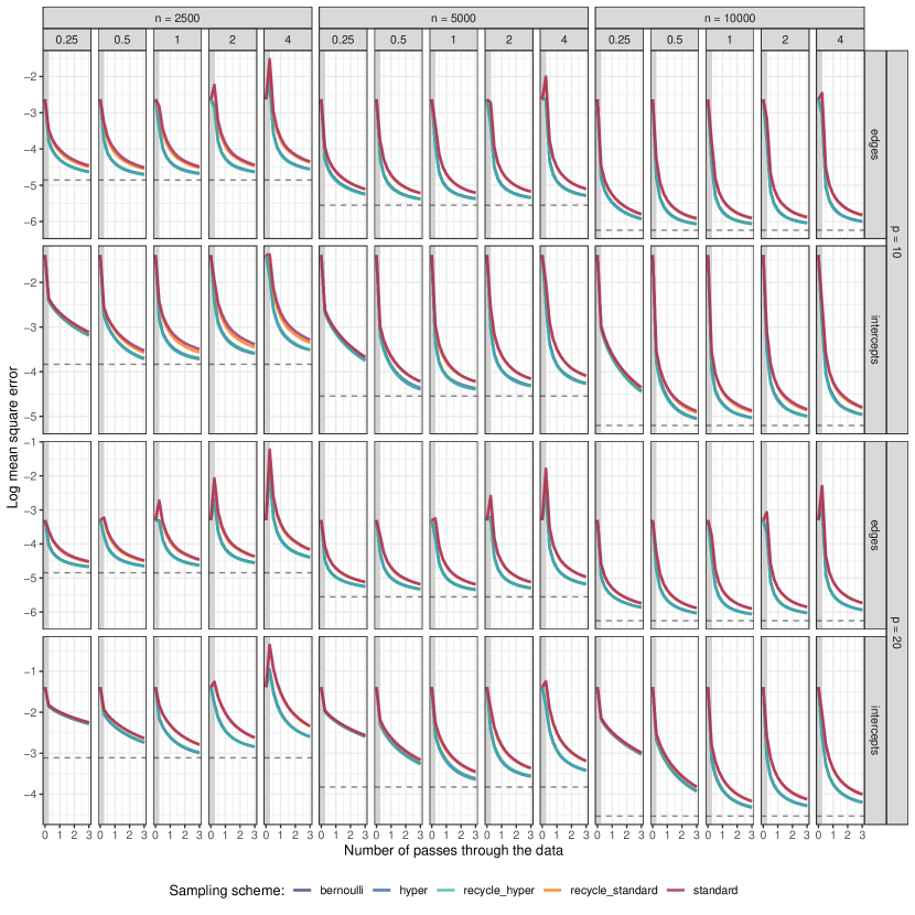
Figure 6: Ising model, $\eta_{0}\in\{0.25,0.50,1,2,4\}$. Log mean square error trajectories along the optimisation, grouped by sample size, stepsize, parameter type and number of nodes. Coloured lines refer to ${\bar{\bm{\theta}}}_{\mathcal{P}}$ under different sampling schemes, while dashed lines indicate the performance of the numerical approximation of ${\hat{\bm{\theta}}}$.

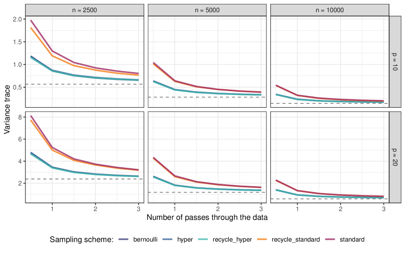
Figure 7: Ising model. Trajectories of the empirical variance trace for different $n$ and $p$. Solid lines refer to $\bar{\bm{{\bm{\theta}}}}_{\mathcal{P}}$ under different sampling schemes. Dashed lines denote the variability observed for the numerical approximation of $\hat{\bm{{\bm{\theta}}}}$.

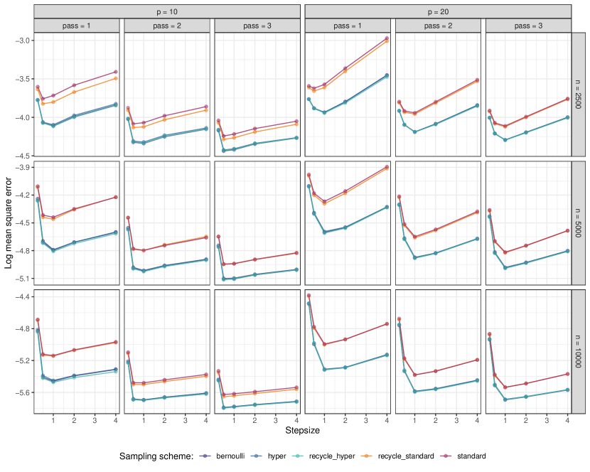
Figure 8: Ising model. Overall log mean square error as a function of the stepsize, grouped by $n$, $p$, and the number of passes through the data. Coloured lines refer to ${\bar{\bm{\theta}}}_{\mathcal{P}}$ under different sampling schemes.

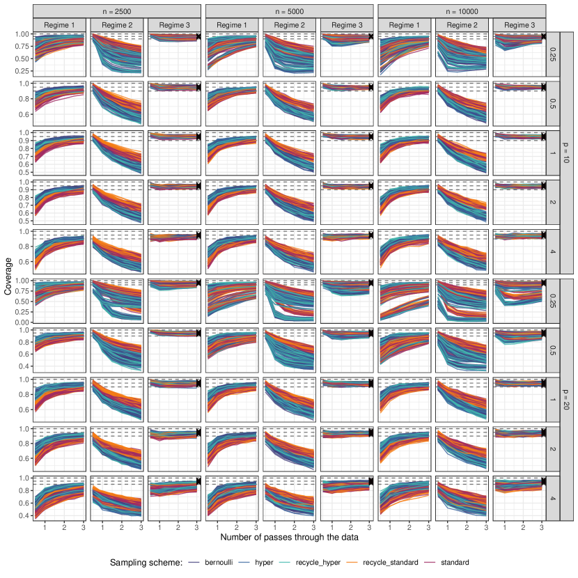
Figure 9: Ising model, $\eta_{0}\in\{0.25,0.50,1,2,4\}$. Empirical coverage of confidence intervals for ${\bar{\bm{\theta}}}_{\mathcal{P}}$ constructed according to the three asymptotic regimes in Theoem 1. Results are grouped by sample size and graph dimension. Dashed lines highlight the nominal coverage level. Coloured lines refer to scalar elements of ${\bar{\bm{\theta}}}_{\mathcal{P}}$ under different sampling schemes. Dark crosses equivalently refer to scalar elements of the numerical approximation of ${\hat{\bm{\theta}}}$.

Table 3: Comparison of computational times (s) for ${\bar{\bm{\theta}}}_{\mathcal{P}}$ with $T_{n}=3n$ under different sampling schemes and the numerical approximation of ${\hat{\bm{\theta}}}$.

$p$	$n$		bernoulli	hyper	recycle_hyper	recycle_standard	standard	numerical
$10$	2500	Total	$1.81$	$1.70$	$8.12\times 10^{-2}$	$6.66\times 10^{-2}$	$2.48\times 10^{-1}$	$2.46$
		Sampling Step	$2.33\times 10^{-4}$	$2.17\times 10^{-4}$	$2.29\times 10^{-6}$	$3.93\times 10^{-7}$	$2.46\times 10^{-5}$
		Approximation Step	$5.99\times 10^{-6}$	$6.47\times 10^{-6}$	$6.18\times 10^{-6}$	$6.11\times 10^{-6}$	$6.13\times 10^{-6}$
		Update Step	$1.65\times 10^{-7}$	$1.77\times 10^{-7}$	$1.68\times 10^{-7}$	$1.66\times 10^{-7}$	$1.62\times 10^{-7}$
	5000	Total	$7.16$	$7.48$	$2.01\times 10^{-1}$	$1.35\times 10^{-1}$	$8.03\times 10^{-1}$	$4.99$
		Sampling Step	$4.69\times 10^{-4}$	$4.89\times 10^{-4}$	$4.99\times 10^{-6}$	$5.96\times 10^{-7}$	$4.50\times 10^{-5}$
		Approximation Step	$6.21\times 10^{-6}$	$6.94\times 10^{-6}$	$6.15\times 10^{-6}$	$6.12\times 10^{-6}$	$6.18\times 10^{-6}$
		Update Step	$1.72\times 10^{-7}$	$2.09\times 10^{-7}$	$1.72\times 10^{-7}$	$1.74\times 10^{-7}$	$1.77\times 10^{-7}$
	10000	Total	$28.5$	$41.9$	$6.82\times 10^{-1}$	$2.82\times 10^{-1}$	$2.88$	$10.0$
		Sampling Step	$9.39\times 10^{-4}$	$1.39\times 10^{-3}$	$1.42\times 10^{-5}$	$1.01\times 10^{-6}$	$8.76\times 10^{-5}$
		Approximation Step	$6.61\times 10^{-6}$	$7.89\times 10^{-6}$	$6.23\times 10^{-6}$	$6.11\times 10^{-6}$	$6.26\times 10^{-6}$
		Update Step	$1.64\times 10^{-7}$	$2.10\times 10^{-7}$	$1.64\times 10^{-7}$	$1.62\times 10^{-7}$	$1.67\times 10^{-7}$
$20$	2500	Total	$3.74$	$3.90$	$2.39\times 10^{-1}$	$2.02\times 10^{-1}$	$3.84\times 10^{-1}$	$19.5$
		Sampling Step	$4.71\times 10^{-4}$	$4.87\times 10^{-4}$	$5.00\times 10^{-6}$	$4.29\times 10^{-7}$	$2.47\times 10^{-5}$
		Approximation Step	$2.40\times 10^{-5}$	$2.63\times 10^{-5}$	$2.21\times 10^{-5}$	$2.19\times 10^{-5}$	$2.19\times 10^{-5}$
		Update Step	$3.79\times 10^{-7}$	$4.28\times 10^{-7}$	$3.56\times 10^{-7}$	$3.51\times 10^{-7}$	$3.43\times 10^{-7}$
	5000	Total	$14.4$	$21.2$	$6.14\times 10^{-1}$	$3.98\times 10^{-1}$	$1.07$	$44.4$
		Sampling Step	$9.36\times 10^{-4}$	$1.38\times 10^{-3}$	$1.43\times 10^{-5}$	$6.37\times 10^{-7}$	$4.56\times 10^{-5}$
		Approximation Step	$2.20\times 10^{-5}$	$2.60\times 10^{-5}$	$2.21\times 10^{-5}$	$2.15\times 10^{-5}$	$2.16\times 10^{-5}$
		Update Step	$3.33\times 10^{-7}$	$4.28\times 10^{-7}$	$3.53\times 10^{-7}$	$3.46\times 10^{-7}$	$3.46\times 10^{-7}$
	10000	Total	$57.6$	$90.4$	$1.73$	$8.07\times 10^{-1}$	$3.40$	$98.5$
		Sampling Step	$1.89\times 10^{-3}$	$2.98\times 10^{-3}$	$3.03\times 10^{-5}$	$1.03\times 10^{-6}$	$8.69\times 10^{-5}$
		Approximation Step	$2.28\times 10^{-5}$	$2.69\times 10^{-5}$	$2.29\times 10^{-5}$	$2.15\times 10^{-5}$	$2.20\times 10^{-5}$
		Update Step	$3.30\times 10^{-7}$	$4.17\times 10^{-7}$	$3.52\times 10^{-7}$	$3.46\times 10^{-7}$	$3.52\times 10^{-7}$

C.2 Gamma frailty model

Differently to the pairwise likelihood outlined in Henderson & Shimakura (2003), we scale the objective function by $p(p-1)/2$ (i.e. the number of pairs) rather than just $p-1$. This helps to keep the same value of $\eta_{0}$ across settings with different $p$ since it assures the objective function to be comparable in magnitude across values of $p$. Implementation-wise, the parameters $\xi$ and $\rho$ are reparametrised to not introduce explicit constraints in the optimisation. In particular, we use $\check{\xi}=\exp\{\xi^{-1}\}$ and $\check{\rho}=\text{artanh}(\rho)$. In the following, we report the simulation results accounting for $n\in\{2500,5000,10000\}$, $p\in\{10,20\}$, $B=0.25n$ and $T_{n}\in\{0.5n,n,1.5n,2n,2.5n,3n\}$. Similar to previous experiments, we assess results under different choices of the stepsize, i.e. $\eta_{0}\in\{0.5,1,2,4,8\}$. As anticipated in the main simulation section, ${\mathcal{P}_{3}}$ becomes very computationally intensive when the number of likelihood components increases. For this reason, we only consider the results for recycle_hyper. However, the choice of $l=500$ in the simulation section is arbitrary, so here we report results for recycle_hyper with $l\in\{100,500,1000\}$, showing that such choice does not have noticeable impacts on the accuracy of the estimation but is crucial for the practical computational efficiency of the estimator.

Figure 10 reports the log mean square error of the stochastic estimators considered under different simulation settings. First, as anticipated at the beginning of the section, estimators based on ${\mathcal{P}_{3}}$ allow for larger stepsizes without suffering from divergence problems. Considering the reparametrisations of $\xi$ and $\rho$, in fact, recycle_standard starts experiencing diverging trajectories when $\eta_{0}>2$, while all the instances of recycle_hyper remain stable in their converging trajectories. Second, the effects of different choices of $l$ are unnoticeable. To better grasp them, we need to focus on some specific settings. Figure 11, for example, outlines the behaviour of the overall log mean square error for $\eta=2$ (the value reported in the paper). For visualisation purposes, we report only the trajectories after the burn-in period. All the lines are almost overlapping, and no clear distinction can be identified among the three instances considered. The only noticeable differences appear analysing the computational times, as reported in Table 4.

Similarly to the previous example, Figure 12 plots the overall log mean square error as a function of the stepsize. Clearly, the graphs show how methods based on ${\mathcal{P}_{3}}$ are much more stable when increasing the stepsize, while the mean square error of recycle_standard starts exploding. Figure 13 highlights the trajectories of the observed variance trace instead, showing that the mean square error differences among $\mathcal{P}_{1}$ and $\mathcal{P}_{3}$ observed in Figure 10 are due to the different variability they induce in the estimates. Trajectories are shown for $\eta_{0}=2$.

Finally, Figure 14 show the empirical coverage performance for all the possible values of $\eta_{0}$. For all the estimators considered, most difficulties arise when the stepsize is too small. In those cases, in fact, the estimates for the reparameterisations of $\xi$ and $\rho$ are still too distant from their targets. Hence, the evaluation of the empirical estimator of $\bm{H}$ and $\bm{J}$ is still not accurate enough.

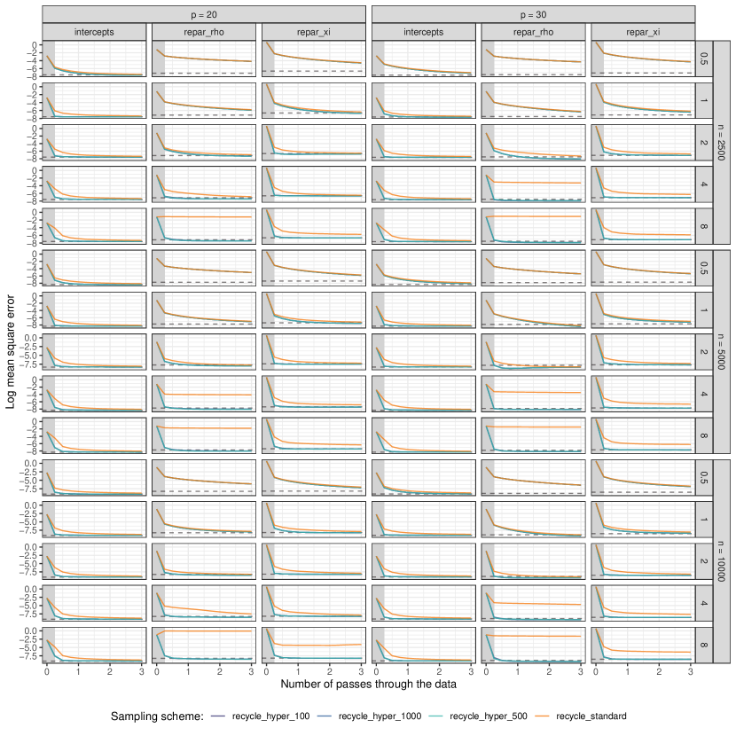
Figure 10: Gamma frailty, $\eta_{0}\in\{0.50,1,2,4,8\}$. Log mean square error trajectories along the optimisation, grouped by sample size, stepsize and parameter type. Coloured lines refer to ${\bar{\bm{\theta}}}_{\mathcal{P}}$ under different sampling schemes, while the dashed lines indicate the performance of the numerical approximation of ${\hat{\bm{\theta}}}$.

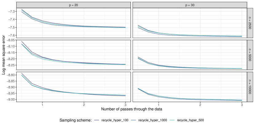
Figure 11: Gamma frailty. Overall log mean square error trajectories along the optimisation for $\eta_{0}=2$, grouped by $n$ and $p$. Coloured lines refer to the different lengths $l$ of the recycling window used for ${\mathcal{P}_{3}}$.

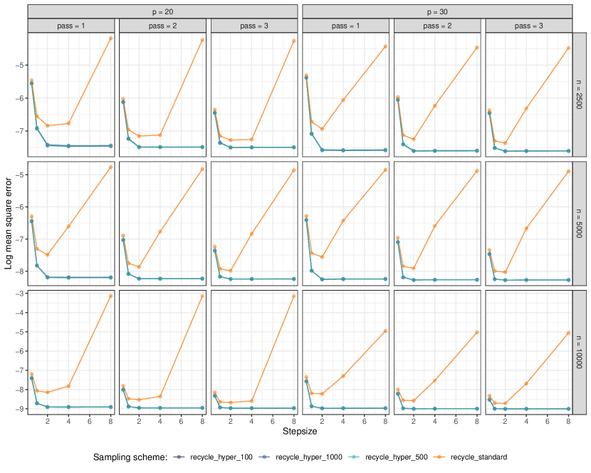
Figure 12: Gamma frailty, log mean square error as a function of the stepsize, grouped by $n$, $p$, and the number of passes through the data. Coloured lines refer to ${\bar{\bm{\theta}}}_{\mathcal{P}}$ under different sampling schemes.

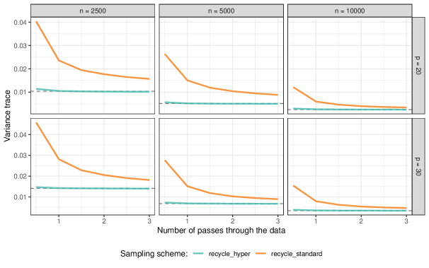
Figure 13: Gamma frailty model. Trajectories of empirical variance traces for different $n$ and $p$. Solid lines refer to $\bar{\bm{{\bm{\theta}}}}_{\mathcal{P}}$ under different sampling schemes. Dashed ones indicate values observed for the numerical approximation of $\hat{\bm{{\bm{\theta}}}}$.

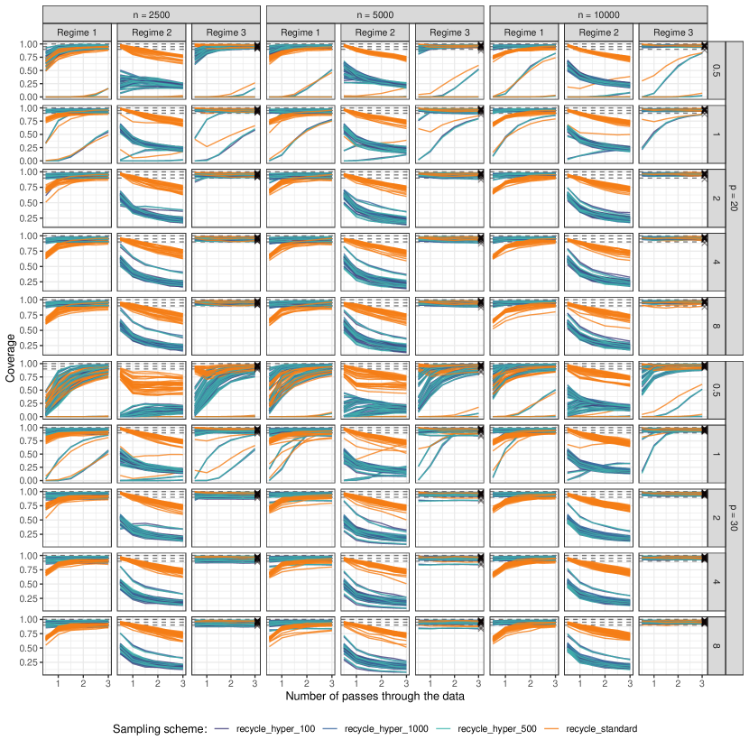
Figure 14: Gamma frailty, $\eta_{0}\in\{0.50,1,2,4,8\}$. Empirical coverage of confidence intervals for ${\bar{\bm{\theta}}}_{\mathcal{P}}$ constructed according to the three asymptotic regimes in Theoem 1. Results are grouped by sample size. Dashed lines highlight the nominal coverage level. Coloured lines refer to scalar elements of ${\bar{\bm{\theta}}}_{\mathcal{P}}$ under different sampling schemes. Dark crosses equivalently refer to scalar elements of the numerical approximation of ${\hat{\bm{\theta}}}$.

Table 4: Comparison of computational times (s) for ${\bar{\bm{\theta}}}_{\mathcal{P}}$ with $T_{n}=3n$ under different sampling schemes and the numerical approximation of ${\hat{\bm{\theta}}}$.

$p$	$n$	operation	recycle_hyper_100	recycle_hyper_1000	recycle_hyper_500	recycle_standard	numerical
20	2500	Total	$1.62$	$1.22$	$1.25$	$8.93\times 10^{-1}$	$6.76$
		Sampling Step	$1.57\times 10^{-6}$	$1.60\times 10^{-6}$	$1.55\times 10^{-6}$	$4.07\times 10^{-7}$
		Approximation Step	$1.52\times 10^{-4}$	$1.54\times 10^{-4}$	$1.53\times 10^{-4}$	$1.17\times 10^{-4}$
		Update Step	$1.31\times 10^{-6}$	$1.31\times 10^{-6}$	$1.31\times 10^{-6}$	$1.17\times 10^{-7}$
	5000	Total	$4.66$	$2.61$	$2.77$	$1.80$	$13.5$
		Sampling Step	$1.60\times 10^{-6}$	$1.68\times 10^{-6}$	$1.59\times 10^{-6}$	$4.29\times 10^{-7}$
		Approximation Step	$1.55\times 10^{-4}$	$1.58\times 10^{-4}$	$1.55\times 10^{-4}$	$1.18\times 10^{-4}$
		Update Step	$1.31\times 10^{-6}$	$1.32\times 10^{-6}$	$1.31\times 10^{-6}$	$1.20\times 10^{-7}$
	10000	Total	$18.1$	$6.32$	$7.24$	$3.64$	$27.2$
		Sampling Step	$1.68\times 10^{-6}$	$1.68\times 10^{-6}$	$1.62\times 10^{-6}$	$4.48\times 10^{-7}$
		Approximation Step	$1.64\times 10^{-4}$	$1.64\times 10^{-4}$	$1.59\times 10^{-4}$	$1.19\times 10^{-4}$
		Update Step	$1.32\times 10^{-6}$	$1.31\times 10^{-6}$	$1.31\times 10^{-6}$	$1.20\times 10^{-7}$
30	2500	Total	$4.23$	$2.95$	$3.03$	$2.23$	$12.0$
		Sampling Step	$1.86\times 10^{-6}$	$1.85\times 10^{-6}$	$1.81\times 10^{-6}$	$7.45\times 10^{-7}$
		Approximation Step	$3.74\times 10^{-4}$	$3.72\times 10^{-4}$	$3.68\times 10^{-4}$	$2.94\times 10^{-4}$
		Update Step	$1.35\times 10^{-6}$	$1.34\times 10^{-6}$	$1.33\times 10^{-6}$	$1.31\times 10^{-7}$
	5000	Total	$13.8$	$6.31$	$7.09$	$4.45$	$24.4$
		Sampling Step	$2.00\times 10^{-6}$	$1.83\times 10^{-6}$	$1.88\times 10^{-6}$	$8.03\times 10^{-7}$
		Approximation Step	$3.94\times 10^{-4}$	$3.73\times 10^{-4}$	$3.77\times 10^{-4}$	$2.94\times 10^{-4}$
		Update Step	$1.35\times 10^{-6}$	$1.33\times 10^{-6}$	$1.33\times 10^{-6}$	$1.31\times 10^{-7}$
	10000	Total	$54.0$	$15.4$	$19.3$	$8.88$	$48.1$
		Sampling Step	$2.03\times 10^{-6}$	$1.86\times 10^{-6}$	$1.88\times 10^{-6}$	$8.00\times 10^{-7}$
		Approximation Step	$4.02\times 10^{-4}$	$3.86\times 10^{-4}$	$3.88\times 10^{-4}$	$2.93\times 10^{-4}$
		Update Step	$1.35\times 10^{-6}$	$1.33\times 10^{-6}$	$1.34\times 10^{-6}$	$1.32\times 10^{-7}$

Appendix D Supplementary material NESARC data

A description of the $p=32$ items considered can be found in Table LABEL:tab:dict. As described in Section 5, the optimisation stops by controlling the holdout average composite log-likelihood. Panel (A) in Figure 15 shows the estimated edge parameters along the optimization. The stable behavior of most of their trajectories suggests a decreasing utility of additional iterations. Panel (B) instead tracks the holdout negative composite log-likelihood, which exhibits a sharp drop at the beginning of the optimization and then slowly decreases until the procedure ends at $T_{n}$. Thus, while the algorithm does not strictly minimise the holdout objective function, the decreasing trajectory suggests it is avoiding overfitting.

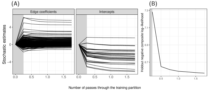
Figure 15: (A) Trajectories of the estimated parameters. (B) Average negative log-likelihood on the holdout partition. Grey areas denote the burn-in period.

Since the original NESARC data is not publicly available anymore, the analysis carried out in Section 5 can be reproduced on synthetic data. In particular, we provide a dataset simulated from the Ising model with parameters given by the numerical estimates of $\hat{\bm{\theta}}$ computed on the original NESARC data. Figure 16 shows how the stochastic estimates for the edges of the Ising model computed on the simulated dataset compare with the parameters generating the data and with the stochastic estimates computed on the original NESARC answers. While not identical, the results are still very similar and can be used as a reference for reproducing the analysis.

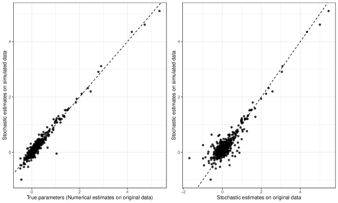
Figure 16: Comparing estimated edges on the simulated dataset against numerical and stochastic estimates on original data.

Table 5: Description of the items of the NESARC survey considered in the analysis.

Item	Area	Description
S4AQ1	Low mood	ever had 2-week period when felt sad, blue, depressed, or down most of time
S4AQ2	Low mood	ever had 2-week period when didn’t care about things usually cared about
S4BQ1	Low mood	blood/natural father ever depressed
S4BQ2	Low mood	blood/natural mother ever depressed
S4CQ1	Low mood	had 2+ years period when mood was low, sad or depressed most of day, more than half the time
S5Q1	High mood	had 1+ week period of excitement/elation that seemed not normal self
S5Q2	High mood	had 1+ week period of excitement/elation that made others concerned about you
S5Q3	High mood	had 1+ week period irritable/easily annoyed that caused you to shout/break things/start fights or arguments
S6Q1	Panic disorders	had panic attack, suddenly felt frightened/overwhelmed/nervous as if in great danger but were not
S6Q2	Panic disorders	was surprised by panic attack that happened out of the blue, for no real reason or in a situation where didn’t expect to be frightened/nervous
S6Q3	Panic disorders	thought was having heart attack, but doctor said just nerves or panic attack
S7Q1	Social phobia	ever had strong fear or avoidance of social situation
S7Q2	Social phobia	had fear/avoidance of social situation due to fear of embarrassment at what you might say/do around others
S7Q3	Social phobia	had fear/avoidance of social situation due to fear of becoming speechless, having nothing to say or saying something foolish
S8Q1A1	Specific phobia	ever had fear/avoidance of insects, snakes, birds, other animals
S8Q1A2	Specific phobia	ever had fear/avoidance of heights
S8Q1A5	Specific phobia	ever had fear/avoidance of flying
S8Q1A7	Specific phobia	ever had fear/avoidance of being in closed spaces
S8Q1A8	Specific phobia	ever had fear/avoidance of seeing blood/getting an injection
S9Q1B	General anxiety	ever had 6+ month period felt very tense/nervous/worrie most of time abouteveryday problems
S10Q1A1	Personality disorders	avoid jobs or tasks that deal with a lot of people
S10Q1A2	Personality disorders	avoid getting involved with people unless certain they will like you
S10Q1A3	Personality disorders	find it hard to be ’open’ even with people you are close to
S10Q1A4	Personality disorders	often worry about being criticized or rejected in social situations
S10Q1A5	Personality disorders	believe that you are not as good, as smart, or as attractive as most people
S10Q1A7	Personality disorders	afraid of trying new things or doing things outside usual routine because afraid of being embarrassed
S11AQ1A1	Antisocial disorders	often cut class, not go to class or go to school and leave without permission
S11AQ1A2	Antisocial disorders	ever stay out late at night even though parents told you to stay home
S11AQ1A3	Antisocial disorders	ever have time when bullied or pushed people around or tried to make them afraid of you
S11AQ1A4	Antisocial disorders	ever run away from home at least twice or run away and stay away for a longer time
S11AQ1A6	Antisocial disorders	more than once quit a job without knowing where would find another one
S11AQ1A9	Antisocial disorders	ever have time lasting 1+ months when had no regular place to live

References

- (1)
- Atchadé et al. (2017) Atchadé, Y. F., Fort, G. & Moulines, E. (2017), ‘On perturbed proximal gradient algorithms’, The Journal of Machine Learning Research 18(1), 310–342.
- Bellio & Varin (2005) Bellio, R. & Varin, C. (2005), ‘A pairwise likelihood approach to generalized linear models with crossed random effects’, Statistical Modelling 5(3), 217–227.
- Besag (1974) Besag, J. (1974), ‘Spatial interaction and the statistical analysis of lattice systems’, Journal of the Royal Statistical Society: Series B (Methodological) 36(2), 192–225.
- Blum et al. (1958) Blum, J. R., Chernoff, H., Rosenblatt, M. & Teicher, H. (1958), ‘Central limit theorems for interchangeable processes’, Canadian Journal of Mathematics 10, 222–229.
- Bordes et al. (2009) Bordes, A., Bottou, L. & Gallinari, P. (2009), ‘SGD-QN: Careful quasi-Newton stochastic gradient descent’, Journal of Machine Learning Research 10, 1737–1754.
- Borsboom (2022) Borsboom, D. (2022), ‘Possible futures for network psychometrics’, Psychometrika 87(1), 253–265.
- Byrd et al. (2011) Byrd, R. H., Chin, G. M., Neveitt, W. & Nocedal, J. (2011), ‘On the use of stochastic hessian information in optimization methods for machine learning’, SIAM Journal on Optimization 21(3), 977–995.
- Byrd et al. (2016) Byrd, R. H., Hansen, S. L., Nocedal, J. & Singer, Y. (2016), ‘A stochastic quasi-Newton method for large-scale optimization’, SIAM Journal on Optimization 26(2), 1008–1031.
- Chen et al. (2020) Chen, X., Lee, J. D., Tong, X. T. & Zhang, Y. (2020), ‘Statistical inference for model parameters in stochastic gradient descent’, The Annals of Statistics 48(1), 251 – 273.
-
DeBruine (2021)
DeBruine, Z. (2021), RcppClock: Seamless ’Rcpp’ Benchmarking.
R package version 1.1.
https://CRAN.R-project.org/package=RcppClock - Eddelbuettel & François (2011) Eddelbuettel, D. & François, R. (2011), ‘Rcpp: Seamless R and C++ integration’, Journal of Statistical Software 40(8), 1–18.
-
Epskamp (2014)
Epskamp, S. (2014), IsingSampler: Sampling methods and distribution functions for the Ising model.
R package version 0.1.1.
https://cran.r-project.org/web/packages/IsingSampler - Epskamp et al. (2018) Epskamp, S., Borsboom, D. & Fried, E. I. (2018), ‘Estimating psychological networks and their accuracy: A tutorial paper’, Behavior Research Methods 50(1), 195–212.
- Grant et al. (2003) Grant, B. F., Moore, T., Shepard, J. & Kaplan, K. (2003), ‘Source and accuracy statement: Wave 1 national epidemiologic survey on alcohol and related conditions (nesarc)’, Bethesda, MD: National Institute on Alcohol Abuse and Alcoholism 52.
- Han et al. (2021) Han, R., Luo, L., Lin, Y. & Huang, J. (2021), ‘Online inference with debiased stochastic gradient descent’, Biometrika . To appear.
- Henderson & Shimakura (2003) Henderson, R. & Shimakura, S. (2003), ‘A serially correlated gamma frailty model for longitudinal count data’, Biometrika 90(2), 355–366.
- Holm (1979) Holm, S. (1979), ‘A simple sequentially rejective multiple test procedure’, Scandinavian Journal of Statistics 6(2), 65–70.
- Ising (1924) Ising, E. (1924), Beitrag zur theorie des ferro-und paramagnetismus, PhD thesis, Grefe & Tiedemann Hamburg.
- Janková & van de Geer (2018) Janková, J. & van de Geer, S. (2018), Inference in high-dimensional graphical models, in ‘Handbook of Graphical Models’, CRC Press, pp. 325–350.
- Katsikatsou et al. (2012) Katsikatsou, M., Moustaki, I., Yang-Wallentin, F. & Jöreskog, K. G. (2012), ‘Pairwise likelihood estimation for factor analysis models with ordinal data’, Computational Statistics & Data Analysis 56(12), 4243–4258.
- Lee & Hastie (2015) Lee, J. D. & Hastie, T. J. (2015), ‘Learning the structure of mixed graphical models’, Journal of Computational and Graphical Statistics 24(1), 230–253.
- Lindsay (1988) Lindsay, B. G. (1988), ‘Composite likelihood methods’, Contemporary Mathematics 80(1), 221–239.
- Luo et al. (2021) Luo, L., Han, R., Lin, Y. & Huang, J. (2021), ‘Statistical inference in high-dimensional generalized linear models with streaming data’, arXiv:2108.04437 .
- Nielsen (2000) Nielsen, H. B. (2000), ucminf: An algorithm for unconstrained, nonlinear optimization, Technical report, IMM, Department of Mathematical Modelling, Technical University of Denmark.
- Pinelis (2015) Pinelis, I. (2015), ‘Relationships between the first four moments’, The American Mathematical Monthly 122(5), pp. 479–481.
- Polyak (1987) Polyak, B. T. (1987), Introduction to Optimization, Optimization Software, Inc., Publications Division.
- Polyak & Juditsky (1992) Polyak, B. T. & Juditsky, A. B. (1992), ‘Acceleration of stochastic approximation by averaging’, SIAM Journal on Control and Optimization 30(4), 838–855.
- Robbins & Monro (1951) Robbins, H. & Monro, S. (1951), ‘A stochastic approximation method’, The Annals of Mathematical Statistics 22(3), 400–407.
- Ruppert (1988) Ruppert, D. (1988), Efficient estimations from a slowly convergent Robbins-Monro process, Technical report, Cornell University Operations Research and Industrial Engineering.
- Toulis & Airoldi (2017) Toulis, P. & Airoldi, E. M. (2017), ‘Asymptotic and finite-sample properties of estimators based on stochastic gradients’, The Annals of Statistics 45(4), 1694–1727. Publisher: Institute of Mathematical Statistics.
- Varin et al. (2011) Varin, C., Reid, N. & Firth, D. (2011), ‘An overview of composite likelihood methods’, Statistica Sinica 21(1), 5–42.
- Varin & Vidoni (2005) Varin, C. & Vidoni, P. (2005), ‘A note on composite likelihood inference and model selection’, Biometrika 92(3), 519–528.
- White (1982) White, H. (1982), ‘Maximum likelihood estimation of misspecified models’, Econometrica 50(1), 1–25.
- Zhang & Chen (2022) Zhang, S. & Chen, Y. (2022), ‘Computation for latent variable model estimation: A unified stochastic proximal framework’, Psychometrika 87(4), 1473–1502.
- Zhang & Chen (2023) Zhang, S. & Chen, Y. (2023), ‘A note on Ising network analysis with missing data’, arXiv:2307.00567 .