Amortized Network Intervention to Steer the Excitatory Point Processes

Abstract

We tackle the challenge of large-scale network intervention for guiding excitatory point processes, such as infectious disease spread or traffic congestion control. Our model-based reinforcement learning utilizes neural ODEs to capture how the networked excitatory point processes will evolve subject to the time-varying changes in network topology. Our approach incorporates Gradient-Descent based Model Predictive Control (GD-MPC), offering policy flexibility to accommodate prior knowledge and constraints. To address the intricacies of planning and overcome the high dimensionality inherent to such decision-making problems, we design an Amortize Network Interventions (ANI) framework, allowing for the pooling of optimal policies from history and other contexts, while ensuring a permutation equivalent property. This property enables efficient knowledge transfer and sharing across diverse contexts. Our approach has broad applications, from curbing infectious disease spread to reducing carbon emissions through traffic light optimization, and thus has the potential to address critical societal and environmental challenges.

1 Introduction

In the face of widespread epidemic outbreaks, governments must act swiftly and wisely to control the spread of diseases, often through measures like temporary city lockdowns or travel restrictions (Salathé & Jones, 2010; Sambaturu et al., 2020). Similarly, optimizing traffic light schedules in densely populated urban areas is essential to alleviate traffic congestion. These real-world scenarios highlight the necessity of guiding event processes across networks by modifying network structures as needed.

The dynamics of these networked events are complex, involving vast volumes of data across multiple dimensions. Decision-making must be reliable and adaptable to rapidly changing circumstances. However, altering dynamic network structures presents a computational challenge, especially in scenarios like city traffic control, where real-world constraints and various factors must be considered. For instance, when regulating the coronavirus, government interventions must balance health concerns with economic implications and public sentiment. Thus, this network intervention problem requires innovative solutions.

We model events, such as infectious disease spread or traffic congestion, as multivariate excitatory temporal point processes. Our goal is to solve a model-based reinforcement learning (MBRL) problem: guiding large-scale excitatory processes across dynamic networks by modifying network structures to minimize costs. This presents challenges in both modeling and computation.

First, modeling networked excitatory point processes with complex excitation patterns is challenging. Traditional disease models, such as SIR models (Weiss, 2013), use ordinary differential equations (ODEs). These models divide the population into compartments like susceptible, infectious, and recovered, utilizing ODEs to capture changes over time. Similarly, classic traffic flow models rely on ODEs or PDEs. For example, the Lighthill-Whitham-Richards (LWR) model (Lighthill & Whitham, 1955; Richards, 1956) employs PDEs to describe traffic density evolution along roads. These models offer simplified yet insightful representations of disease dynamics and traffic patterns. To address the complex dynamics of high-dimensional event sequences, we turn to the Neural ODE model (Chen et al., 2018), a data-driven approach for modeling ODE dynamics. Importantly, our model-based RL framework can adapt to various event process models beyond Neural ODEs, allowing for efficient computational choices while maintaining high prediction accuracy.

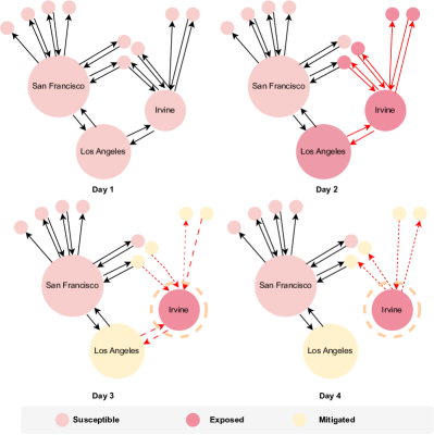
Figure 1: A viral infection started in a random region, with a network intervention curbing its spread. Nodes represent counties, and edges are roads. On day two, one county had a spike in cases, which spread to its neighboring county (red node). On days three and four, external lockdowns were alternated on neighboring roads to curb the pandemic (yellow node).

The second challenge is to design intervention policies that accommodate domain constraints, incorporate feedback rapidly, and adapt to changing circumstances. Gradient-Descent-based Model Predictive Control (GD-MPC) with medium-sized neural network models (Nagabandi et al., 2018; Bharadhwaj et al., 2020) is a valuable approach among Model-based Reinforcement Learning (MBRL) algorithms. MPC solves a finite-horizon optimization problem at each time step using a sliding window approach, which improves decision-making. MPC advantages include explicit consideration of system dynamics and constraints, continuous adaptation based on feedback, and flexibility in incorporating various objectives and constraints. These features make MPC a powerful tool for designing adaptive intervention policies for complex, high-frequency event sequences.

The third challenge is scaling the MBRL algorithm for high-dimensional problems, like controlling an entire city’s traffic network. We’ve developed the Amortize Network Interventions (ANI) framework to tackle this issue. ANI enables us to extract optimal policies from historical data and similar tasks while preserving a crucial permutation equivalent property. We introduce a novel metric to aid in learning permutation equivalent representations, ensuring efficient parameter transfer and sharing across tasks, thereby enhancing our approach’s adaptability and scalability.

Our proposed method is strategically crafted to meet the above three challenges. To assess its efficacy and efficiency, we have conducted comprehensive experiments using synthetic traffic congestion data and real-world COVID datasets. The experimental results demonstrate the effectiveness of our approach in adeptly steering excitatory point processes through the control of network dynamics.

2 Problem Formulation: Model-based RL

We begin by modeling spatial-temporal event sequences as temporal graph networks. For infectious diseases, we divide the geographical map into regions, each corresponding to a graph node. Each time step records new confirmed cases in these regions, creating a discrete-time dynamic graph. In the case of traffic congestion incidents, we use a lane-based approach. Each lane on a road becomes a network node, and at each time step, we track the congestion count for each lane within the specified time interval.

Formally, we define a temporal graph network $\mathcal{G}_{t}=(\mathcal{V}_{t},\mathcal{E}_{t})$ indexed by $t=0,1,\dots$, with $\mathcal{V}_{t}$ and $\mathcal{E}_{t}$ representing the node and edge sets at time $t$. The network maintains a fixed set of $N$ nodes at each time step. For each node, representing either a region or a traffic lane, we observe a sequence of event spike counts at each time step. This results in a spike count matrix observed up to time $t$, denoted as $\mathbf{X}_{t}\in\mathbb{N}^{t\times N}$. Here, $\mathbf{X}_{t}$ contains $N$ time-series of event counts: $\mathbf{X}_{t}=\{\mathbf{x}^{t}_{1},\dots,\mathbf{x}^{t}_{N}\}$.

We focus on the problem of managing the flow of the event counts to achieve specific levels at minimal cost, through sequential adjustment of the edge $\{\mathcal{E}_{t}\}_{t\geq 0}$. Adding or removing certain edges will alter the connections between corresponding nodes, influencing the generative patterns of events. This formulation has broad applications, including containing epidemic outbreaks through lockdown policies or regulating traffic congestion by strategically designing traffic lights.

We consider a finite-time horizon control framework, where an agent aims to find an edge intervention policy $\pi(\mathbf{h}^{t}):\mathcal{S}\to\mathcal{A}$, given the current state $\mathbf{h}^{t}$, such that the cumulative expected reward within a fixed time horizon is maximized,

$$\pi^{*}=\arg\,\max_{\pi\in\Pi}\,\,\mathbb{E}\left[\sum_{t=0}^{T}r^{t}(\mathbf{h}^{t},\mathbf{a}^{t})\right],$$ (1)

where $\mathbf{h}^{0}\sim p^{0}(\cdot)$, $\mathbf{h}^{t+1}\sim\mathbb{P}(\cdot|\mathbf{h}^{t},\mathbf{a}^{t})$, and $\mathbf{a}^{t}\sim\pi(\mathbf{h}^{t})$. Several key aspects are as follows:

1. Environment: high-dimensional event sequences $\{\mathbf{X}_{t}\}_{t\geq 0}$ with stationary dynamics, occurring over a temporal graph network $\{\mathcal{G}_{t}=(\mathcal{V}_{t},\mathcal{E}_{t})\}_{t\geq 0}$.

2. State: all the historical observations up to current time $t$, including event sequence and intervention histories. We assume the state information is completely encoded into a graph embedding vector $\mathbf{h}^{t}$, where $\mathbf{h}^{t}\in\mathbb{R}^{N\times D}$ and $D$ is the embedded dimension. We will explain how to perform the state embedding when we describe our predictive model for the event sequences.

3. Action: the action space is defined as $\mathcal{A}:=\{\mathbf{a}\in\{0,1\}^{N\times N}|\mathbf{a}^{T}\mathbf{c}\leq B,\sum_{m,n}\mathbf{a}_{mn}\leq K\}$, where $\mathbf{c}$ is the intervention cost to the edges, $B\in\mathbb{R}_{+}$ is the total budget at each stage, and $K$ is the maximum number of edges to be intervened at each stage. Here, we put some budget constraints on the action space to enable a safe policy.

4. State Transition: although the dynamics of the event sequences are unknown, we will build a predictive model $\mathbb{P}_{\theta}(\cdot|\mathbf{h}^{t},\mathbf{a}^{t})$ and estimate the model parameters $\theta$ using observational data.

5. Reward Function: the reward function is tailored to suit particular applications. It is influenced by cumulative event counts and can be augmented by incorporating other societal or environmental considerations. Note that our time-dependent reward function $r^{t}$ can entail a discount factor $\gamma^{t}$.

Since the state transition model $\mathbb{P}_{\theta}(\cdot|\mathbf{h},\mathbf{a})$ are unknown, we need to learn them from data. The optimal policy $\pi^{*}$ in Eq. (1) can be estimated by repeated querying the model. In the next section, we will explain how to build the predictive model for the environment, e.g., the event sequence model. It is noteworthy to mention that solving a large-scale problem requires solving the abovementioned problem (Eq. (1)) repeatedly – from one region to multiple regions, from one fixed time window to multiple time windows. How to leverage the optimal policies of previous subproblems to ease the optimization of a new one? In this paper, we have devised the Amortized Network Interventions (ANI) framework. As demonstrated in Fig. 2, ANI enables us to aggregate optimal policies from historical data and similar tasks while preserving a critical permutation equivalent property. We will elaborate on ANI in Section 5.

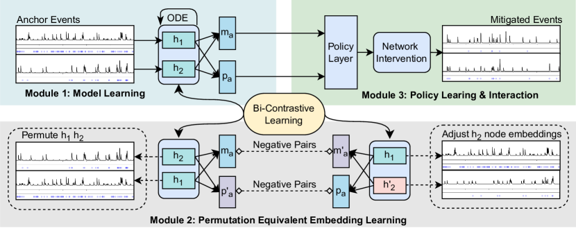
Figure 2: Overview of the Method. The proposed Amortized Network Intervention contains three modules. The first module is to generate a latent node embedding $\mathbf{h}_{n}^{i}$ and evolve the latent states through the NJODE model. The second module learns a Permutation Equivalent Embedding (PEE) over the latent space $\mathbf{h}_{n}$ by a bi-contrastive loss function prepared for the downstream adaptation. The third module accesses the learned PEE from the second module and generates a permutation equivalent policy via Model Predictive Control (MPC).

3 Modeling the Environment: Networked Jump ODE Model

Inspired by traditional ODE- and PDE-based models in infectious disease and traffic flow studies, we propose a data-driven approach to model event sequence dynamics. We introduce a Networked Jump ODE (NJODE) model to replicate the evolution of excitatory point processes, drawing from concepts in Neural Spatio-Temporal Point Processes (Chen et al., 2020a) and Neural Jump SDEs (Jia & Benson, 2019), which have been used for fine-grained spatio-temporal event process modeling. We modify these models to handle large event counts in discrete-time and high-frequency scenarios. We model the excitatory point processes based on two assumptions. (1) Processes with the same network share triggering kernel model parameters but have distinct parameters for emission probability distributions. This scalability helps accommodate more nodes in local regions without significantly increasing model parameters. (2) Different local regions share a similar underlying dynamic structure. This enables fine-tuning or reusing pre-trained local region dynamics for unseen local region dynamics.

Evolution of latent states We formalize the state transition model by an ODE system with jumps, where the latent state $\mathbf{h}^{t}$ at each time $t$ evolves according to

$$\mathbf{h}_{n}^{t_{0}} =\mathbf{h}_{n}^{0}$$ (2)

$$\frac{d\mathbf{h}^{t}_{n}}{dt} =f_{h}(t,\mathbf{h}^{t}_{n}),\ \ \forall t\in\mathbb{R}_{+}\setminus\cup_{i}\{t_{i}\},$$ (3)

$$\lim_{\epsilon\downarrow 0}\mathbf{h}_{n}^{t_{i}+\epsilon} =\textstyle\sum_{m\in\mathcal{N}_{n}}w_{m\to n}\cdot\phi_{h}(\mathbf{h}_{m}^{t_{i}},x_{m}^{t_{i}}).$$ (4)

Here, $\mathcal{N}_{n}$ is the neighbors of node $n$ and $\mathbf{h}_{n}^{t_{i}}\in\mathbb{R}^{D}$ is the latent state for node $n$, where $n\in\{1,2,\dots,N\}$. $t_{i}$ represents the time stamp to record discrete jumps. Rather than treating the event arrival time as a random variable (Chen et al., 2020a), we regard the total number of discrete events with interval $[t_{i-1},t_{i})$ as a random variable $x^{t_{i}}$, allowing us to process high-frequency temporal data like traffic flow. The use of $\epsilon$ is to portray $\mathbf{h}^{t}_{n}$ as a left-continuous function with right limits at any fixed $t_{i}$. $f_{h}$ is used to model the continuous change and $\phi_{h}$ is used to model the instantaneous jump based on neighbors’ events $x^{t_{i}}_{m}$. $f_{h}$ and $\phi_{h}$ are shared for different event processes in the same local region. $w_{m\to n}$ indicates the influence strength from node $m$ to $n$.We denote $\mathbf{W}=[w_{m\to n}]$ as the influence matrix. This architecture is similar to a recurrent neural network with a continuous-time latent state modeled by a neural ODE. Under this formulation, the latent state $\mathbf{h}^{t}_{n}$ incorporates both historical information from itself and abrupt changes triggered by neighboring nodes. This mechanism for preserving abrupt change and recording memory is important to model excitatory point processes and generalize other unseen dynamics.

Conditional emission probability distribution At each time $t_{i}$, we parameterize the event count distribution as a function of the latent state $\mathbf{h}^{t}$. Specifically, in the rest of the paper, we assume the spike count $x^{t}_{n}$ follows a Poisson distribution, whose intensity $\lambda_{n}^{t}$ is a function of $\mathbf{h}_{n}^{t}$:

$$\lambda_{n}^{t}=\text{exp}(b_{\psi_{n}}+g_{\psi}(\mathbf{h}_{n}^{t})).$$ (5)

Here, we assume $g_{\psi}$ is the shared distribution parameter neural network among different nodes, while $b_{\psi_{n}}$ is the distinct baseline variable for different nodes. Given this model, we see that the final emission probability of $x^{t}_{n}$ conditioned on historical observations $x^{<t}_{n}$ is given by

$$\log p_{\theta}(x^{t}_{n}|x^{<t}_{n})=-\lambda_{n}^{t}+x^{t}_{n}\log\lambda^{t}_{n}-\log(x^{t}_{n}!)$$ (6)

where $\theta$ refers to all model parameters. Finally, given a spike counts matrix $\mathbf{X}\in\mathbb{N}^{N\times T}$, we assume different nodes at different times are conditionally independent given the latent state $\mathbf{h}^{t}$, thereby we estimate the parameter $\theta$ by maximum log-likelihood and the total log-likelihood is expressed as

$$\mathcal{L}_{LLH}(\mathbf{X};\theta)=\sum_{t=0}^{T-1}\sum_{n=1}^{N}\log p_{\theta}(x^{t}_{n}|x^{<t}_{n}).$$ (7)

Mean field approximation for reward modeling In our MBRL formulation, we use the estimated event process model as our environment simulator to perform online planning. The reward is usually a function of the generated future events. For example, it can be the negative value of the total number of newly infested people at the next stage, i.e., $r^{t}_{n}:=-\sum_{n=1}^{N}\hat{x}^{t+1}_{n}$, where $\hat{x}_{n}^{t}$ denotes an estimator of $x_{n}^{t}$. In the planning phase, accurately approximating the expected cumulative reward demands a considerable number of rollouts from conditional emission probability distributions, which can be time-consuming. Instead, we construct a reward model $r^{t}_{n,\text{MFA}}$ based on the mean field approximation (MFA) for $x^{t}_{n}$ by averaging over the high dimensional freedoms on the conditional term (detailed in Appendix E). As a result, during planning, we have a deterministic reward model after removing the stochasticity in Eq. (4) and replacing $x_{m}^{t_{i}}$ with its mean. This mean field approximation enables efficient online planning.

4 Gradient-Descen-based Model Predictive Control

Given the estimated environment model in Section 3, we design control algorithms to obtain an optimal event flow steering policy by performing interventions to the graph’s edges. Specifically, for an $N$-node influence graph, each action involves selecting a subset of $k$ ($k\leq K$) edges from $N(N-1)$ direct edges (excluding self-connections). Hence, we can represent action $\mathbf{a}^{t}$ as a $k$-hot matrix, resulting in the intervened influence graph given by $\mathbf{W}\odot(1-\mathbf{a}^{t})$. Our approach draws inspiration from Adaptive MPC (Garcia et al., 1989), which dynamically adjusts and enhances a model in real-time to account for time-varying dynamic characteristics. We construct a policy-gradient-based control algorithm and incorporate flexible constraints on the action space.

Receding Horizon Control We construct our cumulative objective function from a rolling-horizon perspective. At each time $t$, we optimize the policy $\pi_{\varphi}$ by looking $T$-step ahead, i.e.,

$$\pi^{*}_{\varphi}=\operatorname*{arg\,max}_{\pi_{\varphi}}\sum_{i=0}^{T-1}r^{t}_{\textrm{MFA}}(\mathbf{h}^{t+i},\pi_{\varphi}(\mathbf{h}^{t+i}),f_{h}\circ\phi_{h}(\mathbf{h}^{t+i},\pi_{\varphi}(\mathbf{h}^{t+i})),$$ (8)

where the expected reward is replaced by the MFA, and the function composition $f_{h}\circ\phi_{h}$ will give the next state. In online planning, the learned model is used to explore state trajectories that start from the current latent state $\mathbf{h}^{t}$. After finding a reward-maximizing policy from time $t$ to $t+T$, only the first action is employed. At time $t+1$, when new data arrives, a new latent state $\mathbf{h}^{t+1}$ is queried again from our model, and the calculations repeat, yielding a new policy and prediction trajectory.

Gradient-Descent-based Optimization Instead of exhaustively searching the discrete combinatorial action space to optimize our objective, we approximate this space using a continuous relaxation technique (Xie & Ermon, 2019). We replace $\mathbf{W}\odot(1-\mathbf{a}^{t})$ with $\mathbf{W}\odot(1-\mathbf{p}^{t})$, where $\mathbf{p}^{t}$ represents edge selection probabilities. With this reparametrization, the objective becomes a fully deterministic function of the policy and dynamics, enabling end-to-end differentiable policy learning.

Incorporating Fairness Constraints and More We can incorporate flexible constraints, including fairness, into the decision-making process. We distinguish between hard and soft constraints in our approach. For hard constraints, such as limitations on consecutive lockdown days for a county (e.g., not locking down a county for more than certain consecutive days), we can employ a dynamic mask to explicitly exclude actions that fall outside the feasible space. As for soft constraints, like ensuring overall fairness in the policy, we can design an additional reward term, denoted as $r^{t}_{\text{aug}}$, and scale it by $\lambda$. This augmented reward term is jointly updated with the policy to enforce fairness within the optimization objective.

5 Making Large-Scale Problem Tractable: Amortized Policy

Input: Task pools $\mathcal{B}$ and a pretrained model pool $\Theta$ learned based on Eq. (7)

Result: Policy parameters $\varphi$ and representation parameters $\psi$

Initialize parameters $\varphi$ and $\psi$;

while meta-training not complete do

       Sample a network $\mathcal{M}_{i}\sim\mathcal{B}$ and corresponding model $\theta_{i}\in\Theta$;

       // Policy & Representation Learning

       Optimize $\{\varphi,\psi\}$ jointly based on Eq. (8)(11);

       Obtain intervened network $\mathbf{W}^{\prime}$ based on policy $\pi_{\varphi}$;

       // Planning ahead

       Collect new data $\mathcal{D}_{i}$ by NJODESolver($\mathbf{W}^{\prime}$, $\theta_{i}$) by Eq. (2 -5);

       // Adapative Model Update

       Optimize $\{\theta_{i}\}$ by $\mathcal{D}_{i}$ based on Eq. (7) and Update $\theta_{i}$ in $\Theta$;

end while

Algorithm 1 ANI (Meta-Training Phase)

In practice, managing a city’s extensive traffic network is a challenging large-scale problem due to its sheer size. To tackle this, we employ a divide-and-conquer approach, breaking the problem down into manageable subproblems. For instance, we segment the vast network into smaller, more manageable subgraphs, each representing a tractable subproblem. While this strategy makes the overall problem more manageable, it raises a crucial question: How can we utilize optimal policies from previous subproblems to streamline the optimization of new ones? To address this, we introduce the Amortized Network Interventions (ANI) framework.

Amortized Intervention In the previous section, our assumption was that each agent operates solely with local information, without utilizing global data. In this section, our objective is to learn a shared amortized policy (Gordon et al., 2019) that can be applied across different regions with distinct dynamics. We hypothesize the existence of collective behavior among these various local temporal dynamic systems. Given a sequence of local policies $\{\pi_{i}\}_{i=1}^{M}$ addressing $M$ distinct sub-problems, our goal is to create an amortized policy $\pi_{\text{amo}}$. This policy should extract invariant representations and enable the adoption of similar policy structures among similar temporal dynamic systems.

Permutation Equivalent Property Inspired from policy similarity embeddings (PSM) (Agarwal et al., 2021) and the policy permutation invariant property in SensoryNeuron (Tang & Ha, 2021), we devise an agent that can extract permutation equivalent embeddings and is policy permutation equivalent to the latent state space $\mathbf{h}^{t}$. Since each dimension of $\mathbf{h}^{t}$ corresponds to one node in the excitatory point process, the permutation equivalent property along the node dimension characterizes the collective behavior within complex dynamic systems. We present the definition of permutation equivalent property in Definition 1, based on which we design a permutation equivalent metric in Definition 2 that defines the distance between states, similar to $\pi$-bisimulation (Castro, 2020).

Definition 1 (Permutation Equivalent Policy)

Given a state $\mathbf{h}^{t}=(\mathbf{h}_{1}^{t};\ldots;\mathbf{h}_{N}^{t})$ and an action parameterized by a $k$-hot adjacency matrix in $\mathbb{R}^{N\times N}$, we say a policy is permutation equivalent (PE) to the state $\mathbf{h}^{t}$ if the order of corresponding rows in the adjacency matrix is also permuted accordingly when we reshuffle the orders the $N$ latent states. Mathematically, the permutation equivalent policy can be described by a function $\pi:\mathbb{R}^{N\times D}\to\mathbb{R}^{N\times N}$ such that

$$\pi(\mathbf{P}\mathbf{h}^{t})=\mathbf{P}\pi(\mathbf{h}^{t})\mathbf{P}^{T},$$

where $\mathbf{P}\in\mathbb{R}^{N\times N}$ is any permutation matrix.

Definition 2 (Permutation Equivalent Metric, PEM)

For any $\mathbf{x},\mathbf{y}\in\mathcal{S}$, where $\mathbf{y}$ is permuted state of $\mathbf{x}$, i.e., $\mathbf{y}=\mathbf{P}\mathbf{x}$ for some permutation matrix $\mathbf{P}$, the PEM under a distance $d$ and policy $\pi$ is described by $d_{\pi}:\mathcal{S}\times\mathcal{S}\to\mathbb{R}$, satisfying the recursive equation:

$$d_{\pi}(\mathbf{x},\mathbf{y})=d(\pi(\mathbf{x}),\mathbf{P}^{T}\pi(\mathbf{y})\mathbf{P})+\gamma d_{\pi}(\mathbf{x}^{\prime},\mathbf{P}^{T}\mathbf{y}^{\prime}),$$ (9)

where $\mathbf{x}^{\prime}$ and $\mathbf{y}^{\prime}$ are the transition states of $\mathbf{x}$ and $\mathbf{y}$, given the deterministic dynamic $f$ and policy $\pi$.

The distance $d$ term in Definition 2 captures the difference in local permutation equivalent behavior while the recursive term captures long-term behavioral difference. The exact weights assigned to the two are given by the discount factor $\gamma$. The proposed distance can be efficiently computed by approximate dynamic programming algorithms.

Bi-Contrastive Metric Embeddings We use a representation mapping $\psi$ to project the high dimensional latent graph embeddings $\mathbf{h}^{t}$ into two low dimensional graph embedding $\mathbf{p}^{t}$ and $\mathbf{m}^{t}$, where $\mathbf{p}^{t}$ only contains the internal positional information of $N$ node $\{\mathbf{h}^{t}_{n}\}_{n=1}^{N}$ while $\mathbf{m}^{t}$ contains the individual magnitude information for different nodes $\mathbf{h}^{t}_{n}$. We illustrate the architecture in Figure 2. Intuitively, the graph magnitude embedding $\mathbf{m}^{t}$ is invariant under row permutations of $\mathbf{h}^{t}$ while the graph positional embedding $\mathbf{p}^{t}$ is invariant when we only change the magnitude of the row features in $\mathbf{h}^{t}$. During training, we perturb the anchor graph embedding $\mathbf{h}^{t}$ into two groups $\mathcal{G}_{\text{perm}}(\mathbf{h}^{t})$ and $\mathcal{G}_{\text{mage}}(\mathbf{h}^{t})$. To jointly learn the positional and magnitude embeddings with PEM, we adapt SimCLR (Chen et al., 2020b) and design a bi-contrastive learning scheme, under which the graph positional embeddings and graph magnitude embeddings can either be a positive pair under permutation transformation or a negative pair under magnitude adjustment. For any anchor embedding $\mathbf{h}_{0}$, we take the augmentation $\mathbf{h}_{1}\in\mathcal{G}_{\text{perm}}(\mathbf{h}_{i})$, and $\mathbf{h}_{k}\in\mathcal{G}_{\text{mage}}(\mathbf{h}_{i}),k\neq 0,1$. Then, the bi-contrastive metric embeddings loss is given by a state similarity weighted SimCLR contrastive loss

$$\mathcal{L}_{BCME}(\mathbf{h}_{0},\mathbf{h}_{1},\{\mathbf{h}_{k}\};\psi) =-\log\frac{\Gamma(\mathbf{h}_{0},\mathbf{h}_{1})\text{exp}(s(\mathbf{m}_{0},\mathbf{m}_{1}))}{\Gamma(\mathbf{h}_{0},\mathbf{h}_{1})\text{exp}(s(\mathbf{m}_{0},\mathbf{m}_{1}))+\sum_{k\neq 0,1}(1-\Gamma(\mathbf{h}_{0},\mathbf{h}_{k}))\text{exp}(s(\mathbf{m}_{0},\mathbf{m}_{k}))}$$ (10)

$$+\log\frac{\text{exp}(s(\mathbf{p}_{0},\mathbf{p}_{1}))/\Gamma(\mathbf{h}_{0},\mathbf{h}_{1})}{\text{exp}(s(\mathbf{p}_{0},\mathbf{p}_{1}))/\Gamma(\mathbf{h}_{0},\mathbf{h}_{1})+\sum_{k\neq 0,1}\text{exp}(s(\mathbf{p}_{0},\mathbf{p}_{k}))/(1-\Gamma(\mathbf{h}_{0},\mathbf{h}_{k}))},$$ (11)

where $\Gamma(\mathbf{h}_{0},\mathbf{h}_{1})=\text{exp}(-d_{\pi}(\mathbf{h}_{0},\mathbf{h}_{1})/\beta)$ is the weight given by PEM. $\beta$ controls the sensitivity of similarity measure to PEM $d_{\pi}$. $s(\mathbf{u},\mathbf{v}):=\frac{\mathbf{u}^{T}\mathbf{v}}{||\mathbf{u}||||\mathbf{v}||}$ denotes the cosine similarity function.

6 Experimental Evaluation

We assess the effectiveness of our approach, Amortized Network Intervention (ANI), in managing networked temporal dynamics through simulated and real-world experiments. Our results demonstrate that ANI successfully reduces the mutual influence effects in both synthetic and two real datasets. We measure this improvement by calculating reduced intensities.

6.1 Network Intervention on Synthetic Data

In our synthetic data experiments, we performed intervention analysis. Specifically, we used our Networked Jump ODE Model on low-dimensional synthetic Multivariate Hawkes Processes (MHP) without applying network amortization. To assess the performance of our model-based reinforcement learning algorithm for dynamic network intervention, we conducted a comparative analysis against two model-free RL baselines, SAC (Haarnoja et al., 2018) and PPO (Schulman et al., 2017), as well as one model-based RL baseline called Neural Hawkes Process Intervention (NHPI) (Qu et al., 2023). We also adapted model-free RL techniques to Temporal Point Processes (TPP) (Upadhyay et al., 2018) for event intervention and maintained the event intervention settings for NHPI to explore and compare the effectiveness of event intervention versus action intervention with high-frequency event data. Details on data generation for the synthetic dataset can be found in Appendix G.1.

Our study results are depicted in Figure 3. Remarkably, our approach achieves comparable levels of intensity reduction as SAC and PPO in both datasets, all without direct interaction with the environment. NHPI, which focuses on event intervention, faces difficulties in reducing activity intensity, especially with high-frequency event sequences. For additional generalization results on unseen MHPs with synthetic data, please refer to Appendix G.2.

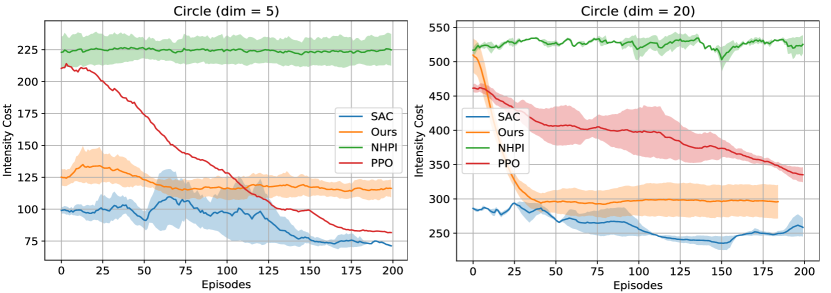
Figure 3: Cumulative intensity cost on synthetic datasets.

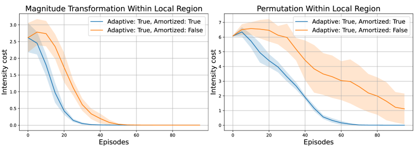
Figure 4: Generalization results of local community transformations on Covid data.

6.2 Evaluating Generalization on Covid Data

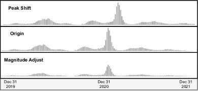
Figure 5: Two types of transformation of Covid data.

Here, our goal is to design an amortized city lock-down strategy that shares a similar policy structure for distinct city regimes to curb the epidemic by intervening in the influence matrix between cities. Concretely, we trained an amortized policy from five different county corpus and tested the amortized interventions on multiple unseen county dynamics. To generalize to an unseen split, the agent needs to be invariant to the orders of different counties and the amplitude or the phase of the spikes of the underlying excitatory point processes. Thus, we evaluated the generalization ability to the unseen counties corpus in two parts, local community transformation, and cross-community adaption, where local community transformation captures the agent’s ability to generalize to a permuted or intensity-adjusted community, and cross-region adaption characterizes the ability to generalize to a intensity-peak-shifted community. We illustrate the two types of transformation in Figure 5.

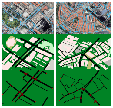
Figure 6: Top: Satellite map extracted from Google Earth (Goo, 2022). Middle: Road Network in SUMO (Lopez et al., 2018). Bottom: Extracted networks where red nodes are junction points.

Generalization Over Local Community Transformation We show the generalization ability to a permutated or intensity-adjusted community by permutating and changing the intensity magnitude on the same community region and applying the amortized policy to them. Figure 4 demonstrates the intensity costs of using amortized policy and not using during learning policies on two types of communities after transformation. For the cost curve on the local community by magnitude transformation, the amortized policy starts to converge at around 30 episodes while the cost of the non-amortized policy is still decreasing. Importantly, we observe the amortized policy also displays a more stable learning curve compared with the non-amortized policy.

Generalization Over Cross Community Adaption We investigate how well the proposed approach generalizes over unseen intensity dynamics from different counties. We evaluate the generalization performance in different county corpus with or without a similar dynamic structure to the training environment. Specifically, we define the testing environment as “in-distribution” or “generalize via interpolation” when the testing environment shares a similar intensity peak to the training environment and define the testing environment as ”out-of-distribution” or “generalize via extrapolation” when the testing environment has a peak-shift or a delay effect to the original training environment. Table 1 summarize the average reduced intensity for different methods under different region settings.

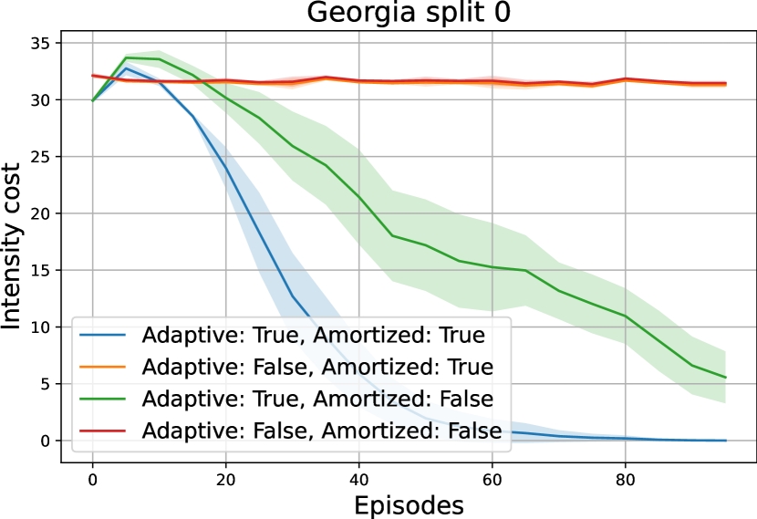
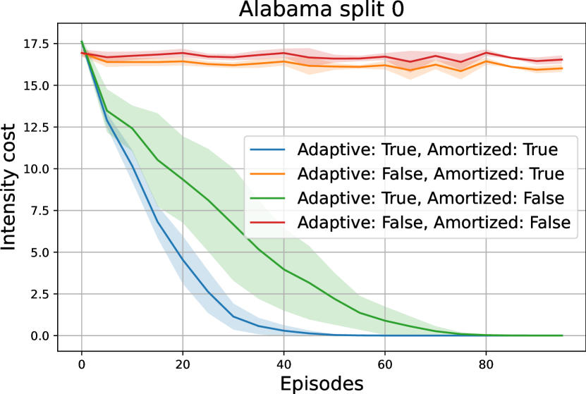
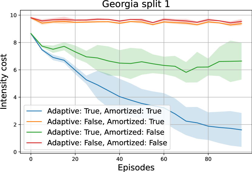
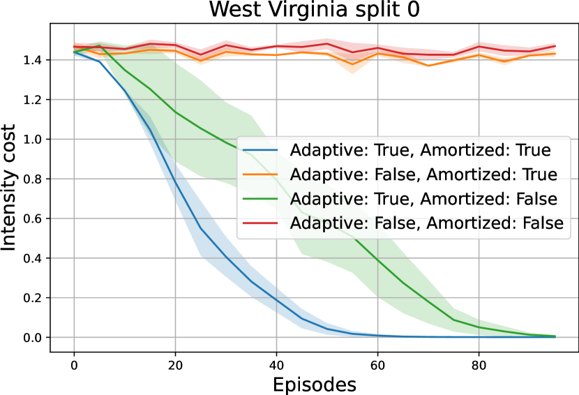
Figure 7: Generalization results for steering covid data on cross-community dynamics.

Notably, Table 1 (1^st row ) indicates that the non-adaptive and non-amortized policies are struggling to control the intensities in both in-distribution and out-of-distribution environments. Importantly, when we use an adaptive but non-amortized policy, the reduced intensities are quite obvious (Table 1, 3^rd row). This is not surprising since adaptively learning a policy (i.e., repeatedly updating the model with new policies) allows the agent to explore more possibilities in the environment and thus can obtain an optimal trajectory more easily. Furthermore, using amortized policy gives a significant jump on both adaptive and non-adaptive policy among all four environments. It is also interesting to point out that in-distribution environments are easier to generalize than out-of-distribution environments which contain a peak-shift or other complex transformations when compared with the trained environment. These findings are also consistent with the intensity cost curves illustrated in Figure 7.

Table 1: Reduced amount of intensities after network interventions for each node per unit time on four unseen communities by different methods. We report average performance across 100 runs for three different seeds, with a standard deviation between parentheses.

Adaptive	Amortized	Reduced Intensities
		In-distribution		Out-of-distribution
		Georgia-0	Alabama-0	Georgia-1	West Virginia-0
False	False	-0.05(0.18)	0.08(0.06)	-0.07(0.11)	-0.02(0.05)
	True	0.21(0.43)	0.18(0.58)	0.06(0.24)	0.02(0.02)
True	False	0.18(0.19)	0.14(0.22)	0.02(0.13)	0.15(0.10)
	True	0.47(0.14)	0.71(0.42)	0.39(0.27)	0.54(0.27)

6.3 Evaluating Generalization on Traffic Data

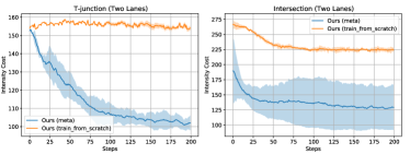
Figure 8: Generalization results of mitigated traffic flow on two unseen intersections from SUMO.

We endeavored to enact network interventions aimed at alleviating traffic congestion within the urban road network system, particularly at road intersections. Event data were collected through SUMO (Lopez et al., 2018) simulations, whereby a traffic car was categorized as contributing to congestion if its velocity dropped below 0.5m/s. The network topology was derived from real-world cartography, as illustrated in Figure 6, and subsequently processed by SUMO to create four distinct crossroad types (detailed information available in Appendix I.1). Following training on these crossroads, we assessed the generalization capabilities of our proposed amortized network intervention method on an additional set of four previously unseen road intersections. As depicted in Figure 8, our results indicate that the learned meta-policy exhibits rapid adaptability to unfamiliar road systems only after a few gradient steps, demonstrating superior traffic congestion mitigation ability compared to a train-from-scratch model. Furthermore, we include a visual representation of the learned network intervention in Appendix I.3.

6.4 Understanding Gains from PEM: Ablations and Visualizations

We show the efficacy of the proposed Policy Equivalent Embeddings (PEE) which are Bi-contrastive metric embeddings (Bi-CMEs) learned with Policy Equivalent Metrics (PEM) on the latent states by comparing it to Policy Similar Embeddings (PSE) (Agarwal et al., 2021) which is another common generalization approach effective on pixel-based RL tasks. Specifically, we investigate the gains from Bi-CMEs and PEM by ablating them. Instead of learning Bi-CMEs jointly through the position and magnitude embeddings, we learn a separate CME for (Chen et al., 2020b) position and magnitude embeddings and use these separately learned embeddings to generate the policies.

Table 2: Ablation studies. Reduced intensity after network interventions on West Virginia (Split 0) when we ablate the similarity metric and learning procedure for metric embeddings in different data augmentation settings. Each ablation entry is repeated for 100 trials for a fair comparison.

Metric / Embedding	CMEs (Perm.)	CMEs (Magn.)	Bi-CMEs
PSM	0.02(0.04)	0.04(0.02)	0.05(0.02)
PEM	0.01(0.06)	0.05(0.02)	0.54(0.27)

Table 2 shows that PEEs (= PEM + Bi-CMEs) generalize significantly better than PSM or Single CMEs, both of which significantly degrade performance (-90%). This is not surprising since policy similar metric (PSM) requires two similar states collected by nearest neighbors which may introduce incorrect clusters on the latent state space. However, by introducing permutation equivalence as an inductive bias to the problem of controlling a dynamic system modeled by neural ODEs, PEM can better characterize the invariance features from different dynamic systems.

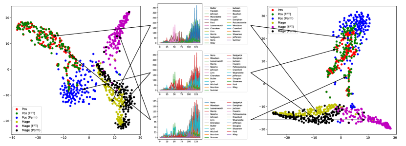
Figure 9: Left: t-SNE of latent embeddings learned with PEM. Middle: Original dynamic of selected 25 counties in Kansas (Top). Perturbed dynamics by two different transformations: random permutation and magnitude adjustment by FFT on the latent space $\mathbf{h}_{t}$ (Middle, Bottom). Right: t-SNE of latent embeddings learned with PSM. PEM successfully disentangle permutation-sensitive position embeddings (blue) and value-sensitive magnitude embeddings (purple).

Visualizing learned representations We visualize the metric embeddings in the ablation above by projecting them to two dimensions with t-SNE. Figure 9 shows that PEEs partition the latent embeddings into four parts: (1) original position embeddings (red) and position embeddings with adjusted magnitude (green); (2) original magnitude embeddings (yellow) and magnitude embeddings with position permuted randomly (blue); (3) position embeddings with position permuted randomly (blue) which are orthogonal to the original position embeddings (red) and (4) magnitude embeddings with adjusted magnitude (purple) which are orthogonal to the original magnitude embeddings (yellow). Nevertheless, the projection of embeddings learned with PSM (Right in Figure 9) gives a clear collapsing effect on position embeddings with position permuted randomly (blue) and magnitude embeddings with adjusted magnitude (purple). This finding is consistent with the results in Table 2 that Bi-CMEs weighted by PSM fail to extract permutation invariant and magnitude invariant information from the latent dynamic system.

7 Conclusions

This paper presents Amortized Networks Intervention, a versatile framework to steer the excitatory point processes. Our approach handles partial observability, fairness constraints, and large-scale network interventions on a combinatorial action space, and achieves promising performance on challenging tasks on large, real-world datasets. Furthermore, the framework discussed here holds the potential for addressing significant problems like traffic light scheduling in urban areas.

Appendix A Related work

As previously highlighted in the introduction, several critical bottlenecks restrict universal applications of prompt control algorithms to disease. When it comes to quickly acquiring new skills, meta-learning emerges as an ideal paradigm for achieving rapid mastery in specific scenarios. In terms of data efficiency, both model-based reinforcement learning (MBRL) and meta-learning have the potential to significantly reduce sample complexity.

Neural Temporal Point Process. In the realm of modeling real-world data, the use of constrained models like Multivariate Hawkes Processes (Hawkes, 1971) can often lead to unsatisfactory results due to model misspecification. In recent studies, researchers have started exploring neural network parameterizations of Temporal Point Processes (TPPs) to mitigate these limitations. Common approaches (Du et al., 2016; Mei & Eisner, 2017) involve the employment of recurrent neural networks to evolve a latent state from which the intensity value can be derived. However, this approach falls short in capturing clustered and bursty event sequences, which are prevalent, as it overlooks vital temporal dependencies or necessitates an excessively high sampling rate (Nickel & Le, 2020).

To surmount these challenges, Neural Jump SDEs (Jia & Benson, 2019) and Neural Spatial Temporal Process (NSTT) (Chen et al., 2020a) extend the Neural Ordinary Differential Equation (ODE) framework, facilitating the computation of exact likelihoods for neural TPPs while addressing the limitations of prior methodologies. These two advancements closely align with our dynamic model, and we draw upon their concepts to develop neural excitatory point processes (EPPs) that are governed by an influence matrix.

Manipulation of Dynamic Processes. The manipulation and control of dynamic processes represent an active area of research. Typically, control policies for temporal process manipulating can be divided into two categories: (1) Gradually introducing exogenous event interventions into the existing historical events, and (2) Promptly enforcing network interventions to the influence matrix between different types of events. Currently, most research is centered around the first type of intervention, primarily focusing on low-frequency and low-dimensional event interventions within social media datasets. For example, techniques like dynamic programming (Farajtabar et al., 2014, 2017) and stochastic control on SDE (Wang et al., 2018) with a closed feedback loop are utilized to steer user activities in social media platforms. However, the number of event types in the above work is limited to derive the closed-form solution. Modern Reinforcement Learning approaches, including both model-free (Upadhyay et al., 2018) and model-based RL (Qu et al., 2023), are proposed to mitigate fake news events on social media. Notably, the event-intervention-based approach will fail to generalize to high frequency and uncontrollable event data like newly infested disease cases and incoming traffic.

On the other hand, the problem of network intervention, particularly node manipulation (e.g., vaccination) to control epidemic processes on graphs has received extensive attention (Hoffmann et al., 2020; Medlock & Galvani, 2009). Most previous studies have adopted a static setup and made a single decision. In recent work (Meirom et al., 2021), the agent performs a sequential decision-making to progressively control graph dynamics through node interventions, demonstrating effectiveness in slowing the spread of infections among different individuals. While existing network-intervention-based approaches offer a promising solution for individual-level quarantine in pandemic control, they do not inherently adapt to county- or state-level control, which necessitates more complex node status considerations than those assumed in (Meirom et al., 2021), as well as a larger search space incorporating edge interventions. Moreover, it’s worth noting that our approach is related to, but more comprehensive than, epidemic control problems, as it accommodates various data distributions, including Poisson, within excitatory point processes.

Model-based Reinforcement Learning. The key to applications within a Reinforcement Learning (RL) framework lies in enhancing sample efficiency, with Model-Based Reinforcement Learning (MBRL) serving the role of approximating a target environment for the agent’s interaction. In environments characterized by unknown dynamics, MBRL can either learn a deterministic mapping or a distribution of state transitions, denoted as $p(\Delta s|[s,a])$. Typically, modeling uncertainty in dynamic systems involves the evolution of a hidden unit to represent a dynamic world model. Several auto-regressive neural network structures are prevalent in this domain, including well-known models such as World Models Ha & Schmidhuber (2018), Decision Transformer (Chen et al., 2021), and the Dreamer family (Hafner et al., 2019, 2023). On the other hand, the integration of Neural Networks with Model Predictive Control (MPC) (Nagabandi et al., 2018) has achieved excellent sample complexity within model-based reinforcement learning algorithms. Our approach closely aligns with MPC and MBRL techniques, wherein MBRL methods, such as Gradient Descent, can be leveraged to refine or adapt the model utilized by MPC. This adaptation holds the potential to enhance performance, especially in scenarios where system dynamics are non-linear, partially unknown, or subject to change.

Meta Reinforcement Learning. The majority of meta Reinforcement Learning (RL) algorithms adhere to a model-free approach and introduce task-specific variational parameters to facilitate learning across various simple locomotion control tasks. Examples of such algorithms include MAESN (Gupta et al., 2018) and PEARL (Rakelly et al., 2019). Simultaneously, there has been notable success in recent times by incorporating the inherent sequential structure of off-policy control into the representation learning process, as demonstrated in works like CURL (Laskin et al., 2020), Sensory (Tang & Ha, 2021), and PSM (Agarwal et al., 2021) particularly when dealing with more complex tasks such as those found in the Distracting DM Control Suite (Stone et al., 2021).

In scenarios where data is limited, such as in disease control, researchers are increasingly focusing on Model-Based Meta Reinforcement Learning (MBMRL), with a specific emphasis on achieving fast adaptation within dynamics models. Approaches like AdMRL (Lin et al., 2020) and Amortized Meta Model-based Policy Search (AMBPS) (Wang & Van Hoof, 2022) involve the optimization and inference of task-specific policies within a parameterized family of tasks, often containing parameters related to positions and velocities. Importantly, a key distinction between our method and AMBPS lies in our utilization of network embeddings and the incorporation of inductive bias to facilitate the learning of a meta-policy without parameterizing individual tasks.

Appendix B Limitations

It should be noted that our approach assumes that decisions made by considering a receding horizon window size of $T$ for each node provide a reasonably good approximation of the optimal policy. However, it is important to acknowledge that if long-range correlations exist, this approximation may result in decreased performance. Consequently, an intriguing question arises regarding the ability of our approach to effectively tackle the problem of network interventions within long-range correlated data distributions under the proposed training protocol.

Appendix C A Comparison Between Neural ODE and Neural Process

In this section, we conduct a comparative analysis of model performance and efficiency between Neural Ordinary Differential Equations (Neural ODE or NODE) (Chen et al., 2018) and Neural Process (NP) (Garnelo et al., 2018). To evaluate these models, we utilized a synthetic dataset consisting of 5-dimensional Multi-Hyperparameter (MHP) data, with each dimension containing 100 sample points in the training set. The results of this comparison are visually presented in Figure 10.

Our observations reveal notable distinctions between the learned behaviors of NODE and the Neural Process model. Specifically, the curve learned by NODE exhibits greater diversity, as depicted in the middle panel of Figure 10. An important metric to consider is the log-likelihood, where we find that Neural ODE achieves a log-likelihood of -33, significantly outperforming Neural Process with a log-likelihood of -180.

It’s essential to consider the computational cost associated with each model. For Neural ODE, a significant portion of the computational burden arises from the numerical integration process itself. The runtime complexity of this integration process is denoted as $O(\text{NFE})$, where NFE represents the number of function evaluations. The worst-case scenario for NFE depends on two factors: the minimum step size $\delta$ required by the ODE solver and the maximum integration time of interest, denoted as $\Delta t_{max}$.

In contrast, the runtime complexity of Neural Process, which employs $n$ context points and $m$ target points, is represented as $O(n+m)$. In our specific experiment, the number of total function evaluations (NFE) for NODE was approximately 5000, while for Neural Process, we selected 50 context points and 100 target points.

It is worth noting that the integration steps, as quantified by $\frac{\Delta t_{max}}{\delta}$, can potentially result in a large constant factor, which may be hidden within the big-O notation. However, it is reassuring to acknowledge that modern ODE solvers, such as dorpi5, are designed with adaptive step size mechanisms that adjust dynamically to the supplied data. This adaptive behavior mitigates concerns related to the scalability of the integration process with respect to dataset size and complexity.

Figure 10: Temporal Point Process Model learned by different methods. Left: ground truth intensity function. Middle: Learned intensity function plot by Neural Jump ODE (Log-Likelihood: -33). Right: Learned intensity function plot by Neural Process. (Log-Likelihood: -183)

Appendix D Technical Details of a Probabilistic Networked Model

Table 3: Table of conditional spike count distributions, their parameterizations, and their properties

Distribution	$p(x|\psi,\upsilon)$	$\mathbb{E}(x)$	Var($x$)
Poi($exp(\psi)$)	$\frac{exp(-exp(\psi))(exp(\psi))^{x}}{x!}$	$exp(\psi)$	$exp(\psi)$
Bern($\sigma(\psi)$)	$\sigma(\psi)^{x}\sigma(-\psi)^{1-x}$	$\sigma(\psi)$	$\sigma(\psi)\sigma(-\psi)$
Bin($\upsilon,\sigma(\psi)$)	$\binom{\upsilon}{x}\sigma(\psi)^{x}\sigma(-\psi)^{\upsilon-x}$	$\upsilon\sigma(\psi)$	$\upsilon\sigma(\psi)\sigma(-\psi)$
NB($\upsilon,\sigma(\psi)$)	$\binom{\upsilon+x-1}{x}\sigma(\psi)^{x}\sigma(-\psi)^{\upsilon}$	$\upsilon\cdot exp(\psi)$	$\upsilon exp(\psi)/\sigma(-\psi)$

Appendix E Technical Details of Mean Field Approximation for Reward Model

To sample multi-stage observations $\{\hat{x}_{n}^{t}\}$ from conditional emission probability distributions $\{\phi^{t}\}$, we have

$$\hat{x}^{1}_{n} \sim\phi^{1}$$ (12)

$$\hat{x}^{2}_{n} \sim\phi^{2}|\hat{x}^{1}_{n}$$ (13)

$$\hat{x}^{3}_{n} \sim\phi^{3}|\hat{x}^{1}_{n},\hat{x}^{2}_{n}$$ (14)

$$\cdots$$ (15)

Thus, we construct a reward model based on the Mean Field Approximation (MFA) for $\hat{x}^{t}_{n}$ by averaging over the high dimensional freedoms on the conditional term, i.e.,

$$\hat{x}^{1}_{n,\text{MFA}} \sim\phi^{1}$$ (16)

$$\hat{x}^{2}_{n,\text{MFA}} \sim\phi^{2}|\ \mathbb{E}_{\phi_{1}}[\hat{x}^{1}_{n,\text{MFA}}]$$ (17)

$$\hat{x}^{3}_{n,\text{MFA}} \sim\phi^{3}|\ \mathbb{E}_{\phi_{1}}[\hat{x}^{1}_{n,\text{MFA}}],\ \mathbb{E}_{\phi^{2}|\ \mathbb{E}_{\phi_{1}}[\hat{x}^{1}_{n,\text{MFA}}]}[\hat{x}^{2}_{n,\text{MFA}}]$$ (18)

$$\cdots$$ (19)

The stochasticity is further ruled out in the reward model by taking the expectation of $\hat{x}^{t}_{n,\text{MFA}}$, i.e.,

$$r^{t}_{n,\text{MFA}}:=\mathbb{E}[\hat{x}^{t+1}_{n,\text{MFA}}]=\mathbb{E}[\mathbb{E}[\hat{x}^{t+1}_{n,\text{MFA}}|\mathbf{h}^{t+1}]]=\mathbb{E}[g_{\lambda_{n}}(\mathbf{h}^{t+1})]$$ (20)

where $\mathbf{h}^{t+1}$ is the latent state of the dynamic system and $g_{\lambda_{n}}$ is the intensity function that can generate the mean value of a count distribution. The second equality follows the law of total expectation and the third expectation is on the distribution of the latent state.

Appendix F Architecture and Hyperparamters

For the dynamic model, we parameterized the ODE forward function $f_{h}$ in Equation equation 3 as a Time-dependent multilayer perception (MLP) with dimensions [64-64-64]. We used the softplus activation function. We first attempted to use MLP to parameterize the instantaneous jump function $\phi_{h}$ in Equation equation 4; however, it led to unstable results for long sequences. Thus we switched to the GRU parameterization, which takes an input, the latent state $\mathbf{h}^{t_{i}}$, and outputs a new latent state. Importantly, we found letting $f_{h}$ and $\phi_{h}$ share all the parameters across different node trajectories will also lead to the failure of capturing the mode diversity. We therefore created an independent biased term added between the MLP layers in $f_{h}$ to compensate for diversity loss. Lastly, we use MLP to parameterize the emission function $g_{\lambda}$.

We initialized all Neural ODEs (for the hidden state) with zero drift by initializing the weights and biases of the final layer to zero. All integrals were solved using (Chen et al., 2018) to within a relative and absolute tolerance of 1E-4 or 1E-6, chosen based on preliminary testing for convergence and stability. We also use Seminorms (Kidger et al., 2021) to accelerate neural ODE learning and apply temporal regularization (Ghosh et al., 2020) to mitigate the effect of stiff ODE systems.

For the policy model, we parameterized the policy network by 4 heads, and 128 d-model Transformer layers. For the synthetic dataset, we used a 2-layer transformer for representation learning and another 2-layer transformer for policy generation. For the real-world dataset, we used a 4-layer transformer for representation learning and another 4-layer transformer for policy generation.

For the Policy Equivalent Metric presented in Definition 2, we learned a value function parameterized by a 2-layer transformer by optimizing Least Square Temporal Difference (LSTD).

We trained the dynamic, policy, and PEM-value network by using the ADAM optimizer with a 1E-2 decay rate across 4 RTX3090 GPUs. The initial learning rates for dynamic learning, policy learning, and PEM-value function learning were set to be 1E-3, 1E-4, and 1E-4 respectively.

Appendix G Additional Details of Synthetic Data Experiment

G.1 Dataset Setup

We generated synthetic networked point process data by simulating Multivariate Hawkes processes (MHP), which are doubly stochastic point processes with self-excitations (Hawkes, 1971). Specifically, the underlying ground truth influence matrix $\mathbf{W}$ was generated with $n=10$ nodes and the weights were set as $w_{ij}\sim\mathcal{U}[0,0.5]$. We set the graph sparsity to 0.1, $i.e.,$ each edge is kept with probability 0.1. The generated influence matrix was adjusted appropriately so that its maximum spectral radius is smaller than one, ensuring the stability of the process. We further set the Hawkes kernel to be an exponential basis kernel, where the parameter was set to $\beta=4$, meaning roughly losing 98% of influence after one unit of time. The simulation of MHP was based on a thinning algorithm (Ogata, 1981) on a $T=100$ horizon.

G.2 Additional Results and Figures

We additionally trained the amortized policy on a synthetic star graph and a circular graph with different ground-truth weight matrices and test the performance on a new star or cycle graph with random weights. The results are shown in Figure 11. Surprisingly, we find the amortized policy only slightly outperforms the non-amortized on both environments. We conjecture this is because we are adapting the amortized policy to a small local region (only 10 nodes) in this experiment so that the non-amortized policy already can achieve relatively good results.

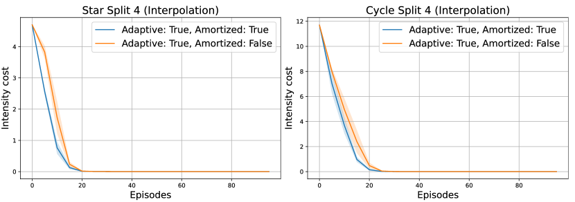
Figure 11: Generalization Results over synthetic data

Appendix H Additional Details of Covid Data Experiment

H.1 Dataset Setup

We used data released publicly by (NYTimes, 2020) on daily COVID-19 to learn the excitatory point processes of the pandemic outbreak. The data contains the cumulative counts of coronavirus cases in the United States, at the state and county level, over time. Specifically, we separated the U.S. COVID-19 data into state-wise records and further split a state-wise record into different county corpus where each split is named as ”a local region” or ”a split”, containing distinct intensity trajectories from no more than 25 counties.

H.2 Additional Results and Figures

We also present the results for different policies under various fairness constraints. Specifically, we use $\lambda_{1}$ to control the weight of an intervention cost and use $\lambda_{2}$ to control the weight of a smoothing cost. The intervention cost used here is defined by the distance between two counties and the smoothing cost is defined by the distance between two consecutive policies between time. We use the average reduced intensity and the average lockdown probability for each edge to measure fairness and the result is shown in Table 4. Interestingly, we find imposing more constraints on the policy ($i.e.,\ \lambda_{1}=0.1,\lambda_{2}=0.1$) does not lead to the lowest lockdown probability. Instead, only enforcing smoothing constraints ($i.e.,\lambda_{1}=0.0,\lambda_{2}=0.1$) gives the fairest policy. We conjecture that adding extra intervention cost constraints will discourage the agent from exploring and thus underperform policy smoothing constraints. We illustrate the detailed lockdown for different constraints in Figure 12.

Table 4: Average lockdown probabilities and reduced intensity under different soft constraints.

Fairness / Parameters	$\lambda_{1}=0.0$		$\lambda_{1}=0.1$
	$\lambda_{2}=0.0$	$\lambda_{2}=0.1$	$\lambda_{2}=0.0$	$\lambda_{2}=0.1$
Average Reduced intensity	0.25(0.06)	0.10(0.04)	0.06(0.05)	0.01(0.03)
Average Lockdown probability (%)	1.31(0.53)	0.43(0.12)	1.29(0.27)	1.29(0.17)

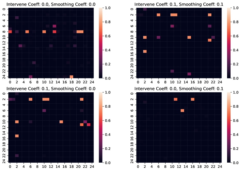
Figure 12: Amortized Networks Interventions in probabilities under different constraints.

Appendix I Additional Details of Traffic Data Experiement

I.1 Dataset Setup

To simulate real-world traffic, based on the road types shown in Figure 6, we design a road network with four types: intersections with one or two lanes, and T-Junction with one or two lanes. Specifically, we let the speed of the road be 8m/s or 11m/s randomly. Then, we generate car trips by the random generation tool from the SUMO package. We make such a simulation for 1000s at one run. After this playing, we can get the simulation results including emissions (e.g. $CO_{2}$, $CO$), positions, speed, and lane id (i.e. the car runs in which lane with lanes more than one in a road) of each car at each time step. Given the generated summary data from SUMO, we then count the congestion event (i.e. the car speed less than 0.5m/s) for the following analysis.

I.2 Additional Results and Figure

We show the intensity cost of the learning process for four types of roads in our simulation setup in Figure 13. For both our model (meta) and our model (train from scratch), the cost trend will converge after several time steps, which proves that our model has great learning and generalization ability.

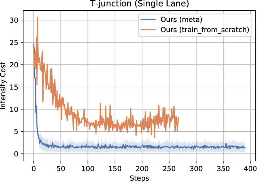
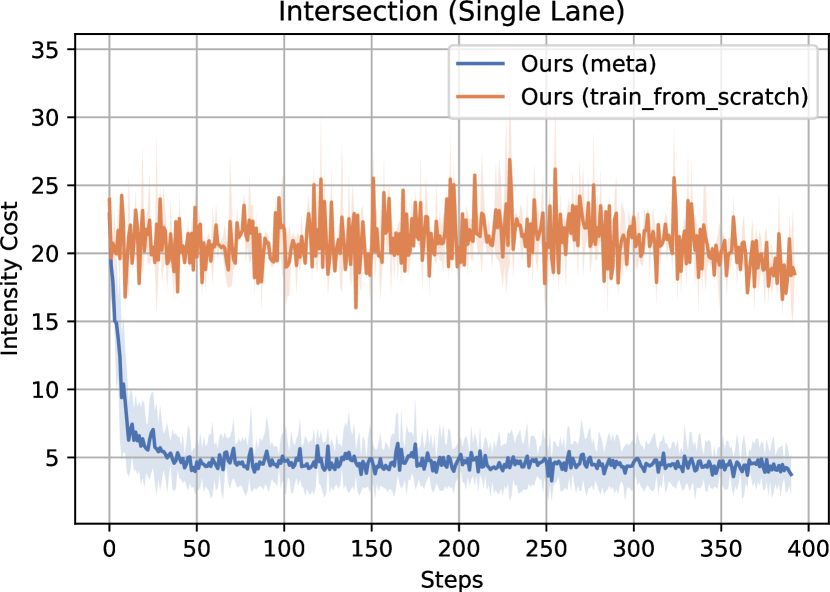
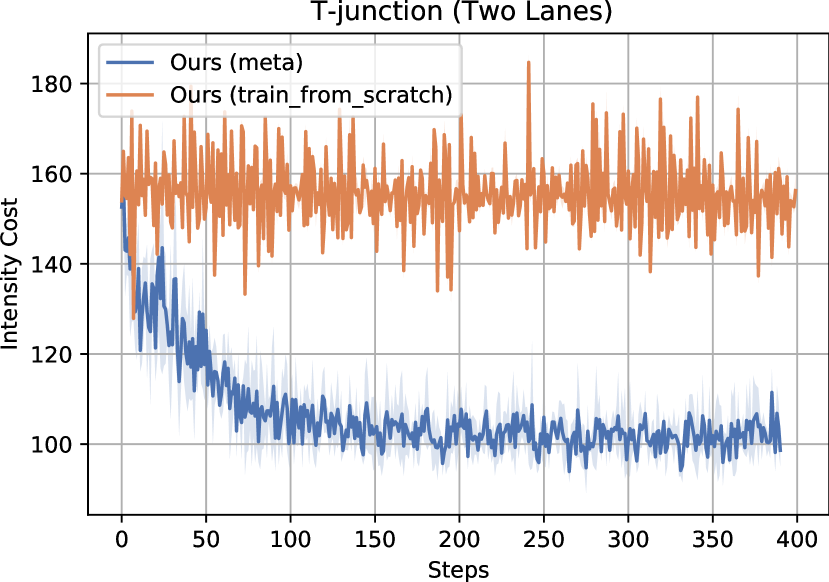
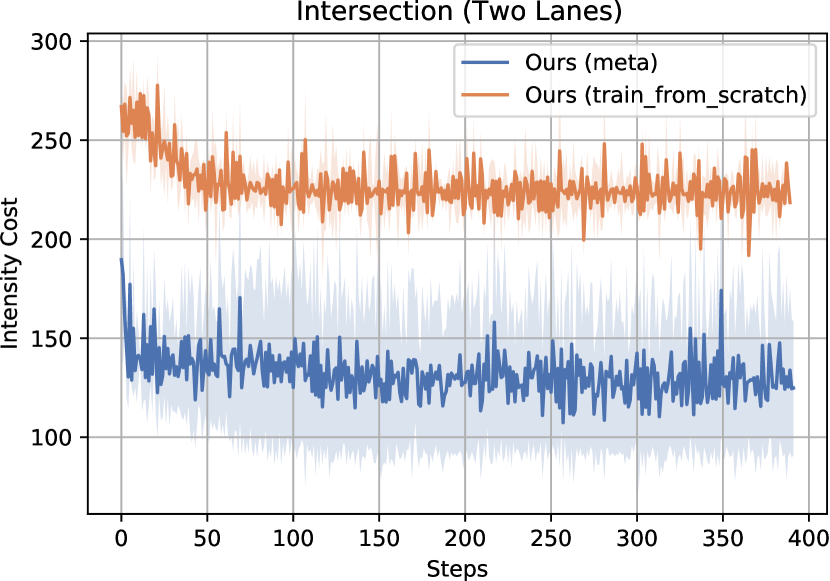
Figure 13: Intensity cost of four types road.

I.3 Case Study

We further provide a case study to show the great interpretation capacity of our model. In the T-junction with single lane scenario, there are 2 discrete actions, corresponding to the following green phase configurations in Figure 14. The traffic light is marked as node 10, while the other three lanes are marked as node 8, node 11, and node 12 in our Sumo simulation setup.

Real-world traffic can be represented as an NJODE model corresponding with the change of traffic lights. In our simulation, when node 10 (i.e. traffic light) becomes green, the lane controlled by this traffic signal will connect, which is represented as 1 in Figure 15; otherwise, the connection between two lanes is disconnected and is represented as 0. For instance, in the first sub-graph of Figure 15, the car can move from node 11 to node 12 under the control of its traffic signal. The learned policy of our model is exactly consistent with real traffic trips, which demonstrates that our model has great adaptation ability in uncovering real-world network interventions.

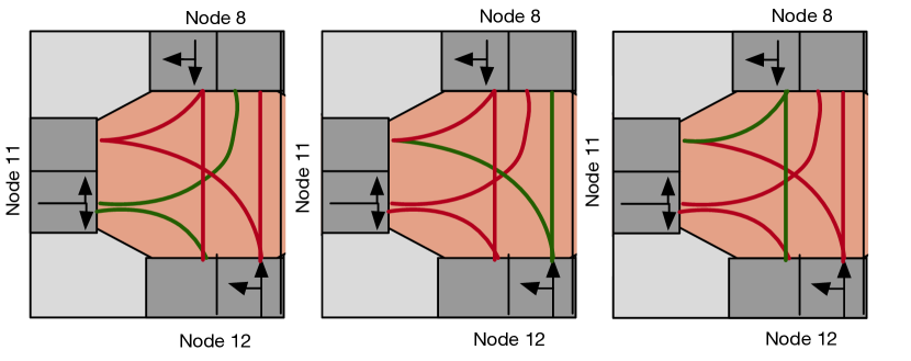
Figure 14: Discrete actions of the T-junction (single lane).

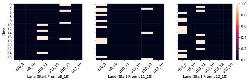
Figure 15: The learned policy of traffic generated from our model.

References

- Goo (2022) Google earth. https://earth.google.com, 2022. Accessed: 10 Sept. 2023.
- Agarwal et al. (2021) Rishabh Agarwal, Marlos C Machado, Pablo Samuel Castro, and Marc G Bellemare. Contrastive behavioral similarity embeddings for generalization in reinforcement learning. International Conference on Learning Representations, 2021.
- Bharadhwaj et al. (2020) Homanga Bharadhwaj, Kevin Xie, and Florian Shkurti. Model-predictive control via cross-entropy and gradient-based optimization. In Learning for Dynamics and Control, pp. 277–286. PMLR, 2020.
- Castro (2020) Pablo Samuel Castro. Scalable methods for computing state similarity in deterministic markov decision processes. In Proceedings of the AAAI Conference on Artificial Intelligence, volume 34, pp. 10069–10076, 2020.
- Chen et al. (2021) Lili Chen, Kevin Lu, Aravind Rajeswaran, Kimin Lee, Aditya Grover, Misha Laskin, Pieter Abbeel, Aravind Srinivas, and Igor Mordatch. Decision transformer: Reinforcement learning via sequence modeling. Advances in neural information processing systems, 34:15084–15097, 2021.
- Chen et al. (2018) Ricky TQ Chen, Yulia Rubanova, Jesse Bettencourt, and David K Duvenaud. Neural ordinary differential equations. Advances in neural information processing systems, 31, 2018.
- Chen et al. (2020a) Ricky TQ Chen, Brandon Amos, and Maximilian Nickel. Neural spatio-temporal point processes. International Conference on Learning Representations, 2020a.
- Chen et al. (2020b) Ting Chen, Simon Kornblith, Mohammad Norouzi, and Geoffrey Hinton. A simple framework for contrastive learning of visual representations. In International conference on machine learning, pp. 1597–1607. PMLR, 2020b.
- Du et al. (2016) Nan Du, Hanjun Dai, Rakshit Trivedi, Utkarsh Upadhyay, Manuel Gomez-Rodriguez, and Le Song. Recurrent marked temporal point processes: Embedding event history to vector. In Proceedings of the 22nd ACM SIGKDD international conference on knowledge discovery and data mining, pp. 1555–1564, 2016.
- Farajtabar et al. (2014) Mehrdad Farajtabar, Nan Du, Manuel Gomez Rodriguez, Isabel Valera, Hongyuan Zha, and Le Song. Shaping social activity by incentivizing users. Advances in neural information processing systems, 27, 2014.
- Farajtabar et al. (2017) Mehrdad Farajtabar, Jiachen Yang, Xiaojing Ye, Huan Xu, Rakshit Trivedi, Elias Khalil, Shuang Li, Le Song, and Hongyuan Zha. Fake news mitigation via point process based intervention. In International conference on machine learning, pp. 1097–1106. PMLR, 2017.
- Garcia et al. (1989) Carlos E Garcia, David M Prett, and Manfred Morari. Model predictive control: Theory and practice—a survey. Automatica, 25(3):335–348, 1989.
- Garnelo et al. (2018) Marta Garnelo, Jonathan Schwarz, Dan Rosenbaum, Fabio Viola, Danilo J Rezende, SM Eslami, and Yee Whye Teh. Neural processes. arXiv preprint arXiv:1807.01622, 2018.
- Ghosh et al. (2020) Arnab Ghosh, Harkirat Behl, Emilien Dupont, Philip Torr, and Vinay Namboodiri. Steer: Simple temporal regularization for neural ode. Advances in Neural Information Processing Systems, 33:14831–14843, 2020.
- Gordon et al. (2019) Jonathan Gordon, John Bronskill, Matthias Bauer, Sebastian Nowozin, and Richard E Turner. Meta-learning probabilistic inference for prediction. International Conference on Learning Representations, 2019.
- Gupta et al. (2018) Abhishek Gupta, Russell Mendonca, YuXuan Liu, Pieter Abbeel, and Sergey Levine. Meta-reinforcement learning of structured exploration strategies. Advances in neural information processing systems, 31, 2018.
- Ha & Schmidhuber (2018) David Ha and Jürgen Schmidhuber. World models. arXiv preprint arXiv:1803.10122, 2018.
- Haarnoja et al. (2018) Tuomas Haarnoja, Aurick Zhou, Kristian Hartikainen, George Tucker, Sehoon Ha, Jie Tan, Vikash Kumar, Henry Zhu, Abhishek Gupta, Pieter Abbeel, et al. Soft actor-critic algorithms and applications. arXiv preprint arXiv:1812.05905, 2018.
- Hafner et al. (2019) Danijar Hafner, Timothy Lillicrap, Jimmy Ba, and Mohammad Norouzi. Dream to control: Learning behaviors by latent imagination. arXiv preprint arXiv:1912.01603, 2019.
- Hafner et al. (2023) Danijar Hafner, Jurgis Pasukonis, Jimmy Ba, and Timothy Lillicrap. Mastering diverse domains through world models. arXiv preprint arXiv:2301.04104, 2023.
- Hawkes (1971) Alan G Hawkes. Spectra of some self-exciting and mutually exciting point processes. Biometrika, 58(1):83–90, 1971.
- Hoffmann et al. (2020) Jessica Hoffmann, Matt Jordan, and Constantine Caramanis. Quarantines as a targeted immunization strategy. arXiv preprint arXiv:2008.08262, 2020.
- Jia & Benson (2019) Junteng Jia and Austin R Benson. Neural jump stochastic differential equations. Advances in Neural Information Processing Systems, 32, 2019.
- Kidger et al. (2021) Patrick Kidger, Ricky TQ Chen, and Terry J Lyons. ” hey, that’s not an ode”: Faster ode adjoints via seminorms. In ICML, pp. 5443–5452, 2021.
- Laskin et al. (2020) Michael Laskin, Aravind Srinivas, and Pieter Abbeel. Curl: Contrastive unsupervised representations for reinforcement learning. In International Conference on Machine Learning, pp. 5639–5650. PMLR, 2020.
- Lighthill & Whitham (1955) Michael James Lighthill and Gerald Beresford Whitham. On kinematic waves ii. a theory of traffic flow on long crowded roads. Proceedings of the royal society of london. series a. mathematical and physical sciences, 229(1178):317–345, 1955.
- Lin et al. (2020) Zichuan Lin, Garrett Thomas, Guangwen Yang, and Tengyu Ma. Model-based adversarial meta-reinforcement learning. Advances in Neural Information Processing Systems, 33:10161–10173, 2020.
- Lopez et al. (2018) Pablo Alvarez Lopez, Michael Behrisch, Laura Bieker-Walz, Jakob Erdmann, Yun-Pang Flötteröd, Robert Hilbrich, Leonhard Lücken, Johannes Rummel, Peter Wagner, and Evamarie Wießner. Microscopic traffic simulation using sumo. In The 21st IEEE International Conference on Intelligent Transportation Systems. IEEE, 2018. URL https://elib.dlr.de/124092/.
- Medlock & Galvani (2009) Jan Medlock and Alison P Galvani. Optimizing influenza vaccine distribution. Science, 325(5948):1705–1708, 2009.
- Mei & Eisner (2017) Hongyuan Mei and Jason M Eisner. The neural hawkes process: A neurally self-modulating multivariate point process. Advances in neural information processing systems, 30, 2017.
- Meirom et al. (2021) Eli Meirom, Haggai Maron, Shie Mannor, and Gal Chechik. Controlling graph dynamics with reinforcement learning and graph neural networks. In International Conference on Machine Learning, pp. 7565–7577. PMLR, 2021.
- Nagabandi et al. (2018) Anusha Nagabandi, Gregory Kahn, Ronald S Fearing, and Sergey Levine. Neural network dynamics for model-based deep reinforcement learning with model-free fine-tuning. In 2018 IEEE international conference on robotics and automation (ICRA), pp. 7559–7566. IEEE, 2018.
- Nickel & Le (2020) Maximilian Nickel and Matthew Le. Learning multivariate hawkes processes at scale. arXiv preprint arXiv:2002.12501, 2020.
- NYTimes (2020) NYTimes. Coronavirus (covid-19) data in the united states, 2020. URL https://github.com/nytimes/covid-19-data.
- Ogata (1981) Yosihiko Ogata. On lewis’ simulation method for point processes. IEEE transactions on information theory, 27(1):23–31, 1981.
- Qu et al. (2023) Chao Qu, Xiaoyu Tan, Siqiao Xue, Xiaoming Shi, James Zhang, and Hongyuan Mei. Bellman meets hawkes: model-based reinforcement learning via temporal point processes. In Proceedings of the AAAI Conference on Artificial Intelligence, volume 37, pp. 9543–9551, 2023.
- Rakelly et al. (2019) Kate Rakelly, Aurick Zhou, Chelsea Finn, Sergey Levine, and Deirdre Quillen. Efficient off-policy meta-reinforcement learning via probabilistic context variables. In International conference on machine learning, pp. 5331–5340. PMLR, 2019.
- Richards (1956) Paul I Richards. Shock waves on the highway. Operations research, 4(1):42–51, 1956.
- Salathé & Jones (2010) Marcel Salathé and James H Jones. Dynamics and control of diseases in networks with community structure. PLoS computational biology, 6(4):e1000736, 2010.
- Sambaturu et al. (2020) Prathyush Sambaturu, Bijaya Adhikari, B Aditya Prakash, Srinivasan Venkatramanan, and Anil Vullikanti. Designing effective and practical interventions to contain epidemics. In Proceedings of the 19th International Conference on Autonomous Agents and MultiAgent Systems, 2020.
- Schulman et al. (2017) John Schulman, Filip Wolski, Prafulla Dhariwal, Alec Radford, and Oleg Klimov. Proximal policy optimization algorithms. arXiv preprint arXiv:1707.06347, 2017.
- Stone et al. (2021) Austin Stone, Oscar Ramirez, Kurt Konolige, and Rico Jonschkowski. The distracting control suite–a challenging benchmark for reinforcement learning from pixels. arXiv preprint arXiv:2101.02722, 2021.
- Tang & Ha (2021) Yujin Tang and David Ha. The sensory neuron as a transformer: Permutation-invariant neural networks for reinforcement learning. Advances in Neural Information Processing Systems, 34:22574–22587, 2021.
- Upadhyay et al. (2018) Utkarsh Upadhyay, Abir De, and Manuel Gomez Rodriguez. Deep reinforcement learning of marked temporal point processes. Advances in Neural Information Processing Systems, 31, 2018.
- Wang & Van Hoof (2022) Qi Wang and Herke Van Hoof. Model-based meta reinforcement learning using graph structured surrogate models and amortized policy search. In International Conference on Machine Learning, pp. 23055–23077. PMLR, 2022.
- Wang et al. (2018) Yichen Wang, Evangelos Theodorou, Apurv Verma, and Le Song. A stochastic differential equation framework for guiding online user activities in closed loop. In International Conference on Artificial Intelligence and Statistics, pp. 1077–1086. PMLR, 2018.
- Weiss (2013) Howard Howie Weiss. The sir model and the foundations of public health. Materials matematics, pp. 0001–17, 2013.
- Xie & Ermon (2019) Sang Michael Xie and Stefano Ermon. Reparameterizable subset sampling via continuous relaxations. In Proceedings of the 28th International Joint Conference on Artificial Intelligence, IJCAI’19, pp. 3919–3925. AAAI Press, 2019. ISBN 9780999241141.