Particle motion in a rotating dust spacetime: the Bonnor solution

Abstract

We investigate the geometrical properties, spectral classification, geodesics, and causal structure of the Bonnor’s spacetime [Journal of Physics A Math. Gen., 10, 1673 (1977)], i.e., a stationary axisymmetric solution with a rotating dust as a source. This spacetime has a directional singularity at the origin of the coordinates (related to the diverging vorticity field of the fluid there), which is surrounded by a toroidal region where closed timelike curves (CTCs) are allowed, leading to chronology violations. We use the effective potential approach to provide a classification of the different kind of orbits on the symmetry plane as well as to study the motion parallel to the symmetry axis. In the former case we find that as a general feature test particles released from a fixed space point and directed towards the singularity are repelled and scattered back as soon as they approach the CTC boundary, without reaching the central singularity.

I Introduction

General relativistic fluid solutions are typically used to build stellar models, whenever the fluid is distributed within a bounded spacetime region. In order to obtain a physical model Einstein’s field equations are then coupled to the thermodynamical equations, which are all solved by imposing several conditions, e.g., symmetries, equation of state, the fall-off behavior of energy density and pressure and their values at the boundary. A further problem in this case is the matching with an asymptotically flat exterior vacuum solution. If the fluid is filling the whole spacetime, instead, the corresponding solution to the gravitational field equations can be used as a cosmological model. There exists very few classes of exact solutions Stephani:2003tm , most of them being associated with perfect fluids. For instance, according to the Friedmann equations underlying the standard cosmological model the matter-dominated and radiation-dominated epochs are driven by dust and radiation fluids, respectively. The simplest solutions for the stellar interiors are instead those which are static and spherically symmetric, which can be always matched across the spherical boundary to an external solution, which consists in a Schwarzschild spacetime.

Unfortunately, most of the known exact solutions are plagued by the presence of singularities as well as unphysical spacetime regions often associated with chronology violations. This is the reason why they have been poorly investigated since their discovery. The most popular is perhaps the Gödel spacetime Godel:1949ga , which is the prototype for rotating cosmological models. The source of the gravitational field is represented by a dust of particles which are at rest with respect to the coordinates, but form a family of twisting world lines preserving the cylindrical symmetry of the spacetime. Gödel solution admits the existence of closed timelike curves (CTCs), allowing for time travel, so that it has been discarded as describing an unphysical universe.

The aim of the present paper is to study the general properties of the Bonnor’s rotating dust cloud spacetime Bonnor:1977 , belonging to the Van Stockum class of stationary and axisymmetric perfect fluid solutions Stephani:2003tm , which are referred to as rigidly rotating dust spacetimes. In fact, the particles of the dust are free falling along the integral curves of the temporal Killing vector. Their angular velocity with respect to locally nonrotating observers equals in magnitude the angular velocity of dragging of inertial frames. The dust particles thus form a geodesic congruence with vanishing expansion ad shear, but nonzero vorticity. Bonnor solution depends on a single parameter, the vanishing of which gives back the flat Minkowskian spacetime. Such a special feature allows for disentangling at any moment genuine curved spacetime properties from special relativistic ones. The arbitrary parameter has the meaning of a rotation parameter, since the metric at spatial infinity reduces to that of a spinning body situated at the origin with angular momentum proportional to it, but with zero mass. Bonnor conjectured the presence of a negative mass distribution contained in the singularity at the center, balancing the positive mass outside, since the density is everywhere positive. The nature of the central singularity in Bonnor spacetime and the possibility to remove it have been further investigated by many authors Bonnor:1980wm ; deAraujo:2000cs ; Bonnor:2005 ; Bratek:2006uw ; Bonnor:2008 ; Gurlebeck:2009vrw . The existence of CTCs has also been extensively studied Bonnor:1980wm ; Steadman:1999 ; Collas:2004hjm ; Collas:2004ydx ; Lindsay:2016xpc . No much attention has been devoted instead to a systematic study of particles motion in Bonnor spacetime. A careful investigation of null geodesic motion can be found in Ref. Steadman:1999 . It has been shown there that there exists a region, or regions, around the origin and the axis of rotation which cannot be entered by null geodesics from spatial infinity. Noticeably, for a wide range of values of the angular momentum photons can be confined in a closed region whose inner boundary is the CTC surface.

In this work we first review the main geometrical properties of the Bonnor spacetime, including the behavior of curvature invariants and the directional character of the central singularity, the spectral classification, and causal structure. We then focus on timelike geodesics, and on how the presence of both the singularity and the CTC surface affects the motion of test particles. The different kind of orbits are classified by using the effective potential approach. In the case of motion on the symmetry plane, some features are familiar from test particle dynamics around compact objects, e.g., circular motion, bound orbits between a minimum and a maximum radius, scattering orbits.

We use a mostly positive signature of the metric and units such that $c=1=G$. Greek indices rum from 0 to 3 while Latin indices from 1 to 3.

II Van Stockum class of perfect fluid solutions

Let us consider a spacetime sourced by a dust fluid, i.e., with energy-momentum tensor $T^{\mu\nu}=\rho_{m}u^{\mu}u^{\nu}$, associated with a metric written in cylindrical-like coordinates $x^{\alpha}\equiv(t,r,\phi,z)$ in the form

$$ds^{2} = ds^{2}_{(t,\phi)}+ds^{2}_{(r,z)}\,,$$ (1)

where

$$ds^{2}_{(t,\phi)} = g_{tt}dt^{2}+2g_{t\phi}dtd\phi+g_{\phi\phi}d\phi^{2}\,,$$

$$ds^{2}_{(r,z)} = g_{rr}dr^{2}+g_{zz}dz^{2}\,,$$ (2)

belonging to the Van Stockum class. All metric and fluid functions depend on $r$ and $z$, and are chosen so that $g_{rr}=g_{zz}=e^{\psi}$, and

$$g_{tt} = -\left(H\gamma^{2}-\frac{r^{2}\chi^{2}}{H\gamma^{2}}\right)\,,$$

$$g_{t\phi} = -\frac{r^{2}\chi}{H\gamma^{2}}\,,$$

$$g_{\phi\phi} = \frac{r^{2}}{H\gamma^{2}}\,,$$ (3)

where we introduced $\gamma=(1-v^{2})^{-1/2}$, as a function of $v$, whose meaning will be clarified below, and $g_{t\phi}/g_{\phi\phi}=-\chi$. The fluid particles move along circular orbits, with four velocity

$$u=\frac{1}{\sqrt{H}}(\partial_{t}+\Omega\partial_{\phi})\,,$$ (4)

where the angular velocity $\Omega$ is given by

$$\Omega=\chi\pm\frac{H\gamma^{2}v}{r}\,,$$ (5)

fixed by the (timelike) normalization condition of $u$, $u~{}\cdot~{}u~{}=-1$. Summarizing: the four functions $H,\chi,\psi,\gamma$ are used to parametrize the metric tensor, and are related by the Einstein’s equations, which are rather involved in this general case, and will not be displayed (see, e.g., Ref. Stephani:2003tm ).

It is also convenient to introduce the lapse-shift notation and write the metric in a form adapted to the Zero-Angular-Momentum-Observers (ZAMOs), with four-velocity

$$n^{\flat}=-Ndt\,,\qquad n^{\sharp}=\frac{1}{N}\left(\partial_{t}-N^{a}\partial_{a}\right)\,,$$ (6)

namely

$$N=\gamma\sqrt{H}\,,\qquad N^{r}=0\,,\qquad N^{\phi}=-\chi\,,\qquad N^{z}=0\,,$$ (7)

so that the metric in ZAMO-adapted form reads

$$ds^{2} = -N^{2}dt^{2}+g_{ab}(dx^{a}-N^{a}dt)(dx^{a}-N^{a}dt)$$ (8)

$$= -H\gamma^{2}dt^{2}+\frac{r^{2}}{H\gamma^{2}}\left(d\phi-\chi dt\right)^{2}$$

$$+ e^{\Psi}\left(dr^{2}+dz^{2}\right),$$

and naturally defines a ZAMO-adapted orthonormal (denoted by a hat) frame of 1-forms

$$\omega^{\hat{0}} = \sqrt{H}\gamma dt\,,$$

$$\omega^{\hat{r}} = e^{\Psi/2}dr\,,$$

$$\omega^{\hat{\phi}} = \frac{r}{\sqrt{H}\gamma}\left(d\phi-\chi dt\right)\,,$$

$$\omega^{\hat{z}} = e^{\Psi/2}dz\,,$$ (9)

with dual frame

$$e_{\hat{0}} = n^{\sharp}\,,\qquad e_{\hat{r}}=e^{-\Psi/2}\partial_{r}\,,$$

$$e_{\hat{\phi}} = \frac{\sqrt{H}\gamma}{r}\partial_{\phi}\,,\qquad e_{\hat{z}}=e^{-\Psi/2}\partial_{z}\,.$$ (10)

The fluid four velocity then reads

$$u=\gamma(n\pm ve_{\hat{\phi}})\,,$$ (11)

so that $v=v(r,z)$ is the spatial three-velocity of the dust as measured by the ZAMOs.

III Bonnor solution

As discussed in Refs Astesiano:2022gph , the case of a rigidly rotating dust is obtained imposing $H=1$. In this subclass of solutions $\Omega$ is constant, and with a proper rotation of the coordinate system can be always put consistently to zero. Without any loss of generality we will assume then $u=\partial_{t}$ for the fluid four-velocity. The request $\Omega=0$ imposes on $v(r,z)$ the constraint

$$v=-\frac{A}{r}\,,$$ (12)

where $A=A(r,z)$ satisfies the equations

$$\frac{(\partial_{z}A)^{2}+(\partial_{r}A)^{2}}{r^{2}e^{\Psi}} = 8\pi G\rho_{m}\,,$$ (13)

$$\partial_{rr}A+\partial_{zz}A-\frac{\partial_{r}A}{r} = 0\,.$$ (14)

The function $\Psi$ satisfies the equations

$$\Psi_{,r} = \frac{A^{2}_{,z}-A^{2}_{,r}}{2r}\,,$$

$$\Psi_{,z} = -\frac{A_{,r}A_{,z}}{r}\,,$$ (15)

which have Eq. (14) as a compatibility condition. Separable solutions to Eq. (14) will be reviewed in Appendix A.

We will consider below a particular example of rotating dust, namely Bonnor’s solution Bonnor:1977 , corresponding to

$$A = \frac{m^{2}r^{2}}{\left(r^{2}+z^{2}\right)^{3/2}}\,,$$

$$\Psi = \frac{m^{4}r^{2}\left(r^{2}-8z^{2}\right)}{8\left(r^{2}+z^{2}\right)^{4}}\,,$$ (16)

The metric is then given by

$$ds^{2} = -dt^{2}-2Adtd\phi+\left(r^{2}-A^{2}\right)d\phi^{2}$$ (17)

$$+ e^{\Psi}\left(dr^{2}+dz^{2}\right)\,,$$

and the dust energy density (see Fig. 1) reads

$$\kappa\rho_{m}=\frac{m^{4}\left(r^{2}+4z^{2}\right)}{\left(r^{2}+z^{2}\right)^{4}}e^{-\Psi}\,,$$ (18)

with $\kappa=8\pi G$, entering the matter energy momentum tensor

$$T^{\mu\nu}=\rho_{m}u^{\mu}u^{\nu}=\rho_{m}\delta^{\mu}_{0}\delta^{\nu}_{0}\,.$$ (19)

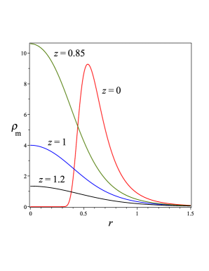
Figure 1: The behavior of the energy density $\rho_{m}(r,z)$ is plotted as a function of $r$ for fixed values of $z=[0,0.85,1,1.2]$, in units of $\kappa$ and assuming $m=1$.

The congruence of world lines tangent to the fluid four velocity $u=\partial_{t}$ is geodesic (vanishing acceleration $a(u)=0$) and shearfree (vanishing expansion $\theta(u)=0$), with nonvanishing vorticity vector (see, e.g., Ref. Jantzen:1992rg for definitions and notations of kinematical quantities)

$$\omega(u)=\frac{e^{-\Psi}m^{2}}{(r^{2}+z^{2})^{5/2}}\left[3rz\partial_{r}-(r^{2}-2z^{2})\partial_{z}\right]\,.$$ (20)

The latter turns out to be aligned with the $z$ axis when evaluated on the symmetry plane ($z=0$),

$$\omega(u)|_{z=0}=-\frac{m^{2}}{r^{3}}\,e^{-\frac{m^{4}}{8r^{4}}}\partial_{z}\,,$$ (21)

and exponentially decaying asymptotically for large $r$. Moreover

$$|\omega(u)|^{2}=\kappa\rho_{m}\,,$$ (22)

as noticed in Ref. Bonnor:1977 .

Unfortunately, Bonnor’s spacetime admits a pathological domain. In fact, the vanishing of the $g_{\phi\phi}$ metric component is responsible for the appearance of an unphysical region characterized by the existence of CTCs

$$r^{2}-A^{2}=0\,,$$ (23)

leading to the following toroidal boundary

$$z_{\rm ctc}=\pm\sqrt{m^{4/3}r^{2/3}-r^{2}}\,.$$ (24)

On the symmetry plane $z_{\rm ctc}=0$, implying that the toroidal region reduces to the circle $r_{\rm ctc}=m$. Even if this can be interesting as a matter of principle, in the following discussion we will not consider physical phenomena in this region.

III.1 Curvature invariants

The Kretschmann invariant for this metric is given by

$$K = R^{\alpha\beta\gamma\delta}R_{\alpha\beta\gamma\delta}$$ (25)

$$= {\mathcal{K}}\frac{m^{4}e^{-2\Psi}}{(r^{2}+z^{2})^{12}}\,,$$

with

$${\mathcal{K}} = -36r^{16}-360r^{14}z^{2}+(8m^{4}-1512z^{4})r^{12}$$ (26)

$$- 3z^{2}(1176z^{4}+m^{4})r^{10}$$

$$+ (-141m^{4}z^{4}-\frac{1}{4}m^{8}-5040z^{8})r^{8}$$

$$- z^{2}(4536z^{8}+293m^{4}z^{4}+3m^{8})r^{6}$$

$$- 3z^{4}(840z^{8}+61m^{4}z^{4}+4m^{8})r^{4}$$

$$- 4z^{6}(198z^{8}-3m^{4}z^{4}+4m^{8})r^{2}$$

$$+ 4z^{12}(-27z^{4}+8m^{4})\,.$$

Taking the limit $r\to\infty$ at fixed $z=$constant yields

$$K=-\frac{36m^{4}}{r^{8}}+\frac{72z^{2}m^{4}}{r^{10}}+O\left(\frac{1}{r^{12}}\right)\,,$$ (27)

whereas for $r\to 0$

$$K = \frac{4m^{4}(8m^{4}-27z^{4})}{z^{12}}$$

$$+ \frac{12m^{4}(4m^{8}-49z^{4}m^{4}+42z^{8})}{z^{18}}r^{2}+O(r^{4})\,.$$

The second quadratic invariant is given by

$${}^{*}K = R_{\alpha\beta\gamma\delta}{}^{*}R^{\alpha\beta\gamma\delta}$$ (29)

$$= {}^{*}{\mathcal{K}}\frac{zm^{6}e^{-2\Psi}}{(r^{2}+z^{2})^{21/2}}\,,$$

with

$${}^{*}{\mathcal{K}} = -18r^{10}-120z^{2}r^{8}-\left(\frac{3}{2}m^{4}+300z^{4}\right)r^{6}$$ (30)

$$- \left(12m^{4}+360z^{4}\right)z^{2}r^{4}$$

$$- (24m^{4}+210z^{4})z^{4}r^{2}-48z^{10}\,.$$

For large values of the radial coordinate at fixed $z$ it behaves as

$${}^{*}K=-\frac{18zm^{6}}{r^{11}}+\frac{69z^{3}m^{6}}{r^{13}}+O\left(\frac{1}{r^{15}}\right)\,,$$ (31)

whereas for $r\to 0$

$${}^{*}K=-\frac{48m^{6}}{z^{10}}-\frac{6m^{6}(-49z^{4}+20m^{4})}{z^{16}}r^{2}+O(r^{4})\,.$$ (32)

Therefore, both invariants diverge approaching $r=0$ for $z\to 0$ only, implying that the singularity at the origin has a directional character, as already discussed by Bonnor himself. In fact, when approaching it along the lines $z=kr$, $r=$constant the argument $\Psi$ of the exponential term changes sign for $1-8k^{2}=0$, so that the curvature invariants as well as the density exhibit different behavior for $\sqrt{r^{2}+z^{2}}\to 0$. No other singularities are present, so that the Bonnor spacetime represents a rotating dust cloud containing an isolated singularity. The latter is not generated by a matter distribution at the center, but rather by the vorticity of the fluid which generally has a divergent behavior there. For instance, for $r\to 0$ at fixed $z$

$$|\omega(u)|^{2}=\kappa\rho_{m}=\frac{4m^{4}}{z^{6}}+\frac{m^{4}(-15z^{4}+4m^{4})}{z^{12}}r^{2}+O(r^{4})\,,$$ (33)

which diverges for $z\to 0$.

III.2 Spectral Petrov type properties

Using $e_{\hat{0}}=n^{\sharp}$ with the corresponding natural adapted spatial frame one can form the null Newman-Penrose tetrad

$$l = \frac{1}{\sqrt{2}}(e_{\hat{0}}+e_{\hat{\phi}})\,,\qquad n=\frac{1}{\sqrt{2}}(e_{\hat{0}}-e_{\hat{\phi}})\,,$$

$$m = \frac{1}{\sqrt{2}}(e_{\hat{r}}+ie_{\hat{z}})\,.$$ (34)

The associated Weyl scalars are $\psi_{1}=0=\psi_{3}$, and

$$m^{2}e^{\Psi}\psi_{0} = \frac{\sum_{k=0}^{3}A_{2k}(\alpha)R^{2k}}{256(\cos(\alpha)m^{2}-R^{2})R^{8}}\,,$$

$$m^{2}e^{\Psi}\psi_{4} = \frac{\sum_{k=0}^{3}B_{2k}(\alpha)R^{2k}}{256(\cos(\alpha)m^{2}+R^{2})R^{8}}\,,$$

$$m^{2}e^{\Psi}\psi_{2} = \frac{m^{4}}{4R^{4}}\left(-3i\sin(\alpha)+\frac{m^{2}(-3\cos(2\alpha)+5)}{12R^{2}}\right)\,,$$

where we have introduced polar coordinates in the $(r,z)$ section of the coordinates

$$r=R\cos\alpha\,,\qquad z=R\sin\alpha\,,$$ (36)

for convenience. The various coefficients are given by

$$A_{0} = (27e^{8i\alpha}+27e^{6i\alpha}-18e^{4i\alpha}-10e^{2i\alpha}$$

$$+7-e^{-2i\alpha})m^{10}\,,$$

$$A_{2} = (54e^{7i\alpha}-36e^{5i\alpha}-48e^{3i\alpha}+36e^{i\alpha}-6e^{-i\alpha})m^{8}\,,$$

$$A_{4} = (-312e^{4i\alpha}-144e^{2i\alpha}+40)m^{6}\,,$$

$$A_{6} = (-480e^{3i\alpha}+96e^{i\alpha})m^{4}\,,$$ (37)

whereas the $B_{i}$ functions are simply related to the $A_{i}$, namely $B_{0}=-A_{0}(-\alpha)$, $B_{2}=A_{2}(-\alpha)$, $B_{4}=-A_{4}(-\alpha)$ and $B_{6}=A_{6}(-\alpha)$. The metric is thus of Petrov type I.

III.3 Timelike geodesics

Let us consider the motion of a massive particle with four-velocity $U=U^{\alpha}\partial_{\alpha}$. The conserved quantities $E=-U_{t}$ (energy per unit of particle mass) and $L=U_{\phi}$ (angular momentum per unit of particle mass) are related to the contravariant components of the four velocity as

$$E=U^{t}+AU^{\phi}\,,\qquad L=AU^{t}+(r^{2}-A^{2})U^{\phi}\,,$$ (38)

so that

$$U^{t}=A\frac{L-EA}{r^{2}}+E\,,\qquad U^{\phi}=\frac{L-EA}{r^{2}}\,,$$ (39)

with $A$ given in Eq. (III). Note that $U^{\phi}$ vanishes when $A=L/E$ (even for $r=$constant motion). The normalization condition $U\cdot U=-1$ implies

$$g_{zz}(U^{z})^{2}+g_{rr}(U^{r})^{2} = \frac{1}{2r^{2}}\left[EA(2L-EA)\right.$$ (40)

$$+ \left.\left(E^{2}-1\right)r^{2}-L^{2}\right]\,.$$

The geodesic equations written in $(t,R,\phi,\alpha)$ coordinates then read

$$\frac{dt}{d\tau} = \frac{-\cos^{2}\alpha m^{4}E-LRm^{2}+R^{4}E}{R^{4}}\,,$$

$$\frac{d\phi}{d\tau} = \frac{\cos^{2}\alpha m^{2}E+RL}{R^{3}\cos^{2}\alpha}\,,$$

$$\frac{d^{2}R}{d\tau^{2}} = \frac{m^{4}\cos^{2}\alpha(9\cos^{2}\alpha-8)}{4R^{5}}\left(\frac{dR}{d\tau}\right)^{2}+\frac{m^{4}\sin\alpha\cos\alpha(-4+9\cos^{2}\alpha)}{2R^{4}}\frac{dR}{d\tau}\frac{d\alpha}{d\tau}$$

$$- \frac{(-8m^{4}\cos^{2}\alpha-4R^{4}+9m^{4}\cos^{4}\alpha)}{4R^{3}}\left(\frac{d\alpha}{d\tau}\right)^{2}+\frac{(2m^{4}E^{2}\cos^{4}\alpha+R^{2}L^{2}+3RELm^{2}\cos^{2}\alpha)}{R^{5}\cos^{2}\alpha}e^{\frac{-m^{4}\cos^{2}\alpha(9\cos^{2}\alpha-8)}{8R^{4}}}\,,$$

$$\frac{d^{2}\alpha}{d\tau^{2}} = -\frac{m^{4}\sin\alpha\cos\alpha(-4+9\cos^{2}\alpha)}{4R^{6}}\left(\frac{dR}{d\tau}\right)^{2}-\frac{(8m^{4}\cos^{2}\alpha-9m^{4}\cos^{4}\alpha+4R^{4})}{2R^{5}}\frac{dR}{d\tau}\frac{d\alpha}{d\tau}$$ (41)

$$+ \frac{m^{4}\sin\alpha\cos\alpha(-4+9\cos^{2}\alpha)}{4R^{4}}\left(\frac{d\alpha}{d\tau}\right)^{2}+\frac{\sin\alpha(-R^{2}L^{2}+m^{4}E^{2}\cos^{4}\alpha)}{\cos^{3}\alpha R^{6}}e^{\frac{-m^{4}\cos^{2}\alpha(9\cos^{2}\alpha-8)}{8R^{4}}}\,,$$

and can be integrated numerically. As an example, we have shown in Fig. 2 the behavior of the integrated orbit in the $r$-$z$ section. The figure also displays the location of the unphysical region containing CTCs. It is interesting to note how the orbit is somehow “repelled” by this region as a typical feature.

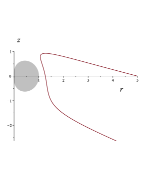
Figure 2: Example of numerical integration of the orbit, Eq. (III.3), projected on the $r$-$z$ plane for the following choice of parameters: $m=1$, $E=1.5$, and $L=-1.8$. Initial conditions are chosen so that $R(0)=5$, $\alpha(0)=0$, $\phi(0)=0$, $t(0)=0$, $\frac{d\alpha}{d\tau}\big{|}_{\tau=0}=0.055$ and $\frac{dR}{d\tau}\big{|}_{\tau=0}\approx-1.0412$, the latter coming from the normalization condition for timelike orbits. The shaded region (grey online) denotes the unphysical region with boundary (24) where CTCs exist.

III.3.1 Motion on the symmetry plane

To study the motion on the symmetry plane ($z=0$, $r_{\rm ctc}=m$) it is convenient to introduce the associated effective potential for radial motion

$$g_{rr}(U^{r})^{2}=\frac{g_{\phi\phi}}{r^{2}}(E-V_{\rm eff}^{r\,+})(E-V_{\rm eff}^{r\,-})\,,$$ (42)

where

$$V_{\rm eff}^{r\,\pm}=\frac{rm^{2}L}{r^{4}-m^{4}}\pm\frac{r^{2}\sqrt{r^{4}+L^{2}r^{2}-m^{4}}}{r^{4}-m^{4}}\,,$$ (43)

which approaches the limiting value $\pm 1$ for large values of $r$. The typical behavior of the (positive branch of the) effective potential as a function of the radial coordinate $r$ is shown in Fig. 3 for selected values of the particle’s angular momentum parameter. Horizontal lines corresponding to fixed values of the particle’s energy parameter intersect the potential curve at the turning points $r^{*}_{i}$ of the radial motion given by the condition $U^{r}=0$, i.e.,

$$r^{*}_{i}=\pm\frac{L}{2\sqrt{E^{2}-1}}+\frac{1}{2(E^{2}-1)^{1/4}}\sqrt{\frac{L^{2}}{\sqrt{E^{2}-1}}\pm 4mE}\,,$$ (44)

where the $\pm$ signs should be chosen independently of each other, and $E>1$. There are at most four real roots (provided that the argument of the square root in the second term is positive), of which one is necessarily negative. Clearly, the number of turning points (depending on the chosen value for the energy) also determines the particular radial motion, either bound or hyperboliclike. Fig. 4 shows some examples of incoming orbits from a given initial value for the radial distance and the same choice of parameters as in Fig. 3.

$$\begin{array}[]{cc}\includegraphics[scale={.35}]{Veff_rad1.eps}&\hskip 28.45274pt\includegraphics[scale={.35}]{Veff_rad2.eps}\cr(a)&(b)\cr\end{array}$$

Figure 3: Typical behavior of the (positive branch of the) effective potential for radial motion as a function of the radial coordinate for $m=1$ (implying that the CTC boundary is at $r_{\rm ctc}=1$) and different values of the particle’s angular momentum parameter. The horizontal lines correspond to different values of the particle’s energy parameter, and intersect the potential curve at the turning points. Left panel: $L=-0.8$; $E=1.01$ (three distinct roots), $E\approx 1.0124$ (three roots, two of them coinciding), and $E=1.015$ (one root). Right panel: $L=-0.2$; $E=1.01$ (one root).

$$\begin{array}[]{cc}\includegraphics[scale={.3}]{plot_equat1.eps}&\hskip 28.45274pt\includegraphics[scale={.3}]{plot_equat2.eps}\cr(a)&(b)\cr\includegraphics[scale={.3}]{plot_equat3.eps}&\hskip 28.45274pt\includegraphics[scale={.3}]{plot_equat4.eps}\cr(c)&(d)\cr\end{array}$$

Figure 4: Examples of numerical integration of the geodesic orbits in the symmetry plane $z=0$. In all plots we have set the value of the parameter $m=1$, and the initial condition for $t$, $\phi$ and $\alpha$ to the values $t(0)=0$, $\phi(0)=0$, $\alpha(0)=0$. The shaded region (grey online) containing CTCs is always displayed, and never crossed by the orbits. Panel (a): parameter choice: $E=1.01$, $L=-0.8$; initial conditions: $R(0)=1.5$, $\frac{dR}{d\tau}\big{|}_{\tau=0}\approx-0.1125$, $\frac{d\alpha}{d\tau}\big{|}_{\tau=0}=0$; turning points: $r_{1}^{*}\approx 1.0625$, $r_{2}^{*}\approx 1.9069$. Panel (b): parameter choice: $E=1.0125$, $L=-0.8$; initial conditions: $R(0)=5$, $\frac{dR}{d\tau}\big{|}_{\tau=0}\approx-0.1043$, $\frac{d\alpha}{d\tau}\big{|}_{\tau=0}=0$; turning points: $r^{*}\approx 1.0479$ (other roots corresponding to imaginary values). Panel (c): parameter choice: $E=1.0124$, $L=-0.8$; initial conditions: $R(0)=5$, $\frac{dR}{d\tau}\big{|}_{\tau=0}\approx-0.1033$, $\frac{d\alpha}{d\tau}\big{|}_{\tau=0}=0$; turning points: $r^{*}\approx 2.5865$ (the one corresponding to the largest values of $r$). Panel (d): parameter choice: $E=1.01$, $L=-0.2$; initial conditions: $R(0)=5$, $\frac{dR}{d\tau}\big{|}_{\tau=0}\approx-0.1418$, $\frac{d\alpha}{d\tau}\big{|}_{\tau=0}=0$; turning points: $r^{*}\approx 2.0554$ (other roots corresponding to imaginary values).

Bound motion is conveniently studied by using an eccentricity-semi-latus rectum parametrization, which is familiar from the Newtonian description of the binary dynamics

$$r=\frac{p}{1+\epsilon\cos\chi}\,,$$ (45)

where $p>m$ and $0\leq\epsilon<1$ are the semilatus rectum and eccentricity, respectively, and $\chi$ the polar angle in the plane of the orbit. The motion is confined between a minimum value $r_{\rm peri}=p/(1+\epsilon)$ for $\chi=0$ and a maximum value $r_{\rm apo}=p/(1-\epsilon)$ for $\chi=\pi$ of the radial coordinate. From Eq. (44) one can then express the particle energy and angular momentum parameters in terms of $(p,\epsilon)$ as follows

$$E = \frac{p^{2}}{\sqrt{p^{4}-m^{4}\epsilon^{2}(1-\epsilon^{2})^{2}}}\,,$$

$$L = -\frac{m^{2}(1+\epsilon^{2})}{p}E\,.$$ (46)

The equation for the radial variable $r$ is thus replaced by the following equation for the angular variable $\chi$

$$\frac{d\chi}{d\tau} = \frac{m^{4}E^{2}}{p^{5}}e^{-\frac{m^{4}(1+\epsilon\cos\chi)^{4}}{8p^{4}}}\epsilon\sin\chi(1+\epsilon\cos\chi)^{2}$$ (47)

$$\times\left[\left(1-\epsilon^{2}+\epsilon\cos\chi\right)^{2}-\epsilon^{2}\right]\,,$$

which can be used to express $t$ and $\phi$ as functions of $\chi$. One can then compute the period $T_{r}$ of the radial motion and the corresponding full variation $\Phi$ of the azimuthal angle

$$T_{r} = \oint dt=2\int_{0}^{\pi}\frac{dt}{d\chi}d\chi\,,$$

$$\Phi = \oint d\phi=2\int_{0}^{\pi}\frac{d\phi}{d\chi}d\chi\,.$$ (48)

The associated radial and azimuthal frequencies are given by $\Omega_{r}=2\pi/T_{r}$ and $\Omega_{\phi}=\Phi/T_{r}$, respectively. Analytical expressions for the above quantities can be obtained in the limit of small eccentricity ($\epsilon\ll 1$) only as power series expansions. The leading order terms turn out to be

$$\Omega_{r} = e^{-\frac{m^{4}}{8p^{4}}}\frac{m^{4}}{2p^{5}\ln(2)}\pi\epsilon+O(\epsilon^{3})\,,$$

$$\Omega_{\phi} = \frac{m^{2}}{p^{3}\ln(2)}\left[2-3\ln(2)-(1-\ln(2))\frac{m^{4}}{2p^{4}}\right]\epsilon^{2}$$ (49)

$$+O(\epsilon^{4})\,.$$

The bound orbit of Fig. 4 (a) corresponds to the parameter choice $p\approx 1.3646$ and $\epsilon\approx 0.2844$. The particle bounces many times between the pericenter and the apocenter before completing a full revolution around the origin. It is interesting to note that the orbit does not reduce to a circular orbit in the limit $\epsilon\to 0$. In fact, in that limit $r$ goes to a constant value, with $E\to 1$ and $L\to-{m^{2}}/{p}$, whereas the frequencies $\Omega_{r}$ and $\Omega_{\phi}$ both vanish, implying that eventually the particle comes to rest.

Finally, circular orbits are obtained by imposing the condition $\partial_{r}V_{\rm eff}^{r\,\pm}=0$, leading to analytical expression for the corresponding radii

$$r_{1\,\rm circ}=-\frac{m^{2}}{L}\,,\qquad r_{2\,\rm circ}=-\frac{m}{L}\sqrt{2m^{2}+\sqrt{L^{4}+4m^{4}}}\,,$$ (50)

for stable ($r_{1\,\rm circ}$) and unstable ($r_{2\,\rm circ}$) orbits, respectively, with $L$ necessarily negative (see also Fig. 3). The solution $r_{1\,\rm circ}$ has associated energy $E=1$ and vanishing $U^{\phi}$ component, so that it actually describes the dust particles which are at rest, as discussed above. The solution $r_{2\,\rm circ}$ instead represents a true circular geodesic with four-velocity

$$U_{\rm circ}=\frac{r^{4}+m^{4}}{r^{2}\sqrt{r^{4}-m^{4}}}\left[\partial_{t}-\frac{m^{2}r}{r^{4}+m^{4}}\partial_{\phi}\right]\,.$$ (51)

The associated energy and angular momentum are given by

$$E_{\rm circ}=\frac{r^{2}}{\sqrt{r^{4}-m^{4}}}\,,\qquad L_{\rm circ}=-\frac{2m^{2}}{r}E_{\rm circ}\,.$$ (52)

The angular velocity $\frac{d\phi}{dt}=-\frac{m^{2}r}{r^{4}+m^{4}}$ tends to the constant value $-\frac{1}{2m}$ as the CTC boundary $r_{\rm ctc}=m$ is approached. $U_{\rm circ}$ then becomes a null vector there (like $\partial_{\phi}$ on the same surface does).

III.3.2 Motion parallel to the symmetry axis

Let us consider the motion parallel to the symmetry axis, i.e., with $r=$ const. One can introduce an effective potential also in this case, such that

$$g_{zz}(U^{z})^{2}=\frac{g_{\phi\phi}}{r^{2}}(E-V_{\rm eff}^{z\,+})(E-V_{\rm eff}^{z\,-})\,,$$ (53)

with

$$g_{zz}V_{\rm eff}^{z\,\pm}=-g_{tz}L\pm r\sqrt{L^{2}+g_{zz}}\,.$$ (54)

In the limit $z\to\pm\infty$ the positive branch of the potential goes to the value $\sqrt{r^{2}+L^{2}}/r$. Turning points for $z$-motion are the real roots of the equation $U^{z}=0$, which can be solved as

$$(r^{2}+z^{2})^{3/2}=-\frac{m^{2}r^{2}E}{L\pm r\sqrt{E^{2}-1}}\,.$$ (55)

For instance, for $L=0$ there are two turning points at $z_{\pm}^{*}=\pm\left[\left(\frac{m^{2}rE}{\sqrt{E^{2}-1}}\right)^{2/3}-r^{2}\right]^{1/2}$. The behavior of the (positive branch of the) effective potential is shown in Fig. 5 for different values of the particle’s angular momentum parameter. Incoming particles endowed with enough energy generally cross the symmetry plane. Low energy particles instead only approach the symmetry plane, and are forced to come back (see Fig. 5 (a)). There also exist conditions allowing for confined motion around $z=0$ or even two opposite values of $z\not=0$, if the particle starts moving close to the symmetry plane with negative values of the angular momentum parameter (see Fig. 5 (a) and (b), respectively).

$$\begin{array}[]{cc}\includegraphics[scale={.35}]{Veff_z1.eps}&\hskip 28.45274pt\includegraphics[scale={.35}]{Veff_z2.eps}\cr(a)&(b)\cr\end{array}$$

Figure 5: Typical behavior of the (positive branch of the) effective potential for motion parallel to the symmetry axis as a function of $z$ for $m=1$, $r=2$ (implying that the orbit does not cross the CTC boundary) and different values of the particle’s angular momentum parameter $L=[-0.8,0,0.8]$ (panel (a)), and $L=-0.2$ (panel (b)).

Circular geodesics on a $z=$ const. ($z\not=0$) hyperplane exist only for $z_{\pm}^{\rm circ}=\pm r/\sqrt{2}$. However, the latter condition implies the vanishing of the angular velocity (with energy parameter $E=1$ and angular momentum parameter $L=-\frac{2\sqrt{6}m^{2}}{9r}$), so that particles actually are at rest there. This is in agreement with the condition $\partial_{z}V_{\rm eff}^{z\,\pm}=0$, which gives

$$z_{\pm}^{\rm circ}=\pm\left[\frac{(mrL)^{4/3}}{L^{2}}-r^{2}\right]^{1/2}\,,$$ (56)

with $0<|L|\leq m^{2}/r$ ($L<0$, see Fig. 5), once $L$ is replaced by the value specified above.

IV Concluding remarks

For a fluid-sourced spacetime the possibility to study gravitational effects as well as particle-particle interactions should be put beside by gravitationally induced collective motion of the fluid particles. This is the case of accreting matter and radiation in the spacetime region around compact objects, for example. In a realistic scenario the thermodynamic properties of the fluid are expected to strongly influence the motion of particles inside it.

The simplest approximation consists in considering a test fluid superposed to the (fixed) gravitational field of the compact object, e.g., a distribution of collisionless dust surrounding a Schwarzschild black hole Bini:2016tqz . The interaction between test particles moving in the background spacetime and the surrounding dust has been modeled there by adding to the equations of motion a friction force built with the stress-energy tensor of the dust, which is responsible for a loss of both energy and angular momentum, causing the particle trajectory to be deflected with respect to the corresponding geodesic path.

In the case of a spacetime sourced by a fluid, instead, it is the matter-energy content of the fluid itself which causes the curvature of the spacetime. The interaction of test particles with the background fluid in a first approximation (i.e., by neglecting particle’s backreaction on the background geometry) is thus described by (timelike) geodesics. While test particle dynamics around black holes is well studied in the literature, the same is not true in the case of fluid-sourced spacetimes. In fact, the latter are in general plagued by the presence of some pathological behavior, like the unphysical behavior of thermodinamical quantities, and the existence of spacetime regions where causality is violated, besides singularities.

In this paper we have investigated test particle motion in the spacetime of a rotating dust, known as Bonnor’s spacetime. The dust particles form a congruence which is geodesic, has vanishing expansion ad shear, but nonzero vorticity. The spacetime has a singularity at the origin of the coordinates, which is not associated with a mass concentrated at the origin as in the case of the gravitational field of a compact object, but rather it is the result of the nonlinearities of the gravitational field due the kinematical properties of the fluid; in particular, its vorticity field, which diverges there. In addition, close to the singularity there exists a toroidal region where CTCs are allowed, which should be discarded as unphysical. The boundary of such a region reduces to a circle on the symmetry plane. We have numerically integrated the geodesic equations with initial conditions chosen such that particles are released from a fixed space point and directed towards the singularity. We found that as a typical behavior particles move inward, but as soon as they approach the boundary of the CTC region they are scattered back. The study of the effective potential for radial motion on the symmetry plane has shown that for most of the allowed values of particle’s energy and angular momentum there is a barrier preventing particles to reach the CTC boundary (and the singularity). We have also found conditions for circular orbits (which are but all unstable) as well as bound motion between a minimum and a maximum radius, which are familiar in the case of test particle motion around compact objects. Rotating dust spacetimes have indeed received a renewed interest in the last years as alternative to supermassive black holes at the center of galaxies Ilyas:2016nio . In addition, their role was studied in connection with galactic dynamics Cooperstock:2006dt ; Balasin:2006cg ; Cooperstock:2005qw ; Astesiano:2022ozl ; Astesiano:2022ghr ; Ruggiero:2023ker ; Ruggiero:2023geh . The results of our work will be useful for a deeper understanding of such connections.

Appendix A Separable solutions to Eq. (14)

In this Appendix we review the construction of separable solutions to Eq. (14), namely

$$\partial_{zz}A+\partial_{rr}A-\frac{1}{r}\partial_{r}A=0\,,$$ (57)

with

$$A={\mathcal{R}}(r){\mathcal{Z}}(z)\,,$$ (58)

obtained in Refs. Cooperstock:2005qw ; Balasin:2006cg . The above ansatz gives

$${\mathcal{Z}}_{zz}=k{\mathcal{Z}}\,,$$ (59)

with the separation constant $k\in R$. Imposing the reflection symmetry property $A(r,z)=A(r,-z)$ leads to two possibilities, according to positive or negative values of $k$.

1. One assumes a positive value for $k:=u^{2}$ (with $u\in R_{0}^{+}$) and the fall off behavior at infinity can be achieved by employing the non-smooth modes ${\mathcal{Z}}(k,z)=e^{-\sqrt{k}|z|}$, which satisfy Eq. (14) for $|z|>0$ only. Consequently, because of the lack of regularity in the metric at $z=0$, there are sources localized at $z=0$. To find an explicit solution in this case one starts from

   $$\tilde{U}(u,z):=\int^{\infty}_{0}A(r,z)J_{1}(ru)dr,$$ (60)

   where $J_{m}(ru)$ is the Bessel function of the order $m$. Then,

   $$\partial_{zz}\tilde{U} = \int^{\infty}_{0}\partial_{zz}A(r,z)\,J_{2}(ru)dr$$ (61)

   $$= -\int^{\infty}_{0}\left(\partial_{rr}A-\frac{1}{r}\partial_{r}A\right)J_{1}(ru)dr\,.$$

   Integration by part gives

   $$\partial_{zz}\tilde{U}=u\int^{\infty}_{0}\partial_{r}A\,J_{0}(ru)dr\,,$$ (62)

   and after another integration by part we get

   $$\partial_{zz}\tilde{U}=u^{2}\int^{\infty}_{0}A\,J_{1}(ru)dr=u^{2}\tilde{U}\,.$$ (63)

   This implies that the required form is $\tilde{U}(u,z)=\alpha(u)e^{-u|z|}+\beta(u)e^{u|z|}$. The asymptotic condition

   $$\lim_{z\rightarrow\infty}A=0,$$ (64)

   implies $\beta(u)=0$ so that

   $$\tilde{U}(u,z) = \alpha(u)e^{-u|z|}$$ (65)

   $$= \int^{\infty}_{0}A(r,z)J_{1}(ru)dr\,.$$

   To obtain the final expression for the function $A$ now it suffices to invert the above relation by using the Hankel transform. The result is

   $$A(r,z)=\int^{\infty}_{0}ru\alpha(u)e^{-u|z|}J_{1}(ru)du\,,$$ (66)

   due to the arbitrariness of $\alpha(u)$ we can redefine a new function using $\tilde{A}(u):=u\alpha(u)$:

   $$\psi(r,z)=\int^{\infty}_{0}re^{-\lambda|z|}\tilde{A}(\lambda)J_{1}(\lambda r)d\lambda,$$ (67)

2. Another possibility is ${\mathcal{Z}}(k,z)=\cosh{(\sqrt{k}z)}$. The parameter $k$ cannot be positive then, otherwise these modes diverge exponentially for $|z|\to\infty$, which is an unphysical behavior. In this case we assume $k=-\lambda^{2}$ with $\lambda\in R_{0}^{+}$ yielding the modes ${\cal Z}(\lambda,z)=\cos{(\lambda z)}$. The solution can be found with the same procedure as in the first case. The result is given by

   $$A(r,z) = \int\limits_{0}^{\infty}d\lambda\cos{(\lambda z)}(r\lambda)\left[a(\lambda)K_{1}(\lambda r)\right.$$ (68)

   $$+ \left.b(\lambda)I_{1}(\lambda r)\right]\,.$$

   The functions $I_{1}$ and $K_{1}$ are modified Bessel functions of the first and second kind, respectively. Since $I_{1}$ blows up exponentially for large values of $r$ we set $b(\lambda)=0$. The function $K_{1}$ falls off exponentially for large values of $r$ and diverges like $1/r$ near $r=0$. However, this divergence is compensated by a linear prefactor, so the integrand is well defined for any sufficiently regular $a(\lambda)$. We can write the result in a simpler form. We perform first a Fourier transformation,

   $$a(\lambda)=\frac{2}{\pi}\int\limits_{0}^{\infty}dx\,C(x)\cos{(\lambda x)}\,,$$ (69)

   where $a(\lambda)$ is determined in terms of a (Fourier) transformed spectral density $C(x)$. Using the property

   $$\int\limits_{0}^{\infty}dxxK_{1}(x)\cos\left(\frac{c\,x}{r}\right)=\frac{\pi}{2}\frac{r^{3}}{(c^{2}+r^{2})^{3/2}}\,,$$ (70)

   the form of $A$ becomes

   $$A(r,z)=\frac{1}{2}\int\limits_{-\infty}^{\infty}d\zeta C(\zeta)\frac{r^{2}}{[(z+\zeta)^{2}+r^{2}]^{3/2}}\,.$$ (71)

References

• (1) H. Stephani, D. Kramer, M. A. H. MacCallum, C. Hoenselaers and E. Herlt, “Exact solutions of Einstein’s field equations,” Cambridge Univ. Press, 2003
• (2) K. Godel, “An Example of a new type of cosmological solutions of Einstein’s field equations of graviation,” Rev. Mod. Phys. 21, 447-450 (1949)
• (3) W. B. Bonnor, “A rotating dust cloud in general relativity,” Journal of Physics A Mathematical General, 10, no. 10, 1673-1677 (1977)
• (4) W. B. Bonnor, “The Rigidly rotating relativistic dust cylinder,” J. Phys. A: Math. Gen. 13, 2121-2131 (1980)
• (5) J. C. N. de Araujo and A. Wang, “Rigidly rotating dust in general relativity,” Gen. Rel. Grav. 32, 1971-1980 (2000) [arXiv:gr-qc/0004082 [gr-qc]].
• (6) W. B. Bonnor, “A rotating dust cloud in general relativity II,” Gen. Rel. Grav. 37, 2245ñ2250 (2005)
• (7) L. Bratek, J. Jalocha and M. Kutschera, “Van Stockum-Bonnor spacetimes of rigidly rotating dust,” Phys. Rev. D 75, 107502 (2007) [arXiv:astro-ph/0603791 [astro-ph]].
• (8) W. B. Bonnor and B. R. Steadman, “Rotating dust clouds in general relativity,” Gen. Rel. Grav. 40, 191ñ198 (2008)
• (9) N. Gurlebeck, “The interior solution of axially symmetric, stationary and rigidly rotating dust configurations,” Gen. Rel. Grav. 41, 2687-2696 (2009) [arXiv:1105.2316 [gr-qc]].
• (10) B. R. Steadman, “Null geodesics in a rotating dust cloud,” Class. Quantum Grav. 16, 3685ñ3691 (1999)
• (11) P. Collas and D. Klein, “Frame dragging anomalies for rotating bodies,” Gen. Rel. Grav. 36, 1197 (2004) [arXiv:0811.2471 [gr-qc]].
• (12) P. Collas and D. Klein, “Causality violating geodesics in Bonnor’s rotating dust metric,” Gen. Rel. Grav. 36, 2549 (2004) [arXiv:0811.2468 [gr-qc]].
• (13) D. S. Lindsay, “Pathologies of van Stockum dust/Tipler’s time machine,” Gen. Rel. Grav. 48, no.9, 121 (2016)
• (14) D. Astesiano, “Rigid rotation in GR and a generalization of the virial theorem for gravitomagnetism,” Gen. Rel. Grav. 54 (2022) no.7, 63 [arXiv:2201.03959 [gr-qc]].
• (15) R. T. Jantzen, P. Carini and D. Bini, “The Many faces of gravitoelectromagnetism,” Annals Phys. 215, 1-50 (1992) [arXiv:gr-qc/0106043 [gr-qc]].
• (16) D. Bini and A. Geralico, “Schwarzschild black hole embedded in a dust field: scattering of particles and drag force effects,” Class. Quant. Grav. 33, no.12, 125024 (2016) [arXiv:1808.05826 [gr-qc]].
• (17) B. Ilyas, J. Yang, D. Malafarina and C. Bambi, “Observational properties of rigidly rotating dust configurations,” Eur. Phys. J. C 77, no.7, 461 (2017) [arXiv:1611.03972 [gr-qc]].
• (18) F. I. Cooperstock and S. Tieu, “Galactic Dynamics via General Relativity: A Compilation and New Developments,” Int. J. Mod. Phys. A 22, 2293-2325 (2007) [arXiv:astro-ph/0610370 [astro-ph]].
• (19) F. I. Cooperstock and S. Tieu, “General relativity resolves galactic rotation without exotic dark matter,” [arXiv:astro-ph/0507619 [astro-ph]].
• (20) H. Balasin and D. Grumiller, “Non-Newtonian behavior in weak field general relativity for extended rotating sources,” Int. J. Mod. Phys. D 17, 475-488 (2008) [arXiv:astro-ph/0602519 [astro-ph]].
• (21) D. Astesiano and M. L. Ruggiero, “Galactic dark matter effects from purely geometrical aspects of general relativity,” Phys. Rev. D 106, no.4, 044061 (2022) [arXiv:2205.03091 [gr-qc]].
• (22) D. Astesiano and M. L. Ruggiero, “Can general relativity play a role in galactic dynamics?,” Phys. Rev. D 106, no.12, L121501 (2022) [arXiv:2211.11815 [gr-qc]].
• (23) M. L. Ruggiero and D. Astesiano, “A tale of analogies: gravitomagnetic effects, rotating sources, observers and all that,” [arXiv:2304.02167 [gr-qc]].
• (24) M. L. Ruggiero, “Stationary rotating and axially symmetric dust systems as peculiar General Relativistic objects,” [arXiv:2306.04832 [gr-qc]].