From Zero to Hero: Detecting Leaked Data through Synthetic Data Injection and Model Querying

Abstract.

Safeguarding the Intellectual Property (IP) of data has become critically important as machine learning applications continue to proliferate, and their success heavily relies on the quality of training data. While various mechanisms exist to secure data during storage, transmission, and consumption, fewer studies have been developed to detect whether they are already leaked for model training without authorization. This issue is particularly challenging due to the absence of information and control over the training process conducted by potential attackers.

In this paper, we concentrate on the domain of tabular data and introduce a novel methodology, Local Distribution Shifting Synthesis (LDSS), to detect leaked data that are used to train classification models. The core concept behind LDSS involves injecting a small volume of synthetic data–characterized by local shifts in class distribution–into the owner’s dataset. This enables the effective identification of models trained on leaked data through model querying alone, as the synthetic data injection results in a pronounced disparity in the predictions of models trained on leaked and modified datasets. LDSS is model-oblivious and hence compatible with a diverse range of classification models, such as Naive Bayes, Decision Tree, and Random Forest. We have conducted extensive experiments on seven types of classification models across five real-world datasets. The comprehensive results affirm the reliability, robustness, fidelity, security, and efficiency of LDSS.

ACM Reference Format:
ACM Conference, XX(X): XXX-XXX, 20XX.
doi:XX.XX/XXX.XX

1. Introduction

It is of paramount importance to protect data through strict enforcement of authorized access. Leaked data can cause profound consequences, from exposing an individual’s private information to broader implications such as reputational damage. More critically, it might result in the loss of competitive business advantages (Cheng et al., 2017), violations of the data owner’s legal rights such as privacy(Shklovski et al., 2014), and breaches of national security (Bellia, 2011). Considerable efforts have been dedicated to enhancing data security, focusing on ensuring secure storage and transfer and adding watermarks to the data so that leaked data can be identified and the owner’s Intellectual Property (IP) can be safeguarded through legal channels. Such watermarking techniques are typically employed in images and videos by embedding either visible or concealed information in the pixels to denote ownership (Huang et al., 2000; Potdar et al., 2005; Cox et al., 2007; Bi et al., 2007).

With the evolution of machine learning and artificial intelligence techniques, new and nuanced threats surface beyond conventional concerns about data theft and publication. Notably, malicious entities who gain access to leaked datasets often utilize them to train models, seeking a competitive edge. For instance, such training models can be exploited for commercial endeavors or to derive insights from datasets that were supposed to remain inaccessible. This emerging threat remains underexplored, and traditional digital watermarking methods might fall short in ensuring traceability, especially in a black-box setting where one can only access a model through a query interface (Ribeiro et al., 2015).

In this paper, we attempt to address the emerging threat of detecting leaked data used for model training. We introduce a novel method, Local Distribution Shifting Synthesis (LDSS), designed to achieve exemplary detection precision on such leakage. Our study focuses on tabular datasets. For image and video datasets, existing work such as training models on watermarked or blended images (Zhang et al., 2018) and label flipped images(Shafahi et al., 2018; Adi et al., 2018) remain effective. This is because researchers often employ Deep Neural Networks (DNNs) on such datasets, where subtle watermarks can be seamlessly integrated without compromising model efficacy yet still be retained for identification purposes. Nonetheless, a substantial number of sensitive datasets, like those pertaining to patients or financial information, are stored in tabular format within relational databases. They typically possess fewer features compared to images with thousands of pixels. Without meticulous design, embedding a ”watermark” into a limited number of columns could severely compromise model accuracy. Moreover, such alterations might go unnoticed by the machine learning model, especially when simpler models like Decision Tree, Support Vector Machine, and Random Forest are employed for these types of tabular datasets. Specifically, we concentrate on the classification task, as many functions in the financial and healthcare sectors hinge on classification. Examples include determining a patient’s susceptibility to specific diseases based on screening metrics (Palaniappan and Mandic, 2007; Huang et al., 2007) as well as assessing if an applicant qualifies for a loan based on their data (Sheikh et al., 2020; Bhatore et al., 2020). Additionally, we assume that only black-box access to the target model is available. This is because unauthorized parties who engage in data theft typically do not disclose their model details, providing only a query interface instead.

Detecting leaked data utilized for model training solely through model querying is non-trivial. At first glance, employing the membership inference attack (Shokri et al., 2017) appears to be a straightforward yet effective solution. However, unauthorized entities can counteract this by applying model generalization techniques (Truex et al., 2021). They might strategically prompt the model to produce incorrect predictions for queries that precisely match instances in their training data, thereby evading detection. Furthermore, this solution sometimes yields a high false-positive rate. This is especially true if the allegedly leaked data originates from a commonly accessed source. In such cases, the third party might coincidentally possess a similar dataset, which could have closely related or even identical instances.

There exist various watermarking and backdoor mechanisms (Li et al., 2021; Xue et al., 2021; Boenisch, 2021) that are designed to embed information into target models. Subsequently, this information can be extracted with high precision to assert ownership. Nevertheless, most of these methods predominantly target the image classification task using DNN models (Zhang et al., 2020, 2021b; Fei et al., 2022; Peng et al., 2023). This preference arises from the rich parameters inherent in DNN models, which facilitate the embedding of additional information without compromising model performance. Their techniques, however, are not suitable for the problem of leaked data detection we explore in this paper. Tabular data, frequently used in fields like healthcare and finance where explainability is paramount, often employ non-DNN models. Moreover, dataset owners lack access to, control over, or even knowledge about the model training process in leaked data scenarios. Therefore, most extant methods in model watermarking (Darvish Rouhani et al., 2019; Namba and Sakuma, 2019) and data poisoning or model backdoor (Chen et al., 2017; Saha et al., 2020) fall short as they typically target a specific model type and necessitate access or control of the training process to guarantee optimal and effective embedding.

To overcome the above challenges, LDSS adopts a model-oblivious mechanism, ensuring robust leaked data detection across different model types and training procedures. The conceptual foundation of LDSS is inspired by the application of active learning and backdoor attacks used to embed watermarks into DNN models (Adi et al., 2018). Rather than merely employing random label flipping, LDSS adopts a more nuanced strategy named synthetic data injection, i.e., it injects synthetic samples into the empty local spaces unoccupied by the original dataset, thereby altering local class distributions. This technique obviates the need to modify or remove existing data instances, preserving the original distribution within the occupied local spaces. Consequently, the classification model trained with these injected samples remains at a similar level of accuracy, while the synthetic injections produce predictions that are substantially different in the affected local spaces compared to models trained without such injections. This ensures a low rate of false positives, even for models trained on datasets with identical samples or those derived from similar populations.

Once the owner modifies the dataset, any subsequent data acquired by an attacker will be this modified version. The leaked data detection is executed by model querying, i.e., querying the suspect model using a trigger set of synthetic samples that are drawn from the same local space as the previously injected samples. To rigorously assess the performance of LDSS, we employed a comprehensive set of evaluation metrics across seven types of classification models. While these models share common objectives, their underlying principles and distinctive characteristics offer a holistic perspective on LDSS’s performance under diverse conditions. Our extensive experimental results, spanning five real-world datasets, showcase the superior performance of LDSS compared to two established baselines. Importantly, these outcomes underscore its reliability, robustness, fidelity, security, and efficiency.

Organization

The rest of this paper is organized as follows. The problem of leaked data detection is formulated in Section 2. We introduce LDSS in Section 3. Experimental results are presented in Section 4. Section 5 reviews related work. Finally, we conclude this work in Section 6.

2. Problem Formulation

In this section, we begin by formally defining the problem of leaked data detection. Following that, we draw comparisons to the problem of model backdooring through data poisoning. Lastly, we outline the criteria for an ideal solution for leaked data detection. Table 1 summarizes the frequently used notations in this paper.

Table 1. List of frequently used notations.

Symbol	Description
$\mathcal{D}_{orig}$	Owner’s original dataset without modifications
$n$	The number of samples in $\mathcal{D}_{orig}$
$d$	The number of features in $\mathcal{D}_{orig}$
$\mathcal{D}_{inj}$	Synthesized samples to be injected into $\mathcal{D}_{orig}$
$\mathcal{D}_{mod}$	Owner’s modified dataset that replaces $\mathcal{D}_{orig}$ by adding $\mathcal{D}_{inj}$ into $\mathcal{D}_{orig}$
$\mathcal{D}_{trig}$	Synthesized dataset similar to $\mathcal{D}_{inj}$, which is used to query the target model for ownership detection
$k$	An integer value for numerical feature discretization
$m$	The number of pivots for data transformation
$\rho$	The injection ratio, i.e., $\rho=|\mathcal{D}_{inj}|/|\mathcal{D}_{orig}|$
$g$, $h$	The number of empty balls and synthesized samples within each ball, respectively

Definition of Leaked Data Detection

In this work, we investigate the problem of leaked data detection, which includes two parties: dataset owners and attackers. The owner has a tabular dataset denoted by $\mathcal{D}_{orig}$, which is structured as a table comprising $n$ rows and $d$ feature columns, along with an additional column designated for class labels. Consequently, each row in this table represents a distinct sample instance. Attackers are assumed to have circumvented security measures and gained unauthorized access to the owner’s dataset. They then train a classification model using the designated label column and deploy it as a service. This model can be developed through any data processing techniques, training procedures, and various model types. The objective is to develop a reliable method that allows dataset owners to ascertain, in a black-box setting, whether a given model has been trained using their dataset. We also explore possible adaptive attacks, assuming that attackers know the proposed method and possess certain information, such as the class distribution and feature ranges from which $\mathcal{D}_{orig}$ is drawn. However, we assume that they lack more detailed insights, such as the distribution of features by class or local class distribution at any subspace. This problem is challenging as dataset owners lack access to the internal parameters of the target model, and their interaction is restricted to submitting queries and receiving corresponding predicted labels.

Comparisons to Model Backdooring through Data Poisoning

This problem closely resembles the objective of model backdooring through data poisoning (Adi et al., 2018; Zhang et al., 2018). We aim to transform the owner’s original dataset, $\mathcal{D}_{orig}$, into a modified version, $\mathcal{D}_{mod}$, ensuring that a model trained on either dataset will exhibit discernible differences in its predictions. Given that we operate under a black-box verification setting, our means of differentiation is to compare the predicted labels of designated trigger samples. Nevertheless, there are three pivotal differences between our problem and the problem of model backdooring via data poisoning:

1. Our primary goal is to empower dataset owners to verify and claim ownership of their dataset through a model trained on it. Unlike strategies that might degrade model performance or embed malicious backdoors, the proposed method should have a minimal impact on both the dataset and the models trained on the modified version.

2. Distinct from model backdooring, this research investigates a defense scenario where defenders do not require any knowledge or access to the attacker’s target model. Defenders can only interact with the model through model querying once the attacker has completed training. Thus, the proposed solution should not make assumptions or modify the model’s architecture, type, or training procedures.

3. In the context of model backdooring through data poisoning, the poisoned dataset is typically inaccessible to parties other than the attackers, making it extremely difficult to detect or locate the backdoor in the trained model. However, for the problem at hand, we assume that attackers have complete access to the modified dataset. This necessitates that any modifications to the dataset should be as discreet as possible to avoid detection and reversal by adversaries.

The key differences outlined above make it challenging to apply existing solutions of model backdooring through data poisoning directly. This includes random label flipping (Adi et al., 2018; Zhang et al., 2018) and training-time model manipulations like manipulating decision boundaries or parameter distributions (Le Merrer et al., 2020). The former is susceptible to detection as outliers, while the latter assumes complete control of the training procedure.

Criteria for An Ideal Solution

To address the first challenge, the proposed solution should abstain from altering samples in $\mathcal{D}_{orig}$. It must be crafted to minimize the impact on model accuracy for unseen samples drawn from the same population as $\mathcal{D}_{mod}$. To overcome the second and third challenges, the proposed method should be agnostic to the attackers’ model training protocols. Furthermore, the injected samples should be meticulously designed to closely mirror the original dataset, thereby enhancing stealth and reducing the risk of detection. Next, we introduce a novel approach, LDSS, which fulfills these stipulated criteria.

3. LDSS: The Methodology

3.1. Overview

LDSS allows data owners to inject a series of synthetic samples, denoted as $\mathcal{D}_{inj}$, into their original dataset, $\mathcal{D}_{orig}$. This strategy is designed to deliberately shift the local class distribution. Once this injection operation is made, it is assumed that attackers would only have access to the modified dataset, $\mathcal{D}_{mod}$. As a result, for samples similar to the injected ones, any target model trained on $\mathcal{D}_{mod}$ is inclined to yield predictions distinct from the model trained on $\mathcal{D}_{orig}$. Thus, to discern whether the datasets are leaked, data owners can generate a trigger set $\mathcal{D}_{trig}$ from similar distributions as $\mathcal{D}_{inj}$ for model querying.

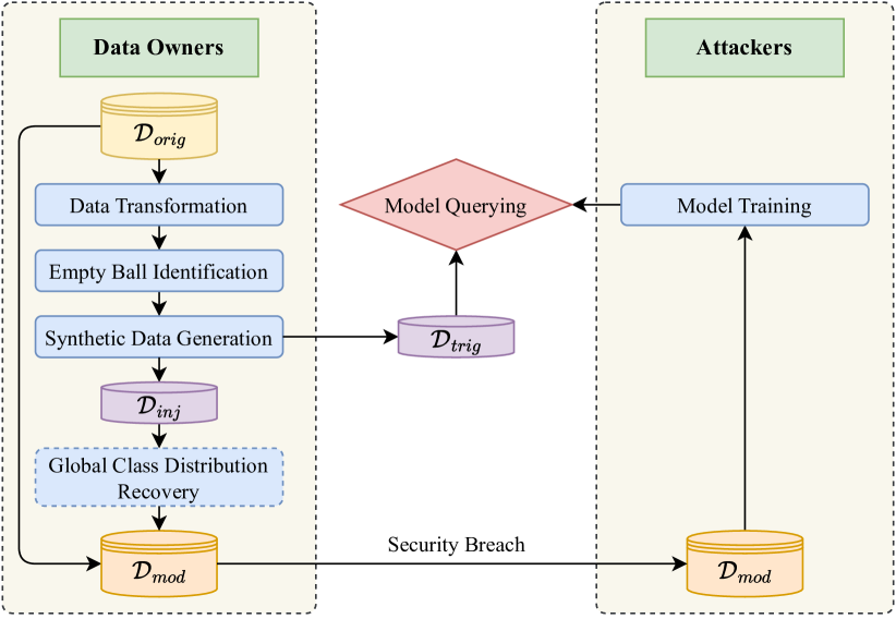
Figure 1. Overall flow of LDSS.

Figure 1 illustrates the overall flow of LDSS. To maintain the model’s efficacy on genuine data resembling the distribution of $\mathcal{D}_{orig}$, LDSS needs to identify large empty balls that are devoid of any samples from $\mathcal{D}_{orig}$ before the synthetic data generation. Nevertheless, the mixed nature of numerical and categorical features in tabular datasets complicates the identification of these large empty spaces. To address this challenge, we initiate a data transformation, converting the tabular dataset to an entirely numerical format. When generating synthetic samples to form an injection set $\mathcal{D}_{inj}$, LDSS synthesize samples within a target class with the most significant frequency disparities relative to the prevailing local class. This strategy can shift the local class distribution. However, it might also drastically alter the global class distribution and become discernible to attackers. To remedy this issue, we could perform an additional step to recover the global class distribution. Details are presented in the following subsections.

3.2. Data Transformation

Challenges. To convert the tabular dataset to a wholly numerical format, a prevalent strategy is to apply one-hot encoding to categorical columns (Chawla et al., 2002). Nevertheless, this strategy can result in extremely high dimensionality, especially when there are a lot of categorical features, each with a multitude of unique values. Not only does computing an empty ball become considerably slower, but such space also becomes very sparse. Thus, the empty ball no longer provides a good locality guarantee. Dimension reduction methods such as Principal Component Analysis (PCA) (Tipping and Bishop, 1999; Minka, 2000; Halko et al., 2011) are unsuitable here since the reduced space should be transformed back to the original space, which contains one-hot encoded features.

To address the aforementioned challenges, we first convert the tabular dataset to an entirely categorical format. This allows us to employ a distance metric, e.g., Jaccard distance, to gauge the proximity between any pair of data. Subsequently, we determine $m$ representative pivots and utilize the Jaccard distance to these $m$ pivots as the numerical representation for each data. The data transformation process encompasses three steps: numerical feature discretization, feature mapping, and numerical representation using pivots. Each of these steps is elucidated as follows.

Step 1: Numerical Feature Discretization

LDSS first discretizes each numerical feature into $(k+1)$ bins using one-dimensional $k$-means clustering. Each bin is assigned a nominal value ranging from $0$ to $k$, in ascending order of their center values. Here, the value of $k$ is chosen to accurately represent the distribution of the feature’s values. To avoid inefficiencies in subsequent steps, $k$ is typically set to a moderate value, such as 5 or 10.

Step 2: Feature Mapping

After the numerical feature discretization, we map each data $\bm{x}=(x_{1},\cdots,x_{d})$ into a set $\bm{\tilde{x}}$ that contains $(k\cdot d)$ elements, with each feature being represented by $k$ elements. This mapping is guided by Equations 1 and 2 as follows:

(1) $$\bm{\tilde{x}}=\textstyle\bigcup_{i=1}^{d}T(i,x_{i}),$$

where

(2) $$T(i,x_{i})=\begin{cases}\{(i,x_{i},j)\mid j\in[1,k]\},&\text{$i$ is categorical};\\ \{(i,x_{i}+j)\mid j\in[1,k]\},&\text{$i$ is numerical}.\end{cases}$$

For each categorical feature, identical values yield the same set of $k$ elements, ensuring that distinct values always produce $k$ distinct elements. For any two numerical values, the number of identical elements among the $k$ elements reflects the closeness of their numerical values. For example, if their categories after discretization are $v_{1}$ and $v_{2}$, then exactly $k-|v_{1}-v_{2}|$ elements will be the same after the feature mapping. The smaller the difference between the original values, the more elements they share after feature mapping. This mapping maintains the degree of similarity between two samples, and such similarity is scaled for numerical features to capture their distributions better.

Step 3: Numerical Representation using Pivots

Finally, we determine $m$ sets as pivots and transform each set $\bm{\tilde{x}}$ into an $m$-dimensional vector $\bm{\hat{x}}=(\hat{x}_{1},\cdots,\hat{x}_{m})\in[0,1]^{m}$, where each coordinate $\hat{x}_{i}$ is represented by the Jaccard distance between $\bm{\tilde{x}}$ and $i$-th pivot. For any two sets $\bm{\tilde{x}}$ and $\bm{\tilde{y}}$, the Jaccard distance is defined as:

(3) $$J(\bm{\tilde{x}},\bm{\tilde{y}})=1-\frac{|\bm{\tilde{x}}\cap\bm{\tilde{y}}|}{|\bm{\tilde{x}}\cup\bm{\tilde{y}}|}.$$

When selecting a small value for $m$, such as 5 or 10, the resulting space has a low dimension, facilitating the efficient identification of empty balls. Moreover, as the Jaccard distance is a distance metric that can effectively gauge the similarity between samples and pivots, samples in close proximity within the transformed space remain similar in the original feature space.

The next challenge is how to determine the pivots to preserve the proximity of the dataset. An initial approach might be to randomly select pivots. In this method, pivots are drawn uniformly at random from $\mathcal{D}_{orig}$. However, this can lead to the selection of suboptimal pivots, especially if certain features in the randomly selected pivots are uncommon. As such, the Jaccard distance between the samples and such pivots can be consistently large. A more refined strategy is to construct pivots based on value frequency. Specifically, for each feature, we identify the top $m$ frequent values. These values are then assigned to the pivots in a round-robin manner. If a feature has fewer than $m$ distinct values, we repeatedly use those values until every pivot has its set of values. This strategy sidesteps the emphasis on infrequent values and also prevents the repetition of unique values, especially when a particular value is overwhelmingly common in specific features. Additionally, this strategy often results in more orthogonal pivots, especially when every feature has at least $m$ unique values. In practice, $m$ can conveniently be set equal to $k$, which is the maximum number of discretized values of each numerical feature so that pivots include all the discretized values of numerical features.

Table 2. Index mapping of transformed elements.

Index	Element
1	(1, F, 1)
2	(1, F, 2)
3	(1, M, 1)
4	(1, M, 2)
5	(2, Cat, 1)
6	(2, Cat, 2)
7	(2, Dog, 1)
8	(2, Dog, 2)
9	(2, Fox, 1)
10	(2, Fox, 2)
11	(3, B, 1)
12	(3, B, 2)
13	(3, W, 1)

Index	Element
14	(3, W, 2)
15	(3, Y, 1)
16	(3, Y, 2)
17	(4, A, 1)
18	(4, A, 2)
19	(4, C, 1)
20	(4, C, 2)
21	(4, G, 1)
22	(4, G, 2)
23	(5, 1)
24	(5, 2)
25	(5, 3)
26	(5, 4)

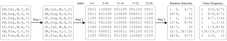
(a) The pipeline of data transformation.

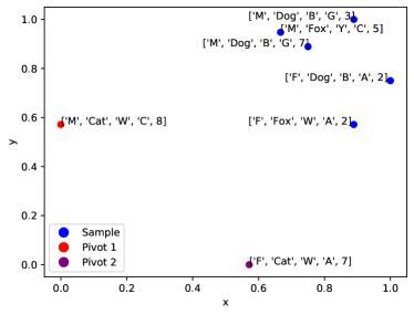
(b) Sample representations by random selection.

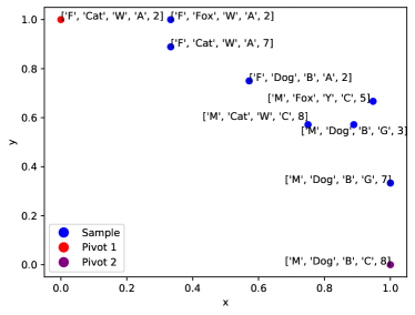
(c) Sample representations by value frequency.

Figure 2. Data transformation results using different pivot selection methods. Note that in Figure 2(b), both pivots come from original samples, while in Figure 2(c), both pivots are constructed based on value frequency. In Figure 2(a), we present the final results using random selection and value frequency, which map to Figures 2(b) and 2(c), respectively.

Example 0:

Suppose a small pet dataset contains 7 samples, as illustrated at the beginning of Figure 2(a). This dataset contains $d=5$ feature columns, namely gender, species, code of color, code of country of origin, and age. The first four features are categorical, while the last one is numerical. Let $m=k=2$.

In step 1, the last numerical feature is discretized into $k+1=3$ bins, with values 2 and 3 in bin 0, 5 in bin 1, and 7 and 8 in bin 2. For example, the first sample becomes $(M,Cat,W,C,2)$. In step 2, each sample is mapped to $kd=10$ elements. Taking the first sample as an example, it maps to the set: $\{(1,M,1)$, $(1,M,2)$, $(2,Cat,1)$, $(2,Cat,2)$, $(3,W,1)$, $(3,W,2)$, $(4,C,1)$, $(4,C,2)$, $(5,3)$, $(5,4)\}$. To streamline our explanation, elements after feature mapping are uniquely indexed, as shown in Table 2. Furthermore, in Figure 2(a), we employ one-hot encoding to transform sets of elements into binary strings. Thus, the first sample is represented as 0011 110000 001100 001100 0011. In step 3, we select two pivots ($k=2$) and compute the Jaccard distance between samples and pivots. For the approach using random selection, e.g., selecting the first and the fifth samples as pivots, the resulting representation is shown in the left column of Figure 2(a) following Step 3. For the approach based on value frequency, e.g., constructing a pair of pivots $(F,Cat,W,A,2)$ and $(M,Dog,B,C,8)$–with the last feature discretized to $0$ and $2$, respectively–the resulting representation is illustrated in the right column of Figure 2(a) after Step 3.

In Figure 2(b) and 2(c), we depict the sample representations of both approaches using scatter plots. These figures highlight that pivots built on value frequency more effectively preserve the relative similarities among samples post-transformation compared to those by random selection. This is because the random pivot selection might incorporate rare or duplicate values for specific features, causing many unique values to become indistinguishable. On the other hand, pivots derived based on value frequency tend to be more orthogonal, thus better maintaining relative similarity. $\triangle$

3.3. Empty Ball Identification

The next step is to identify empty balls in the transformed hypercube $[0,1]^{m}$. Our objective is to locate those empty balls that are both sufficiently large and close to the transformed dataset $\widehat{\mathcal{D}}_{orig}$. Balls located too far from this dataset are considered outliers, making them unsuitable for synthetic data injection. Before delving into our strategy to identify these empty balls, we first define what constitutes an empty ball for numerical features.

Definition of the Empty Ball

Let $\bm{\hat{c}}=(\hat{c}_{1},\cdots,\hat{c}_{m})$ represent the center of an empty ball in the $m$-dimensional transformed space. To define the radius of this empty ball, consider the prevalent Euclidean distance between any two points, $\bm{\hat{x}}=(\hat{x}_{1},\cdots,\hat{x}_{m})$ and $\bm{\hat{y}}=(\hat{y}_{1},\cdots,\hat{y}_{m})$. The distance is given by $\|\bm{\hat{x}}-\bm{\hat{y}}\|=\sqrt{\textstyle\sum_{i=1}^{m}(\hat{x}_{i}-\hat{y}_{i})^{2}}$. With this specific distance, the radius $r$ of the empty ball centered at $\bm{\hat{c}}$ can be defined as:

(4) $$r=\textstyle\min_{\bm{\hat{x}}\in\widehat{\mathcal{D}}_{orig}}\|\bm{\hat{x}}-\bm{\hat{c}}\|.$$

Empty Ball Identification

To prevent the over-clustering of samples generated within the empty balls, which could allow attackers to easily identify injected samples, we prioritize the balls with larger radii over those with smaller ones. Several heuristics, such as the Voronoi diagram and the Evolutionary Algorithm, are available for finding the largest empty ball, as discussed by Lee et al. (2004). However, our goal is merely to identify large empty balls. For enhanced efficiency, we adopt Simulated Annealing (SA) coupled with constrained updates. The procedure is detailed in Algorithm 1.

The algorithm initiates by randomly selecting a batch of $G$ samples (500, in our experiments) from $\widehat{\mathcal{D}}_{orig}$ as seeds (potential centers for empty balls) (Line 1). Then, it continues to replace these seeds with perturbed versions that have a greater radius (Lines 1–1). As iterations progress, the perturbation scale is reduced, governed by the temperature parameter $t$ (Line 1). Given an arbitrary center $\bm{\hat{c}}=(\hat{c}_{1},\cdots,\hat{c}_{d})$, the function $perturb(\bm{\hat{c}},t)$ adds noise that is scaled by $t$ and the standard deviation $std_{i}$ of each dimension $i$ over all samples, i.e., $\hat{c}_{i}^{\prime}=\hat{c}_{i}+t\cdot uniform(-std_{i},std_{i})$. The function $r(\bm{\hat{c}})$ is defined by Equation 4, computing the radius of the empty ball centered at $\bm{\hat{c}}$. In each iteration, ball centers are updated by the perturbed ones that have a larger radius (Line 1). To ensure that the empty balls remain in proximity to $\widehat{\mathcal{D}}_{orig}$ and avoid positioning synthesized samples as potential outliers relative to $\widehat{\mathcal{D}}_{orig}$, only ball centers that are not flagged as outliers by Isolation Forest (Liu et al., 2008), trained on $\widehat{\mathcal{D}}_{orig}$, are considered (Line 1). These selected centers then supersede the prior ones (Line 1). The entire process terminates when $t$ is less than a predefined threshold $\epsilon$ (Line 1).

Given that an adequately large empty ball suffices for generating distant samples, a moderate decrement of $t$ in every iteration, coupled with a small value of $\epsilon$, can ensure good performance without compromising execution speed. In the experiments, we set $\epsilon=0.01$ and decrease $t$ by a factor of 0.8 in each iteration.

Input: Transformed dataset $\widehat{\mathcal{D}}_{orig}\subset[0,1]^{m}$, the number of empty balls $G$, stopping condition $\epsilon$;

Output: A set of empty balls $\mathcal{S}$;

1 $S\leftarrow G$ samples drawn uniformly at random from $\widehat{\mathcal{D}}_{orig}$;

2 $t\leftarrow 1$;

3 while $t\geq\epsilon$ do

4       foreach $\bm{\hat{c}}\in S$ do

5             do

6                   $\bm{\hat{c}}^{\prime}\leftarrow perturb(\bm{\hat{c}},t)$;

7                  

8            while $\bm{\hat{c}}^{\prime}$ is an outlier or $r(\bm{\hat{c}}^{\prime})\leq r(\bm{\hat{c}})$;

9             $\bm{\hat{c}}\leftarrow\bm{\hat{c}}^{\prime}$;

10            

11       $t\leftarrow t\cdot 0.8$;

12      

13return $S$;

Algorithm 1 Empty Ball Identification

3.4. Synthetic Data Injection

Upon identifying $G$ large empty balls, we proceed with two hyperparameters, $g$ ($1\leq g\leq G$) and $h$ for synthetic data injection. This process comprises three steps: empty ball selection, synthetic data generation, and synthetic data injection.

Step 1: Empty Ball Selection

To produce high-quality synthetic data, our goal is to identify empty balls where there is a substantial local frequency gap between the most frequent and least frequent classes. Firstly, we pinpoint the top $g$ empty balls that exhibit the most pronounced local frequency disparities between the highest and lowest frequency classes. Then, leveraging the least frequent class as our target class, we generate $h$ synthetic samples of this class within each of these chosen balls. The local frequency gap is ascertained by counting frequencies within the closest $h$ samples to the ball’s center based on Euclidean distances. This implies that within the local vicinity of $2h$ samples centered around the ball–post the synthetic data injection–the target class will emerge as the dominant one since at least $h$ of the injected samples will bear the same class. Due to the use of SA, Algorithm 1 might produce near-duplicated empty balls. Thus, duplicate removal is performed by shrinking the radius of balls with lower ranks.

Given the ranking criteria for empty balls, we ensure that a minority class takes precedence locally. Thus, this is anticipated to affect the decision-making of a classification model within those localized regions. Note that $g$ is usually small (e.g., 10) to ensure that synthetic samples are concentrated, and $h$ is determined by $g$ and the injection ratio $\rho$, where $\rho$ is defined as the ratio of the number of injected samples, $|\mathcal{D}_{inj}|$, to the number of original samples, $|\mathcal{D}_{orig}|$, i.e., $\rho=|\mathcal{D}_{inj}|/|\mathcal{D}_{orig}|$.

Step 2: Synthetic Data Generation

After identifying the top $g$ empty balls, where each is assigned a designated target class, LDSS synthesizes $h$ samples within each ball to form an injection set. Since our empty balls exist in the transformed space, it is imperative that the resulting samples can be transformed into the original feature space. It is important to emphasize that the direct random generation of samples within each empty ball, followed by their transformation back to the original feature space, is not feasible. The primary reason is the inherent challenge (or the sheer impossibility) of pinpointing a sample that perfectly matches the target Jaccard distances to all the $m$ pivots.

For a dataset with $d$ features, we map each feature into $k$ elements based on Equations 1 and 2. If they share $l$ common elements, their Jaccard distance is given by $J=1-\tfrac{l}{2dk-l}$. Given a Jaccard distance $J$, the number of shared elements can be deduced as Equation 5:

(5) $$l=l(J)=\frac{2dk(1-J)}{2-J}.$$

Considering a distinct value $v^{\prime}$ of feature $i$ in $\mathcal{D}_{orig}$, let $\bm{w}_{v^{\prime}}$ be an $m$-dimensional vector, where its coordinates are the number of shared elements between $v^{\prime}$ and the $i$-th feature of $m$ pivots. Hence, we can calculate the total number of shared elements between the $m$ pivots and a certain sample projected to $\bm{\hat{c}}=(\hat{c}_{1},\cdots,\hat{c}_{m})$ as $\bm{w}_{\bm{\hat{c}}}=(w_{1},\cdots,w_{m})$ such that $w_{j}=l(\hat{c}_{j})$, where $j\in\{1,\cdots,m\}$. Thus, by utilizing the vector $\bm{w}_{v^{\prime}}$ and the target vector $\bm{w}_{\bm{\hat{c}}}$ as a measure of weights, we can reduce this problem to a classical $m$ dimensional knapsack problem (Knuth, 2014).

Consider a bag of infinite capacity and $m$ dimensional weights and a target weight $\bm{w}_{\hat{\bm{c}}}$ to achieve by filling the bag with selected objects. Each available object is identified by a pair ($i,v^{\prime}$) representing feature $i$ of value $v^{\prime}$, and its weight is thus $\bm{w}_{v^{\prime}}$. In this knapsack problem, the weight vector $\bm{w}_{v^{\prime}}$ is non-negative in all $m$ dimensions. There exists one such object for each $i\in\{1,\cdots,d\}$ and possible values $v$ of feature $i$. A total of $d$ objects should be chosen with exactly one for each $i$. The objective is to fill the bag with the chosen $d$ objects such that the total weight $\bm{w}$ is close to $\bm{w}_{\bm{\hat{c}}}$ measured by $L_{\infty}$ distance. Each possible solution consists of exactly $d$ objects representing the values for each feature. Thus, we employ dynamic programming to solve the knapsack problem and synthesize samples as a solution to our original problem. The pseudo-code is presented in Algorithm 2.

Let state $S_{i,\bm{w},v}$ be a Boolean value denoting whether the bag can be filled by $i$ items from the first $i$ features, with $v$ as feature $i$’s value and a total weight $\bm{w}$. Algorithm 2 finds the values of all possible $S_{i,\bm{w},v}$ for all $i\in\{1,\cdots,d\}$ (Lines 2–2). We then chooses among all $S_{d,\bm{w},v}=True$ whose weight vector $\bm{w}$ has the smallest $L_{\infty}$ distance to $\bm{w}_{\bm{\hat{c}}}$ (Line 2). Finally, we backtrack to generate synthetic samples in the original $d$ dimensional space with random values selected for a $v$ if there are different possibilities (Lines 2–2).

It is worth noting that directly executing Algorithm 2 is practically challenging due to the potentially vast number of possible triples $(i,\bm{w},v)$ that $S_{i,\bm{w},v}=True$, especially considering the exponential growth of samples constructed from every possible feature value. We employ an effective approximation by capping the number of possible states for each $i$ at the end of the loop (Lines 2–2). For each $i$, we only keep a limited number of $S_{i,\bm{w},v}=True$ that $\bm{w}$ has smallest $L_{\infty}$ distance to $\bm{w}_{\bm{\hat{c}}}\cdot\tfrac{i}{d}$ by enforcing a similar weight increase rate in all dimensions. In practice, we observe that such a limit between 50,000 and 100,000 is satisfactory. Other optimization includes memorizing only true states and enumerating only at most $(m+1)$ possible feature values instead of all (Line 2).

Input: $\mathcal{D}_{orig}$ and $m$ pivots with $d$ features, an empty ball center $\bm{\hat{c}}\in[0,1]^{m}$ and its target weight vector $\bm{w}_{\bm{\hat{c}}}$, and # generated samples $h$;

Output: Result set $R$;

1 $S_{0,[0]^{m},nil}=True$;

2 for $i=1$ to $d$ do

3       foreach $(\bm{w},v)$ that $S_{i-1,\bm{w},v}=True$ do

4             foreach $v^{\prime}$ in distinct values of feature $i$ in $\mathcal{D}_{orig}$ do

5                   $\bm{w}_{v^{\prime}}\leftarrow$ # shared elements between $v^{\prime}$ and the $i$-th feature of $m$ pivots;

6                   $\bm{w}^{\prime}\leftarrow\bm{w}+\bm{w}_{v^{\prime}}$;

7                   $S_{i,\bm{w}^{\prime},v^{\prime}}=True$;

8                  

9            

10      

11 $T\leftarrow$ $h$ pairs $\{(\bm{w},v)\}$ such that $S_{d,\bm{w},v}=True$ with the smallest $\|\bm{w}-\bm{w}_{\bm{\hat{c}}}\|_{\infty}$;

12 $R\leftarrow\varnothing$;

13 foreach $(\bm{w},v)\in T$ do

14       $\bm{x}=(x_{1},\cdots,x_{d})\leftarrow[0]^{d}$;

15       for $i=d$ to $1$ do

16             $x_{i}\leftarrow v$;

17             $\bm{w}_{v}\leftarrow$ # shared elements between $v$ and the $i$-th feature of $m$ pivots;

18             $\bm{w}^{\prime}\leftarrow\bm{w}-\bm{w}_{v}$;

19             $v^{\prime}\leftarrow$ a random value $v^{\prime}$ that $S_{i-1,\bm{w}^{\prime},v^{\prime}}=True$;

20             $(\bm{w},v)\leftarrow(\bm{w}^{\prime},v^{\prime})$;

21            

22      $R\leftarrow R\cup\{\bm{x}\}$;

23      

24 return $R$;

Algorithm 2 Sample Synthesis within An Empty Ball

Step 3: Synthetic Data Injection

After Algorithm 2 is executed, we find the top $h$ samples with the closest $L_{\infty}$ distance to the ball center. This is repeated for each of the $g$ empty balls to synthesize the total $(g\cdot h)$ samples as injection set $\mathcal{D}_{inj}$. After injecting them into $\mathcal{D}_{orig}$, we get a modified dataset, i.e., $\mathcal{D}_{mod}=\mathcal{D}_{orig}\cup\mathcal{D}_{inj}$.

Assuming that $\widehat{\mathcal{D}}_{orig}$ accurately represents the population, empty balls will either remain unoccupied or be minimally populated in datasets of similar distributions. Thus, this approach guarantees a considerable local distribution shift, even when confronted with a different dataset originating from the same population. It also provides a defense against potential dilution attacks. Should an attacker acquire additional data from the same population and merge it with $\widehat{\mathcal{D}}_{orig}$ for training, the samples injected within these empty balls, which are likely to remain unoccupied in datasets from the same source, will continue to effectively alter the local distribution.

Example 0:

Figure 3 visually conveys the idea of synthetic data injection. The red, green, and light blue points depict the transformed data from 3 different classes in $\widehat{\mathcal{D}}_{orig}$. The grey circle shows an empty ball among them, where the most frequent class is red, and the least frequent class is blue. The model trained on $\widehat{\mathcal{D}}_{orig}$ would likely classify samples within the circle as red. Yet, when injecting 4 dark blue samples labeled similarly to the light blue ones into $\widehat{\mathcal{D}}_{orig}$, the model trained on $\mathcal{D}_{mod}$ would probably predict samples inside the grey circle as blue. This distinction is crucial for determining whether a model was trained using $\mathcal{D}_{mod}$. $\triangle$

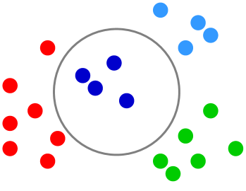
Figure 3. An example illustrates the injection of synthetic samples into an empty ball. By injecting four dark blue points with labels identical to the light blue ones, a model trained on this modified dataset $\mathcal{D}_{mod}$ is more likely to predict samples within the grey circle as blue rather than red.

3.5. Model Querying

To determine whether a target model has been trained on $\mathcal{D}_{mod}$, we can randomly select some samples from $\mathcal{D}_{inj}$ to form a trigger set $\mathcal{D}_{trig}$ and query the target model. However, this way is not optimal, as attackers could deliberately modify the predictions if they recognize that the query samples are the same as those from $\mathcal{D}_{mod}$. A more robust approach is to perform Algorithm 2 to synthesize the trigger set $\mathcal{D}_{trig}$, but with a different random seed. It is because feature $i$ can assume multiple values for a specific state $S_{i,\bm{w},v}$. A different random seed can yield different samples sharing the same state $S_{d,\bm{w},v}$.

For samples in $\mathcal{D}_{trig}$, models trained on $\mathcal{D}_{mod}$ will predict labels that align with their original ones. We then compute the accuracy by comparing these predicted labels to the original labels. If the accuracy exceeds a specific threshold $\tau$, we consider that the model was trained on $\mathcal{D}_{mod}$. Typically, $\tau$ can be set around 0.5 or 0.6, given that a model trained on $\mathcal{D}_{orig}$ or a dataset from a similar distribution usually yields an accuracy close to 0. However, the accuracy will approach 1 if trained on $\mathcal{D}_{mod}$. In practice, $\tau$ can be fine-tuned based on empirical results from various models and training procedures. Raising $\tau$ can help reduce false alarms while lowering it enhances sensitivity towards maliciously trained models.

3.6. Global Class Distribution Recovery

There is a possibility that the majority of samples in $\mathcal{D}_{inj}$ share the same label, leading to a significant shift in the global class distribution. The attackers, who have a rough idea about the class distribution in the general population, might exploit this to detect datasets modified by our algorithm or others of a similar nature.

To bridge the class distribution gap, we slightly perturb some samples in $\mathcal{D}_{orig}$ and incorporate them into $\mathcal{D}_{inj}$. First, we determine the number of samples needed to restore each class’s distribution. Then, samples are chosen uniformly at random. For every selected sample, numerical features are adjusted with a tiny noise (e.g., 5%) based on their maximum value range, and there is a certain probability (e.g., 20%) of changing a categorical feature’s value, drawing from other samples with the same class. While this adjustment remains optional, we applied it across all LDSS modified datasets in the experiments before assessing the performance.

4. Experiments

We systematically evaluate the performance of LDSS for leaked data detection with the aim of answering the following questions:

• Reliability: Can LDSS detect leaked datasets based on the trigger prediction accuracy of the target model? (Section 4.2)

• Robustness: How consistent is the detection accuracy across various machine learning models? (Section 4.2)

• Fidelity: Does LDSS preserve prediction accuracy on test samples at a comparable rate? (Section 4.3)

• Security: Are the injected samples stealthy enough to make detection and removal challenging? (Section 4.4)

• Efficiency: Does LDSS achieve its goals with a minimal injection size to reduce computational time? (Section 4.5)

In addition, we include the parameter study in Section 4.6. Before presenting and analyzing the experimental results, we first introduce the experimental setup.

4.1. Experimental Setup

Datasets. We employ five publicly available, real-world datasets for performance evaluation, including

• Adult is extracted from the 1994 Census database. This dataset contains 2 classes based on whether a person makes over $50K a year or not (Dua and Graff, 2017).

• Vermont and Arizona are US Census Bureau Public Use Micro Sample (PUMS) files for the states of Vermont and Arizona, respectively. We defined 4 classes from the wage column for the classification task: 0 (where wage $=0$), 1 (wage $\leq 500$), 2 (wage $\leq 1,000$), and 3 (wage $>1,000$).

• Covertype compromises cartographic variables of a small forest area and associated observed cover types (with 7 forest cover types in total) (Dua and Graff, 2017).

• GeoNames covers over 11 million placenames. We retained only 8 attributes–latitude, longitude, feature class, country code, population, elevation, dem, and timezone–discarding those that were neither categorical nor numeric. The feature class attribute serves as the target label.

For a fair comparison and consistent classification accuracy, we remove samples without class labels and discard features with over one-third missing values or those fully correlated with another feature. The remaining missing values are addressed with random imputation using valid entries from a randomly chosen sample. The cleaned dataset statistics are presented in Table 3.

Compared Methods

We compare the following methods for leaked data detection in the experiments.

• LDSS is our method proposed in Section 3. It identifies $g$ large empty balls and injects $h$ samples into each empty ball.

• Flip is a baseline that chooses a set of $(g\cdot h)$ samples uniformly at random from $\mathcal{D}_{orig}$ and flips their labels randomly.

• FlipNN is another baseline that first randomly selects a set of $g$ samples; then, for each sample, it flips its $h$ nearest neighbor samples to the same label that is least locally frequent.

FlipNN can be considered as a random version of LDSS without searching for large empty balls. For Flip and FlipNN, the flipped samples are directly used as trigger samples.

Table 3. Statistics of the five datasets ($d_{c}$ and $d_{n}$ denote the number of categorical and numerical features, respectively).

Datasets	# Samples	$d_{c}$	$d_{n}$	# Classes	$g$	$h$
Adult	48,842	8	5	2	10	44
Vermont	129,816	40	8	4	10	118
Arizona	203,353	42	8	4	10	185
Covertype	581,012	2	10	7	10	528
GeoNames	1,891,513	2	5	9	10	1,720

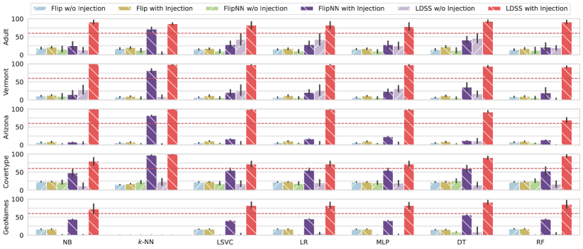
Figure 4. Prediction accuracy (%) of trigger samples for models trained with and without injection for all compared methods.

Evaluation Measures

We employ evaluation measures from digital model watermarking (Darvish Rouhani et al., 2019), focusing on leaked data detection performance. Given our black-box scenario without insights into training or model architecture, our assessment concentrates on prediction outcomes when querying the target model. We gauge the detection accuracy and standard deviation of trigger samples across seven conventional classification models: Naive Bayes (NB), $k$-Nearest Neighbor ($k$-NN), Linear Support Vector Classifier (LSVC), Logistic Regression (LR), Multi-Layer Perceptron (MLP), Decision Tree (DT), and Random Forest (RF). Ideally, models trained on the original dataset $\mathcal{D}_{orig}$ should have low trigger accuracy, while those on the modified dataset $\mathcal{D}_{mod}$ should score higher. The $k$-NN model is not evaluated for GeoNames as it is extremely slow.

Security is gauged via outlier and dense cluster detection, comparing the NN distance between original and injected samples rather than measuring the distribution changes in activation layers. Additionally, we assess fidelity through the train and test accuracy to ensure $\mathcal{D}_{mod}$ doesn’t drastically alter prediction accuracy.

Experiment Environment

All methods were written in Python 3.10. All experiments were conducted on a server with 24 CPUs of Intel^® Xeon^® E5-2620 v3 CPU @ 2.40 GHz, 64 GB memory, and one NVIDIA GeForce RTX 3090, running on Ubuntu 20.04.

Parameter Setting

In the experiments, we set the injection ratio $\rho$ to 10% of the training data size and $g=10$. For empty ball identification, we configure the contamination for Isolation Forest training at 0.05. During evaluation, the outlier percentage of injected samples is tested at contamination levels of 0.01, 0.05, and 0.1. Both $m$ and $k$ are fixed at 10. However, for features with fewer distinct values, the effective discretized values are less than $k$.

For each experiment, 11-fold cross-validation is conducted with a fixed random seed, where each round utilizes one fold as the training set and the next as the testing set. We first employ LDSS to generate both injection and trigger sets. Subsequently, we evaluate the classification models trained on the training set with/without the injection set. Afterward, we incrementally incorporate the remaining 9 folds of data into the training set. We then repeat the previously mentioned evaluations on these amalgamated datasets. This allows us to investigate the effectiveness of LDSS under the potential threat of dilution attacks.

4.2. Reliability and Robustness

We assess the reliability and robustness of LDSS by examining trigger accuracy across seven classification models. This is vividly depicted in Figure 4, which shows a consistent and pronounced difference in trigger accuracy for models trained on $\mathcal{D}_{orig}$ with or without LDSS synthetic injection. In contrast, Flip and FlipNN lack this clear differentiation across most models. The only exception is good performance demonstrated by FlipNN on $k$-NN model over all datasets. This is because FlipNN changes nearest neighbors of $g$ randomly selected samples to the same label and uses these label flipped samples directly as triggers. Hence, $k$-NN is much more likely to predict these triggers to the flipped label if it is trained after FlipNN modification. Given an accuracy threshold, e.g., $\tau=60\%$, one can confidently determine whether a target model was trained on the LDSS modified dataset. This determination is based on whether its trigger accuracy is above or below this threshold, especially considering the low standard deviation of trigger accuracy observed across all models and datasets.

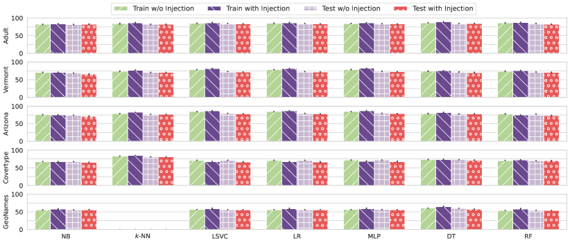
Figure 5. Train and test accuracy (%) with and without Synthetic Data Injection using LDSS.

4.3. Fidelity

Figure 5 shows that both train and test accuracy exhibit negligible deviation after the application of LDSS across all datasets and models, highlighted by the minimal standard deviation in accuracy variations. Specifically, the most significant accuracy variation among models is a mere 4.57%, which represents only about 6% relative deviation from the average testing accuracy (71.66%) of the Covertype dataset, as detailed in Table 4. This evidence justifies LDSS’s capacity to maintain fidelity across different model types. Thus, attackers are less likely to suspect that the dataset has been altered, enhancing the prospects of successful detection.

Table 4. Average accuracy (%), average difference (%), and maximum difference (%) when predicting hideout test dataset of different models trained on $\mathcal{D}_{orig}$ and $\mathcal{D}_{mod}$.

Datasets	Training			Testing
	Avg Acc.	Avg Diff.	Max Diff.	Avg Acc.	Avg Diff.	Max Diff.
Adult	84.95	1.90	3.23	86.84	0.86	2.00
Vermont	75.75	2.27	3.39	78.02	1.15	2.30
Arizona	80.78	2.63	3.59	82.35	1.39	3.68
Covertype	72.90	2.13	3.75	71.66	2.44	4.57
GeoNames	56.41	2.42	3.81	59.22	0.78	2.71

4.4. Security

We next explore potential detection and removal attacks aimed at identifying and eliminating the injected samples, which might allow subsequently trained models to bypass our detection mechanism. Under the realistic assumption that attackers lack detailed insights into local distributions or marginal statistics, they can only employ specific unsupervised methods to identify injected samples. We assess LDSS against two such methods: outlier detection and dense cluster detection. Moreover, we evaluate LDSS’s performance against dilution attacks.

Outlier Detection

Outlier detection is a straightforward yet effective method for identifying samples altered by data protection or watermarking techniques. Sometimes, a strategy might be overly aggressive in its attempt to optimize detection success, leading to changes that make affected samples too distant from the general population distribution. When this occurs, such samples become easy targets for outlier detection and can be readily removed by attackers. LDSS addresses this potential issue by ensuring that ball centers identified during empty ball generation (refer to Section 3.3) are not excessively distant from existing samples.

Figure 6(a) shows the outlier percentage of $\mathcal{D}_{inj}$ under various contamination settings using Isolation Forest (Liu et al., 2008). The percentage remains low, peaking at 55% even when the contamination reaches 0.1. Considering our injection ratio $\rho=10\%$, removing these outliers would also lead to discarding more genuine samples, thus compromising the accuracy of subsequently trained models.

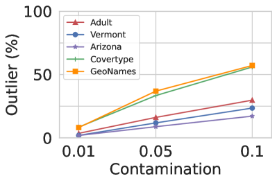
(a) Outlier (%) under different contamination settings without dilution.

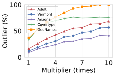
(b) Outlier (%) under different dilution multipliers (contamination = 0.05).

Figure 6. Outlier (%) found using Isolation Forest.

Dense Clusters Detection

While injected samples that are very similar and form dense clusters might be more effective in influencing the model, they are also more detectable. We assess this by evaluating the $k$-Nearest Neighbors distances ($k$-NN distances) and comparing them between original and injected samples.

As depicted in Figure 8, the $k$-NN distances of injected samples are consistently similar or even larger for a range of $k$ values from 1 to 10. These results indicate that LDSS does not synthesize very similar samples, enabling them to effectively evade dense cluster detection. Notably, the $k$-NN values for most injected samples overlap with the population in terms of both average and standard deviation.

Dilution Attack

LDSS has also been shown to be effective in situations where attackers dilute the leaked dataset by incorporating data from other sources within the same population. The aim is to reduce the influence of the injected samples, allowing the models trained on such data to evade detection. Our experiments consistently demonstrate LDSS’s ability to uphold high detection accuracy while preserving both fidelity and security.

As evident from Figure 7, the gap in trigger accuracy remains substantial. Even under the dilution of up to 10 times, the threshold of 60% distinctly separates the results across most models and datasets, underscoring the resilience of LDSS. Regarding fidelity, as the dataset becomes more diluted and injected samples comprise a smaller proportion, fidelity is expected to improve–a conclusion affirmed by Figure 9. In terms of security, it is anticipated that a greater proportion of injected samples will be identifiable via outlier detection as the dataset becomes more diluted. However, as shown in Figure 6(b), even under 10 times dilution, a minimum of 25% of injected samples remain undetected in 4 out of 5 datasets. Moreover, as dilution increases, it becomes less likely for injected samples to be flagged as dense clusters. Their $k$-NN distances are less apt to fall below those of genuine samples, both from the original and added datasets, as evident from Figure 10.

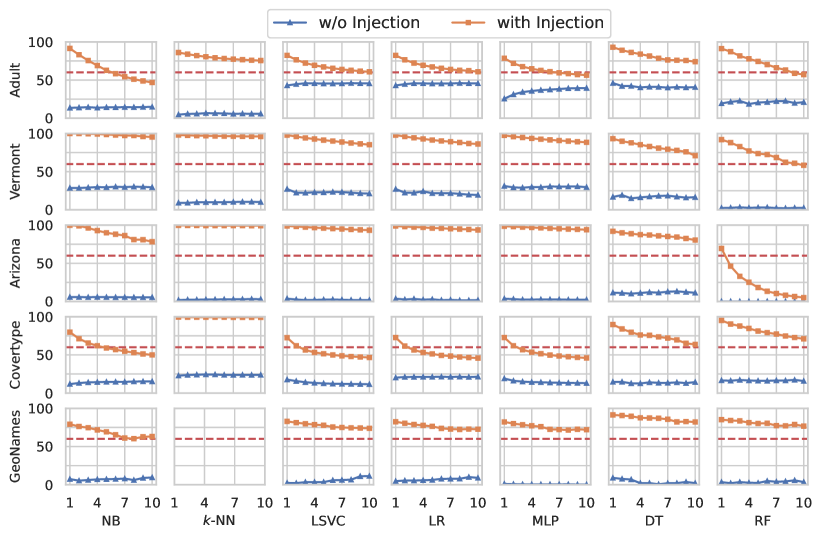
Figure 7. Prediction accuracy of trigger samples under different dilution multipliers for models trained with and without the injection using LDSS.

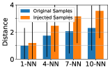
(a) Adult.

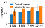
(b) Vermont.

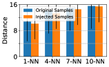
(c) Arizona.

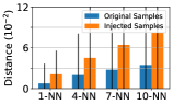
(d) Covertype.

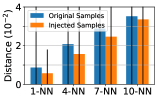
(e) GeoNames.

Figure 8. $1$-NN, $4$-NN, $7$-NN, and $10$-NN distances of original and injected samples in modified datasets.

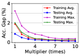
(a) Adult.

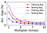
(b) Vermont.

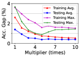
(c) Arizona.

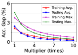
(d) Covertype.

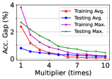
(e) GeoNames.

Figure 9. Train and test accuracy gap (%) under different dilution multipliers for models trained with and without the injection.

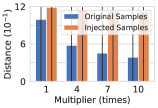
(a) Adult.

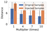
(b) Vermont.

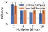
(c) Arizona.

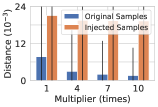
(d) Covertype.

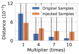
(e) GeoNames.

Figure 10. $k$-NN distances of original and injected samples under different dilution multipliers.

4.5. Efficiency

We measure the efficiency through the total execution time of the synthesis process. At a 10% injection ratio, LDSS synthesizes injection and trigger samples within 2 hours for the largest GeoNames dataset–1.5 hours for empty ball identification and around 30 minutes for sample synthesis. For the smallest Adult dataset, it takes just 30 minutes. Considering this is a one-time process per dataset, the duration is notably brief. It is important to mention that more time might be required for extensive parameter tuning and performance evaluation, especially since training multiple classification models can be time-consuming. There is room for further optimization, particularly in accelerating the slowest component: the Nearest Neighbor Search (NNS) during empty ball identification. The current implementation of LDSS utilizes FAISS (Johnson et al., 2021).

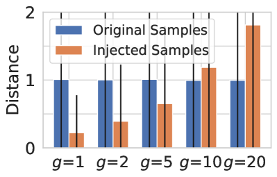
(a) Adult.

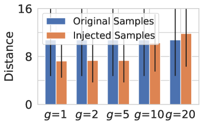
(b) Arizona.

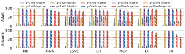
(c) Trigger Accuracy.

Figure 11. Comparison of $1$-NN distances and trigger accuracy under different $g$ values.

4.6. Parameter Study

There are two key parameters in LDSS: the number of empty balls, $g$, and the number of synthesized samples per ball, $h$. Instead of setting $g$ and $h$ directly, we first establish an injection ratio, $\rho$, from which we derive $h=\rho n/g$. When $\rho$ is fixed, it becomes imperative to choose $g$ wisely to maintain a balance between reliability and security. A smaller $g$ leads to closely clustered synthesized samples, while a larger $g$ reduces the influence of injected samples on the models. Our parameter study on the Adult and Arizona datasets, using a fixed injection ratio of 10%, showcases this balance. We vary $g$ from 1 to 20. Figures 11(a) and 11(b) indicate that smaller $g$ values (like 1, 2, or 5) yield smaller $1$-NN distances for injected samples relative to original samples. Concurrently, the accuracy of trigger samples after applying LDSS drops as $g$ rises. The optimal performance is observed at $g=10$.

A parameter study should be conducted to determine the ideal balance based on the injection ratio $\rho$. Figure 7 underscores the resilience of LDSS under dilution attack, illustrating that its efficacy remains intact even with a small $\rho$. Figure 10 indicates that the $1$-NN distance of injected samples is much larger than that of original samples when data is diluted, though the trigger accuracy also decreases. Thus, for lower $\rho$ values, decreasing $g$ could enhance detection rates without engendering overly dense clusters.

5. Related work

A plethora of research efforts have been devoted to safeguarding the Intellectual Property (IP) of machine learning models through watermarking techniques (Li et al., 2021; Xue et al., 2021; Boenisch, 2021; Zhang et al., 2020, 2021b; Fei et al., 2022; Peng et al., 2023; Quan et al., 2020; Wang and Wu, 2022). There are two broad categories of how watermark is embedded: either in training samples or directly in model parameters. Membership inference attack (Shokri et al., 2017) also serves as a straightforward method to ascertain whether a model has been trained on specific samples.

Embedding Watermark in Training Samples

Most methods employ a concept akin to model backdoors through data poisoning. The key concept is to train or finetune the target model with crafted samples either by modifying existing samples or via synthesis. Models are then trained to learn the specific pattern embedded with those crafted samples, either by mixing them into original training data or finetuning a trained model with only the crafted ones.

In (Zhang et al., 2018), samples are modified using label flipping, pixel patching, and noise addition. Adi et al. (2018) improved detection efficacy and watermark stealth by using multiple unrelated trigger batches. Li et al. (2020) enhanced patching with recent poisoning techniques (Chen et al., 2017; Gu et al., 2019), while Zhang et al. (2020) used a Unet (Ronneberger et al., 2015) to discreetly modify samples in images. Namba and Sakuma (2019) increased watermark persistence by setting exponentially higher weights to the crafted samples. Instead of altering training samples, Szyller et al. (2021) defended against model extraction by altering the predictions of selected samples in an additional API layer after model output. In (Wu et al., 2020; Qiao et al., 2023), the researchers adopted a similar strategy but focused on image-outputting models like GANs rather than classification models. In a related vein, other studies targeted time series models by adding trigger signals or words (Wang and Wu, 2022; Li et al., 2023).

Recent studies aim to enhance defense against potential watermark evasion or removal. Yang et al. (2021) improved the robustness against transformation attacks with a bi-level optimization, refining exemplar generation during training. Charette et al. (2022) used perturbation and retraining to embed a periodic pattern in model predictions, countering ensemble distillation. Meanwhile, Zhang et al. (2021a) improved upon (Zhang et al., 2020) by better aligning the added patch’s graphical details to the original image. Most such strategies focus on DNNs, which are usually over-parameterized and thereby capable of rich information being embedded. In LDSS, we use data synthesis similarly but without interacting with the training process. We adopt the straightforward label flipping approach, Flip, as our baseline. Drawing inspiration from (Adi et al., 2018; Namba and Sakuma, 2019), we enhanced Flip to FlipNN and designed LDSS to generate multiple samples in each empty ball, boosting watermark effectiveness.

Embedding Watermark in Model Parameters

Numerous studies (Song et al., 2017; Uchida et al., 2017; Wang et al., 2020) have concentrated on explicitly embedding watermark information into specific DNN layer parameters. Typically, these methods operate in a white-box setting during watermark verification or detection, requiring access to the model’s parameters or gradient information. Song et al. (2017) introduced various methods to encode bit information into model parameters using techniques like the least significant bit and sign encoding. On the other hand, Uchida et al. (2017) incorporated a bit string into convolution layers to induce a distribution bias. Detection is then facilitated by simply comparing the histogram of the parameter distribution with the targeted layer. Wang et al. (2020) further refined this approach using an auxiliary network to embed bit strings into selected convergent parameters, enhancing fidelity and robustness. As such, detection involves retrieving parameters or activation of specific layers in response to given inputs and comparing them to the embedded watermarks after decoding.

In many real-world scenarios, model detection operates in a black-box setting as models are usually accessed only as a service, returning predictions for given inputs. Thus, detecting watermarked models can only be performed by querying the target model with a specific trigger set to reveal the watermark in its predictions. This has led to advancements in model parameter embedding techniques to facilitate black-box detection. For example, Le Merrer et al. (2020) employs adversarial samples to alter decision boundaries so that the resulting model would classify them differently. These adversarial samples can be subsequently used as triggers to query a model for watermark detection. Chen et al. (2019) integrated binary signature strings into activation layers, categorizing them into two clusters. Each bit in the signature string corresponds to a cluster and links to specific key images. Detection is performed by querying the target model using these key images, decoding the resulting predictions into bits, and then comparing them with the original binary signature string. Similarly, Darvish Rouhani et al. (2019) embedded watermarks into rarely activated weights of selected layers. This modification ensures that the altered network yields different classifications for trigger inputs when compared to the original model.

While these methods typically offer greater accuracy and robustness compared to watermarking within training samples, they necessitate full control over the training process. Additionally, many demand white-box access to the model during detection. Our challenge concentrates on protecting data IP without predicting the attackers’ training methodologies, rendering this category of methods unsuitable for our purposes.

Membership Inference Attack

Membership inference attack provides a direct approach to detecting leaked data (Shokri et al., 2017). This technique assesses the likelihood that samples from the owner’s dataset have been used to train the target model, thereby identifying unauthorized usage. Nonetheless, this technique encounters challenges in discerning models trained on datasets with samples that are markedly similar or even identical to those in the owner’s collection. For instance, a patient may have medical records at multiple hospitals, and these records could be substantially identical. Furthermore, its accuracy may diminish when applied to shallow models (Truex et al., 2021) like $k$-NN, Logistic Regression, or shallow Decision Trees and MLPs. Such models are less likely to exhibit significant differences in individual samples if they are trained on independent datasets drawn from the same population.

6. Conclusion

In this paper, we emphasize the criticality of protecting a dataset’s IP, especially when it’s leaked and misused. To this end, we introduce LDSS, an innovative, model-oblivious technique designed for detecting leaked data. By seamlessly incorporating synthesized samples into the dataset, LDSS adeptly determines if a model has been trained on the modified dataset. Through rigorous experiments, our results consistently affirm the reliability, robustness, fidelity, security, and efficiency of LDSS in detecting leaked data across seven classification models.

More importantly, we advocate for dataset IP protection, moving away from the conventional emphasis on just model IP. We have significantly mitigated the overlooked risks of model releases based on unauthorized datasets, marking a pivotal shift in machine learning IP security considerations. Our approach particularly resonates when access is restricted to the model as a service.

References

- (1)
- Adi et al. (2018) Yossi Adi, Carsten Baum, Moustapha Cisse, Benny Pinkas, and Joseph Keshet. 2018. Turning Your Weakness into a Strength: Watermarking Deep Neural Networks by Backdooring. In USENIX Security. 1615–1631.
- Bellia (2011) Patricia L Bellia. 2011. WikiLeaks and the institutional framework for national security disclosures. Yale LJ 121 (2011), 1448.
- Bhatore et al. (2020) Siddharth Bhatore, Lalit Mohan, and Y Raghu Reddy. 2020. Machine learning techniques for credit risk evaluation: a systematic literature review. Journal of Banking and Financial Technology 4 (2020), 111–138.
- Bi et al. (2007) Ning Bi, Qiyu Sun, Daren Huang, Zhihua Yang, and Jiwu Huang. 2007. Robust Image Watermarking based on Multiband Wavelets and Empirical Mode Decomposition. TIP 16, 8 (2007), 1956–1966.
- Boenisch (2021) Franziska Boenisch. 2021. A Systematic Review on Model Watermarking for Neural Networks. Frontiers in Big Data 4 (2021), 729663.
- Charette et al. (2022) Laurent Charette, Lingyang Chu, Yizhou Chen, Jian Pei, Lanjun Wang, and Yong Zhang. 2022. Cosine model watermarking against ensemble distillation. In AAAI, Vol. 36. 9512–9520.
- Chawla et al. (2002) Nitesh V Chawla, Kevin W Bowyer, Lawrence O Hall, and W Philip Kegelmeyer. 2002. SMOTE: Synthetic Minority Over-Sampling Technique. JAIR 16 (2002), 321–357.
- Chen et al. (2019) Huili Chen, Bita Darvish Rouhani, and Farinaz Koushanfar. 2019. Blackmarks: Blackbox Multibit Watermarking for Deep Neural Networks. arXiv preprint arXiv:1904.00344 (2019).
- Chen et al. (2017) Xinyun Chen, Chang Liu, Bo Li, Kimberly Lu, and Dawn Song. 2017. Targeted Backdoor Attacks on Deep Learning Systems using Data Poisoning. arXiv preprint arXiv:1712.05526 (2017).
- Cheng et al. (2017) Long Cheng, Fang Liu, and Danfeng Yao. 2017. Enterprise data breach: causes, challenges, prevention, and future directions. Wiley Interdisciplinary Reviews: Data Mining and Knowledge Discovery 7, 5 (2017), e1211.
- Cox et al. (2007) Ingemar Cox, Matthew Miller, Jeffrey Bloom, Jessica Fridrich, and Ton Kalker. 2007. Digital Watermarking and Steganography. Morgan Kaufmann.
- Darvish Rouhani et al. (2019) Bita Darvish Rouhani, Huili Chen, and Farinaz Koushanfar. 2019. Deepsigns: An End-to-End Watermarking Framework for Ownership Protection of Deep Neural Networks. In ASPLOS. 485–497.
- Dua and Graff (2017) Dheeru Dua and Casey Graff. 2017. UCI Machine Learning Repository. http://archive.ics.uci.edu/ml
- Fei et al. (2022) Jianwei Fei, Zhihua Xia, Benedetta Tondi, and Mauro Barni. 2022. Supervised GAN Watermarking for Intellectual Property Protection. In IEEE International Workshop on Information Forensics and Security. 1–6.
- Gu et al. (2019) Tianyu Gu, Kang Liu, Brendan Dolan-Gavitt, and Siddharth Garg. 2019. Badnets: Evaluating backdooring attacks on deep neural networks. IEEE Access 7 (2019), 47230–47244.
- Halko et al. (2011) Nathan Halko, Per-Gunnar Martinsson, and Joel A Tropp. 2011. Finding Structure with Randomness: Probabilistic Algorithms for Constructing Approximate Matrix Decompositions. SIAM Rev. 53, 2 (2011), 217–288.
- Huang et al. (2000) Jiwu Huang, Yun Q Shi, and Yi Shi. 2000. Embedding Image Watermarks in DC Components. TCSVT 10, 6 (2000), 974–979.
- Huang et al. (2007) Yue Huang, Paul McCullagh, Norman Black, and Roy Harper. 2007. Feature selection and classification model construction on type 2 diabetic patients’ data. Artificial Intelligence in Medicine 41, 3 (2007), 251–262.
- Johnson et al. (2021) Jeff Johnson, Matthijs Douze, and Herve Jegou. 2021. Billion-Scale Similarity Search with GPUs. TBD 7, 3 (2021), 535–547.
- Knuth (2014) Donald E Knuth. 2014. The Art of Computer Programming: Seminumerical Algorithms, volume 2. Addison-Wesley Professional.
- Le Merrer et al. (2020) Erwan Le Merrer, Patrick Perez, and Gilles Trédan. 2020. Adversarial Frontier Stitching for Remote Neural Network Watermarking. Neural Computing and Applications 32, 13 (2020), 9233–9244.
- Lee et al. (2004) Jong-Seok Lee, Taeg-Sang Cho, Jiye Lee, Myung-Kee Jang, Tae-Kwang Jang, Dongkyung Nam, and Cheol Hoon Park. 2004. A Stochastic Search Approach for the Multidimensional Largest Empty Sphere Problem. (2004), 1–11.
- Li et al. (2023) Peixuan Li, Pengzhou Cheng, Fangqi Li, Wei Du, Haodong Zhao, and Gongshen Liu. 2023. PLMmark: a secure and robust black-box watermarking framework for pre-trained language models. In AAAI, Vol. 37. 14991–14999.
- Li et al. (2021) Yue Li, Hongxia Wang, and Mauro Barni. 2021. A Survey of Deep Neural Network Watermarking Techniques. Neurocomputing 461 (2021), 171–193.
- Li et al. (2020) Yiming Li, Ziqi Zhang, Jiawang Bai, Baoyuan Wu, Yong Jiang, and Shu-Tao Xia. 2020. Open-sourced Dataset Protection via Backdoor Watermarking. arXiv preprint arXiv:2010.05821 (2020).
- Liu et al. (2008) Fei Tony Liu, Kai Ming Ting, and Zhi-Hua Zhou. 2008. Isolation Forest. In ICDM. 413–422.
- Minka (2000) Thomas P Minka. 2000. Automatic Choice of Dimensionality for PCA. In NIPS. 577–583.
- Namba and Sakuma (2019) Ryota Namba and Jun Sakuma. 2019. Robust Watermarking of Neural Network with Exponential Weighting. In AsiaCCS. 228–240.
- Palaniappan and Mandic (2007) Ramaswamy Palaniappan and Danilo P Mandic. 2007. Biometrics from brain electrical activity: A machine learning approach. TPAMI 29, 4 (2007), 738–742.
- Peng et al. (2023) Sen Peng, Yufei Chen, Jie Xu, Zizhuo Chen, Cong Wang, and Xiaohua Jia. 2023. Intellectual Property Protection of DNN Models. World Wide Web 26, 4 (2023), 1877–1911.
- Potdar et al. (2005) Vidyasagar M Potdar, Song Han, and Elizabeth Chang. 2005. A Survey of Digital Image Watermarking Techniques. In IEEE International Conference on Industrial Informatics. 709–716.
- Qiao et al. (2023) Tong Qiao, Yuyan Ma, Ning Zheng, Hanzhou Wu, Yanli Chen, Ming Xu, and Xiangyang Luo. 2023. A novel model watermarking for protecting generative adversarial network. Computers & Security 127 (2023), 103102.
- Quan et al. (2020) Yuhui Quan, Huan Teng, Yixin Chen, and Hui Ji. 2020. Watermarking deep neural networks in image processing. TNNLS 32, 5 (2020), 1852–1865.
- Ribeiro et al. (2015) Mauro Ribeiro, Katarina Grolinger, and Miriam AM Capretz. 2015. Mlaas: Machine learning as a service. In IEEE 14th International Conference on Machine Learning and Applications. 896–902.
- Ronneberger et al. (2015) Olaf Ronneberger, Philipp Fischer, and Thomas Brox. 2015. U-net: Convolutional networks for biomedical image segmentation. In Medical Image Computing and Computer-Assisted Intervention. 234–241.
- Saha et al. (2020) Aniruddha Saha, Akshayvarun Subramanya, and Hamed Pirsiavash. 2020. Hidden trigger backdoor attacks. In AAAI, Vol. 34. 11957–11965.
- Shafahi et al. (2018) Ali Shafahi, W Ronny Huang, Mahyar Najibi, Octavian Suciu, Christoph Studer, Tudor Dumitras, and Tom Goldstein. 2018. Poison Frogs! Targeted Clean-label Poisoning Attacks on Neural Networks. In NeurIPS. 6106–6116.
- Sheikh et al. (2020) Mohammad Ahmad Sheikh, Amit Kumar Goel, and Tapas Kumar. 2020. An approach for prediction of loan approval using machine learning algorithm. In 2020 International Conference on Electronics and Sustainable Communication Systems. 490–494.
- Shklovski et al. (2014) Irina Shklovski, Scott D Mainwaring, Halla Hrund Skúladóttir, and Höskuldur Borgthorsson. 2014. Leakiness and creepiness in app space: Perceptions of privacy and mobile app use. In SIGCHI. 2347–2356.
- Shokri et al. (2017) Reza Shokri, Marco Stronati, Congzheng Song, and Vitaly Shmatikov. 2017. Membership Inference Attacks Against Machine Learning Models. In S&P. 3–18.
- Song et al. (2017) Congzheng Song, Thomas Ristenpart, and Vitaly Shmatikov. 2017. Machine Learning Models that Remember Too Much. In CCS. 587–601.
- Szyller et al. (2021) Sebastian Szyller, Buse Gul Atli, Samuel Marchal, and N Asokan. 2021. Dawn: Dynamic adversarial watermarking of neural networks. In MM. 4417–4425.
- Tipping and Bishop (1999) Michael E Tipping and Christopher M Bishop. 1999. Mixtures of Probabilistic Principal Component Analyzers. Neural Computation 11, 2 (1999), 443–482.
- Truex et al. (2021) Stacey Truex, Ling Liu, Mehmet Emre Gursoy, Lei Yu, and Wenqi Wei. 2021. Demystifying Membership Inference Attacks in Machine Learning As A Service. TSC 14, 06 (2021), 2073–2089.
- Uchida et al. (2017) Yusuke Uchida, Yuki Nagai, Shigeyuki Sakazawa, and Shin’ichi Satoh. 2017. Embedding watermarks into deep neural networks. In ICMR. 269–277.
- Wang et al. (2020) Jiangfeng Wang, Hanzhou Wu, Xinpeng Zhang, and Yuwei Yao. 2020. Watermarking in Deep Neural Networks via Error Back-Propagation. Electronic Imaging 2020, 4 (2020), 22–1.
- Wang and Wu (2022) Yumin Wang and Hanzhou Wu. 2022. Protecting the intellectual property of speaker recognition model by black-box watermarking in the frequency domain. Symmetry 14, 3 (2022), 619.
- Wu et al. (2020) Hanzhou Wu, Gen Liu, Yuwei Yao, and Xinpeng Zhang. 2020. Watermarking neural networks with watermarked images. TCSVT 31, 7 (2020), 2591–2601.
- Xue et al. (2021) Mingfu Xue, Yushu Zhang, Jian Wang, and Weiqiang Liu. 2021. Intellectual Property Protection for Deep Learning Models: Taxonomy, Methods, Attacks, and Evaluations. TAI 3, 6 (2021), 908–923.
- Yang et al. (2021) Peng Yang, Yingjie Lao, and Ping Li. 2021. Robust watermarking for deep neural networks via bi-level optimization. In ICCV. 14841–14850.
- Zhang et al. (2021a) Jie Zhang, Dongdong Chen, Jing Liao, Han Fang, Zehua Ma, Weiming Zhang, Gang Hua, and Nenghai Yu. 2021a. Exploring structure consistency for deep model watermarking. arXiv preprint arXiv:2108.02360 (2021).
- Zhang et al. (2020) Jie Zhang, Dongdong Chen, Jing Liao, Han Fang, Weiming Zhang, Wenbo Zhou, Hao Cui, and Nenghai Yu. 2020. Model Watermarking for Image Processing Networks. In AAAI, Vol. 34. 12805–12812.
- Zhang et al. (2021b) Jie Zhang, Dongdong Chen, Jing Liao, Weiming Zhang, Huamin Feng, Gang Hua, and Nenghai Yu. 2021b. Deep Model Intellectual Property Protection via Deep Watermarking. TPAMI 44, 8 (2021), 4005–4020.
- Zhang et al. (2018) Jialong Zhang, Zhongshu Gu, Jiyong Jang, Hui Wu, Marc Ph Stoecklin, Heqing Huang, and Ian Molloy. 2018. Protecting Intellectual Property of Deep Neural Networks with Watermarking. In AsiaCCS. 159–172.