$\bar{B}^{0}\to\bar{K}^{(*)\,0}X$, $B^{-}\to K^{(*)\,-}X$, $\bar{B}_{s}^{0}\to\eta(\eta^{\prime},\phi)X$ from the $X(3872)$ molecular perspective

Abstract

We study the decays $\bar{B}^{0}\to\bar{K}^{0}\,X$, $B^{-}\to K^{-}\,X$, $\bar{B}^{0}_{s}\to\eta(\eta^{\prime})\,X$, $\bar{B}^{0}\to\bar{K}^{*0}\,X$, $B^{-}\to K^{*-}\,X$ , $\bar{B}_{s}^{0}\to\phi\,X$, with $X\equiv X(3872)$, from the perspective of the $X(3872)$ being a molecular state made from the interaction of the $D^{*+}D^{-},D^{*0}\bar{D}^{0}$ and $c.c.$ components. We consider both the external and internal emission decay mechanisms and find an explanation for the $\bar{K}^{0}\,X$ and $K^{-}\,X$ production rates, based on the mass difference of the charged and neutral $D^{*}\bar{D}$ components. We also find that the internal and external emission mechanisms add constructively in the $\bar{B}^{0}\to\bar{K}^{0}\,X$, $B^{-}\to K^{-}\,X$ reactions, while they add destructively in the case of $\bar{B}^{0}\to\bar{K}^{*0}\,X$, $B^{-}\to K^{*-}\,X$ reactions. This feature explains the decay widths of the present measurements and allows us to make predictions for the unmeasured modes of $\bar{B}^{0}_{s}\to\eta(\eta^{\prime})\,X(3872)$ and $B^{-}\to K^{*-}\,X(3872)$. The future measurement of these decay modes will help us get a better perspective on the nature of the $X(3872)$ and the mechanisms present in production reactions of that state.

I Introduction

The $X(3872)$, as the first state found demanding an exotic, non $q\bar{q}$, nature, has been the subject of intense debate concerning its structure. Some groups claim a molecular nature with the $D^{*+}D^{-}$, $D^{*0}\bar{D}^{0}$ and c.c. components Braaten:2020nmc ; Liu:2020tqy ; Meng:2020cbk ; Dong:2021juy ; Wu:2021udi ; Gordillo:2021bra ; Dong:2021bvy ; Meng:2021kmi ; Kamiya:2022thy ; Lin:2022wmj ; Ji:2022uie ; Wang:2022qxe ; Wang:2022xga ; Kinugawa:2023fbf ; Yang:2023mov ; Wu:2023rrp ; Peng:2023lfw ; Terashima:2023tun , other groups claim a compact tetraquark state Shi:2021jyr ; Esposito:2021vhu ; Huang:2021poj ; Chen:2022ddj ; Sharma:2022ena , or some mixture of the two structures Lebed:2022vks ; Wang:2023ovj (see Refs. Kalashnikova:2018vkv ; Yamaguchi:2019vea ; Brambilla:2019esw ; Guo:2019twa ; Chen:2022asf ; Mai:2022eur for earlier related work). The extreme proximity of the state to the $D^{*0}\bar{D}^{0}$ threshold has been a main factor to support the molecular nature Guo:2017jvc ; Dong:2021juy , but, as discussed in detail in Ref. Song:2023pdq , the proximity of the state to a threshold is not sufficient to guarantee its molecular nature, although certainly makes it far more likely. It is found in Ref. Song:2023pdq that it is possible to have a state of non-molecular nature very close to a threshold, but one pays a huge price: the scattering length $a$ for the hadron-hadron components, to which the state inevitably couples, goes to zero, and the effective range $r_{0}$ goes to infinity in the limit of zero energy binding. With the small but finite binging of the $X(3872)$, the resulting $a,r_{0}$ magnitudes if one demands the state to be of non-molecular nature are very small and very large, respectively, compared with experimental data, to the point that one can exclude the non-molecular nature with uncertainties smaller than about $5\%$.

Very recently, in the work of Ref. ShenWang , the $\bar{B}^{0}\to\bar{K}^{0}\,X(3872)$ and $B^{-}\to K^{-}\,X(3872)$ reactions were proposed as a means to learn about the nature of the $X(3872)$. Indeed, with a compact tetraquark nature for the $X(3872)$, one expects the branching ratio of the two decay modes to be equal, but experimentally $\mathcal{B}(B^{-}\to K^{-}\,X(3872))/\mathcal{B}(\bar{B}^{0}\to\bar{K}^{0}\,X(3872))\simeq 2$. Instead, from the molecular perspective this ratio is tied to the loop functions $G_{i}$ for the neutral and charged components $D^{*0}\bar{D}^{0}$, $D^{*+}D^{-}$, respectively, which are different at the pole of the state because of the mass difference between the charged $D^{*+}D^{-}$ and neutral $D^{*0}\bar{D}^{0}$ components.

In Ref. ShenWang , the decay from the molecular perspective is studied considering the dominant external emission decay mode. In the present work we follow closely the idea of Ref. ShenWang but include in the study also the internal emission. Then extend the idea to study the $\bar{B}^{0}\to\bar{K}^{*0}\,X(3872)$, $B^{-}\to K^{*-}\,X(3872)$ and $\bar{B}^{0}_{s}\to\phi\,X(3872)$ decays. The latter reaction proceeds only via internal emission, and we would expect a small rate compared to that of the $\bar{B}^{0}\to\bar{K}^{*0}\,X(3872)$ decay, but, surprisingly, the rates are similar. Its explanation is found, because in the case of the $\bar{K}^{0},K^{-}$ pseudoscalar production the external and internal emission mechanisms add constructively, while in the case of $\bar{K}^{*0},K^{*-}$ production they add destructively. We compare ratios of branching ratios for presently measured decay modes and make predictions for the unmeasured modes, $\bar{B}^{0}_{s}\to\eta(\eta^{\prime})\,X(3872)$ and $B^{-}\to K^{*-}\,X(3872)$. It will be interesting to compare these predictions with future measurements, which will certainly help to go deeper in our understanding of the nature of the $X(3872)$ and the mechanisms of its production.

II Formalism

II.1 The molecular $X(3872)$ state

We follow here the work of Ref. Song:2023pdq , where the $X(3872)$ is obtained from the interaction of the $D^{*0}\bar{D}^{0},D^{*+}D^{-}$ ($+c.c.$) components. The extended local hidden gauge approach is used, with the coupled channels

$$\begin{split}X_{\rm c}=&\dfrac{1}{\sqrt{2}}(D^{*+}D^{-}-D^{*-}D^{+}),\\[5.69054pt] X_{\rm n}=&\dfrac{1}{\sqrt{2}}(D^{*0}\bar{D}^{0}-\bar{D}^{*0}D^{0}).\end{split}$$ (1)

The interaction between these components stems from the exchange of $\rho$ and $\omega$ vector mesons, and with the label $X_{\rm c}\equiv 1,X_{\rm n}\equiv 2$, one finds the interaction matrix

$$\centering V=\left(\begin{array}[]{cc}\tilde{v}&\tilde{v}\\ \tilde{v}&\tilde{v}\\ \end{array}\right),\@add@centering$$ (4)

with

$$\tilde{v}=-g^{2}\;\dfrac{4\,m_{D^{*0}}\,m_{D^{0}}}{M^{2}_{V}};~{}~{}~{}~{}g=\dfrac{M_{V}}{2\,f};~{}~{}~{}M_{V}=800\,\textrm{ MeV},~{}~{}~{}f=93\,\textrm{ MeV},$$ (5)

which has been calculated at the $D^{*0}\bar{D}^{0}$ threshold. The isospin states, with the isospin multiplets phase convention $(D^{+},-D^{0})$, $(\bar{D}^{0},D^{-})$ (and same for $D^{*}$), are given by

$$\begin{split}|X,I=0\rangle=\dfrac{1}{\sqrt{2}}\,(X_{\rm c}+X_{\rm n}),\\[5.69054pt] |X,I=1,I_{3}=0\rangle=\dfrac{1}{\sqrt{2}}\,(X_{\rm c}-X_{\rm n}),\end{split}$$ (6)

and we see that for $I=0$ the interaction is attractive and can produce a bound state, but for $I=1$ the interaction is zero and we do not expect a bound state. We note in passing that the strength of the interaction here is double than for $I=0$ in the $T_{cc}$ state FeijooLiang . This means we should expect a bigger binding for the $X(3872)$ than for the $T_{cc}$. With the centroid of mass data and the $X(3872)$ mass of the PDG pdg , which we write below,

$$m_{{D}^{0}}=(1864.84\pm 0.05)\,\textrm{ MeV}, m_{{D}^{+}}=(1869.66\pm 0.05)\,\textrm{ MeV},$$

$$m_{D^{*0}}=(2006.85\pm 0.05)\,\textrm{ MeV}, m_{D^{*+}}=(2010.26\pm 0.05)\,\textrm{ MeV},$$ (7)

$$m_{D^{*0}}+m_{{D}^{0}}=3871.69\,\textrm{ MeV}, m_{D^{*+}}+m_{{D}^{-}}=3879.92\,\textrm{ MeV},$$

$$M_{X(3872)}=(3871.65\pm 0.06)\,\textrm{ MeV},$$

the binding of the $X(3872)$ with respect to the $D^{*0}\bar{D}^{0}$ threshold is of $0.04\,\textrm{ MeV}$, but can be larger considering the uncertainties of the masses.

The scattering matrix with this potential is easily obtained as

$$\centering T=[1-VG]^{-1}\,V=\dfrac{1}{\rm det}\;\left(\begin{array}[]{cc}\tilde{v}&\tilde{v}\\ \tilde{v}&\tilde{v}\\ \end{array}\right),\@add@centering$$ (10)

with det being the determinant of $[1-VG]$, given by

$${\rm det}=1-\tilde{v}\,G_{1}-\tilde{v}\,G_{2},$$ (11)

and the diagonal $D^{*}\bar{D}$ loop function $G={\rm diag}[G_{1},G_{2}]$ given with the cutoff regularization by

$$G_{i}=\int_{|\vec{q}\,|<q_{\rm max}}\dfrac{{\rm d}^{3}q}{(2\pi)^{3}}\;\dfrac{\omega_{1}^{(i)}(\vec{q}\,)+\omega_{2}^{(i)}(\vec{q}\,)}{2\,\omega_{1}^{(i)}(\vec{q}\,)\,\omega_{2}^{(i)}(\vec{q}\,)}\;\dfrac{1}{s-[\omega_{1}^{(i)}(\vec{q}\,)+\omega_{2}^{(i)}(\vec{q}\,)]^{2}+i\epsilon},$$ (12)

with $\omega_{j}^{(i)}(\vec{q}\,)=\sqrt{m_{j}^{2}+\vec{q}^{\;2}}$ the energy of particle $j$ in the $i$-th channel. We use $q_{\rm max}=420\,\textrm{ MeV}$, as demanded in the study of the $T_{cc}$, with $D^{*}D$ components FeijooLiang , but to get the nominal binging of $40\,\rm keV$ we have to multiply $\tilde{v}$ by a factor $\beta=0.537$. Then we need to know the couplings of the $X(3872)$ to any of the charged or neutral components and we find

$$g_{1}^{2}=\lim_{s\to s_{0}}(s-s_{0})\,T_{11},~{}~{}~{}~{}~{}g_{1}g_{2}=\lim_{s\to s_{0}}(s-s_{0})\,T_{12},$$ (13)

with $s_{0}$ the squared of the energy of the $X(3872)$ state. From Eqs. (10) and (11) using l’Hospital rule for the limit, we find

$$g_{1}^{2}=\dfrac{\tilde{v}}{-\tilde{v}\frac{\partial}{\partial s}\,(G_{1}+G_{2})}=g_{1}\,g_{2}.$$ (14)

This means that $g_{1}=g_{2}$ (or $g_{\rm c}=g_{\rm n}$ in the nomencluture for charged or neutral components). In the formalism below we just need $G_{1},G_{2}$ at $s_{0}$ and the ratio $g_{\rm n}/g_{\rm c}=1$, which indicates that we have an $I=0$ state.

The formalism that we use here follows closely the one of Ref. ShenWang to study the $\bar{B}^{0}\to\bar{K}^{0}\,X(3872)$ and $B^{-}\to K^{-}\,X(3872)$ decays. In addition we include the hadronization from the internal emission mode and extend the formalism to the production of vector mesons.

II.2 Internal emission for pseudoscalar production

From the molecular point of view, the $X(3872)$ is given by

$$X=\dfrac{1}{\sqrt{2}}(X_{\rm c}+X_{\rm n}),$$ (15)

where $X_{\rm c}$ and $X_{\rm n}$ are the charged and neutral components of $D\bar{D}^{*},\bar{D}D^{*}$ respectively, shown in Eq. (1). Altogether

$$X=\dfrac{1}{2}(D^{*+}D^{-}-D^{*-}D^{+}+D^{*0}\bar{D}^{0}-\bar{D}^{*0}D^{0}),$$ (16)

which has isospin $I=0$ and $C$-parity $C=+$. In $s$-wave this state corresponds to $J^{P}=1^{+}$, completing the quantum numbers of the state.

At the quark level, the weak decay for $\bar{B}^{0}\to\bar{K}^{0}\,X(3872)$ and $B^{-}\to K^{-}\,X(3872)$ proceeds as shown in Fig. 1.

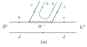
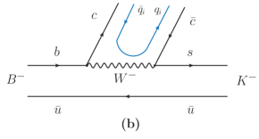
Figure 1: Internal emission mechanism at the quark level for $\bar{B}^{0}\to\bar{K}^{0}\,c\bar{c}$ decay (a) and $B^{-}\to K^{-}\,c\bar{c}$ decay (b).

The $X(3872)$ production from these mechanism is accomplished by means of hadronization of the $c\bar{c}$ component. Let us see how this proceeds. We start by writing the pseudoscalar ($P$) and vector ($V$) matrices for $q_{i}\bar{q}_{j}$ in terms of the physical mesons. With the $\eta,\eta^{\prime}$ mixing of Ref. Bramon , we have

$$P=\left(\begin{array}[]{cccc}\frac{1}{\sqrt{2}}\pi^{0}+\frac{1}{\sqrt{3}}\eta+\frac{1}{\sqrt{6}}\eta^{\prime}&\pi^{+}&K^{+}&\bar{D}^{0}\\[5.69054pt] \pi^{-}&-\frac{1}{\sqrt{2}}\pi^{0}+\frac{1}{\sqrt{3}}\eta+\frac{1}{\sqrt{6}}\eta^{\prime}&K^{0}&D^{-}\\[5.69054pt] K^{-}&\bar{K}^{0}&~{}-\frac{1}{\sqrt{3}}\eta+\sqrt{\frac{2}{3}}\eta^{\prime}{}&D_{s}^{-}\\[5.69054pt] D^{0}&D^{+}&D_{s}^{+}&\eta_{c}\\ \end{array}\right),$$ (17)

$$V=\left(\begin{array}[]{cccc}\frac{1}{\sqrt{2}}\rho^{0}+\frac{1}{\sqrt{2}}\omega&\rho^{+}&K^{*+}&\bar{D}^{*0}\\[5.69054pt] \rho^{-}&-\frac{1}{\sqrt{2}}\rho^{0}+\frac{1}{\sqrt{2}}\omega&~{}K^{*0}{}&D^{*-}\\[5.69054pt] K^{*-}&\bar{K}^{*0}&\phi&D_{s}^{*-}\\[5.69054pt] D^{*0}&D^{*+}&D_{s}^{*+}&J/\psi\\ \end{array}\right).$$ (18)

Then, upon hadronization of the $c\bar{c}$, we need to create a vector and a pseudoscalar, but the order matters and we can have $PV$ or $VP$ combinations. Hence

$${\rm a)}~{}PV:~{}~{}c\bar{c}\to\sum_{i}c\,\bar{q}_{i}q_{i}\,\bar{c}=\sum_{i}P_{4i}\,V_{i4}=(PV)_{44}=D^{0}\bar{D}^{*0}+D^{+}D^{*-}\,+\cdots,$$ (19)

$${\rm b)}~{}VP:~{}~{}c\bar{c}\to\sum_{i}c\,\bar{q}_{i}q_{i}\,\bar{c}=\sum_{i}V_{4i}\,P_{i4}=(VP)_{44}=D^{*0}\bar{D}^{0}+D^{*+}D^{-}\,+\cdots,$$ (20)

where the notation “$\cdots$” indicates other terms that have no overlap with the $X(3872)$ components of Eq. (16). We see that the combination $(VP)_{44}-(PV)_{44}$,

$$(VP)_{44}-(PV)_{44}=D^{*+}D^{-}+D^{*0}\bar{D}^{0}-D^{*-}D^{+}-\bar{D}^{*0}D^{0},$$ (21)

has a perfect match with Eq. (16). This hadronization is common to $\bar{B}^{0}\to\bar{K}^{0}\,X(3872)$ and $B^{-}\to K^{-}\,X(3872)$.

Let us see with the same mechanism, how we can have the decay $\bar{B}_{s}^{0}\to\eta(\eta^{\prime})\,X(3872)$. The mechanism is shown in Fig. 2.

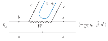
Figure 2: Internal emission mechanism at the quark level for $\bar{B}_{s}^{0}\to\eta(\eta^{\prime})\,c\bar{c}$ decay.

The hadronization in this case gives us the same combination as in Eq. (21), and the $s\bar{s}$ splits into $\eta$ and $\eta^{\prime}$ according to the matrix element $P_{33}$ of Eq. (17), as

$$s\bar{s}\to-\frac{1}{\sqrt{3}}\,\eta+\sqrt{\frac{2}{3}}\,\eta^{\prime}.$$ (22)

II.3 External emission for pseudoscalar production

External emission is the dominant mode of weak decay Chau since it is color favoured. One expects something like a factor $3$ times bigger amplitude than for internal emission. The mechanism for external emission is depicted in Fig. 3.

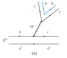
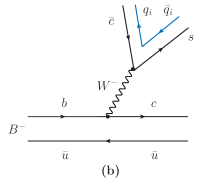
Figure 3: External emission mechanism for $\bar{B}^{0}\to\bar{c}s\,c\bar{d}$ decay (a) and $B^{-}\to\bar{c}s\,c\bar{u}$ decay (b).

Upon hadronization, we have three possibilities,

• $\bar{c}s\to PV,~{}c\bar{d}\to P\;(D^{+})$:

  $$s\bar{c}\to\sum_{i}s\,\bar{q}_{i}q_{i}\,\bar{c}=\sum_{i}P_{3i}\,V_{i4}=(PV)_{34}.$$ (23)

  Hence,

  $$\bar{c}s\,c\bar{d}\to(K^{-}D^{*0}+\bar{K}^{0}D^{*-}+\cdots)\,D^{+}.$$ (24)

• $\bar{c}s\to VP,~{}c\bar{d}\to P\;(D^{+})$:

  $$s\bar{c}\to\sum_{i}s\,\bar{q}_{i}q_{i}\,\bar{c}=\sum_{i}V_{3i}\,P_{i4}=(VP)_{34}.$$ (25)

  Hence,

  $$\bar{c}s\,c\bar{d}\to(K^{*-}\bar{D}^{0}+\bar{K}^{*0}D^{-}+\cdots)\,D^{+}.$$ (26)

• $\bar{c}s\to PP,~{}c\bar{d}\to V\;(D^{*+})$:

  $$s\bar{c}\to\sum_{i}s\,\bar{q}_{i}q_{i}\,\bar{c}=\sum_{i}P_{3i}\,P_{i4}=(PP)_{34}.$$ (27)

  Hence,

  $$\bar{c}s\,c\bar{d}\to(K^{-}\bar{D}^{0}+\bar{K}^{0}D^{-}+\cdots)\,D^{*+}.$$ (28)

We can see that the combination $(PP)_{34}\,D^{*+}-(PV)_{34}\,D^{+}$,

$$(PP)_{34}\,D^{*+}-(PV)_{34}\,D^{+}=(D^{*+}D^{-}-D^{*-}D^{+})\,\bar{K}^{0},$$ (29)

has again perfect overlap with the wave function of Eq. (16).

We can repeat the procedure for $K^{-}$ production of Fig. 3(b) and we find again

$$(PP)_{34}\,D^{*0}-(PV)_{34}\,D^{0}=(D^{*0}\bar{D}^{0}-\bar{D}^{*0}D^{0})\,\bar{K}^{-},$$ (30)

which overlaps with Eq. (16) in the same way.

We should also note that with this decay mode we find no terms that go to $\eta(\eta^{\prime})\,X(3872)$. Hence, $\eta,\eta^{\prime}$ production proceeds only via internal emission.

So far we have done the direct production of the components of the $X(3872)$. In order to produce the resonance, these components must propagate as depicted in Fig. 4,

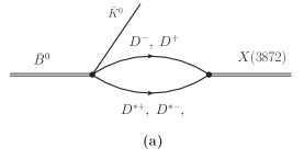
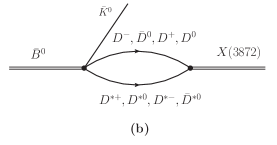
Figure 4: Propagation of $D\bar{D}^{*},\bar{D}D^{*}$ components to create the $X(3872)$: (a) external emission; (b) internal emission.

where the loops stand for the $G$ function of $D\bar{D}^{*}+c.c.$ propagation. Then we obtain the amplitude for $\bar{B}^{0}\to\bar{K}^{0}\,X(3982)$ as

$$t(\bar{K}^{0}) = C\,G_{D^{*+}D^{-}}(M_{X})\,g_{\rm c}+A\,\left[G_{D^{*+}D^{-}}(M_{X})\,g_{\rm c}+G_{D^{*0}\bar{D}^{0}}(M_{X})\,g_{\rm n}\right]$$ (31)

$$= C\,g_{\rm c}\,\left\{G_{D^{*+}D^{-}}(M_{X})+A^{\prime}\left[G_{D^{*+}D^{-}}(M_{X})+\frac{g_{\rm n}}{g_{\rm c}}\,G_{D^{*0}\bar{D}^{0}}(M_{X})\right]\right\},$$

where $A^{\prime}\equiv A/C$ and $g_{\rm c},g_{\rm n}$ are the couplings of $(D^{*+}D^{-}-D^{*-}D^{+})$ and $(D^{*0}\bar{D}^{0}-\bar{D}^{*0}D^{0})$ to $X(3872)$ of Eq. (16), respectively.

Similarly, for $K^{-}(\eta,\eta^{\prime})$ production we find

$$t(K^{-}) = C\,g_{\rm c}\,\left\{\frac{g_{\rm n}}{g_{\rm c}}\,G_{D^{*0}\bar{D}^{0}}(M_{X})+A^{\prime}\left[G_{D^{*+}D^{-}}(M_{X})+\frac{g_{\rm n}}{g_{\rm c}}\,G_{D^{*0}\bar{D}^{0}}(M_{X})\right]\right\},$$ (32)

$$t(\eta) = C\,g_{\rm c}\,A^{\prime}\left[G_{D^{*+}D^{-}}(M_{X})+\frac{g_{\rm n}}{g_{\rm c}}\,G_{D^{*0}\bar{D}^{0}}(M_{X})\right]\,(-\frac{1}{\sqrt{3}}),$$ (33)

$$t(\eta^{\prime}) = C\,g_{\rm c}\,A^{\prime}\left[G_{D^{*+}D^{-}}(M_{X})+\frac{g_{\rm n}}{g_{\rm c}}\,G_{D^{*0}\bar{D}^{0}}(M_{X})\right]\,(\sqrt{\frac{2}{3}}).$$ (34)

Experimentally $\Gamma(K^{-})/\Gamma(K^{0})\sim 2$ pdg and now we can see qualitatively the reason for this factor, because at the pole $(G_{D^{*0}\bar{D}^{0}}/G_{D^{*+}D^{-}})^{2}\sim 2$, as can be seen in the work of Ref. Gamermann , due to the mass difference between the $D^{*+}D^{-}$ and $D^{*0}\bar{D}^{0}$ components. Assuming the contribution of internal emission small, this could give a qualitative explanation of the experimental ratio, which is the idea of Ref. ShenWang . We aim at being more quantitative here and also extend the formalism to the production of vector mesons that we address below.

II.4 Internal emission for vector production

We now look at the reactions $\bar{B}^{0}\to\bar{K}^{*0}\,X(3872)$, $B^{-}\to K^{*-}\,X(3872)$, $\bar{B}_{s}^{0}\to\phi\,X(3872)$. The internal emission for vector production is identical to the one exposed before in Figs. 1(a) and 1(b), replacing $\bar{K}^{0}$ by $\bar{K}^{*0}$ and $K^{-}$ by $K^{*-}$ respectively. For $\phi$ production, it is also easy since the mechanism is the one of Fig. 2, where now $s\bar{s}\to\phi$. The weight $A$ will now be $\tilde{A}$, since the coupling of the $q\bar{q}$ component to pseudoscalars or vectors have different weights LiangOset .

II.5 External emission for vector production

Following the steps of the former subsection for external emission we find now

• $\bar{K}^{*0}$ production:

  $$(VV)_{34}\,D^{+}-(VP)_{34}\,D^{*+}~{}\to~{}(-1)(D^{*+}D^{-}-D^{*-}D^{+})\,\bar{K}^{*0};$$ (35)

• $K^{*-}$ production:

  $$(VV)_{34}\,D^{0}-(VP)_{34}\,D^{*0}~{}\to~{}(-1)(D^{*0}\bar{D}^{0}-\bar{D}^{*0}D^{0})\,K^{*-}.$$ (36)

Note that we obtain the same expression as in Eqs. (29) and (30), simply replacing $\bar{K}^{0}$ by $\bar{K}^{*0}$ and $K^{-}$ by $K^{*-}$ respectively. There is only one difference which is the sign. This different sign will be of relevance for the different rates obtained for pseudoscalar and vector production, as we shall see.

All this said, the amplitudes for vector production are now

$$t(\bar{K}^{*0}) = \tilde{C}\,g_{\rm c}\,\left\{-G_{D^{*+}D^{-}}(M_{X})+\tilde{A}^{\prime}\left[G_{D^{*+}D^{-}}(M_{X})+\frac{g_{\rm n}}{g_{\rm c}}\,G_{D^{*0}\bar{D}^{0}}(M_{X})\right]\right\},$$ (37)

$$t(K^{*-}) = \tilde{C}\,g_{\rm c}\,\left\{-\frac{g_{\rm n}}{g_{\rm c}}\,G_{D^{*0}\bar{D}^{0}}(M_{X})+\tilde{A}^{\prime}\left[G_{D^{*+}D^{-}}(M_{X})+\frac{g_{\rm n}}{g_{\rm c}}\,G_{D^{*0}\bar{D}^{0}}(M_{X})\right]\right\},$$ (38)

$$t(\phi) = \tilde{C}\,g_{\rm c}\,\tilde{A}^{\prime}\left[G_{D^{*+}D^{-}}(M_{X})+\frac{g_{\rm n}}{g_{\rm c}}\,G_{D^{*0}\bar{D}^{0}}(M_{X})\right],$$ (39)

where $\tilde{A}^{\prime}\equiv\tilde{A}/\tilde{C}$.

Note that in Eqs. (31) to (34) and here in Eqs. (37) to (39) the constants $\tilde{C}$ and $C$ are different, hence we cannot relate pseudoscalar production and vector production, but we can compare different rates for pseudoscalar production and different rates for vector production. There is one more thing, while $C$ and $\tilde{C}$ and $A,\tilde{A}$ are different, the ratio $A^{\prime}\equiv A/C$ and $\tilde{A}^{\prime}\equiv\tilde{A}/\tilde{C}$ indicates the fraction of internal to external emission, and this is basically related to the color factor. Hence we shall make the reasonable assumption that $A^{\prime}\equiv\tilde{A}^{\prime}$.

In addition, for angular momentum conservation we have the extra factor $p_{B_{(s)}}^{\mu}\,\epsilon_{\mu}(X)$ for pseudoscalar decay ShenWang and $\epsilon_{\mu}(V)\,\epsilon^{\mu}(X)$ for vector decay. Upon squaring the $t_{i}$ amplitudes, $|t_{i}|^{2}$, and summing over polarizations, the first term for pseudoscalar production gives $\vec{p}_{X}^{\;2}\,M_{B_{(s)}}^{2}/M_{X}^{2}$ and the second term for vector production a constant. Since $|\vec{p}_{X}|\equiv|\vec{p}_{P}|$ in the rest frame of $B_{(s)}$, with $\vec{p}_{P}$ the pseudoscalar momentum, for calculating ratios we just include the $\vec{p}_{P}^{\;2}$ factor in the formula of the width.

III Results

In Eqs. (31) to (39) we have the amplitudes for each one of the transitions considered. The decay width corresponding to these amplitudes are

$$\Gamma_{i\to j}=\dfrac{1}{8\pi}\;\dfrac{1}{M^{2}_{B_{i}}}\;|t_{i,j}|^{2}\,p_{j}\,F(p_{j}),$$ (40)

with

$$p_{j}=\dfrac{\lambda^{1/2}(M^{2}_{B_{i}},m^{2}_{j},M^{2}_{X})}{2\,M_{B_{i}}},$$ (41)

where $B_{i}$ is the decaying $B_{(s)}$ meson and $j$ the pseudoscalar or vector produced in addition to the $X(3872)$. The factor $F(p_{j})$, where a constant factor, inoperative in ratios, is omitted is

$$F(p_{j})=\left\{\begin{array}[]{ll}p_{j}^{2},&{\rm for~{}pseudoscalar~{}production};\\[2.84526pt] 1,&{\rm for~{}vector~{}production}.\\ \end{array}\right.$$ (44)

When calculating ratios between pseudoscalar or vector production rates, the factors $C\,g_{\rm c}$ and $\tilde{C}\,g_{\rm c}$ cancel and the ratios depend on the only parameter $A^{\prime}\equiv\tilde{A}^{\prime}$. The present experimental situation, according to the PDG pdg , is the following:

$$\mathcal{B}(\bar{B}^{0}\to\bar{K}^{0}\,X(3872)) = (1.1\pm 0.4)\times 10^{-4},$$

$$\mathcal{B}(B^{-}\to K^{-}\,X(3872)) = (2.1\pm 0.7)\times 10^{-4},$$

$$\mathcal{B}(\bar{B}^{0}\to\bar{K}^{*0}\,X(3872)) = (1.0\pm 0.5)\times 10^{-4},$$ (45)

$$\mathcal{B}(B^{-}\to K^{*-}\,X(3872)) < 6\times 10^{-4},$$

$$\mathcal{B}(\bar{B}_{s}^{0}\to\phi\,X(3872)) = (1.1\pm 0.4)\times 10^{-4}.$$

We determine the value of $A^{\prime}$ to get the ratio between $\mathcal{B}(\bar{B}^{0}_{s}\to\phi\,X)/\mathcal{B}(\bar{B}^{0}\to\bar{K}^{*0}\,X)$ and then the rest of the ratios are predictions. We find

$$A^{\prime}=0.2,$$ (46)

which makes sense as the color suppressed internal emission versus external emission modes. Then we find the ratios of Tables 1 and 2.

Table 1: Ratios of $R\equiv\mathcal{B}(B_{i}\to j)/\mathcal{B}(\bar{B}^{0}\to\bar{K}^{0}\,X(3872))$. The different life times $\tau_{B_{i}}$ are considered. In brackets experimental ratio with errors summed in quadrature.

	$B^{-}\to K^{-}\,X$	$\bar{B}_{s}^{0}\to\eta\,X$	$\bar{B}_{s}^{0}\to\eta^{\prime}\,X$
$R$	$2.07~{}~{}(1.91\pm 0.94)$	$0.043$	$0.048$

Table 2: Ratios of $R^{\prime}\equiv\mathcal{B}(B_{i}\to j)/\mathcal{B}(\bar{B}^{0}\to\bar{K}^{*0}\,X(3872))$. The different life times $\tau_{B_{i}}$ are considered. In brackets experimental ratio with errors summed in quadrature.

	$B^{-}\to K^{*-}\,X$	$\bar{B}_{s}^{0}\to\phi\,X$
$R^{\prime}$	$5.2~{}~{}(<6)$	$1.10~{}~{}(1.10\pm 0.68)$

The essential ingredient in understanding these results is the fact that $|G_{D^{*0}\bar{D}^{0}}|$ at the pole is bigger than $|G_{D^{*+}D^{-}}|$. $G_{D^{*+}D^{-}}$ looks like $G_{D^{*0}\bar{D}^{0}}$ but displaced about $7\;\textrm{ MeV}$ to the right, and both are negative. This has a consequence that $|G_{D^{*0}\bar{D}^{0}}|>|G_{D^{*+}D^{-}}|$ at the pole as can be seen in Fig. 5.

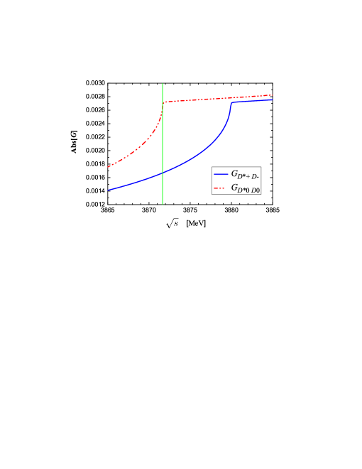
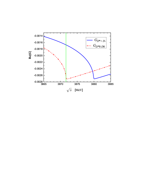
Figure 5: $G_{D^{*+}D^{-}}$ and $G_{D^{*0}\bar{D}^{0}}$ as a function of the energy $\sqrt{s}$. The vertical line indicates the mass of the $X(3872)$.

It is interesting to remark that the contribution of the internal emission, even if small, has been important to get these results. Indeed, if we neglect the internal emission then $\mathcal{B}(B^{-}\to K^{-}X)/\mathcal{B}(\bar{B}^{0}\to\bar{K}^{0}\,X)=2.5$, which is bigger than experiment. On the other hand, in this extreme case $\mathcal{B}(\bar{B}_{s}^{0}\to\phi X)=0$. The introduction of the internal emission term, adding constructively to the external emission in Eqs. (32) to (34), softens the former ratio. On the other hand, for vector production in Eqs. (37) and (38), the external and internal emissions interfere destructively for $\bar{K}^{*0}$ and $K^{*-}$ production, reducing their widths, and has a consequence that the rates of $\bar{B}^{0}\to\bar{K}^{*0}\,X(3872)$ and $\bar{B}_{s}^{0}\to\phi\,X(3872)$ are similar.

IV Conclusions

In this work we have addressed the issue of $B$ decays to a pseudoscalar and the $X(3872)$ and a vector and $X(3872)$, from the perspective that the $X(3872)$ is a dynamically generated state from the $D\bar{D}^{*}+c.c.$ interaction in coupled channels. In particular we have studied the decays $\bar{B}^{0}\to\bar{K}^{0}\,X$, $B^{-}\to K^{-}\,X$, $\bar{B}^{0}_{s}\to\eta(\eta^{\prime})\,X$, $\bar{B}^{0}\to\bar{K}^{*0}\,X$, $B^{-}\to K^{*-}\,X$ , $\bar{B}_{s}^{0}\to\phi\,X$, with $X\equiv X(3872)$. We have seen that the production of the final states requires both the mechanism of external and internal emission. Although the internal emission mechanism is suppressed with respect to external emission by a color factor, we have seen that for the vector production the two terms interfere destructively, while they add constructively for pseudoscalar production. This has as a consequence that while $\eta$ and $\eta^{\prime}$ production, which proceed via internal emission, are small compared to $\bar{K}^{0}$ of $K^{-}$ production, which proceeds via the sum of the two mechanisms, $\phi$ production, which also proceeds via internal emission, has comparable strength to $K^{*}$ production, where both external and internal emission are at work but add destructively. The reason for an unexpected factor $2$ between $K^{-}$ and $\bar{K}^{0}$ production is traced back to the composite nature of the $X(3972)$ from the charged and neutral $X_{\rm c},X_{\rm n}$ of Eq. (1) and the mass difference between $D^{*+}\,D^{-}$ and $D^{*0}\bar{D}^{0}$. Indeed, the production of the $X(3872)$ requires the propagation of the $D^{*}\bar{D}$ components, which is accomplished by means of the loop $G$ functions. The one of the charged components is displaced about $7\,\textrm{ MeV}$ to higher energies, due to the mass difference between the charged and neutral components, and this has as a consequence that at the pole energy the ratio $|G_{\rm n}/G_{\rm c}|^{2}$ is about $2.5$ (see Fig. 5). This would be the ratio between $K^{-}$ and $\bar{K}^{0}$ production rates in the absence of internal emission. The contribution of internal emission reduces this factor to about $2$. This provides a natural explanation for this apparently strange ratio that naively one would expect to be of the order of unity. The fact that the rates of vector production also appear fine with the same framework adds extra support to this picture. In addition we have made predictions for $\eta$ and $\eta^{\prime}$ production in the pseudoscalar sector, and $K^{*-}$ in the vector sector. Future measurements of these decays widths should provide extra support for this picture.

- (1) E. Braaten, L. P. He and J. Jiang, Phys. Rev. D 103, no.3, 036014 (2021).
- (2) M. Z. Liu and L. S. Geng, Eur. Phys. J. C 81, no.2, 179 (2021).
- (3) L. Meng, B. Wang and S. L. Zhu, Sci. Bull. 66, 1288-1295 (2021).
- (4) X. K. Dong, F. K. Guo and B. S. Zou, Progr. Phys. 41, 65-93 (2021).
- (5) Q. Wu, D. Y. Chen and T. Matsuki, Eur. Phys. J. C 81, no.2, 193 (2021).
- (6) M. C. Gordillo, F. De Soto and J. Segovia, Phys. Rev. D 104, no.5, 054036 (2021).
- (7) X. K. Dong, F. K. Guo and B. S. Zou, Commun. Theor. Phys. 73, no.12, 125201 (2021).
- (8) L. Meng, G. J. Wang, B. Wang and S. L. Zhu, Phys. Rev. D 104, no.9, 094003 (2021).
- (9) Y. Kamiya, T. Hyodo and A. Ohnishi, Eur. Phys. J. A 58, no.7, 131 (2022).
- (10) Z. Y. Lin, J. B. Cheng and S. L. Zhu, [arXiv:2205.14628 [hep-ph]].
- (11) T. Ji, X. K. Dong, M. Albaladejo, M. L. Du, F. K. Guo and J. Nieves, Phys. Rev. D 106, no.9, 9 (2022).
- (12) Y. Wang, Q. Wu, G. Li, W. H. Qin, X. H. Liu, C. S. An and J. J. Xie, Phys. Rev. D 106, no.7, 074015 (2022).
- (13) H. N. Wang, L. S. Geng, Q. Wang and J. J. Xie, Chin. Phys. Lett. 40, no.2, 021301 (2023).
- (14) T. Kinugawa and T. Hyodo, [arXiv:2303.07038 [hep-ph]].
- (15) G. Yang, J. Ping and J. Segovia, Eur. Phys. J. C 83, no.8, 772 (2023).
- (16) Q. Wu, M. Z. Liu and L. S. Geng, [arXiv:2304.05269 [hep-ph]].
- (17) F. Z. Peng, M. J. Yan and M. Pavon Valderrama, [arXiv:2304.13515 [hep-ph]].
- (18) I. Terashima and T. Hyodo, Phys. Rev. C 108, no.3, 035204 (2023).
- (19) P. P. Shi, F. Huang and W. L. Wang, Phys. Rev. D 103, no.9, 094038 (2021).
- (20) A. Esposito, L. Maiani, A. Pilloni, A. D. Polosa and V. Riquer, Phys. Rev. D 105, no.3, L031503 (2022).
- (21) H. X. Huang, X. Jin, Y. Tan and J. L. Ping, EPL 135, no.3, 31001 (2021).
- (22) C. Chen, H. Chen, W. Q. Niu and H. Q. Zheng, Eur. Phys. J. C 83, no.1, 52 (2023).
- (23) A. Sharma and A. Upadhyay, [arXiv:2207.02456 [hep-ph]].
- (24) R. F. Lebed and S. R. Martinez, Phys. Rev. D 106, no.7, 074007 (2022).
- (25) G. J. Wang, Z. Yang, J. J. Wu, M. Oka and S. L. Zhu, [arXiv:2306.12406 [hep-ph]].
- (26) Y. S. Kalashnikova and A. V. Nefediev, Phys. Usp. 62, no.6, 568-595 (2019).
- (27) Y. Yamaguchi, A. Hosaka, S. Takeuchi and M. Takizawa, J. Phys. G 47, no.5, 053001 (2020).
- (28) N. Brambilla, S. Eidelman, C. Hanhart, A. Nefediev, C. P. Shen, C. E. Thomas, A. Vairo and C. Z. Yuan, Phys. Rept. 873, 1-154 (2020).
- (29) F. K. Guo, X. H. Liu and S. Sakai, Prog. Part. Nucl. Phys. 112, 103757 (2020).
- (30) H. X. Chen, W. Chen, X. Liu, Y. R. Liu and S. L. Zhu, Rept. Prog. Phys. 86, no.2, 026201 (2023).
- (31) M. Mai, U. G. Meißner and C. Urbach, Phys. Rept. 1001, 1-66 (2023).
- (32) F. K. Guo, C. Hanhart, U. G. Meißner, Q. Wang, Q. Zhao and B. S. Zou, Rev. Mod. Phys. 90, no.1, 015004 (2018); [erratum: Rev. Mod. Phys. 94, no.2, 029901 (2022)].
- (33) J. Song, L. R. Dai and E. Oset, [arXiv:2307.02382 [hep-ph]].
- (34) H. N. Wang, L. S. Geng, Q. Wang and J. J. Xie, Chin. Phys. Lett. 40, no.2, 021301 (2023).
- (35) A. Feijoo, W. H. Liang and E. Oset, Phys. Rev. D 104, no.11, 114015 (2021).
- (36) R. L. Workman et al. [Particle Data Group], Review of Particle Physics, Prog. Theor. Exp. Phys. 2022, 083C01 (2022).
- (37) A. Bramon, A. Grau and G. Pancheri, Phys. Lett. B 283, 416-420 (1992).
- (38) L. L. Chau, Phys. Rept. 95, 1-94 (1983).
- (39) D. Gamermann and E. Oset, Phys. Rev. D 80, 014003 (2009).
- (40) W. H. Liang and E. Oset, Eur. Phys. J. C 78, no.6, 528 (2018).