Finite element discretization of the steady, generalized Navier–Stokes equations with inhomogeneous Dirichlet boundary conditions

Abstract

We propose a finite element discretization for the steady, generalized Navier–Stokes equations for fluids with shear-dependent viscosity, completed with inhomogeneous Dirichlet boundary conditions and an inhomogeneous divergence constraint. We establish (weak) convergence of discrete solutions as well as a priori error estimates for the velocity vector field and the scalar kinematic pressure. Numerical experiments complement the theoretical findings.

35J60; 35Q35; 65N12; 65N15; 65N30; 76A05.

1 Introduction

The steady motion of a homogeneous, incompressible generalized Newtonian fluid can be modelled by the generalized Navier–Stokes equations

(1) $$-\textup{div}\,\bm{S}(\bm{Dv})+\textup{div}\,(\bm{v}\otimes\bm{v})+\nabla q=\bm{f}\quad\textrm{ in }\Omega\,.$$

Here, $\Omega\subseteq\mathbb{R}^{d}$, $d\in\{2,3\}$, denotes a bounded polyhedral Lipschitz domain, which is occupied by the fluid, and $\bm{f}\colon\Omega\to\mathbb{R}^{d}$ denotes an external body force. The velocity vector field $\bm{v}\colon\overline{\Omega}\to\mathbb{R}^{d}$ and the scalar kinematic pressure $q\colon\Omega\to\mathbb{R}$ are the unknowns. Moreover, we assume that the viscosity can be expressed as a function of the shear rate. Therefore, we consider an extra stress tensor $\bm{S}\colon\mathbb{R}^{d\times d}\to\mathbb{R}_{\textup{sym}}^{d\times d}$ that has $(p,\delta)$-structure (cf. Assumption 1). While the particular case $p=2$ results in the well-known Navier–Stokes equations for Newtonian fluids, the cases $p<2$ and $p>2$ correspond to shear-thinning and shear-thickening fluids, respectively.

The system is completed by the inhomogeneous Dirichlet boundary condition

(2) $$\bm{v} =\bm{g}_{2} \quad\textrm{ on }\partial\Omega\,,$$

and, for the sake of generality, the inhomogeneous divergence constraint

(3) $$\operatorname{div}\bm{v} =g_{1} \quad\textrm{ in }\Omega\,.$$

Several results have been established for finite element (FE) discretizations of the corresponding generalized Stokes system: in [4], error estimates are proved for homogeneous Dirichlet boundary conditions. Similar results have been established in [26] for fluids with shear-rate- and pressure-dependent viscosity, $p<2$, and mixed inhomogeneous boundary conditions. To the best of the authors’ knowledge, FE discretizations for the system (1)–(3) have solely been investigated in the case of homogeneous Dirichlet boundary conditions as well as merely (weak) convergence results has been established. This was done in a fairly general context, e.g., for implicitly constituted fluids and unsteady flows thereof (cf. [14, 45]). In a recent series of articles, a local discontinuous Galerkin (LDG) scheme for the system (1)–(3) has been proposed in the case $p>2$.Existence and (weak) convergence results have been derived (cf. [30]) as well as a priori error estimates in the case of homogeneous Dirichlet boundary conditions (cf. [31, 32]).

In this work, we provide a FE discretization for the fully inhomogeneous, steady system (1)–(3). Then, for this FE discretization, we establish its well-posedness (i.e., existence of discrete solutions), stability (i.e., a priori energy bounds), convergence (i.e., (weak) convergence towards a solution of an appropriate weak formulation of the system (1)–(3)), as well as a priori error estimates.

While most of our assumptions (like existence of a Fortin interpolation operator) are rather uncritical, we require certain smallness constraints for the following reasons: in the shear-thickening and in the homogeneous case, the corresponding operator is coercive and, thus, existence of weak solutions can be proved with the theory of pseudo-monotone operators (and, additionally, the Lipschitz truncation method if $p\leq\tfrac{3d}{d+2}$) (cf. [37, 35, 21, 16]). Furthermore, the existence of weak solutions is only known under additional assumptions like smallness of the data $g_{1}$ and $\bm{g_{2}}$ (cf. [34, 27, 22, 33, 7, 29]). This transfers to the discrete situation: if $p\leq 2$, then we require smallness of the data $g_{1}$ and $\bm{g_{2}}$, in order to show the existence and (weak) convergence of discrete solutions. In addition, because of quadratic terms coming from the convective term $\textup{div}\,(\bm{v}\otimes\bm{v})$,the error estimate for the velocity requires smallness of the solution $\bm{v}$ in any case. To the best of the authors’ knowledge, this corresponds to the state of the art regarding error estimates for the (much more intensively researched) classical Navier–Stokes equations.

This paper is structured as follows: In Section 2, we introduce the needed notation, the finite element setting and precise formulations of continuous and discrete problem. Then, Section 3 is dedicated to the well-posedness, stability and (weak) convergence of the discrete formulation. In Section 4, we derive a priori error estimates for the velocity vector field and the kinematic pressure. In Section 5, numerical experiments are carried out to complement the theoretical findings.

2 Preliminaries

In this section, we provide the needed notation for the analysis and give precise definitions of the continuous problem and a finite element discretization.

2.1 Notation

We employ $c,C>0$ to denote generic constants, that may change from line to line, but do not depend on the crucial quantities. Moreover, we write $u\sim v$ if and only if there exist constants $c,C>0$ such that $c\,u\leq v\leq C\,u$.

For $k\in\mathbb{N}$ and $p\in[1,\infty]$, we employ the customary Lebesgue spaces $(L^{p}(\Omega),\|\cdot\|_{p})$ and Sobolev spaces $(W^{k,p}(\Omega),\|\cdot\|_{k,p})$, where $\Omega\subseteq\mathbb{R}^{d}$, $d\in\{2,3\}$, is a bounded, polyhedral Lipschitz domain. The space $\smash{W^{1,p}_{0}(\Omega)}$ is defined as those functions from $W^{1,p}(\Omega)$ whose traces vanish on $\partial\Omega$. We equip $\smash{W^{1,p}_{0}(\Omega)}$ with the norm $\smash{\|\nabla\cdot\|_{p}}$. The conjugate exponent is denoted by $p^{\prime}=\tfrac{p}{p-1}\in[1,\infty]$, whereas $p^{\ast}$ is the critical Sobolev exponent, i.e., if $p>d$, then $p^{\ast}=\infty$, while $p^{\ast}$ is used as a placeholder for any finite ${q\in[1,\infty)}$ if $p=d$.

We do not distinguish between function spaces for scalar, vector- or tensor-valued functions. However, we denote vector-valued functions by boldface letters and tensor-valued functions by capital boldface letters. The standard scalar product between two vectors $\bm{a}=(a_{1},\dots,a_{d})^{\top},\bm{b}=(b_{1},\dots,b_{d})^{\top}\in\mathbb{R}^{d}$ is denoted by $\bm{a}\cdot\bm{b}\coloneqq\sum_{i=1}^{d}{a_{i}b_{i}}$, while the Frobenius scalar product between two tensors $\bm{A}=(A_{ij})_{i,j\in\{1,\dots,d\}},\bm{B}=(B_{ij})_{i,j\in\{1,\dots,d\}}\in\mathbb{R}^{d\times d}$ is denoted by $\bm{A}:\bm{B}\coloneqq\sum_{i,j=1}^{d}{A_{ij}B_{ij}}$. For a tensor $\bm{A}\in\mathbb{R}^{d\times d}$, we denote its symmetric part by $\bm{A}^{\textup{sym}}\coloneqq\frac{1}{2}(\bm{A}+\bm{A}^{\top})\in\mathbb{R}^{d\times d}_{\textup{sym}}\coloneqq\{\bm{A}\in\mathbb{R}^{d\times d}\mid\bm{A}=\bm{A}^{\top}\}$. Moreover, for a (Lebesgue) measurable set $M\subseteq\mathbb{R}^{d}$ and (Lebesgue) measurable functions $u,v\in L^{0}(M)$, we employ the product $(u,v)_{M}\coloneqq\int_{M}uv\,\mathrm{d}x$, whenever the right-hand side is well-defined. The mean value of an integrable function $u\in L^{1}(M)$ over a (Lebesgue) measurable set $M\subseteq\mathbb{R}^{d}$ is denoted by ${\langle{u}\rangle_{M}\coloneqq\smash{\fint_{M}u\,\,dx}\coloneqq\smash{\frac{1}{|M|}\int_{M}u\,\,dx}}$.

For $r\in(1,\infty)$, we abbreviate the function spaces

(4) $$\begin{aligned} X^{r}&\coloneqq W^{1,r}(\Omega)\,,&&\quad V^{r}\coloneqq W_{0}^{1,r}(\Omega)\,,\\ Y^{r}&\coloneqq\smash{L^{r^{\prime}}(\Omega)}\,,&&\quad Q^{r}\coloneqq\smash{L_{0}^{r^{\prime}}(\Omega)}\coloneqq\{z\in\smash{L^{r^{\prime}}(\Omega)}\mid\langle z\rangle_{\Omega}=0\}\,,\end{aligned}$$

as well as $X\coloneqq X^{p}$, $V\coloneqq V^{p}$, $Y\coloneqq Y^{p}$, and $Q\coloneqq Q^{p}$.

2.2 N-functions and Orlicz spaces

A real convex function $\psi\colon\mathbb{R}^{\geq 0}\to\mathbb{R}^{\geq 0}$ is called N-function if it holds that $\psi(0)=0$, $\psi(t)>0$ for all ${t>0}$, $\lim_{t\rightarrow 0}\psi(t)/t=0$, and $\lim_{t\rightarrow\infty}\psi(t)/t=\infty$. A Carathéodory function $\psi\colon\Omega\times\mathbb{R}^{\geq 0}\to\mathbb{R}^{\geq 0}$ such that $\psi(x,\cdot)$ is an N-function for a.e. ${x\in\Omega}$ is called generalized N-function. We define the (convex) conjugate N-function $\psi^{*}\colon\mathbb{R}^{\geq 0}\to\mathbb{R}^{\geq 0}$ by ${\psi^{*}(t)\coloneqq\sup_{s\geq 0}(st-\psi(s))}$ for all ${t\geq 0}$, which satisfies $(\psi^{*})^{\prime}=(\psi^{\prime})^{-1}$. A N-function $\psi$ satisfies the $\Delta_{2}$-condition (in short, $\psi\in\Delta_{2}$), if there exists $K>2$ such that ${\psi(2\,t)\leq K\,\psi(t)}$ for all $t\geq 0$. We denote the smallest such constant by $\Delta_{2}(\psi)>0$. We need the following version of the $\epsilon$-Young inequality: for every ${\epsilon>0}$, there exists a constant $c_{\epsilon}>0$, depending only on $\Delta_{2}(\psi),\Delta_{2}(\psi^{*})<\infty$, such that for every ${s,t\geq 0}$, it holds that

(5) $$s\,t \leq c_{\epsilon}\,\psi^{*}(s)+\epsilon\,\psi(t)\,.$$

For $p\in(1,\infty)$ and $\delta\geq 0$, we define a special N-function $\varphi\coloneqq\varphi_{p,\delta}\colon\smash{\mathbb{R}^{\geq 0}\to\mathbb{R}^{\geq 0}}$ by

(6) $$\varphi(t)\coloneqq\int_{0}^{t}\varphi^{\prime}(s)\,\mathrm{d}s\,,\quad\text{where}\quad\varphi^{\prime}(t)\coloneqq(\delta+t)^{p-2}t\,,\quad\textup{ for all }t\geq 0\,.$$

The special N-function satisfies the $\Delta_{2}$-condition with $\Delta_{2}(\varphi)\leq c\,2^{\max\{2,p\}}$. In addition, the conjugate function $\varphi^{*}$ satisfies the $\Delta_{2}$-condition with $\Delta_{2}(\varphi^{*})\leq c\,2^{\max\{2,p^{\prime}\}}$ and ${\varphi^{*}(t)\sim(\delta^{p-1}+t)^{p^{\prime}-2}t^{2}}$ uniformly in $t,\delta\geq 0$.

An important tool in our analysis are shifted N-functions $\{\psi_{a}\}_{\smash{a\geq 0}}$ (cf. [12, 41]). For a given N-function $\psi\colon\mathbb{R}^{\geq 0}\to\mathbb{R}^{\geq 0}$, we define shifted N-functions ${\psi_{a}\colon\mathbb{R}^{\geq 0}\to\mathbb{R}^{\geq 0}}$, ${a\geq 0}$, for every $a\geq 0$, via

$$\psi_{a}(t)\coloneqq\int_{0}^{t}\psi_{a}^{\prime}(s)\,\mathrm{d}s\,,\quad\text{where }\quad\psi^{\prime}_{a}(t)\coloneqq\psi^{\prime}(a+t)\frac{t}{a+t}\,,\quad\textup{ for all }t\geq 0\,.$$

Let $M\subseteq\mathbb{R}^{d}$, $d\in\mathbb{N}$, be a (Lebesgue) measurable set. For a (Lebesgue) measurable function $u\in L^{0}(M)$, the corresponding modular is defined by $\rho_{\psi,M}(u)\coloneqq\int_{M}{\psi(\left\lvert u\right\rvert)\,\textup{d}x}$ if $\psi$ is an N-function and $\rho_{\psi,M}(u)\coloneqq\int_{M}{\psi(\cdot,\left\lvert u\right\rvert)\,\textup{d}x}$, if $\psi$ is a generalized N-function. Then, for a (generalized) N-function $\psi$, we denote by ${L^{\psi}(M)\coloneqq\{u\in L^{0}(M)\mid\rho_{\psi,M}(u)<\infty\}}$, the (generalized) Orlicz space. Equipped with the induced Luxembourg norm, i.e., $\smash{\left\lVert u\right\rVert_{\psi,M}\coloneqq\inf\{\lambda>0\mid\rho_{\psi,M}(u/\lambda)\leq 1\}}$, the (generalized) Orlicz space $L^{\psi}(M)$ is a Banach space. ​If $\psi$ is a generalized N-function, then, for every $u\!\in\!L^{\psi}(M)$ and ${v\!\in\!L^{\psi^{*}}(M)}$, there holds the generalized Hölder inequality

(7) $$(u,v)_{M}\leq 2\,\|u\|_{\psi,M}\|v\|_{\psi^{*},M}\,.$$

2.3 The extra stress tensor and related functions

In this subsection, we specify the precise assumptions on the extra stress tensor and important consequences.

Assumption 1 (extra stress tensor).

We assume that the extra stress tensor $\bm{S}\colon\mathbb{R}^{d\times d}\to\mathbb{R}^{d\times d}_{\textup{sym}}$ belongs to $C^{0}(\mathbb{R}^{d\times d},\mathbb{R}^{d\times d}_{\textup{sym}})$, satisfies $\bm{S}(\bm{A})=\bm{S}(\bm{A}^{\textup{sym}})$ for all ${\bm{A}\in\mathbb{R}^{d\times d}}$, and $\bm{S}(\mathbf{0})=\mathbf{0}$.

Moreover, we assume that the tensor $\bm{S}=(S_{ij})_{i,j=1,\dots,d}$ has $(p,\delta)$-structure, i.e., for some $p\in(1,\infty)$, $\delta\in[0,\infty)$, and the N-function $\varphi=\varphi_{p,\delta}$ defined in (6), there exist constants $C_{0},C_{1}>0$ such that for every $\bm{A},\bm{B}\in\mathbb{R}^{d\times d}$, it holds that

(8) $$({\bm{S}}(\bm{A})-{\bm{S}}(\bm{B})):(\bm{A}-\bm{B}) \geq C_{0}\,\varphi_{|\bm{A}^{\textup{sym}}|}(|\bm{A}^{\textup{sym}}-\bm{B}^{\textup{sym}}|)\,,$$

(9) $$|\bm{S}(\bm{A})-\bm{S}(\bm{B})| \leq C_{1}\,\varphi^{\prime}_{\left\lvert\bm{A}^{\textup{sym}}\right\rvert}(\left\lvert\bm{A}^{\textup{sym}}-\bm{B}^{\textup{sym}}\right\rvert)\,.$$

The constants $C_{0},C_{1}>0$ and $p\in(1,\infty)$ are called the characteristics of $\bm{S}$.

Closely related to the extra stress tensor $\bm{S}\colon\mathbb{R}^{d\times d}\to\mathbb{R}^{d\times d}_{\textup{sym}}$ with $(p,\delta)$-structure is the non-linear function $\bm{F}\colon\mathbb{R}^{d\times d}\to\mathbb{R}^{d\times d}_{\textup{sym}}$, for every $\bm{A}\in\mathbb{R}^{d\times d}$ defined by

(10) $$\begin{aligned} \bm{F}(\bm{A})&\coloneqq(\delta+|\bm{A}^{\textup{sym}}|)^{\smash{\frac{p-2}{2}}}\bm{A}^{\textup{sym}}\,.\end{aligned}$$

The connections between $\bm{S},\bm{F}\colon\mathbb{R}^{d\times d}\to\mathbb{R}^{d\times d}_{\textup{sym}}$ and $\varphi_{a},(\varphi_{a})^{*}\colon\mathbb{R}^{\geq 0}\to\mathbb{R}^{\geq 0}$, ${a\geq 0}$, are best presented by the following result (cf. [11, 41, 15]).

Proposition 2.

Let $\bm{S}$ satisfy Assumption 1, let $\varphi$ be defined in (6), and let $\bm{F}$ be defined in (10). Then, uniformly with respect to $\bm{A},\bm{B}\in\mathbb{R}^{d\times d}$, we have that

(11) $$\begin{aligned} (\bm{S}(\bm{A})-\bm{S}(\bm{B})):(\bm{A}-\bm{B})&\sim\left\lvert\bm{F}(\bm{A})-\bm{F}(\bm{B})\right\rvert^{2}\\ &\sim\varphi_{|\bm{A}^{\textup{sym}}|}(|\bm{A}^{\textup{sym}}-\bm{B}^{\textup{sym}}|)\\ &\sim(\varphi_{|\bm{A}^{\textup{sym}}|})^{*}(|\bm{S}(\bm{A})-\bm{S}(\bm{B})|)\,.\end{aligned}$$

The constants in (11) depend only on the characteristics of ${\bm{S}}$.

The following results can be found in [12, 41].

Lemma 2.1 (change of shift).

Let $\varphi$ be defined in (6) and let $\bm{F}$ be defined in (10). Then, for every $\epsilon>0$, there exists $c_{\epsilon}\geq 1$ (depending only on $\epsilon>0$ and the characteristics of $\varphi$) such that for every $\bm{A},\bm{B}\in\smash{\mathbb{R}^{d\times d}_{\textup{sym}}}$ and $t\geq 0$, it holds that

(12) $$\smash{\varphi_{|\bm{B}|}(t)} \leq\smash{c_{\epsilon}\,\varphi_{|\bm{A}|}(t)+\epsilon\,|\bm{F}(\bm{B})-\bm{F}(\bm{A})|^{2}\,,}$$

(13) $$\smash{(\varphi_{|\bm{B}|})^{*}(t)} \leq\smash{c_{\epsilon}\,(\varphi_{|\bm{A}|})^{*}(t)+\epsilon\,|\bm{F}(\bm{B})-\bm{F}(\bm{A})|^{2}}\,.$$

2.4 Continuous weak formulation

In this subsection, we give a precise (weak) problem formulation of the (strong) problem formulation (1)–(3). If $p<\tfrac{3d}{d+2}$, the theory of pseudo-monotone operators (cf. [46]) is no longer applicable, since we, then, have to consider test functions with higher regularity than the standard weak regularity. For every $p\in(1,\infty)$, we define the coefficient $s\coloneqq s(p)\coloneqq\max\{p,(\tfrac{p^{\ast}}{2})^{\prime}\}$. Then, a first (weak) problem formulation of the (strong) problem formulation (1)–(3) is given via:

Problem (Q). Given $\bm{f}\in V^{\ast}$, $g_{1}\in L^{s}(\Omega)$, and $\bm{g}_{2}\in W^{\smash{1-\frac{1}{s}},s}(\partial\Omega)$, find $(\bm{v},q)^{\top}\in X\times Q^{s}$ such that

(14) $$(\bm{S}(\bm{Dv}),\bm{Dz})_{\Omega}-(\bm{v}\otimes\bm{v},\nabla\bm{z})_{\Omega}-(q,\operatorname{div}\bm{z})_{\Omega} =(\bm{f},\bm{z})_{\Omega} \text{ for all }\bm{z}\in V^{s}\,,$$

(15) $$\operatorname{div}\bm{v} =g_{1} \text{ in }L^{s}(\Omega)\,,$$

(16) $$\operatorname{tr}\bm{v} =\bm{g}_{2} \text{ in }W^{\smash{1-\frac{1}{s}},s}(\partial\Omega)\,.$$

For the moment, let us assume that there exists a vector field $\bm{g}\in X^{s}$ (an explicit construction is given in Lemma 2.14), which solves the system

(17) $$\begin{aligned} \operatorname{div}\bm{g}&=g_{1}&&\quad\text{ in }L^{s}(\Omega)\,,\\ \operatorname{tr}\bm{g}&=\bm{g}_{2}&&\quad\text{ in }W^{\smash{1-\frac{1}{s}},s}(\partial\Omega)\,.\end{aligned}$$

The well-posedness of the system (17) will be established in Lemma 2.14. Then, setting

$$\bm{u}\coloneqq\bm{v}-\bm{g}\in V_{0}\,,$$

where $V_{0}\coloneqq V_{0}^{p}$ and $V_{0}^{r}\coloneqq\{\bm{z}\in V^{r}\mid\operatorname{div}\bm{z}=0\text{ a.e.\ in }\Omega\}$ for all $r\in[1,\infty)$, an inf-sup argument yields the following equivalent formulation (cf. [45, Cor. A.3]):

Problem (P). Given $\bm{f}\in V^{\ast}$, $g_{1}\in L^{s}(\Omega)$, and $\bm{g}_{2}\in W^{\smash{1-\frac{1}{s}},s}(\partial\Omega)$, find $\bm{u}\in V_{0}$ such that

$$(\bm{S}(\bm{Du}+\bm{Dg}),\bm{Dz})_{\Omega}-((\bm{u}+\bm{g})\otimes(\bm{u}+\bm{g}),\nabla\bm{z})_{\Omega}=(\bm{f},\bm{z})_{\Omega}\quad\text{ for all }\bm{z}\in V_{0}^{s}\,.$$

2.5 Triangulations and finite element spaces

In this subsection, we specify our assumptions on the triangulations and the finite element spaces employed in the discretization of Problem (Q) (or equivalently of Problem (P)).

Assumption 3 (triangulation).

We assume that $\{\mathcal{T}_{h}\}_{h>0}$ is a family of conforming triangulations of $\overline{\Omega}\subseteq\mathbb{R}^{d}$, $d\in\{2,3\}$, cf. [9], consisting of $d$-dimensional simplices $K$. The parameter $h>0$ refers to the maximal mesh-size of $\mathcal{T}_{h}$, i.e., if we define $h_{K}\coloneqq\textup{diam}(K)$ for all $K\in\mathcal{T}_{h}$, then ${h\coloneqq\max_{K\in\mathcal{T}_{h}}{h_{K}}}$. For a simplex $K\in\mathcal{T}_{h}$, we denote the supremum of diameters of inscribed balls by $\rho_{K}>0$. We assume that there is a constant $\omega_{0}>0$, independent of $h>0$, such that ${h_{K}}{\rho_{K}^{-1}}\leq\omega_{0}$ for all ${K\in\mathcal{T}_{h}}$. The smallest such constant is called the chunkiness of $\{\mathcal{T}_{h}\}_{h>0}$.

For every $K\in\mathcal{T}_{h}$, the element patch is defined by ${\omega_{K}\coloneqq\{K^{\prime}\in\mathcal{T}_{h}\mid\partial K^{\prime}\cap\partial K\neq\emptyset\}}$.

[finite element spaces] The space of polynomials of degree at most $r\in\mathbb{N}\cup\{0\}$ on each simplex is denoted as $\mathbb{P}^{r}(\mathcal{T}_{h})$. We assume that the finite element spaces $X_{h}\subseteq\mathbb{P}^{m}(\mathcal{T}_{h})$ and $Y_{h}\subseteq\mathbb{P}^{k}(\mathcal{T}_{h})$ are conforming, i.e., ${X_{h}\subseteq X}$ and ${Y_{h}\subseteq Y}$. We define $V_{h}\coloneqq X_{h}\cap V$ and $Q_{h}\coloneqq Y_{h}\cap Q$.

The following assumption becomes relevant in the construction of a discrete (divergence-corrected) Lipschitz truncation (cf. [14] or [45, Ass. 2.20]).

Assumption 4 (locally supported basis of $Y_{h}$).

We assume that $Y_{h}$ has a locally supported basis $Y_{h}=\operatorname{span}\{q_{h}^{1},\dots,q_{h}^{l}\}$ such that $q^{i}_{h}|_{K}\neq 0$ implies that $\operatorname{supp}q_{h}^{i}\subseteq\omega_{K}$ for all $i\in\{1,\dots,l\}$ and $K\in\mathcal{T}_{h}$.

Assumption 5 (projection for the discrete pressure space).

We suppose that $\mathbb{R}\subseteq Y_{h}$ and that there exists a linear projection operator $\Pi_{h}^{Y}\colon Y\to Y_{h}$ such that for every $z\in Y$ and $K\in\mathcal{T}_{h}$, it holds that

$$\langle|\Pi_{h}^{Y}\!z|\rangle_{K}\leq c\,\langle|z|\rangle_{\omega_{K}}\,.$$

The local stability of the projection operator $\Pi_{h}^{Y}$ implies the convergence of the images as $h\to 0$.

Lemma 2.2 (convergence of pressure projection).

Assumption 5 implies that $\Pi_{h}^{Y}\!z\to z$ in $L^{r}(\Omega)$ $(h\to 0)$ for all $z\in L^{r}(\Omega)$ and $r\in[1,\infty)$.

Proof 2.3.

Let $\varepsilon>0$ be fixed, but arbitrary. Moreover, let $z_{\varepsilon}\in W^{1,p}(\Omega)$ be such that $\|z-z_{\varepsilon}\|_{p}\leq\varepsilon$, which is possible due to the density of smooth functions in $L^{p}(\Omega)$. Thus, due to [17, Thms. 4.5, 4.6], for every $\varepsilon>0$ and $h\in(0,1]$, we have that

$$\|z-\Pi_{h}^{Y}\!z\|_{r} \leq\|z-z_{\varepsilon}\|_{r}+\|z_{\varepsilon}-\Pi_{h}^{Y}\!z_{\varepsilon}\|_{r}+\|\Pi_{h}^{Y}(z_{\varepsilon}-z)\|_{r}$$

$$\leq(1+c)\,\varepsilon+c\,h\,\|z_{\varepsilon}\|_{1,r}\,.$$

In other words, for arbitrary $\varepsilon>0$, it holds that $\limsup_{h\to 0}{\|z-\Pi_{h}^{Y}\!z\|_{p}}\leq\varepsilon$, i.e., $\Pi_{h}^{Y}\!z\to z$ in $L^{r}(\Omega)$ $(h\to 0)$.

Lemma 2.4.

Let $z\in Q$ and $\psi$ be an N-function. Then, the approximation by functions in $Q_{h}$ and $Y_{h}$ is comparable, i.e., for every $z_{h}\in Y_{h}$, we have that

$$\rho_{\psi,\Omega}(z-(z_{h}-\langle{z_{h}}\rangle_{\Omega}))\leq 2\,\rho_{\psi,\Omega}(z-z_{h})\,.$$

Proof 2.5.

Due to the convexity of $\psi$, the $\Delta_{2}$-condition satisfied by $\psi$, $\langle{z}\rangle_{\Omega}=0$, and Jensen’s inequality, we have that

$$\rho_{\psi,\Omega}(z-(z_{h}-\langle{z_{h}}\rangle_{\Omega})) \leq\rho_{\psi,\Omega}(z-z_{h})+\rho_{\psi,\Omega}(\langle{z-z_{h}}\rangle_{\Omega})$$

$$\leq 2\,\rho_{\psi,\Omega}(z-z_{h})\,.$$

Assumption 6 (projections for the discrete velocity space).

We suppose that $\mathbb{P}^{1}(\mathcal{T}_{h})\subset X_{h}$ and that there exists a linear projection operator $\Pi_{h}^{X}\colon X\to X_{h}$ with the following properties:

• Local $W^{1,1}$-stability: for every $\bm{z}\in X$ and $K\in\mathcal{T}_{h}$, it holds that

  $$\langle|\Pi_{h}^{X}\bm{z}|\rangle_{K}\leq c\,\langle|\bm{z}|\rangle_{\omega_{K}}+c\,\langle h_{K}|\nabla\bm{z}|\rangle_{\omega_{K}}\,.$$

• Preservation of zero boundary values: It holds that $\Pi_{h}^{X}(V)\subseteq V_{h}$,

• Preservation of divergence in the $Y_{h}^{*}$-sense: For every $\bm{z}\in X$ and $z_{h}\in Y_{h}$, it holds that

  $$(\operatorname{div}\bm{z},z_{h})_{\Omega}=(\operatorname{div}\Pi_{h}^{X}\bm{z},z_{h})_{\Omega}\,.$$

Analogously to Lemma 2.2, we have that

Corollary 7 (convergence of velocity projection).

Assumption 6 implies that $\Pi_{h}^{X}\bm{z}\to\bm{z}$ in $W^{1,r}(\Omega)$ $(h\to 0)$ for all $\bm{z}\in W^{1,r}(\Omega)$ and $r\in[1,\infty)$.

Next, we present a short list of common mixed finite element spaces $\{X_{h}\}_{h>0}$ and $\{Y_{h}\}_{h>0}$ with projectors $\{\Pi_{h}^{X}\}_{h>0}$ and $\{\Pi_{h}^{Y}\}_{h>0}$ on regular triangulations $\{\mathcal{T}_{h}\}_{h>0}$ satisfying both Assumption 5 and Assumption 6; see also [45] or [8].

Remark 2.6.

The following discrete spaces and projectors satisfy Assumption 5:

(i)

If $Y_{h}=\mathbb{P}^{l}(\mathcal{T}_{h})$ for some $l\geq 0$, then $\Pi_{h}^{Y}$ can be chosen as (local) $L^{2}$-projection operator or, more generally, a Clément type quasi-interpolation operator.

(ii)

If $Y_{h}=\mathbb{P}^{l}(\mathcal{T}_{h})$ for some $l\geq 1$, then $\Pi_{h}^{Y}$ can be chosen as a Clément type quasi-interpolation operator.

Remark 2.7.

The following discrete spaces and projectors satisfy Assumption 6:

(i)

The MINI element for $d\in\{2,3\}$, i.e., $X_{h}=\mathbb{P}^{1}_{c}(\mathcal{T}_{h})^{d}\bigoplus\mathbb{B}(\mathcal{T}_{h})^{d}$, where $\mathbb{B}(\mathcal{T}_{h})$ is the bubble function space, and $Y_{h}=\mathbb{P}^{1}_{c}(\mathcal{T}_{h})$, introduced in [2] for $d=2$; see also [24, Chap. II.4.1] and [8, Sec. 8.4.2, 8.7.1]. A proof of Assumption 6 is given in [4, Appx. A.1]; see also [23, Lem. 4.5] or [13, p. 990].

(ii)

The Taylor–Hood element for $d\in\{2,3\}$, i.e., $X_{h}=\mathbb{P}^{2}_{c}(\mathcal{T}_{h})^{d}$ and $Y_{h}=\mathbb{P}^{1}_{c}(\mathcal{T}_{h})$, introduced in [43] for $d=2$; see also [24, Chap. II.4.2], and its generalizations; see, e.g., [8, Sec. 8.8.2]. A proof of Assumption 6 is given in [25, Thm. 3.1, 3.2].

(iii)

The conforming Crouzeix–Raviart element for $d=2$, i.e., $X_{h}=\mathbb{P}^{2}_{c}(\mathcal{T}_{h})^{2}\bigoplus\mathbb{B}(\mathcal{T}_{h})^{2}$ and ${Y_{h}=\mathbb{P}^{1}(\mathcal{T}_{h})}$, introduced in [10]; see also [8, Ex. 8.6.1]. The operator $\Pi_{h}^{X}$ satisfying Assumption 6 (i) is given in [10, p. 49] and it can be shown to satisfy Assumption 6 (ii); see, e.g., [25, Thm. 3.3].

(iv)

The first order Bernardi–Raugel element for $d\in\{2,3\}$, i.e., $V_{h}=\mathbb{P}^{1}_{c}(\mathcal{T}_{h})^{d}\bigoplus\mathbb{B}_{\tiny\mathscr{F}}(\mathcal{T}_{h})^{d}$, where $\mathbb{B}_{\tiny\mathscr{F}}(\mathcal{T}_{h})$ is the facet bubble function space, and $Y_{h}=\mathbb{P}^{0}(\mathcal{T}_{h})$, introduced in [5, Sec. II]. For $d=2$ is often referred to as reduced $\mathbb{P}^{2}$-$\mathbb{P}^{0}$-element or as 2D SMALL element; see, e.g., [8, Rem. 8.4.2] and [24, Chap. II.2.1]. The operator $\Pi_{h}^{X}$ satisfying Assumption 6 is given in [5, Sec. II.].

(v)

The second order Bernardi–Raugel element for $d=3$, introduced in [5, Sec. III]; see also [8, Ex. 8.7.2] and [24, Chap.  II.2.3]. The operator $\Pi_{h}^{X}$ satisfying Assumption 6 is given in [5, Sec. III.3]; see also [45].

The following discrete inf-sup stability is crucial for establishing a discrete pressure:

Lemma 2.8 (discrete inf-sup condition).

Assumption 6 implies that for every $q_{h}\in Q_{h}$, it holds that

$$\|q_{h}\|_{p^{\prime},\Omega}\leq c\sup_{\bm{z}_{h}\in X_{h}\colon\|\bm{z}_{h}\|_{1,p,\Omega}\leq 1}{(q_{h},\operatorname{div}\bm{z}_{h})_{\Omega}}\,,$$

where the constant $c>0$ depends on only on $m$, $k$, $p$, and $\omega_{0}$, and $\Omega$.

Proof 2.9.

See [4, Lems. 4.1, 4.3].

2.6 Discrete weak formulation

Classically, skew-symmetry plays a crucial role in the analysis of the convective term. This property seems out of reach in the case of a non-zero divergence constraint on the velocity. Nevertheless, we may preserve certain cancellation properties. Therefore, we employ discretizations ${b,\widetilde{b}\colon(X)^{2}\times X^{s}\to\mathbb{R}}$, commonly referred to as Temam’s modifications, for every ${(\bm{u},\bm{v},\bm{w})^{\top}\in(X)^{2}\times X^{s}}$, (cf. [44, 30]) defined by

(18) $$\begin{aligned} b(\bm{u},\bm{v},\bm{w})&\coloneqq\widetilde{b}(\bm{u},\bm{v},\bm{w})+\tfrac{1}{2}(g_{1}\bm{u},\bm{w})_{\Omega}\\ &\coloneqq\tfrac{1}{2}(\bm{w}\otimes\bm{u},\nabla\bm{v}+g_{1}\bm{I})_{\Omega}-\tfrac{1}{2}(\bm{v}\otimes\bm{u},\nabla\bm{w})_{\Omega}\,.\end{aligned}$$

Remark 2.10.

Traditionally, i.e., in the context of a prescribed homogeneous divergence, the trilinear form $\widetilde{b}\colon(X)^{2}\times X^{s}\to\mathbb{R}$ is referred to as Temam’s modification. In [30], this is extended to the case of inhomogeneous divergence: subtracting the term $\tfrac{1}{2}(g_{1}\bm{u},\bm{w})_{\Omega}$ yields consistency with the convective term in the convective formulation. Since the conservative formulation as in (1) seems to be more physically reasonable, we chose the above version (with a different sign) in order to be consistent with that version. The numerical analysis as well as the corresponding experimental results are comparable for both variants.

Lemma 2.11.

Let $p\geq\smash{\tfrac{2d}{d+1}}$. Then, Temam’s modifications ${b,\widetilde{b}\colon(X)^{2}\times X^{s}\to\mathbb{R}}$ are well-defined and bounded. Moreover, $b\colon(X)^{2}\times X^{s}\to\mathbb{R}$ is consistent, i.e., for every $\bm{v}\in W^{1,p}(\Omega)$ with $\operatorname{div}\bm{v}=g_{1}$ and ${\bm{z}\in W_{0}^{1,s}(\Omega)}$, it holds that

(19) $$b(\bm{v},\bm{v},\bm{z})=-(\bm{v}\otimes\bm{v},\nabla\bm{z})_{\Omega}\,.$$

Moreover, for every $\bm{v}\in W^{1,p}(\Omega)$ and $\bm{z}\in W^{1,s}(\Omega)$, it holds that

(20) $$b(\bm{v},\bm{z},\bm{z})=\tfrac{1}{2}(g_{1}\bm{v},\bm{z})_{\Omega}\,.$$

Proof 2.12.

Since for $p\geq\smash{\tfrac{2d}{d+1}}$, we have that $\tfrac{1}{p}+\tfrac{1}{p^{\ast}}+\frac{1}{s^{\ast}}\leq 1$, well-definedness and boundedness follow from Hölder’s inequality and Sobolev’s embedding theorem. Then, consistency follows from integration-by-parts and the vanishing traces of test functions. The last assertion (20) is a direct consequence of the definition (18).

Given (18), we consider the following discrete counterpart of Problem (Q):

Problem (Q_h). Given $\bm{f}\in V^{\ast}$, $g_{1}\in L^{s^{\prime}}(\Omega)$, $\bm{g}_{2}\in W^{1-\frac{1}{s},s}(\partial\Omega)$, and ${\bm{g}_{b}\in W^{1,s}(\Omega)}$ with $\bm{g}_{b}=\bm{g}_{2}$ a.e. in $\partial\Omega$, find $(\bm{v}_{h},q_{h})^{\top}\in X_{h}\times Q_{h}$ such that

(21) $$(\bm{S}(\bm{Dv}_{h}),\bm{Dz}_{h})_{\Omega}+b(\bm{v}_{h},\bm{v}_{h},\bm{z}_{h})-(q_{h},\operatorname{div}\bm{z}_{h})_{\Omega} =(\bm{f},\bm{z}_{h})_{\Omega} \textrm{ for all }\bm{z}_{h}\in V_{h}\,,$$

(22) $$(\operatorname{div}\bm{v}_{h},z_{h})_{\Omega} =(g_{1},z_{h})_{\Omega} \textrm{ for all }z_{h}\in Y_{h}\,,$$

(23) $$\bm{v}_{h} =\smash{\bm{g}_{2}^{h}} \textrm{ in }\operatorname{tr}X_{h}\,,$$

where $\smash{\bm{g}_{2}^{h}}\coloneqq\Pi_{h}^{X}\bm{g}_{b}\in X_{h}$.

Remark 2.13.

The properties of the Fortin interpolation operator $\Pi_{h}^{X}\colon X\to X_{h}$ (cf. Assumption 6) yield that the Dirichlet boundary condition (23) does not depend on the choice of the trace lift $\bm{g}_{b}\in W^{1,s}(\Omega)$. The fact that $\Pi_{h}^{X}\colon X\to X_{h}$ (cf. Assumption 6(iii)) preserves the divergence in the $Y_{h}^{*}$-sense implies the discrete compatibility of $g_{1}\in L^{p}(\Omega)$ and $\bm{g}_{2}^{h}\in X_{h}$, i.e., for every $z_{h}\in Y_{h}$, it holds that

$$(\operatorname{div}\bm{g}_{2}^{h},z_{h})_{\Omega}=(g_{1},z_{h})_{\Omega}\,.$$

In order to establish the existence of discrete solutions to Problem (Q_h), an equivalent hydromechanical formulation –“hiding” the pressure– will prove to be advantageous. As a preparation, we construct a discrete lift $\bm{g}_{h}\in X_{h}$ of the discrete Dirichlet boundary condition $\smash{\bm{g}_{2}^{h}}\in X_{h}$, i.e., the discrete divergence constraint (22) and the discrete Dirichlet boundary condition (23).

Lemma 2.14.

There exists $\bm{g}_{h}\in X_{h}$ such that

(24) $$\begin{aligned} (\operatorname{div}\bm{g}_{h},z_{h})_{\Omega}&=(g_{1},z_{h})_{\Omega}\quad&&\textrm{ for all }z_{h}\in Y_{h}\,,\\ \bm{g}_{h}&=\smash{\bm{g}_{2}^{h}}&&\textrm{ in }\operatorname{tr}X_{h}\,.\end{aligned}$$

In addition, for $\bm{g}\coloneqq\bm{g}_{b}+\mathcal{B}_{\Omega}(g_{1}-\operatorname{div}\bm{g}_{b})\in W^{1,s}(\Omega)$, where $\mathcal{B}_{\Omega}\colon L^{s}_{0}(\Omega)\to W^{1,s}_{0}(\Omega)$ denotes the Bogovskiĭ operator, it holds (17) and that

(25) $$\bm{g}_{h}\to\bm{g}\quad\text{ in }W^{1,s}(\Omega)\quad(h\to 0)\,.$$

Proof 2.15.

Inasmuch as $g_{1}-\operatorname{div}\smash{\bm{g}_{2}^{h}}\in L^{s}_{0}(\Omega)$, by the properties of the Bogovskiĭ operator, the vector field

$$\bm{g}_{h}\coloneqq\smash{\bm{g}_{2}^{h}}+\Pi_{h}^{X}\mathcal{B}_{\Omega}({g_{1}}-\operatorname{div}\bm{g}_{2}^{h})\quad\text{ in }W^{1,s}(\Omega)\,,$$

satisfies (24). ​In addition, by the properties of the Bogovskiĭ operator and Lemma 7, for $\bm{g}\coloneqq\bm{g}_{b}+\mathcal{B}_{\Omega}(g_{1}-\operatorname{div}\bm{g}_{b})\in W^{1,s}(\Omega)$, we conclude that (17) and (25) apply.

In order to establish the existence of a discrete velocity vector field in Problem (Q_h), we prefer a problem formulation “hiding” the discrete pressure. More precisely, taking the discrete lift $\bm{g}_{h}\in X_{h}$ from Lemma 2.14 and making the ansatz

(26) $$\bm{u}_{h}\coloneqq\bm{v}_{h}-\bm{g}_{h}\in V_{h,0}\,,$$

leads to the following discrete counterpart of Problem (P):

Problem (P_h). Given $\bm{f}\in V^{\ast}$, $g_{1}\in L^{s^{\prime}}(\Omega)$, $\bm{g}_{2}\in W^{1-\frac{1}{s},s}(\partial\Omega)$, and ${\bm{g}_{b}\in W^{1,s}(\Omega)}$ with $\bm{g}_{b}=\bm{g}_{2}$ a.e. in $\partial\Omega$, find $\bm{u}_{h}\in V_{h,0}$ such that

$$(\bm{S}(\bm{Du}_{h}+\bm{Dg}_{h}),\bm{Dz}_{h})_{\Omega}+b(\bm{u}_{h}+\bm{g}_{h},\bm{u}_{h}+\bm{g}_{h},\bm{z}_{h})=(\bm{f},\bm{z}_{h})_{\Omega}\quad\text{ for all }\bm{z}_{h}\in V_{h,0}\,.$$

The equivalence of Problem (Q_h) and Problem (P_h) follows from Lemma 2.14 and the discrete inf-sup condition (cf. Lemma 2.8).

3 Existence and convergence of discrete solutions

In this section, we establish the well-posedness of Problem (Q_h) (or equivalently of Problem (P_h)) and the (weak) convergence of a discrete solution $(\bm{v}_{h},q_{h})^{\top}\in X_{h}\times Q_{h}$ of Problem (Q_h) to a solution $(\bm{v},q)^{\top}\in X\times Q^{s}$ of Problem (Q). To this end, we need to restrict either to the case that $p>2$ or to the case of sufficiently “regular and small” data.

Assumption 8.

We assume that $p>2$ or that the data are sufficiently regular and small, i.e., there exists a sufficiently small constant $c_{\textup{data}}>0$, depending only on the characteristics of $\bm{S}$, $\bm{f}$, and $\Omega$, such that $\left\lVert g_{1}\right\rVert_{s}+\left\lVert\bm{g_{2}}\right\rVert_{\smash{1-\frac{1}{s},s}}\leq c_{\textup{data}}$.

Remark 3.1.

The additional regularity implicated by Assumption 10 becomes relevant in the case $p<\tfrac{3d}{d+2}$ and is discussed in [29].

Proposition 9.

Let Assumptions 3, 6, 1 and 8 be satisfied and let $p\geq\tfrac{2d}{d+1}$. Then, there exists a solution $(\bm{v}_{h},q_{h})^{\top}\in X_{h}\times Q_{h}$ to Problem (Q_h) and

(27) $$\|\bm{v}_{h}\|_{1,p}+\|q_{h}\|_{s^{\prime}}\leq c\,,$$

where $c>0$ is a constant depending only on the characteristics of $\bm{S}$, $\omega_{0}$, $m$, $k$, $\|\bm{f}\|_{V^{*}}$, $\|g_{1}\|_{s,\Omega}$, $\|\bm{g}_{2}\|_{\smash{1-\frac{1}{s},s,\Omega}}$, and $\Omega$.

Proof 3.2.

Suppose $\|g_{1}\|_{s}+\|\bm{g_{2}}\|_{\smash{1-\frac{1}{s},s}}\leq R$ for some $R>0$. According to Lemma 2.14, we, then, have that $\|\bm{g}_{h}\|_{1,s,\Omega}\leq c\,R$, where $c>0$ is a constant depending only on $\omega_{0}$, $m$, $s$, and $\Omega$. We intend to apply the main theorem on locally coercive operators (cf. [46, Thm. 27.B]) to the non-linear operator $A_{h}\colon V_{h,0}\to(V_{h,0})^{*}$, for every $\bm{z}_{h},\bm{w}_{h}\in V_{h,0}$, defined by

$$\langle A_{h}\bm{z}_{h},\bm{w}_{h}\rangle_{V_{h,0}}\coloneqq(\bm{S}(\bm{Dz}_{h}+\bm{Dg}_{h}),\bm{Dw}_{h})_{\Omega}+b(\bm{z}_{h}+\bm{g}_{h},\bm{z}_{h}+\bm{g}_{h},\bm{w}_{h})-(\bm{f},\bm{w}_{h})_{\Omega}\,,$$

to establish that $0\in\textup{im}(A_{h})$, i.e., the existence of a solution $\bm{u}_{h}\in V_{h,0}$ to Problem (P_h), if $p>2$ or if $R>0$ is sufficiently small. Since, due to the finite-dimensionality of $V_{h,0}$, it is readily seen that $A_{h}\colon V_{h,0}\to(V_{h,0})^{*}$ is well-defined and continuous, it is only left to show that $A_{h}\colon V_{h,0}\to(V_{h,0})^{*}$ is locally coercive, i.e., that there exists a constant ${r>0}$ such that for every $\bm{z}_{h}\in V_{h,0}$ from $\|\bm{Dz}_{h}\|_{p,\Omega}=r$, it follows that ${\langle A_{h}\bm{z}_{h},\bm{z}_{h}\rangle_{V_{h,0}}\geq 0}$.

Due to [29, Lem. 2.13], for every $\bm{z}_{h}\in V_{h,0}$, we have hat

(28) $$(\bm{S}(\bm{Dz}_{h}+\bm{Dg}_{h}),\bm{Dz}_{h})_{\Omega}\geq c_{1}\,\|\bm{Dz}_{h}\|_{p,\Omega}^{p}-c_{2}\,\|\bm{Dz}_{h}\|_{p,\Omega}\,,$$

where $c_{1}>0$ depends only on the characteristics of $\bm{S}$ and $c_{2}>0$, in addition, on $s$, $\|g_{1}\|_{s,\Omega}$, $\|\bm{g}_{b}\|_{1,s,\Omega}$, $\Omega$, $m$, and $\omega_{0}$. With the skew-symmetry property of Temam’s modification, Hölder’s, Sobolev’s, and Korn’s inequality, for every $\bm{z}_{h}\in V_{h,0}$, we find that

(29) $$\begin{aligned} |b(\bm{z}_{h}+\bm{g}_{h},\bm{z}_{h}+\bm{g}_{h},\bm{z}_{h})|&\leq c_{3}\,\|\bm{g}_{h}\|_{1,s,\Omega}\,\|\bm{Dz}_{h}\|_{p,\Omega}^{2}+c_{4}\,\|\bm{Dz}_{h}\|_{p,\Omega}\,,\\ |(\bm{f},\bm{z}_{h})_{\Omega}|&\leq c_{5}\,\|\bm{f}\|_{V^{\ast}}\,\|\bm{Dz}_{h}\|_{p,\Omega}\,,\end{aligned}$$

where $c_{3},c_{5}>0$ depend only on $p$ and $\Omega$ and $c_{4}>0$, in addition, on $s$, $\|g_{1}\|_{s,\Omega}$, $\|\bm{g}_{b}\|_{1,s,\Omega}$, $m$, and $\omega_{0}$. Next, we distinguish the cases $p>2$ and $R>0$ “sufficiently small”:

Case $p>2$. In the case $p>2$, the growth properties in (28) dominate the growth properties in (29), so that $A_{h}\colon V_{h,0}\to(V_{h,0})^{*}$ is even “globally” coercive, i.e., $\lim_{\|\bm{Dz}_{h}\|_{p,\Omega}\to\infty}{\langle A_{h}\bm{z}_{h},\bm{z}_{h}\rangle_{V_{h,0}}/\|\bm{Dz}_{h}\|_{p,\Omega}}=\infty$.

Case $R>0$ “sufficiently small”. It holds that $\|\bm{g}_{h}\|_{1,s,\Omega}\to 0$ as $R\to 0$. Therefore, there exists a constant $R>0$ sufficiently small, so that

$$c_{1}\geq 2\,(c_{3}\,\|\bm{g}_{h}\|_{1,s,\Omega})^{p-1}(c_{2}+c_{4}+c_{5}\,\|\bm{f}\|_{V^{\ast}})^{2-p}\,.$$

Thus, $A_{h}\colon V_{h,0}\to(V_{h,0})^{*}$ is locally coercive with ${r\coloneqq(2(c_{2}+c_{4}+c_{5}\,\|\bm{f}\|_{V^{\ast}})c_{1}^{-1})^{1/(p-1)}}$, since from $\|\bm{Dz}_{h}\|_{p,\Omega}=r$, it follows that (cf. [28, Thm. 4.10])

$$(\bm{S}(\bm{Dz}_{h}+\bm{Dg}_{h}),\bm{Dz}_{h})_{\Omega}-b(\bm{z}_{h}+\bm{g}_{h},\bm{z}_{h}+\bm{g}_{h},\bm{z}_{h})-(\bm{f},\bm{z}_{h})_{\Omega}$$

$$\geq c_{1}\,r^{p}-c_{3}\,\|\bm{g}_{h}\|_{1,s,\Omega}\,r^{2}-(c_{2}+c_{4}+c_{5}\,\|\bm{f}\|_{V^{\ast}})\,r$$

$$\geq r^{p}\,[(\tfrac{c_{1}}{2}-c_{3}\,\|\bm{g}_{h}\|_{1,s,\Omega}\,r^{2-p})+(\tfrac{c_{1}}{2}-(c_{2}+c_{4}+c_{5}\,\|\bm{f}\|_{V^{\ast}})\,r^{1-p})]\geq 0\,.$$

As a consequence, the main theorem on locally coercive operators (cf. [46, Thm. 27.B]) yields the existence of a solution $\bm{u}_{h}\in V_{h,0}$ to Problem (P_h) with $\left\lVert\bm{Du}_{h}\right\rVert_{p}\leq r$. Since, by the ansatz (26) and by the discrete inf-sup stability result (cf. Lemma 2.8), Problem (P_h) and Problem (Q_h) are equivalent, we infer the existence of a solution $(\bm{v}_{h},q_{h})^{\top}\in X_{h}\times Q_{h}$ to Problem (Q_h) with (27).

Theorem 3.3.

Let the assumptions from Proposition 9 be satisfied. If $p\leq\tfrac{3d}{d+2}$, then let, in addition, Assumption 4 be satisfied. Moreover, let $(h_{n})_{n\in\mathbb{N}}\subseteq(0,1]$ be a sequence such that $h_{n}\to 0$ $(n\to\infty)$ and let $(\bm{v}_{h_{n}},q_{h_{n}})^{\top}\in X_{h_{n}}\times Q_{h_{n}}$, $n\in\mathbb{N}$, be the corresponding sequence of solutions to Problem (Q${}_{h_{n}}$) which fulfill a uniform a priori estimate (27). Then, there exists a subsequence $(n_{k})_{k\in\mathbb{N}}\subseteq\mathbb{N}$ such that

$$\begin{aligned} \bm{v}_{h_{n_{k}}}&\rightharpoonup\bm{v}&&\quad\textrm{ in }X&&\quad(k\to\infty)\,,\\ q_{h_{n_{k}}}&\rightharpoonup q&&\quad\textrm{ in }Q^{s}&&\quad(k\to\infty)\,,\end{aligned}$$

where $(\bm{v},q)^{\top}\in X\times Q^{s}$ is a solution to Problem (Q).

Proof 3.4.

Let $(\bm{g}_{h_{n}})_{n\in\mathbb{N}}\subseteq X_{h_{n}}$ be a sequence of discrete lifts generated by Lemma 2.14. Using the ansatz $\bm{u}_{h_{n}}\coloneqq\bm{v}_{h_{n}}-\bm{g}_{h_{n}}\in V_{h,0}$ (cf. (26)) for all $n\in\mathbb{N}$, due to Lemma 2.14, the a priori estimate (27), and the Rellich–Kondrachov compactness theorem for some $\sigma\in(\min\{1,p^{\prime}/2\},p^{\ast}/2)$, we deduce the existence of a subsequence $(n_{k})_{k\in\mathbb{N}}\subseteq\mathbb{N}$ as well as weak limits $\bm{u}\in V$ and $(\bm{v},q)^{\top}\in X\times Q^{s}$ such that

(30) $$\bm{g}_{h_{n_{k}}} \to\bm{g} \quad\textrm{ in }X^{s} \quad(k\to\infty)\,,$$

(31) $$\bm{v}_{h_{n_{k}}} \rightharpoonup\bm{v} \quad\textrm{ in }X \quad(k\to\infty)\,,$$

(32) $$\bm{v}_{h_{n_{k}}} \to\bm{v} \quad\textrm{ in }L^{2\sigma}(\Omega) \quad(k\to\infty)\,,$$

(33) $$\bm{u}_{h_{n_{k}}} \rightharpoonup\bm{u} \quad\textrm{ in }V \quad(k\to\infty)\,,$$

(34) $$q_{h_{n_{k}}} \rightharpoonup q \quad\textrm{ in }Q^{s} \quad(k\to\infty)\,.$$

In favor of readability, for the remainder of the proof, we assume that $n_{k}=k$ for all $k\in\mathbb{N}$. Due to the ansatz $\bm{u}_{h_{n}}\coloneqq\bm{v}_{h_{n}}-\bm{g}_{h_{n}}\in V_{h,0}$ (cf. (26)) for all $n\in\mathbb{N}$, (30), (33), and the uniqueness of weak limits, we have that $\bm{v}-\bm{g}=\bm{u}\in V$.

It is left to verify that $(\bm{v},q)^{\top}\in X\times Q^{s}$ solves Problem (Q), i.e., satisfies (14)–(16):

ad (16). From $\bm{v}-\bm{g}\in V$, it follows that $\bm{v}=\bm{g}$ in $W^{1-\frac{1}{s},s}(\partial\Omega)$, i.e., (16).

ad (15). Using (31), we find that $\bm{u}\in V_{0}$ and, thus, that $\bm{v}\in X$ satisfies (15). In fact, using (31), $\smash{\bm{u}_{h_{n}}}\in\smash{V_{h_{n},0}}$ for all $n\in\mathbb{N}$, (33), and Lemma 2.2, for every ${\eta\in Y^{p}}$, we deduce that

$$0=(\operatorname{div}\bm{u}_{h_{n}},\Pi_{h_{n}}^{Y}\eta)_{\Omega}\to(\operatorname{div}\bm{u},\eta)_{\Omega}\quad(n\to\infty)\,,$$

i.e., $\operatorname{div}\bm{u}=0$ a.e. in $\Omega$ and, thus, $\operatorname{div}\bm{v}=g_{1}$ in $L^{s}(\Omega)$, i.e., (15).

ad (14). ​The boundedness property of the extra stress tensor $\bm{S}\colon\mathbb{R}^{d\times d}\to\mathbb{R}^{d\times d}_{\textup{sym}}$ (cf. Assumption 1(9)) implies that the sequence $(\bm{S}(\bm{D}\bm{v}_{h_{n}}))_{n\in\mathbb{N}}\subseteq L^{p^{\prime}}(\Omega)$ is bounded. By passing to a not relabeled subsequence, we obtain a limit $\bm{S^{\prime}}\in L^{p^{\prime}}(\Omega)$ such that

(35) $$\bm{S}(\bm{D}\bm{v}_{h_{n}})\rightharpoonup\bm{S^{\prime}}\qquad\textrm{in }L^{\smash{p^{\prime}}}(\Omega)\quad(n\to\infty)\,.$$

Let $\bm{z}\in V^{s}$ be fixed, but arbitrary. Due to Corollary 7, we have that $\Pi_{h_{n}}^{X}\bm{z}\to\bm{z}$ in $X^{s}$ $(n\to\infty)$. Using this and the convergences (35), (31), (32), and (34), testing (21) with $\bm{z}_{h_{n}}=\Pi_{h_{n}}^{X}\bm{z}\in X_{h_{n}}$ for all $n\in\mathbb{N}$, and, subsequently, passing for $n\to\infty$, for every $\bm{z}\in V^{s}$, we arrive that

(36) $$(\bm{S^{\prime}},\bm{Dz})_{\Omega}-(\bm{v}\otimes\bm{v},\nabla\bm{z})_{\Omega}-(q,\operatorname{div}\bm{z})_{\Omega}=(\bm{f},\bm{z})_{\Omega}\,.$$

It remains to prove that $\bm{S^{\prime}}=\bm{S}(\bm{Dv})$ in $L^{\smash{p^{\prime}}}(\Omega)$. To this end, we deploy the celebrated discrete (divergence-corrected) Lipschitz truncation method (cf. [14] or [45, Ass. 2.20]):

We set $H_{h_{n}}\coloneqq(\bm{S}(\bm{Dv}_{h_{n}})-\bm{S}(\bm{Dv})):(\bm{Dv}_{h_{n}}-\bm{Dv})\in L^{1}(\Omega)$ for all $n\in\mathbb{N}$ and note that $H_{h}\geq 0$ a.e. in $\Omega$ (since $\bm{S}\colon\mathbb{R}^{d\times d}\to\mathbb{R}^{d\times d}_{\textup{sym}}$ is monotone, cf. Assumption 1(8)). We consider the error $\bm{e}_{h_{n}}\coloneqq\bm{v}_{h_{n}}-\bm{v}\in X$ for all $n\in\mathbb{N}$. The properties of $\Pi_{h_{n}}^{X}\colon X\to X_{h_{n}}$, $n\in\mathbb{N}$, (cf. Assumption 6) yield that $\Pi_{h_{n}}^{X}(\bm{u}_{h_{n}}-\bm{u})\in V_{h_{n},0}$ for all $n\in\mathbb{N}$. From (33) and the stability of $\Pi_{h_{n}}^{X}\colon X\to X_{h_{n}}$, $n\in\mathbb{N}$, (cf. Assumption 6), we conclude that $\Pi_{h_{n}}^{X}(\bm{u}_{h_{n}}-\bm{u})\rightharpoonup\bm{0}$ in $V$ $(n\to\infty)$. Then, for every $j,n\in\mathbb{N}$, let $\bm{v}^{h_{n},j}\in V_{h_{n}}$ and $\bm{w}^{h_{n},j}\in V_{h_{n},0}$ be the discrete (divergence-corrected) Lipschitz truncations of the sequence $\Pi_{h_{n}}^{X}(\bm{u}_{h_{n}}-\bm{u})\in V_{h_{n},0}$, $n\in\mathbb{N}$, as provided by Theorem A.1 and Lemma A.2. Let the sequence of bad sets $B_{h_{n},j}\subseteq\Omega$, $j,n\in\mathbb{N}$, be defined as in Theorem A.1. Then, we denote the corresponding complements in $\Omega$ as $B_{h_{n},j}^{c}\coloneqq\Omega\setminus B_{h_{n},j}$ for all $j,n\in\mathbb{N}$.

Using Cauchy–Schwarz’ inequality, for every $n,j\in\mathbb{N}$, we obtain

(37) $$\|H_{h_{n}}^{1/2}\|_{1,\Omega}\leq\|H_{h_{n}}^{1/2}\|_{1,B_{h_{n},j}}+\|H_{h_{n}}\|_{1,B_{h_{n},j}^{c}}^{1/2}\,.$$

For the first term on the right-side of (37), due to Cauchy–Schwarz’ inequality, (A.2), $\lambda_{n,j}\geq 1$ for all ${j,n\in\mathbb{N}}$, (27), and (35), for every $n,j\in\mathbb{N}$, we find that

(38) $$\|H_{h_{n}}^{1/2}\|_{1,B_{h_{n},j}}\leq|B_{h_{n},j}|^{1/2}\|H_{h_{n}}\|_{1,\Omega}^{1/2}\leq c\,2^{-j/2}\,.$$

The second term on the right-side of (37), for every $n,j\in\mathbb{N}$, is decomposed as

(39) $$\begin{aligned} \|H_{h_{n}}\|_{1,B_{h_{n},j}^{c}}&=(\bm{S}(\bm{Dv}_{h_{n}})-\bm{S}(\bm{Dv}),\bm{D}(\Pi_{h_{n}}^{X}\bm{u}-\bm{u}+\bm{g}_{h_{n}}-\bm{g}))_{B_{h_{n},j}^{c}}\\ &\quad+(\bm{S}(\bm{Dv}_{h_{n}})-\bm{S}(\bm{Dv}),\bm{D}(\Pi_{h_{n}}^{X}(\bm{u}_{h_{n}}-\bm{u})))_{B_{h_{n},j}^{c}}\\ &\eqqcolon I_{n}^{1}+I_{n}^{2}\,,\end{aligned}$$

so that it is only left to show that $\limsup_{n\to\infty}{|I_{n}^{i}|}\leq c\,2^{-j/p}$ for all $j\in\mathbb{N}$ and $i=1,2$:

ad $I_{n}^{1}$. Due to (35), Corollary 7, and Lemma 2.14, it holds that

(40) $$I_{n}^{1}\to 0\quad(n\to\infty)\,.$$

ad $I_{n}^{2}$. For every $n\in\mathbb{N}$, due to the decomposition

(41) $$\begin{aligned} I_{n}^{2}&=(\bm{S}(\bm{Dv}_{h_{n}}),\bm{Dw}_{h_{n},j})_{\Omega}-(\bm{S}(\bm{Dv}),\bm{Dw}_{h_{n},j})_{\Omega}\\ &\quad+(\bm{S}(\bm{Dv}_{h_{n}})-\bm{S}(\bm{Dv}),\bm{Dv}_{h_{n},j}-\bm{Dw}_{h_{n},j})_{\Omega}\\ &\quad-(\bm{S}(\bm{Dv}_{h_{n}})-\bm{S}(\bm{Dv}),\bm{Dv}_{h_{n},j})_{B_{h_{n},j}}\\ &\eqqcolon I_{n}^{21}-I_{n}^{22}+I_{n}^{23}-I_{n}^{24}\,,\end{aligned}$$

we have that $\limsup_{n\to\infty}{I_{n}^{2}}\leq c\,2^{-j/p}$ for all $j\in\mathbb{N}$ if $\limsup_{n\to\infty}{I_{n}^{2i}}\leq c\,2^{-j/p}$ for all $j\in\mathbb{N}$ and $i=1,\dots,4$:

ad $I_{n}^{21}$. We resort to (21) to obtain $I_{n}^{21}=-b(\bm{v}_{h_{n}},\bm{v}_{h_{n}},\bm{w}_{h_{n},j})+(\bm{f},\bm{w}_{h_{n},j})_{\Omega}$ for all $j,n\in\mathbb{N}$, which, by the same argumentation as above when passing for $h\to 0$ in (21), lets us conclude that

(42) $$I_{n}^{21}\to 0\quad(n\to\infty)\,.$$

ad $I_{n}^{22}$. Due to (A.8), we have that

(43) $$I_{n}^{22}\to 0\quad(n\to\infty)\,.$$

ad $I_{n}^{23}$/$I_{n}^{24}$. Using (35), (A.6), (A.3), and (A.2), for every $j,n\in\mathbb{N}$, we find that

(44) $$|I_{n}^{23}|+|I_{n}^{23}|\leq c\,2^{-j/p}\,.$$

As a result, combining (42)–(44) in (41), for every $j\in\mathbb{N}$, we conclude that

$$\limsup_{n\to\infty}{|I_{n}^{2}|}\leq c\,2^{-j/p}\,,$$

which together with (40) in (39) and (38) in (37), for every $j\in\mathbb{N}$, implies that

(45) $$\limsup_{n\to\infty}{\|H_{h_{n}}^{1/2}\|_{1,\Omega}}\leq c\,2^{-j/p}\,.$$

Eventually, using (45) together with Lemma 2, we conclude that

$$\limsup_{n\to\infty}{\|\varphi_{\left\lvert\bm{Dv}\right\rvert}(\left\lvert\bm{Dv}_{h_{n}}-\bm{Dv}\right\rvert)^{1/2}\|_{1,\Omega}}\leq\limsup_{n\to\infty}{\|H_{h_{n}}^{1/2}\|_{1,\Omega}}=c\,2^{-j/p}\to 0\quad(j\to\infty)\,.$$

Hence, there exists a not relabeled subsequence such that $\varphi_{\left\lvert\bm{Dv}\right\rvert}(\left\lvert\bm{Dv}_{h_{n}}-\bm{Dv}\right\rvert)\to 0$ $(n\to\infty)$ a.e. in $\Omega$. Consequently, we have that $\bm{Dv}_{h_{n}}\to\bm{Dv}$ and $\bm{S}(\bm{Dv}_{h_{n}})\to\bm{S}(\bm{Dv})$ $(n\to\infty)$ a.e. in $\Omega$. This, in combination with (35), yields that $\bm{S^{\prime}}=\bm{S}(\bm{Dv})$ in $L^{\smash{p^{\prime}}}(\Omega)$.

Remark 3.5.

Note that in the case of homogeneous Dirichlet boundary conditions and a homogeneous divergence constraint weak convergence of FE discretizations has been established for the whole range $p>\frac{2d}{d+2}$ using either exactly divergence-free FE spaces (cf. [14]), reconstruction operators (cf. [20]) or a regularization argument (cf. [45]).

4 Error estimates

In this section, we derive error estimates for the approximation of a “regular” solution $(\bm{v},q)^{\top}\in X\times Q^{s}$ of Problem (Q) through a solution $(\bm{v}_{h},q_{h})^{\top}\in X_{h}\times Q_{h}$ of Problem (Q_h).

Assumption 10 (regularity).

We assume that $(\bm{v},q)^{\top}\in X\times Q^{s}$ is a solution of Problem (Q) that satisfies both $\bm{F}(\bm{Dv})\in W^{1,2}(\Omega)$ and $q\in W^{1,p^{\prime}}(\Omega)$.

We set $r\coloneqq\min\{2,p\}$ and note that Assumption 10 implies that $\bm{v}\in W^{2,r}(\Omega)$, at least if $\delta>0$ (cf. [38, 6]). Furthermore, a Sobolev embedding shows that $\bm{v}\in L^{\infty}(\Omega)$. The regularity presumed above has been proved in some cases (cf. [38, 6]). However, there are various open questions, in particular, on the interplay of the regularity of the pressure and the velocity vector field. We refer to [4] for a discussion of this issue.

Theorem 4.1 (velocity error estimate).

Let the assumptions of Theorem 3.3 and Assumption 10 be satisfied with $\delta>0$. Then, there exists a constant $c_{0}>0$, depending only on the characteristics of $\bm{S}$, $\delta^{-1}$, $\omega_{0}$, $m$, $k$, and $\Omega$, such that from

(46) $$\|\bm{v}\|_{1,(r^{\ast}/2)^{\prime},\Omega}\leq c_{0}\,,$$

it follows that

(47) $$\begin{aligned} \|\bm{F}(\bm{Dv}_{h})-\bm{F}(\bm{Dv})\|_{2,\Omega}^{2}&\leq c\,h^{2}\,\|\nabla\bm{F}(\bm{Dv})\|_{2,\Omega}^{2}+c\,\rho_{(\varphi_{\left\lvert\bm{Dv}\right\rvert})^{\ast},\Omega}(h\nabla q)\,,\end{aligned}$$

where $c>0$ is a constant depending only on the characteristics of $\bm{S}$, $\delta^{-1}$, $\omega_{0}$, $m$, $k$, $\|\bm{v}\|_{\infty,\Omega}$, $\|\bm{Dv}\|_{p,\Omega}$, $c_{0}$, and $\Omega$.

Proof 4.2.

Since the Problems (Q), (Q_h) do not depend on the particular choice of $\bm{g}_{b}$, we may assume that $\bm{g}_{b}=\bm{v}$ for the remainder of the proof. Then, abbreviating

$$\begin{aligned} \bm{e}_{h}\coloneqq\bm{v}_{h}-\bm{v}\in X\,,\qquad\bm{r}_{h}\coloneqq\bm{u}_{h}-\bm{u}=\bm{u}_{h}\in V\,,\end{aligned}$$

we arrive at the decomposition

(48) $$\bm{e}_{h}=\Pi_{h}^{X}\!\bm{r}_{h}+\Pi_{h}^{X}\bm{v}-\bm{v}\quad\text{ in }W^{1,p}(\Omega)\,.$$

Due to (48), (11), (5), and the approximation properties of $\Pi_{h}^{X}$ (cf. [4, Thms. 3.4, 5.1]), we have that

(49) $$\begin{aligned} c\,\|\bm{F}(\bm{Dv}_{h})-\bm{F}(\bm{Dv})\|_{2,\Omega}^{2}&\leq(\bm{S}(\bm{Dv}_{h})-\bm{S}(\bm{Dv}),\bm{De}_{h})_{\Omega}\\ &\leq(\bm{S}(\bm{Dv}_{h})-\bm{S}(\bm{Dv}),\bm{D}\Pi_{h}^{X}\!\bm{r}_{h})_{\Omega}\\ &\quad+c_{\epsilon}\,\|\bm{F}(\bm{Dv})-\bm{F}(\bm{D}\Pi_{h}^{X}\bm{v})\|_{2,\Omega}^{2}\\ &\quad+\epsilon\,\|\bm{F}(\bm{Dv}_{h})-\bm{F}(\bm{Dv})\|_{2,\Omega}^{2}\\ &\leq(\bm{S}(\bm{Dv}_{h})-\bm{S}(\bm{Dv}),\bm{D}\Pi_{h}^{X}\!\bm{r}_{h})_{\Omega}\\ &\quad+c_{\epsilon}\,h^{2}\,\|\nabla\bm{F}(\bm{Dv})\|_{2,\Omega}^{2}\\ &\quad+\epsilon\,\|\bm{F}(\bm{Dv}_{h})-\bm{F}(\bm{Dv})\|_{2,\Omega}^{2}\,.\end{aligned}$$

Subtracting the first equations in Problem (Q) and Problem (Q_h), for every $\bm{z}_{h}\in V_{h}$, yields the error equation

(50) $$\begin{aligned} (\bm{S}(\bm{Dv}_{h})-\bm{S}(\bm{Dv}),\bm{Dz}_{h})_{\Omega}=((q_{h}-q)\bm{I},\bm{Dz}_{h})_{\Omega}+[b(\bm{v},\bm{v},\bm{z}_{h})-b(\bm{v}_{h},\bm{v}_{h},\bm{z}_{h})]\,.\end{aligned}$$

In particular, for $\bm{z}_{h}=\Pi_{h}^{X}\!\bm{r}_{h}\in V_{h}$ in (50), we deduce that

(51) $$\begin{aligned} (\bm{S}(\bm{Dv}_{h})-\bm{S}(\bm{Dv}),\bm{D}\Pi_{h}^{X}\!\bm{r}_{h})_{\Omega}&=((q_{h}-q)\bm{I},\bm{D}\Pi_{h}^{X}\!\bm{r}_{h})_{\Omega}\\ &\quad+[b(\bm{v},\bm{v},\Pi_{h}^{X}\!\bm{r}_{h})-b(\bm{v}_{h},\bm{v}_{h},\Pi_{h}^{X}\!\bm{r}_{h})]\\ &\eqqcolon I_{h}^{1}+I_{h}^{2}\,.\end{aligned}$$

Thus, it is left to estimate the terms $I_{h}^{1}$ and $I_{h}^{2}$:

ad $I_{h}^{1}$. Let $\eta_{h}\in Q_{h}$ be arbitrary, but fixed. The divergence constraints (15), (22), the vanishing mean values of $q_{h},\eta_{h}\in Q_{h}$, the $\epsilon$-Young inequality (5) with $\psi=\varphi_{|\bm{Dv}|}$, (11), and the approximation properties of $\Pi_{h}^{X}$ (cf. [4, Thms. 3.4, 5.1]) yield that

(52) $$\begin{aligned} |I_{h}^{1}|&=|((\eta_{h}-q)\bm{I},\bm{D}(\bm{v}-\Pi_{h}^{X}\bm{v}))_{\Omega}+((\eta_{h}-q)\bm{I},\bm{D}\bm{e}_{h})_{\Omega}|\\ &\leq c_{\epsilon}\,\rho_{(\varphi_{\left\lvert\bm{Dv}\right\rvert})^{\ast},\Omega}(\eta_{h}-q)+c\,\|\bm{F}(\bm{Dv})-\bm{F}(\bm{D}\Pi_{h}^{X}\bm{v})\|_{2,\Omega}^{2}\\ &\quad+\epsilon\,c\,\|\bm{F}(\bm{Dv}_{h})-\bm{F}(\bm{Dv})\|_{2,\Omega}^{2}\\ &\leq c_{\epsilon}\,\rho_{(\varphi_{\left\lvert\bm{Dv}\right\rvert})^{\ast},\Omega}(\eta_{h}-q)+c\,h^{2}\,\|\nabla\bm{F}(\bm{Dv})\|_{2,\Omega}^{2}\\ &\quad+\epsilon\,c\,\|\bm{F}(\bm{Dv}_{h})-\bm{F}(\bm{Dv})\|_{2,\Omega}^{2}\,.\end{aligned}$$

For $\eta_{h}\coloneqq\Pi_{h}^{Y}q-\langle{\Pi_{h}^{Y}q}\rangle_{\Omega}\in Q_{h}$ in (52), using Lemma 2.4 and the approximation properties of $\Pi_{h}^{Y}$ (cf. [4, Lem. 5.4]), we obtain

(53) $$\begin{aligned} |I_{h}^{1}|&\leq c_{\epsilon}\,\rho_{(\varphi_{\left\lvert\bm{Dv}\right\rvert})^{\ast},\Omega}(h\nabla q)+c\,h^{2}\,\|\nabla\bm{F}(\bm{Dv})\|_{2,\Omega}^{2}\\ &\quad+\epsilon\,c\,\|\bm{F}(\bm{Dv}_{h})-\bm{F}(\bm{Dv})\|_{2,\Omega}^{2}\,.\end{aligned}$$

Before we move on to estimate Temam’s modification, we note that Poincaré’s inequality, Korn’s inequality, the $W^{2,r}$-approximation properties of $\Pi_{h}^{X}$ (cf. [17, Thm. 4.6]), and that $\|\nabla^{2}\bm{v}\|_{r,\Omega}\leq\|\nabla\bm{F}(\nabla\bm{v})\|_{2,\Omega}^{2}(1+\|\bm{Dv}\|_{r,\Omega})^{2-r}$ (cf. [6, Lem. 4.5]) yield that

(54) $$\begin{aligned} \left\lVert\bm{e}_{h}\right\rVert_{1,r,\Omega}&\leq c\,\|\bm{Dr}_{h}\|_{r,\Omega}+\|{\Pi_{h}^{X}}\bm{v}-\bm{v}\|_{1,r,\Omega}\\ &\leq c\,\|\bm{De}_{h}\|_{r,\Omega}+c\,h\,\|\nabla^{2}\bm{v}\|_{r,\Omega}\\ &\leq c\,\|\bm{De}_{h}\|_{r,\Omega}+c\,h\,\|\nabla\bm{F}(\nabla\bm{v})\|_{2,\Omega}(1+\|\bm{Dv}\|_{r,\Omega})^{\smash{\frac{2-r}{2}}}\,.\end{aligned}$$

ad $I_{h}^{2}$. Using that $\Pi_{h}^{X}\!\bm{r}_{h}=\Pi_{h}^{X}\!\bm{e}_{h}$ and the skew-symmetry of $\widetilde{b}\colon(X)^{2}\to X^{s}\to\mathbb{R}$, we arrive at the decomposition

(55) $$\begin{aligned} I_{h}^{2}&=\widetilde{b}(\bm{v},\bm{v}-\Pi_{h}^{X}\bm{v},\Pi_{h}^{X}\!\bm{e}_{h})-\widetilde{b}(\bm{e}_{h},\Pi_{h}^{X}\bm{v},\Pi_{h}^{X}\!\bm{e}_{h})-\tfrac{1}{2}(g_{1}\bm{e}_{h},\Pi_{h}^{X}\!\bm{e}_{h})\\ &\eqqcolon I_{h}^{21}+I_{h}^{22}+I_{h}^{23}\,.\end{aligned}$$

Thus, it is left to estimate the terms $I_{h}^{21}$, $I_{h}^{22}$, and $I_{h}^{23}$:

ad $I_{h}^{21}$. The regularity Assumption 10 and $r\geq(r^{*})^{\prime}$ (due to $p\geq\frac{2d}{d+1}$) yield that $\bm{v}\in W^{2,(r^{*})^{\prime}}(\Omega)\cap L^{\infty}(\Omega)$ (cf. [31, Lem. 2.6], [6, Lem. 4.5]). Using Hölder’s inequality, Sobolev’s embedding theorem, the $W^{2,(r^{\ast})^{\prime}}$-approximation property of $\Pi_{h}^{X}$ (cf. [17, Thm. 4.6]), the $W^{1,r}$-stability of $\Pi_{h}^{X}$ (cf. [4, Thm. 3.2]), (54), that $\|\nabla^{2}\bm{v}\|_{2r/(2-p+r),\Omega}^{2}\leq c\,\|\nabla\bm{F}(\bm{Dv})\|_{2,\Omega}^{2}(\delta+\|\bm{Dv}\|_{r,\Omega})^{2-p}$ (cf. [6, Lem. 4.5]) together with $(r^{*})^{\prime}\leq 2r/(2-p+r)$ if $p<2$ (due to $p\geq\frac{2d}{d+1}$), that $\|\nabla^{2}\bm{v}\|_{2,\Omega}^{2}\leq c\,\|\nabla\bm{F}(\bm{Dv})\|_{2,\Omega}^{2}$ together with ${(r^{*})^{\prime}\leq 2}$ if ${p\geq 2}$, and the $\epsilon$-Young inequalities (5) with ${\psi=|\cdot|^{2}}$, we get

(56) $$\begin{aligned} |I_{h}^{21}|&\leq c\,\|\bm{v}\|_{\infty,\Omega}\|\bm{v}-\Pi_{h}^{X}\bm{v}\|_{1,(r^{\ast})^{\prime},\Omega}\|\Pi_{h}^{X}\bm{e}_{h}\|_{r^{\ast},\Omega}\\ &\leq c\,h\,\|\bm{v}\|_{\infty,\Omega}\|\nabla^{2}\bm{v}\|_{(r^{\ast})^{\prime},\Omega}\|\bm{e}_{h}\|_{1,r,\Omega}\\ &\leq c_{\epsilon}\,h^{2}\,\|\bm{v}\|_{\infty,\Omega}^{2}\,\|\nabla\bm{F}(\bm{Dv})\|_{2,\Omega}^{2}(\delta+\|\bm{Dv}\|_{r,\Omega})^{2-p}\\ &\quad+\epsilon\,c\,(\|\bm{De}_{h}\|_{r,\Omega}^{2}+h^{2}\,\|\nabla\bm{F}(\nabla\bm{v})\|_{2,\Omega}^{2}(1+\|\bm{Dv}\|_{r,\Omega})^{2-r})\,.\end{aligned}$$

ad $I_{h}^{22}$. Using Hölder’s inequality, the $W^{1,(r^{\ast}/2)^{\prime}}$-stability of $\Pi_{h}^{X}$ (cf. [4, Thm. 3.2]), Sobolev’s embedding theorem, and (54), we deduce that

(57) $$\begin{aligned} |I_{h}^{22}|&\leq c\,\|\bm{e}_{h}\|_{r^{\ast},\Omega}\|\Pi_{h}^{X}\bm{v}\|_{(r^{\ast}/2)^{\prime},\Omega}\|\Pi_{h}^{X}\bm{e}_{h}\|_{1,r,\Omega}\\ &\leq c\,\|\bm{v}\|_{1,(r^{\ast}/2)^{\prime},\Omega}\|\bm{e}_{h}\|_{1,r,\Omega}^{2}\\ &\leq c\,\|\bm{v}\|_{1,(r^{\ast}/2)^{\prime},\Omega}(\|\bm{De}_{h}\|_{r,\Omega}^{2}+h^{2}\,\|\nabla\bm{F}(\nabla\bm{v})\|_{2,\Omega}^{2}(1+\|\bm{Dv}\|_{r,\Omega})^{2-r})\,.\end{aligned}$$

ad $I_{h}^{23}$. Using Hölder’s inequality, Sobolev’s embedding theorem, that $\textup{div}\,\bm{v}=g_{1}$ in $L^{p}(\Omega)$, and (54), we find that

(58) $$\begin{aligned} |I_{h}^{23}|&\leq c\,\|g_{1}\|_{(r^{\ast}/2)^{\prime},\Omega}\|\bm{e}_{h}\|_{r^{\ast},\Omega}\|\Pi_{h}^{X}\bm{e}_{h}\|_{r^{\ast},\Omega}\\ &\leq c\,\|\bm{v}\|_{1,(r^{\ast}/2)^{\prime},\Omega}\|\bm{e}_{h}\|_{1,r,\Omega}^{2}\\ &\leq c\,\|\bm{v}\|_{1,(r^{\ast}/2)^{\prime},\Omega}(\|\bm{De}_{h}\|_{r,\Omega}^{2}+h^{2}\,\|\nabla\bm{F}(\nabla\bm{v})\|_{2,\Omega}^{2}(1+\|\bm{Dv}\|_{r,\Omega})^{2-r})\,.\end{aligned}$$

As a result, combining (56)–(58) in (55), we arrive at

(59) $$\begin{aligned} |I_{h}^{2}|&\leq c_{\epsilon}\,h^{2}\,\|\bm{v}\|_{\infty,\Omega}^{2}\,\|\nabla\bm{F}(\bm{Dv})\|_{2,\Omega}^{2}(\delta+\|\bm{Dv}\|_{r,\Omega})^{2-p}\\ &\quad+c\,\|\bm{v}\|_{1,(r^{\ast}/2)^{\prime},\Omega}\,h^{2}\,\|\nabla\bm{F}(\nabla\bm{v})\|_{2,\Omega}^{2}(1+\|\bm{Dv}\|_{r,\Omega})^{2-r}\\ &\quad+(\varepsilon+\|\bm{v}\|_{1,(r^{\ast}/2)^{\prime},\Omega})\,\|\bm{De}_{h}\|_{r,\Omega}^{2}\,.\end{aligned}$$

Due to [6, Lem. 4.1], if $p\leq 2$, then we have that

(60) $$\begin{aligned} \|\bm{De}_{h}\|_{p,\Omega}^{2}&\leq c\,\|\bm{F}(\bm{Dv}_{h})-\bm{F}(\bm{Dv})\|_{2,\Omega}^{2}\|\delta+|\bm{Dv}|+|\bm{Dv}_{h}|\|_{p,\Omega}^{2-p}\\ &\leq c\,\|\bm{F}(\bm{Dv}_{h})-\bm{F}(\bm{Dv})\|_{2,\Omega}^{2}\|\delta+|\bm{Dv}|\|_{p,\Omega}^{2-p}\,.\end{aligned}$$

Similar to [31, Eq. (4.50)], if $p>2$, then we have that

(61) $$\begin{aligned} \|\bm{De}_{h}\|_{2,\Omega}^{2}\leq c\,\delta^{2-p}\,\|\bm{F}(\bm{Dv}_{h})-\bm{F}(\bm{Dv})\|_{2,\Omega}^{2}\,.\end{aligned}$$

Thus, combining (60) and (61), in any case, we have that

(62) $$\|\bm{De}_{h}\|_{r,\Omega}^{2}\leq(\max\{\delta,\|\delta+|\bm{Dv}|\|_{p,\Omega}\})^{2-p}\,\|\bm{F}(\bm{Dv}_{h})-\bm{F}(\bm{Dv})\|_{2,\Omega}^{2}\,.$$

Putting everything together, if we insert (53) and (59) in (51), using (62) in doing so, we deduce that

$$(\bm{S}(\bm{Dv}_{h})-\bm{S}(\bm{Dv}),\bm{D}\Pi_{h}^{X}\!\bm{r}_{h})_{\Omega} \leq c_{\epsilon}\,(\rho_{(\varphi_{\left\lvert\bm{Dv}\right\rvert})^{\ast},\Omega}(h\nabla q)+h^{2}\,\|\nabla\bm{F}(\bm{Dv})\|_{2,\Omega}^{2}$$

(63) $$\quad+c\,(\varepsilon+\|\bm{v}\|_{1,(r^{\ast}/2)^{\prime},\Omega})\,\|\bm{F}(\bm{Dv}_{h})-\bm{F}(\bm{Dv})\|_{2,\Omega}^{2}\,.$$

Then, if we insert (63) into (49), we obtain

$$\|\bm{F}(\bm{Dv}_{h})-\bm{F}(\bm{Dv})\|_{2,\Omega}^{2} \leq c_{\epsilon}\,h^{2}\,\|\nabla\bm{F}(\bm{Dv})\|_{2,\Omega}^{2}+c_{\epsilon}\,(\rho_{(\varphi_{\left\lvert\bm{Dv}\right\rvert})^{\ast},\Omega}(h\nabla q)$$

$$\quad+c\,(\varepsilon+\|\bm{v}\|_{1,(r^{\ast}/2)^{\prime},\Omega})\|\bm{F}(\bm{Dv}_{h})-\bm{F}(\bm{Dv})\|_{2,\Omega}^{2}\,.$$

Eventually, choosing $\varepsilon>0$ small enough and a constant $c_{0}>0$ small enough, from (46), it follows the claimed a priori error estimate for the velocity vector field (47).

Analogously to [4, Thm. 2.14] and [31, Cor. 4.2], from Theorem 4.1, we derive a priori error estimates for the velocity vector field yielding explicit error decay rates.

Corollary 11.

Let the assumptions of Theorem 4.1 be satisfied. Then, it holds that

$$\begin{aligned} \|\bm{F}(\bm{Dv}_{h})-\bm{F}(\bm{Dv})\|_{2,\Omega}^{2}\leq c\,h^{2}\|\nabla\bm{F}(\bm{Dv})\|_{2,\Omega}^{2}+c\,h^{\min\{2,p^{\prime}\}}\,\rho_{(\varphi_{\left\lvert\bm{Dv}\right\rvert})^{\ast},\Omega}(\nabla q)\,,\end{aligned}$$

where $c>0$ is a constant depending only on the characteristics of $\bm{S}$, $\delta^{-1}$, $\omega_{0}$, $m$, $k$, $\|\bm{v}\|_{\infty,\Omega}$, $\|\bm{Dv}\|_{p,\Omega}$, $c_{0}$, and $\Omega$. If $p>2$ and, in addition, $\bm{f}\in L^{2}(\Omega)$, then it holds that

$$\begin{aligned} \|\bm{F}(\bm{Dv}_{h})-\bm{F}(\bm{Dv})\|_{2,\Omega}^{2}\leq c\,h^{2}\|\nabla\bm{F}(\bm{Dv})\|_{2,\Omega}^{2}+c\,h^{2}\,\|(\delta+|\bm{Dv}|)^{\frac{p-2}{2}}\nabla q\|_{2,\Omega}^{2}\,,\end{aligned}$$

where $c>0$ is a constant depending only on the characteristics of $\bm{S}$, $\delta^{-1}$, $\omega_{0}$, $m$, $k$, $\|\bm{v}\|_{\infty,\Omega}$, $\|\bm{Dv}\|_{p,\Omega}$, $c_{0}$, and $\Omega$.

Theorem 4.3 (pressure error estimate).

Let the assumptions of Theorem 4.1 be satisfied. Then, it holds that

(64) $$\begin{aligned} \|q_{h}-q\|_{s^{\prime},\Omega}&\leq c\,h\,(\|\nabla\bm{F}(\nabla\bm{v})\|_{2,\Omega}+\|\nabla q\|_{s^{\prime}})\\ &\quad+c\,\|\bm{F}(\bm{Dv}_{h})-\bm{F}(\bm{Dv})\|_{2,\Omega}^{\min\{1,2/p^{\prime}\}}\,,\end{aligned}$$

where $c>0$ is a constant depending only on the characteristics of $\bm{S}$, $\delta^{-1}$, $\omega_{0}$, $m$, $k$, $\|\bm{v}\|_{\infty,\Omega}$, $\|\bm{Dv}\|_{p,\Omega}$, $c_{0}$, and $\Omega$.

Proof 4.4.

We choose $\eta_{h}\coloneqq\Pi_{h}^{Y}q-\langle{\Pi_{h}^{Y}q}\rangle_{\Omega}\in Q_{h}$ as in the proof of Proposition 4.1. Then, by the triangle inequality, the discrete inf-sup stability result (cf. Lemma 2.8), and Hölder’s inequality, we have that

(65) $$\begin{aligned} \|q_{h}-q\|_{s^{\prime},\Omega}&\leq\|q_{h}-\eta_{h}\|_{s^{\prime},\Omega}+\|\eta_{h}-q\|_{s^{\prime},\Omega}\\ &\leq c\,\sup_{\bm{z}_{h}\in V_{h}\colon\|\bm{z}_{h}\|_{1,s}\leq 1}{(q_{h}-\eta_{h},\operatorname{div}\bm{z}_{h})_{\Omega}}+\|\eta_{h}-q\|_{s^{\prime},\Omega}\\ &\leq c\,\sup_{\bm{z}_{h}\in V_{h}\colon\|\bm{z}_{h}\|_{1,s}\leq 1}{(q_{h}-q,\operatorname{div}\bm{z}_{h})_{\Omega}}+c\,\|\eta_{h}-q\|_{s^{\prime},\Omega}\,.\end{aligned}$$

Next, let $\bm{z}_{h}\in V_{h}$ be such that $\|\bm{z}_{h}\|_{1,s}\leq 1$. Then, resorting to the error equation (50), we arrive at the decomposition

(66) $$\begin{aligned} (q_{h}-q,\operatorname{div}\bm{z}_{h})_{\Omega}&=(\bm{S}(\bm{Dv}_{h})-\bm{S}(\bm{Dv}),\bm{Dz}_{h})_{\Omega}+\tfrac{1}{2}(g_{1}(\bm{v}_{h}-\bm{v}),\bm{z}_{h})_{\Omega}\\ &\quad+[\widetilde{b}(\bm{v}_{h},\bm{v}_{h},\bm{z}_{h})-\widetilde{b}(\bm{v},\bm{v},\bm{z}_{h})]\\ &\eqqcolon I_{h}^{1}+I_{h}^{2}+I_{h}^{3}\,,\end{aligned}$$

so that is left to estimate the terms $I_{h}^{1}$, $I_{h}^{2}$, and $I_{h}^{3}$:

ad $I_{h}^{1}$. The shift change (12) and $p\leq s$ yield that $\rho_{\varphi_{\left\lvert\bm{Dv}\right\rvert},\Omega}(\bm{Dz}_{h})\leq c\,\|\bm{Dz}_{h}\|_{p,\Omega}^{p}+c\,\|\delta+|\bm{Dv}|\|_{p,\Omega}^{p}\leq c$, which, appealing to [39, Lem. 4.8.4], implies that

(67) $$\smash{\|\bm{Dz}_{h}\|_{\varphi_{\left\lvert\bm{Dv}\right\rvert},\Omega}\leq\max\{1,\rho_{\varphi_{\left\lvert\bm{Dv}\right\rvert},\Omega}(\bm{Dz}_{h})\}\leq c\,.}$$

On the other hand, by Lemma 2, we have that

$$\smash{\rho_{(\varphi_{\left\lvert\bm{Dv}\right\rvert})^{\ast},\Omega}(\bm{S}(\bm{Dv}_{h})-\bm{S}(\bm{Dv}))\leq c\,\|\bm{F}(\bm{Dv}_{h})-\bm{F}(\bm{Dv})\|_{2,\Omega}^{2}\,,}$$

which, appealing to [32, Lem. 4.4], implies that

(68) $$\smash{\|\bm{S}(\bm{Dv}_{h})-\bm{S}(\bm{Dv})\|_{(\varphi_{\left\lvert\bm{Dv}\right\rvert})^{\ast},\Omega}\leq c\,\|\bm{F}(\bm{Dv}_{h})-\bm{F}(\bm{Dv})\|_{2,\Omega}^{\min\{1,2/p^{\prime}\}}\,.}$$

Using the generalized Hölder inequality (7), (67), and (68), we conclude that

(69) $$\begin{aligned} |I_{h}^{1}|&\leq 2\,\|\bm{S}(\bm{Dv}_{h})-\bm{S}(\bm{Dv})\|_{(\varphi_{\left\lvert\bm{Dv}\right\rvert})^{\ast},\Omega}\|\bm{Dz}_{h}\|_{\varphi_{\left\lvert\bm{Dv}\right\rvert},\Omega}\\ &\leq c\,\|\bm{F}(\bm{Dv}_{h})-\bm{F}(\bm{Dv})\|_{2,\Omega}^{\min\{1,2/p^{\prime}\}}\,.\end{aligned}$$

ad $I_{h}^{2}$. Using Hölder’s inequality, Sobolev’s embedding theorem, (54), (62), and $\left\lVert\bm{z}_{h}\right\rVert_{1,s}\leq 1$ together with $s\geq p$, we obtain

(70) $$\begin{aligned} |I_{h}^{2}|&\leq c\,\|g_{1}\|_{s}\|\bm{e}_{h}\|_{r^{\ast},\Omega}\|\bm{z}_{h}\|_{p^{\ast}}\\ &\leq c\,\|\bm{F}(\bm{Dv}_{h})-\bm{F}(\bm{Dv})\|_{2,\Omega}+c\,h\,\|\nabla\bm{F}(\nabla\bm{v})\|_{2,\Omega}\,.\end{aligned}$$

ad $I_{h}^{3}$. Appealing to the decomposition

(71) $$\begin{aligned} I_{h}^{3}&=-\widetilde{b}(\bm{v},\bm{v}-\Pi_{h}^{X}\bm{v},\bm{z}_{h})+\widetilde{b}(\bm{e}_{h},\Pi_{h}^{X}\bm{v},\bm{z}_{h})+\widetilde{b}(\bm{v}_{h},\Pi_{h}^{X}\!\bm{e}_{h},\bm{z}_{h})\\ &\eqqcolon I_{h}^{31}+I_{h}^{33}+I_{h}^{33}\,,\end{aligned}$$

it is enough to estimate the terms $I_{h}^{31}$, $I_{h}^{32}$ and $I_{h}^{33}$:

ad $I_{h}^{31}$. Using Hölder’s inequality, Sobolev’s embedding theorem together with $s^{*}\geq(r^{*})^{\prime}$, and $W^{2,r}$-approximation properties of $\Pi_{h}^{X}$ (cf. [17, Thm. 4.6]), we find that

(72) $$\begin{aligned} |I_{h}^{31}|&\leq\|\bm{v}\|_{\infty,\Omega}\|\bm{z}_{h}\|_{1,(r^{\ast})^{\prime},\Omega}\|\bm{v}-\Pi_{h}^{X}\bm{v}\|_{1,r,\Omega}\\ &\leq c\,h\,\|\bm{v}\|_{\infty,\Omega}\|\bm{z}_{h}\|_{1,s}\|\nabla^{2}\bm{v}\|_{r,\Omega}\\ &\leq c\,h\,\|\nabla\bm{F}(\bm{Dv})\|_{2,\Omega}\,.\end{aligned}$$

ad $I_{h}^{32}$. Using Hölder’s inequality together with $s\geq 2(r^{*})^{\prime}$, (54), $\left\lVert\bm{z}_{h}\right\rVert_{1,s}\leq 1$, and the $W^{1,r^{*}}$-stability properties of $\Pi_{h}^{X}$ (cf. [4, Thm. 3.2]), we find that

(73) $$\begin{aligned} |I_{h}^{32}|&\leq c\,\|\bm{e}_{h}\|_{r^{\ast},\Omega}\|\bm{z}_{h}\|_{1,s}\|\Pi_{h}^{X}\bm{v}\|_{1,r^{\ast}}\\ &\leq c\,\|\bm{F}(\bm{Dv}_{h})-\bm{F}(\bm{Dv})\|_{2,\Omega}+c\,h\,\|\nabla\bm{F}(\nabla\bm{v})\|_{2,\Omega}\,.\end{aligned}$$

ad $I_{h}^{33}$. Using Hölder’s inequality together with $s\geq 2(p^{*})^{\prime}$, (27), $\left\lVert\bm{z}_{h}\right\rVert_{1,s}\leq 1$, the $W^{1,p}$-stability properties of $\Pi_{h}^{X}$ (cf. [4, Thm. 3.2]), and (54), we obtain

(74) $$\begin{aligned} |I_{h}^{33}|&\leq c\,\|\bm{v}_{h}\|_{p^{\ast}}\|\bm{z}_{h}\|_{1,s}\|\Pi_{h}^{X}\bm{e}_{h}\|_{1,p}\\ &\leq c\,\|\bm{F}(\bm{Dv}_{h})-\bm{F}(\bm{Dv})\|_{2,\Omega}+c\,h\,\|\nabla\bm{F}(\nabla\bm{v})\|_{2,\Omega}\,.\end{aligned}$$

Putting everything together, combining (72)–(74) in (71), we arrive at

(75) $$|I_{h}^{3}|\leq c\,\|\bm{F}(\bm{Dv}_{h})-\bm{F}(\bm{Dv})\|_{2,\Omega}+c\,h\,\|\nabla\bm{F}(\nabla\bm{v})\|_{2,\Omega}\,.$$

Then, combining (69), (70), and (75) in (66) yields that

(76) $$|(q_{h}-q,\operatorname{div}\bm{z}_{h})_{\Omega}|\leq c\,\|\bm{F}(\bm{Dv}_{h})-\bm{F}(\bm{Dv})\|_{2,\Omega}^{\min\{2,p^{\prime}\}}+c\,h\,\|\nabla\bm{F}(\nabla\bm{v})\|_{2,\Omega}\,.$$

On the other hand, using that $\Pi_{h}^{Y}\langle q\rangle_{\Omega}=\langle q\rangle_{\Omega}$, stability and approximation properties of $\Pi_{h}^{Y}\colon Y\to Y_{h}$ (cf. [4, Lem. 5.2]), Hölder’s inequality, Poincaré’s inequality, and that $p\leq s$, i.e., $s^{\prime}\leq p^{\prime}$ , recalling that $\eta_{h}\coloneqq\Pi_{h}^{Y}q-\langle{\Pi_{h}^{Y}q}\rangle_{\Omega}\in Q_{h}$, we observe that

(77) $$\begin{aligned} \|\eta_{h}-q\|_{s^{\prime},\Omega}&\leq\|\Pi_{h}^{Y}(q-\langle q\rangle_{\Omega})\|_{s^{\prime},\Omega}+\|\langle q-\Pi_{h}^{Y}q\rangle_{\Omega}\|_{s^{\prime},\Omega}\\ &\leq c\,\|q-\langle q\rangle_{\Omega}\|_{s^{\prime},\Omega}+c\,\|q-\Pi_{h}^{Y}q\|_{s^{\prime},\Omega}\\ &\leq c\,h\,\|\nabla q\|_{s^{\prime}}\,.\end{aligned}$$

Eventually, using (76) and (77) in (65), we conclude that the claimed a priori error estimate for the pressure.

Remark 4.5.

The term $I_{h}^{33}$ is the precise reason why we needed to formulate the a priori error estimate (64) in terms of the $s^{\prime}$-norm and not in the stronger $p^{\prime}$-norm.

As an immediate consequence of Theorem 4.3 and Corollary 11, in particular, observing that $\min\{1,2/p^{\prime}\}\min\{1,p^{\prime}/2\}=\min\{2/p^{\prime},p^{\prime}/2\}$, we obtain the following a priori error estimates for the pressure with an explicit error decay rate.

Corollary 12.

Let the assumptions of Theorem 4.1 be satisfied. Then, it holds that

$$\|q_{h}-q\|_{s^{\prime},\Omega}\leq c\,h^{\min\{2/p^{\prime},p^{\prime}/2\}}\,,$$

where $c>0$ is a constant depending only on the characteristics of $\bm{S}$, $\delta^{-1}$, $\omega_{0}$, $m$, $k$, $\|\bm{v}\|_{\infty,\Omega}$, $\|\bm{Dv}\|_{p,\Omega}$, $c_{0}$, and $\Omega$. If $p>2$ and, in addition, $\bm{f}\in L^{2}(\Omega)$, then it holds that

$$\|q_{h}-q\|_{s^{\prime},\Omega}\leq c\,h\,,$$

where $c>0$ is a constant depending only on the characteristics of $\bm{S}$, $\delta^{-1}$, $\omega_{0}$, $m$, $k$, $\|\bm{v}\|_{\infty,\Omega}$, $\|\bm{Dv}\|_{p,\Omega}$, $c_{0}$, and $\Omega$.

The resulting a priori error estimate in Theorem 4.3 is sub-linear if $p<2$ due to the step when switching from the modular to the norm (cf. (68)). We can circumvent this by computing the error in a norm with basis $\ell^{\prime}\coloneqq\min\{2,s^{\prime}\}\leq 2$, i.e., $\ell\coloneqq\max\{2,s\}$.

Corollary 13.

Let the assumptions of Theorem 4.3 be satisfied and $p<2$. Then, it holds that

$$\smash{\|q_{h}-q\|_{\ell^{\prime},\Omega}\leq c\,h\,(\|\nabla\bm{F}(\bm{Dv})\|_{2,\Omega}+\|\nabla q\|_{\ell^{\prime},\Omega})+c\,\|\bm{F}(\bm{Dv}_{h})-\bm{F}(\bm{Dv})\|_{2,\Omega}\,,}$$

where the constant $c>0$ depends only on the characteristics of $\bm{S}$, $\delta^{-1}$, $\omega_{0}$, $m$, $k$, and $\Omega$.

Proof 4.6.

Resorting to Hölder’s inequality together with $\ell^{\prime}\leq s^{\prime}\leq p^{\prime}$, i.e., $\ell\geq s\geq p$, the proof of Theorem 4.3 can be followed step-by-step –except for the estimation of the term $I_{h}^{1}$– with $s$ replaced by $\ell$ to obtain

(78) $$\begin{aligned} \|q_{h}-q\|_{\ell^{\prime},\Omega}&\leq c\,\sup_{\bm{z}_{h}\in V_{h}\colon\|\bm{z}_{h}\|_{1,\ell}\leq 1}{(\bm{S}(\bm{Dv}_{h})-\bm{S}(\bm{Dv}),\bm{Dz}_{h})_{\Omega}}\\ &\quad+c\,h\,(\|\nabla\bm{F}(\bm{Dv})\|_{2,\Omega}+\|\nabla q\|_{\ell^{\prime},\Omega})+c\,\|\bm{F}(\bm{Dv}_{h})-\bm{F}(\bm{Dv})\|_{2,\Omega}\,.\end{aligned}$$

We note that, due to $p<2$ and $\delta>0$, for every $t\geq 0$ and a.e. $x\in\Omega$, it holds that

(79) $$(\varphi_{|\bm{Dv}(x)|})^{\ast}(t)\sim((\delta+|\bm{Dv}(x)|)^{p-1}+t)^{p^{\prime}-2}t^{2}\geq\delta^{2-p}t^{2}\,.$$

As a result, using Hölder’s inequality together with $\ell^{\prime}\leq 2$, (79), and (11), we arrive at

(80) $$\begin{aligned} \|\bm{S}(\bm{Dv}_{h})-\bm{S}(\bm{Dv})\|_{\ell^{\prime},\Omega}^{2}&\leq c\,\|\bm{S}(\bm{Dv}_{h})-\bm{S}(\bm{Dv})\|_{2,\Omega}^{2}\\ &\leq c\,\rho_{(\varphi_{\left\lvert\bm{Dv}\right\rvert})^{\ast},\Omega}(\bm{S}(\bm{Dv}_{h})-\bm{S}(\bm{Dv}))\\ &\leq c\,\|\bm{F}(\bm{Dv}_{h})-\bm{F}(\bm{Dv})\|_{2,\Omega}^{2}\,.\end{aligned}$$

Eventually, using Hölder’s inequality together with (80) in (78), we conclude that the claimed a priori error estimate for the pressure.

Aided by Corollary 11, using that for $p<2$ and $\delta>0$, due to (79), it holds that $\|\nabla q\|_{\ell^{\prime},\Omega}^{2}\leq c\,\|\nabla q\|_{2,\Omega}^{2}\leq c\,\rho_{(\varphi_{|\bm{Dv}|})^{*},\Omega}(\nabla q)$, from Corollary 13, we obtain

Corollary 14.

Let the assumptions of Theorem 4.3 be satisfied and $p<2$. Then, it holds that

$$\smash{\|q_{h}-q\|_{\ell^{\prime},\Omega}\leq c\,h\,(\|\nabla\bm{F}(\bm{Dv})\|_{2,\Omega}+\rho_{(\varphi_{|\bm{Dv}|})^{*},\Omega}(\nabla q)^{1/2})\,,}$$

where $c>0$ is a constant depending only on the characteristics of $\bm{S}$, $\delta^{-1}$, $\omega_{0}$, $m$, $k$, $\|\bm{v}\|_{\infty,\Omega}$, $\|\bm{Dv}\|_{p,\Omega}$, $c_{0}$, and $\Omega$.

Remark 4.7.

All the results in this section can easily be transferred to the corresponding generalized Stokes system. Then, due to the absence of the convective term, we obtain slightly stronger results: we may consider $p\in(1,\infty)$ and the smallness assumption (46) is not necessary. Furthermore, we may resort to $s\coloneqq p$ and ${\ell\coloneqq 2}$ if $p<2$.

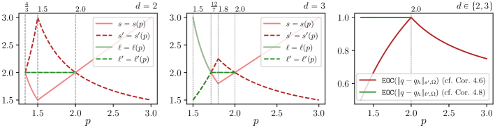
Figure 1: LEFT: Plots of $s,s^{\prime},\ell,\ell^{\prime}\in(1,\infty)$ as functions of $p\in(\frac{4}{3}(=\frac{2d}{d+1}),3)$ for $d=2$; MIDDLE: Plots of $s,s^{\prime},\ell,\ell^{\prime}\in(1,\infty)$ as functions of $p\in(\frac{9}{4}(=\frac{2d}{d+1}),3)$ for $d=3$; RIGHT: Plots of $\texttt{EOC}(\|q_{h}-q\|_{s^{\prime},\Omega})$ (cf. Corollary 12 and (82)) and $\texttt{EOC}(\|q_{h}-q\|_{\ell^{\prime},\Omega})$ (cf. Corollary 14 and (82)) as functions of $p\in(\frac{4}{3},3)$ for $d\in\{2,3\}$.

5 Numerical experiments

In this section, we review the theoretical findings of Section 4 via numerical experiments.

5.1 Implementation details

All experiments were conducted deploying the finite element software package FEniCS (version 2019.1.0), cf. [36]. In the numerical experiments, we deploy the MINI element (cf. Remark 2.7(i)) and the Taylor–Hood element (cf. Remark 2.7(ii)), each in the two-dimensional case, i.e., $d=2$:

$\bullet$ Fortin interpolation operator for the MINI element. Appealing to [4, Sec. VI.4] or [4, Appx. A.1], a Fortin interpolation operator $\Pi_{h}^{X}\colon X\to X_{h}$ for the MINI element, for every $\bm{z}\in X$, is defined by

$$\Pi_{h}^{X}\bm{z}\coloneqq\Pi_{h}^{\textit{sz},1}\bm{z}-\Pi_{h}^{\textit{corr}}(\bm{z}-\Pi_{h}^{\textit{sz},1}\bm{z})\quad\text{ in }X_{h}\,,$$

where $\Pi_{h}^{\textit{sz},1}\colon X\to\mathbb{P}^{1}(\mathcal{T}_{h})\cap X$ is the first-order Scott–Zhang quasi-interpolation operator (cf. [42]) and the local correction mapping $\Pi_{h}^{\textit{corr}}\colon X\to X_{h}$ enforcing the preservation of the discrete divergence in the $Y_{h}^{*}$-sense (cf. Assumption 6(iii)), for every $\bm{z}\in X$, is defined by

$$\Pi_{h}^{\textit{corr}}\bm{z}\coloneqq\sum_{K\in\mathcal{T}_{h}}{\smash{\frac{\langle\bm{z}-\Pi_{h}^{X}\bm{z}\rangle_{K}}{\langle b_{K}\rangle_{K}}}b_{K}}\quad\text{ in }X_{h}\,,$$

where $b_{K}\in\mathbb{P}^{3}(K)\cap W^{1,1}_{0}(K)\subseteq X_{h}$ for all $K\in\mathcal{T}_{h}$ denotes an element bubble function. Since for every $\bm{z}\in X$, by construction, it holds that $\Pi_{h}^{\textit{corr}}\bm{z}=\bm{0}$ a.e. on $\partial\Omega$ and, thus, $\Pi_{h}^{X}\bm{z}=\Pi_{h}^{\textit{sz},1}\bm{z}$ a.e. on $\partial\Omega$, it is not necessary to implement the Fortin interpolation operator $\Pi_{h}^{X}\colon X\to X_{h}$, but only the first-order Scott–Zhang quasi-interpolation operator $\Pi_{h}^{\textit{sz},1}\colon X\to\mathbb{P}^{1}(\mathcal{T}_{h})\cap X$, which is less computationally costly.

$\bullet$ Fortin interpolation operator for the Taylor–Hood element. Appealing to [18], a Fortin interpolation operator $\Pi_{h}^{X}\colon X\to X_{h}$ for the Taylor–Hood element, for every ${\bm{z}\in X}$, is defined by

$$\Pi_{h}^{X}\bm{z}\coloneqq\Pi_{h}^{\textit{sz},2}\bm{z}-\Pi_{h}^{\textit{corr}}(\bm{z}-\Pi_{h}^{\textit{sz},2}\bm{z})\quad X_{h}\,,$$

where $\Pi_{h}^{\textit{sz},2}\colon X\to\mathbb{P}^{1}(\mathcal{T}_{h})\cap X$ is the second-order Scott–Zhang quasi-interpolation opera-tor (cf. [42]) and the local correction mapping $\Pi_{h}^{\textit{corr}}\colon X\to X_{h}$ enforcing the preservation of the discrete divergence in the $Y_{h}^{*}$-sense (cf. Assumption 6(iii)), for every $\bm{z}\in X$, is defined by

$$\Pi_{h}^{\textit{corr}}\bm{z}\coloneqq\sum_{F\in\Gamma_{h}\,;\;\nu_{1},\nu_{2}\in\mathcal{N}_{h}\,\colon F=\textup{conv}\,\{\nu_{1},\nu_{2}\}}{((\operatorname{div}(\varphi^{1}_{\nu_{1}}\bm{z}),\varphi^{1}_{\nu_{2}})_{\Omega}-(\operatorname{div}(\varphi^{1}_{\nu_{2}}\bm{z}),\varphi^{1}_{\nu_{1}})_{\Omega})\,\bm{\psi}_{F}}\,,$$

where $\Gamma_{h}$ is the set of facets of $\mathcal{T}_{h}$, $\mathcal{N}_{h}$ the set of vertices of $\mathcal{T}_{h}$, $(\varphi_{\nu}^{1})_{\nu\in\mathcal{N}_{h}}\subseteq\mathbb{P}^{1}(\mathcal{T}_{h})\cap X$ nodal basis functions, and $(\bm{\psi}_{F})_{F\in\Gamma_{h}}\subseteq X_{h}$ modified tangential bubble functions (cf. [18]). Since, again, for every $\bm{z}\in X$, by construction, it holds that $\Pi_{h}^{\textit{corr}}\bm{z}=\bm{0}$ a.e. on $\partial\Omega$ and, thus, $\Pi_{h}^{X}\bm{z}=\Pi_{h}^{\textit{sz},1}\bm{z}$ a.e. on $\partial\Omega$, it is not necessary to implement the Fortin interpolation operator $\Pi_{h}^{X}\colon X\to X_{h}$, but only the second-order Scott–Zhang quasi-interpolation operator $\Pi_{h}^{\textit{sz},2}\colon X\to\mathbb{P}^{1}(\mathcal{T}_{h})\cap X$.

We approximate the discrete solution $(\bm{v}_{h},q_{h})^{\top}\in X_{h}\times Q_{h}$ of the non-linear saddle point problem (i.e., Problem (P_h)) using the Newton solver from PETSc (version 3.17.3), cf. [36], with absolute tolerance of $\tau_{abs}=1\textrm{e}{-}8$ and relative tolerance of ${\tau_{rel}=1\textrm{e}{-}10}$. The linear system emerging in each Newton iteration is solved using a sparse direct solver from MUMPS (version 5.5.0), cf. [1]. In the implementation, the uniqueness of the pressure is enforced via adding a zero mean condition.

5.2 Experimental setup

We employ Problem (Q_h) (or equivalently Problem (P_h)) to approximate the system (1)–(3) with $\bm{S}\colon\mathbb{R}^{2\times 2}\to\mathbb{R}^{2\times 2}_{\mathrm{sym}}$, where ${\Omega=(0,1)^{2}}$, for every $\bm{A}\in\mathbb{R}^{2\times 2}$ defined by

$$\bm{S}(\bm{A})\coloneqq\nu\,(\delta+|\bm{A}^{\textup{sym}}|)^{p-2}\bm{A}^{\textup{sym}}\,,$$

where $\delta\coloneqq 1\textrm{e}{-}5$, $p\in(4/3,3.0)$, $\nu\coloneqq 0.1$ if $p\geq 2$, and $\nu\coloneqq 100$ if $p<2$.

As manufactured solutions serve the vector field $\bm{v}\in X$ and the function $q\in Q^{s}$, defined by

(81) $$\bm{v}\coloneqq\tfrac{1}{10}|\cdot|^{\beta}\textrm{id}_{\mathbb{R}^{2}}\,,\qquad q\vcentcolon=|\cdot|^{\gamma}-\langle\,|\cdot|^{\gamma}\,\rangle_{\Omega}\,,$$

i.e., we choose the right-hand side $\bm{f}\in L^{p^{\prime}}(\Omega)$, the divergence $g_{1}\in L^{s}(\Omega)$ and boundary data $\bm{g}_{2}\in W^{\smash{1,1-\frac{1}{s}}}(\partial\Omega)$ accordingly.

Concerning the regularity of the velocity vector field, we choose $\beta=0.01$, which just yields that $\bm{F}(\bm{D}\bm{v})\in W^{1,2}(\Omega)$. Concerning the regularity of the pressure, we consider the two different cases covered by Corollary 12:

• We choose $\gamma=1-\smash{\frac{2}{p^{\prime}}}+0.01$, which just yields that $q\in W^{1,p^{\prime}}(\Omega)\cap L^{p^{\prime}}_{0}(\Omega)$.

• We choose $\gamma=\beta\frac{p-2}{2}+0.01$, which just yields that $(\delta+\left\lvert\bm{D}\bm{v}\right\rvert)^{\frac{2-p}{2}}|\nabla q|\in L^{2}(\Omega)$.

We construct an initial triangulation $\mathcal{T}_{h_{0}}$, where $h_{0}=1$, by subdividing the domain $\Omega=(0,1)^{2}$ along its diagonals into four triangles with different orientations. Then, finer triangulations $\mathcal{T}_{h_{i}}$, $0=1,\dots,7$, where $h_{i+1}=\frac{h_{i}}{2}$ for all $i=0,\dots,11$, are obtained by regular subdivision of the previous grid: each triangle is subdivided into four equal triangles by connecting the midpoints of the edges, i.e., applying the red-refinement rule (cf. [3, Def. 4.8(i)]).

As estimation of the convergence rates, the experimental order of convergence (EOC)

(82) $$\texttt{EOC}_{i}(e_{i})\coloneqq\frac{\log(e_{i}/e_{i-1})}{\log(h_{i}/h_{i-1})}\,,\quad i=1,\dots,7\,,$$

where for every $i=1,\dots,7$, we denote by $e_{i}$ a general error quantity.

5.3 Quasi-optimality of the error decay rates in the Corollaries 11, 12

For $p\in\{4/3,1.5,1.75,2.0,2.25,2.5,2.75,3.0\}$, the Mini and the Taylor–Hood element, in Case 1 and Case 2, and a series of triangulations $\mathcal{T}_{h_{i}}$, $i=0,\dots,7$, obtained by red-refinement as described above, we compute the corresponding discrete solutions $(\bm{v}_{h_{i}},q_{h_{i}})^{\top}\in X_{h_{i}}\times Q_{h_{i}}$, $i=0,\dots,7$, of Problem (Q_h), the error quantities

$$\left.\begin{aligned} e_{\bm{v},i}&\coloneqq\|\bm{F}(\bm{D}\bm{v}_{h_{i}})-\bm{F}(\bm{D}\bm{v})\|_{2,\Omega}\,,\\ e_{q,i}^{s}&\coloneqq\|q_{h_{i}}-q\|_{s^{\prime},\Omega}\,,\end{aligned}\quad\right\}\quad i=0,\dots,7\,,$$

and the corresponding EOCs presented in Table 1, Table 2, Table 3, and Table 4, respectively:

For both the Mini and the Taylor–Hood element as well as in Case 1 and Case 2, for the velocity errors, we report the expected convergence rate of about $\texttt{EOC}_{i}(e_{\bm{v},i})\approx\min\{1,p^{\prime}/2\}$, $i=1,\dots,7$, (in Case 1) and $\texttt{EOC}_{i}(e_{\bm{v},i})\approx 1$, $i=1,\dots,7$, (in Case 2), while for the pressure errors, only in Case 1 and if $p\in\{1.5,1.75,2.0\}$, we observe the expected convergence rate of about $\texttt{EOC}_{i}(e_{q,i}^{s})\approx p^{\prime}/2$, $i=1,\dots,7$. In both the Mini and the Taylor–Hood element as well as in Case 1 and Case 2, for the pressure errors, in the case $p>2$, we report an increased convergence rate of about $\texttt{EOC}_{i}(e_{q,i}^{s})\approx 1$, ${i=1,\dots,7}$, (in Case 1) and $\texttt{EOC}_{i}(e_{q,i}^{s})\approx 2/p^{\prime}$ , $i=1,\dots,7$, (in Case 2). Note that similar results have also been reported in [4, 32]. Putting everything together, in any case, we can confirm the quasi-optimality of the a priori error estimates for the velocity vector field derived in Corollary 11, while only in the case $p\in[1.5,2]$, we can confirm the quasi-optimality of the a priori error estimates for the pressure derived in Corollary 12.

	Case 1								Case 2
	$4/3$	1.5	1.75	2.0	2.25	2.5	2.75	3.0	2.25	2.5	2.75	3.0
$1$	0.994	0.993	0.991	0.863	0.767	0.695	0.641	0.601	0.853	0.845	0.834	0.817
$2$	0.926	0.927	0.928	0.975	0.876	0.804	0.757	0.722	0.977	0.976	0.972	0.966
$3$	0.934	0.935	0.935	0.996	0.894	0.823	0.778	0.745	1.000	1.001	1.001	0.999
$4$	0.940	0.940	0.940	1.001	0.898	0.827	0.783	0.750	1.005	1.007	1.007	1.007
$5$	0.945	0.945	0.945	1.002	0.899	0.829	0.785	0.752	1.007	1.008	1.009	1.009
$6$	0.949	0.949	0.949	1.002	0.899	0.831	0.787	0.753	1.007	1.009	1.009	1.010
$7$	0.952	0.953	0.953	1.002	0.900	0.832	0.788	0.753	1.007	1.009	1.010	1.010
theory	1.000	1.000	1.000	1.000	0.900	0.833	0.786	0.750	1.000	1.000	1.000	1.000

Table 1: Experimental order of convergence (MINI): $\texttt{EOC}_{i}(e_{\bm{v},i})$, ${i=1,\dots,7}$.

	Case 1								Case 2
	$4/3$	1.5	1.75	2.0	2.25	2.5	2.75	3.0	2.25	2.5	2.75	3.0
$1$	1.494	1.010	1.313	0.980	0.972	0.955	0.943	0.934	1.060	1.114	1.153	1.182
$2$	0.989	0.640	0.850	1.010	1.006	1.003	1.001	0.999	1.116	1.197	1.260	1.310
$3$	0.999	0.658	0.858	1.009	1.008	1.007	1.006	1.006	1.119	1.204	1.271	1.325
$4$	1.002	0.664	0.861	1.010	1.010	1.009	1.009	1.009	1.121	1.209	1.279	1.336
$5$	1.002	0.666	0.862	1.010	1.010	1.010	1.010	1.010	1.122	1.211	1.283	1.342
$6$	1.002	0.668	0.862	1.010	1.010	1.010	1.010	1.011	1.122	1.212	1.285	1.345
$7$	1.003	0.669	0.862	1.010	1.010	1.010	1.011	1.011	1.122	1.212	1.286	1.347
theory	0.500	0.667	0.875	1.000	0.900	0.833	0.786	0.750	1.000	1.000	1.000	1.000

Table 2: Experimental order of convergence (MINI): $\texttt{EOC}_{i}(e_{q,i}^{s})$, ${i=1,\dots,7}$.

	Case 1								Case 2
	$4/3$	1.5	1.75	2.0	2.25	2.5	2.75	3.0	2.25	2.5	2.75	3.0
$1$	0.990	0.991	0.994	0.793	0.733	0.683	0.644	0.614	0.789	0.782	0.769	0.744
$2$	1.007	1.008	1.007	0.982	0.880	0.812	0.766	0.730	0.981	0.978	0.974	0.966
$3$	1.009	1.010	1.010	1.005	0.897	0.828	0.783	0.748	1.004	1.003	1.002	1.000
$4$	1.008	1.010	1.010	1.009	0.900	0.832	0.786	0.752	1.009	1.008	1.008	1.008
$5$	1.008	1.009	1.010	1.010	0.901	0.833	0.788	0.753	1.010	1.010	1.009	1.009
$6$	1.007	1.009	1.010	1.010	0.901	0.834	0.789	0.754	1.010	1.010	1.010	1.010
$7$	1.007	1.008	1.010	1.010	0.901	0.835	0.789	0.755	1.010	1.010	1.010	1.010
theory	1.000	1.000	1.000	1.000	0.900	0.833	0.786	0.750	1.000	1.000	1.000	1.000

Table 3: Experimental order of convergence (Taylor–Hood): $\texttt{EOC}_{i}(e_{\bm{v},i})$, ${i=1,\dots,7}$.

	Case 1								Case 2
	$4/3$	1.5	1.75	2.0	2.25	2.5	2.75	3.0	2.25	2.5	2.75	3.0
$1$	1.255	1.011	0.987	0.965	0.967	0.967	0.968	0.970	1.057	1.121	1.170	1.211
$2$	1.256	0.961	0.990	1.005	1.004	1.002	0.999	0.997	1.111	1.191	1.255	1.308
$3$	1.171	0.890	0.985	1.009	1.008	1.008	1.007	1.006	1.119	1.204	1.272	1.327
$4$	1.101	0.822	0.981	1.010	1.010	1.009	1.009	1.009	1.121	1.209	1.280	1.337
$5$	1.051	0.770	0.974	1.010	1.010	1.010	1.010	1.010	1.122	1.211	1.283	1.343
$6$	1.023	0.739	0.967	1.010	1.010	1.010	1.010	1.010	1.122	1.212	1.285	1.345
$7$	1.008	0.720	0.958	1.010	1.010	1.010	1.010	1.010	1.122	1.212	1.286	1.347
theory	0.500	0.667	0.875	1.000	0.900	0.833	0.786	0.750	1.000	1.000	1.000	1.000

Table 4: Experimental order of convergence (Taylor–Hood): $\texttt{EOC}_{i}(e_{q,i}^{s})$, ${i=1,\dots,7}$.

5.4 Quasi-optimality of the error decay rate in Corollary 14

For $p\in\{4/3,1.4,1.45,1.5,1.75,2.0\}$, the Mini and the Taylor–Hood element, in Case 1, and a series of triangulations $\mathcal{T}_{h_{i}}$, $i=0,\dots,7$, obtained by red-refinement as described above, we compute the corresponding discrete solutions $(\bm{v}_{h_{i}},q_{h_{i}})^{\top}\in X_{h_{i}}\times Q_{h_{i}}$, $i=0,\dots,7$, of Problem (Q_h), the error quantities

$$\left.\begin{aligned} e_{q,i}^{\ell}&\coloneqq\|q_{h_{i}}-q\|_{\ell^{\prime},\Omega}\,,\\ e_{q,i}^{s}&\coloneqq\|q_{h_{i}}-q\|_{s^{\prime},\Omega}\,,\\ e_{q,i}^{p}&\coloneqq\|q_{h_{i}}-q\|_{p^{\prime},\Omega}\,,\end{aligned}\quad\right\}\quad i=0,\dots,7\,,$$

and the corresponding EOCs presented in Table 5 and Table 6, respectively:

For both the Mini and the Taylor–Hood element, for the errors $e_{q,i}^{\ell}$, $i=0,\dots,7$, we report the expected convergence rate of about $\texttt{EOC}_{i}(e_{q,i}^{\ell})\approx 1$, $i=1,\dots,7$, while for the errors $e_{q,i}^{s}$, $i=0,\dots,7$, we report a convergence rate of about ${\texttt{EOC}_{i}(e_{q,i}^{s})\approx 2/s^{\prime}}$, ${i=1,\dots,7}$ and for the errors $e_{q,i}^{p}$, $i=0,\dots,7$, we report a convergence rate of about $\texttt{EOC}_{i}(e_{q,i}^{p})\approx 2/p^{\prime}$, $i=1,\dots,7$. The increased convergence rates (compared to Corollary 12) may be explained be the fact that, for this example, we have that $q\in L^{\infty}(\Omega)$, so that from Corollary 14 together with local inverse estimates (cf. [19, Lem. 12.1]) and the $L^{\infty}$-stability of $\Pi_{h}^{Y}$ (cf. [4, Lem. 5.2]) and a standard argument, we can deduce that $\sup_{h\in(0,1]}{\|q_{h}\|_{\infty,\Omega}}<\infty$ and, thus, with real interpolation and, again, Corollary 14 that

$$\|q_{h}-q\|_{s^{\prime},\Omega}\leq\|q_{h}-q\|_{2,\Omega}^{2/s^{\prime}}\|q_{h}-q\|_{\infty,\Omega}^{1-2/s^{\prime}}\leq c\,h^{2/s^{\prime}}\,,$$

$$\|q_{h}-q\|_{p^{\prime},\Omega}\leq\|q_{h}-q\|_{2,\Omega}^{2/p^{\prime}}\|q_{h}-q\|_{\infty,\Omega}^{1-2/p^{\prime}}\leq c\,h^{2/p^{\prime}}\,.$$

Putting everything together, in any case, we can confirm the quasi-optimality of the a priori error estimates for the pressure derived in Corollary 14.

	$e_{q,i}^{\ell}$$X^{X^{X}}_{X_{X_{X}}}$						$e_{q,i}^{s}$			$e_{q,i}^{p}$
	$4/3$	1.40	1.45	1.5	1.75	2.0	$4/3$	1.40	1.45	$4/3$	1.40	1.45
$1$	1.494	1.497	1.499	1.502	1.513	1.513	1.494	1.293	1.147	0.756	0.861	0.937
$2$	0.989	0.991	0.992	0.993	1.002	1.009	0.989	0.839	0.736	0.466	0.540	0.591
$3$	0.999	1.000	1.001	1.001	1.006	1.012	0.999	0.852	0.751	0.488	0.560	0.611
$4$	1.002	1.002	1.002	1.003	1.006	1.011	1.002	0.856	0.757	0.496	0.567	0.617
$5$	1.002	1.002	1.003	1.003	1.006	1.011	1.002	0.858	0.759	0.499	0.570	0.620
$6$	1.002	1.003	1.003	1.003	1.006	1.010	1.002	0.859	0.760	0.500	0.572	0.621
$7$	1.003	1.003	1.003	1.004	1.006	1.010	1.003	0.860	0.761	0.501	0.573	0.622
theory	1.000	1.000	1.000	1.000	1.000	1.000	0.500	0.571	0.621	—	—	—

Table 5: Experimental order of convergence (MINI): $\texttt{EOC}_{i}(e_{q,i}^{\textup{a}})$, ${i=1,\dots,7}$, ${\textup{a}\in\{\ell,s,p\}}$.

	$e_{q,i}^{\ell}$$X^{X^{X}}_{X_{X_{X}}}$						$e_{q,i}^{s}$			$e_{q,i}^{p}$
	$4/3$	1.40	1.45	1.5	1.75	2.0	$4/3$	1.40	1.45	$4/3$	1.40	1.45
$1$	1.255	1.241	1.226	1.207	1.096	1.100	1.255	1.184	1.108	1.000	1.023	1.019
$2$	1.256	1.262	1.256	1.243	1.121	0.962	1.256	1.128	1.040	0.686	0.849	0.923
$3$	1.171	1.199	1.210	1.210	1.118	0.988	1.171	1.039	0.957	0.594	0.718	0.816
$4$	1.101	1.138	1.160	1.173	1.116	1.001	1.101	0.972	0.889	0.561	0.662	0.741
$5$	1.051	1.084	1.110	1.131	1.111	1.007	1.051	0.927	0.844	0.529	0.633	0.700
$6$	1.023	1.046	1.069	1.092	1.105	1.009	1.023	0.894	0.816	0.505	0.607	0.677
$7$	1.008	1.023	1.040	1.060	1.097	1.010	1.008	0.874	0.792	0.492	0.586	0.656
theory	1.000	1.000	1.000	1.000	1.000	1.000	0.500	0.571	0.621	—	—	—

Table 6: Experimental order of convergence (Taylor–Hood): $\texttt{EOC}_{i}(e_{q,i}^{\textup{a}})$, ${i=1,\dots,7}$, ${\textup{a}\in\{\ell,s,p\}}$.

6 Conclusion

For the steady, generalized Navier-Stokes system with inhomogeneous Dirichlet boundary data and an inhomogeneous divergence constraint (1)–(3), we proposed a FE discretization. We established the well-posedness, stability and (weak) convergence to a solution of the continuous problem under conditions that are similar to the existence theory for the continuous problem with inhomogeneous boundary conditions.

Then, we derived a priori error estimates for this discretization, for the velocity vector field and the kinematic pressure. The findings match the state of the art for the generalized Stokes system (cf. [4]) and for an LDG discretization (cf. [31, 32]). A new approach was followed via considering the $L^{\smash{\ell^{\prime}}}(\Omega)$-norm, where $\ell\coloneqq\max\{2,s\}$, if $p<2$. It allows for a linear error decay rate in contrast to previous results in the $L^{s^{\prime}}(\Omega)$-norm.

Numerical experiments with critical regularity have been conducted as benchmark tests complementing the theoretical findings in Section 4. These experiments confirm the quasi-optimality of the obtained a priori error estimates for the velocity vector field. The same holds for the a priori error estimates for the pressure in the $L^{p^{\prime}}(\Omega)$-norm if $p\in[{\tfrac{3d}{d+2}},2]$. If $p<2$, the linear error decay rates for the pressure error in the weaker $L^{\smash{\ell^{\prime}}}(\Omega)$-norm seem to be quasi-optimal at least if $\ell=2$, this is if $p\geq\smash{\tfrac{4d}{d+4}}$. Unfortunately, the case $p\in(\smash{\tfrac{2d}{d+1}},\smash{\tfrac{4d}{d+4}})$ could not be investigated in our setup since this interval is empty if $d=2$. Conducting respective studies for $d=3$ will be part of future research. Nevertheless, the results hint that the $L^{\smash{\ell^{\prime}}}(\Omega)$-norm is a suitable error measure for the pressure if $p<2$. The sub-optimality of the results for the pressure if $p>2$ is similar to comparable studies for the generalized Stokes system [4] and an LDG discretization [32].

Appendix A Discrete Lipschitz truncation

For the convenience of the reader, we recall a result on the discrete Lipschitz truncation and its divergence-corrected version which is used in the convergence proof. The statements are due to [14]; see also [45, Lem. 2.29, 2.30]. Due to the approximability property [17, Thm. 4.6] and density of smooth functions, our assumptions on the projection operators are sufficient.

Theorem A.1 (Discrete Lipschitz truncation).

Let Assumptions 3, 6, 5 and 4 be satisfied, let $p\in(1,\infty)$, and let $n\in\mathbb{N}$ indicate a sequence of triangulations with mesh width $h_{n}\to 0$. Assume that the sequence $\bm{v}^{n}\in V_{h_{n}}$ converges weakly to zero in $W_{0}^{1,p}(\Omega)$ as $n\to\infty$. Then, for every $n,j\in\mathbb{N}$, there exist

• real numbers $\lambda_{n,j}\in[2^{2^{j}},2^{2^{j+1}-1}]$;

• sets $B_{n,j}=\operatorname{int}(\{K\in\mathcal{T}_{h_{n},j}\})\subseteq\Omega$, where $\mathcal{T}_{h_{n},j}\subseteq\mathcal{T}_{h_{n}}$ is a subset of elements;

• truncated functions $\bm{v}^{n,j}\in W_{0}^{1,\infty}(\Omega)\cap V_{h_{n}}$;

with the following properties:

• $\bm{v}^{n,j}=\bm{v}^{n}$ on $\Omega\setminus B_{n,j}$ for all $n,j\in\mathbb{N}$;

• $\|\lambda_{n,j}\chi_{B_{n,j}}\|_{p}\leq c\,2^{-j/p}$ for all $n,j\in\mathbb{N}$;

• $\|\nabla\bm{v}^{n,j}\|_{\infty}\leq c\,\lambda_{n,j}$ for all $n,j\in\mathbb{N}$;

• $\bm{v}^{n,j}\to\bm{0}$ in $L^{\infty}(\Omega)$ $(n\to\infty)$ for all $j\in\mathbb{N}$;

• $\nabla\bm{v}^{n,j}\overset{*}{\rightharpoonup}\bm{0}$ in $L^{\infty}(\Omega)$ $(n\to\infty)$ for all $j\in\mathbb{N}$.

Lemma A.2 (Discrete divergence-corrected Lipschitz truncation).

Let the assumptions of Theorem A.1 be satisfied and suppose, in addition, that $\bm{v}^{n}\in V_{h_{n},0}$ for all $n\in\mathbb{N}$. Let $\widetilde{\bm{v}^{n,j}}\in V_{h_{n}}$ be the discrete Lipschitz truncations from Theorem A.1. Then, there is a double sequence $\bm{v}^{n,j}\in V_{h_{n},0}$, s.t.

• $\|\bm{v}^{n-j}-\widetilde{\bm{v}^{n,j}}\|_{1,p}\leq c\,2^{-j/p}$ for all $n,j\in\mathbb{N}$;

• $\bm{v}^{n,j}\to\bm{0}$ in $L^{s}(\Omega)$ $(n\to\infty)$ for all $j\in\mathbb{N}$;

• $\bm{v}^{n,j}\rightharpoonup\bm{0}$ in $W_{0}^{1,s}(\Omega)$ $(n\to\infty)$ for all $j\in\mathbb{N}$ and $s\in(1,\infty)$.

References

- [1] P. R. Amestoy, I. S. Duff, J. Koster, and J.-Y. L’Excellent, A fully asynchronous multifrontal solver using distributed dynamic scheduling, SIAM Journal on Matrix Analysis and Applications, 23 (2001), pp. 15–41.
- [2] D. N. Arnold, F. Brezzi, and M. Fortin, A stable finite element for the Stokes equations, Calcolo, 21 (1984), pp. 337–344 (1985), https://doi.org/10.1007/BF02576171.
- [3] S. Bartels, Numerical approximation of partial differential equations, vol. 64 of Texts in Applied Mathematics, Springer, 2016, https://doi.org/10.1007/978-3-319-32354-1.
- [4] L. Belenki, L. Berselli, L. Diening, and M. Růžička, On the finite element approximation of p -stokes systems, SIAM Journal on Numerical Analysis, 50 (2012), pp. 373–397, https://doi.org/10.2307/41582741.
- [5] C. Bernardi and G. Raugel, Analysis of some finite elements for the Stokes problem, Math. Comp., 44 (1985), pp. 71–79, https://doi.org/10.2307/2007793.
- [6] L. Berselli, L. Diening, and M. Ruzicka, Existence of strong solutions for incompressible fluids with shear dependent viscosities, Journal of Mathematical Fluid Mechanics, 12 (2010), pp. 101–132, https://doi.org/10.1007/s00021-008-0277-y.
- [7] E. Blavier and A. Mikelić, On the stationary quasi-newtonian flow obeying a power-law, M2AS, 18 (1995), pp. 927–948.
- [8] D. Boffi, F. Brezzi, and M. Fortin, Mixed finite element methods and applications, vol. 44 of Springer Series in Computational Mathematics, Springer, Heidelberg, 2013, https://doi.org/10.1007/978-3-642-36519-5.
- [9] S. Brenner and L. Scott, The mathematical theory of finite element methods, vol. 15 of Texts in Applied Mathematics, Springer, New York, third ed., 2008, https://doi.org/10.1007/978-0-387-75934-0.
- [10] M. Crouzeix and P.-A. Raviart, Conforming and nonconforming finite element methods for solving the stationary Stokes equations. I, Rev. Française Automat. Informat. Recherche Opérationnelle Sér. Rouge, 7 (1973), pp. 33–75.
- [11] L. Diening and F. Ettwein, Fractional estimates for non-differentiable elliptic systems with general growth, Preprint, Mathematische Fakultät, Albert-Ludwigs-Universität Freiburg, (2008), https://doi.org/10.1515/FORUM.2008.027.
- [12] L. Diening and C. Kreuzer, Linear convergence of an adaptive finite element method for the p-laplacian equation, SIAM J. Numerical Analysis, 46 (2008), pp. 614–638, https://doi.org/10.1137/070681508.
- [13] L. Diening, C. Kreuzer, and S. Schwarzacher, Convex hull property and maximum principle for finite element minimisers of general convex functionals, Numer. Math., 124 (2013), pp. 685–700, https://doi.org/10.1007/s00211-013-0527-7.
- [14] L. Diening, C. Kreuzer, and E. Süli, Finite element approximation of steady flows of incompressible fluids with implicit power-law-like rheology, SIAM Journal on Numerical Analysis, 51 (2012), https://doi.org/10.1137/120873133.
- [15] L. Diening, D. Kröner, M. Růžička, and I. Toulopoulos, A local discontinuous Galerkin approximation for systems with p-structure, IMA Journal of Numerical Analysis, 34 (2013), pp. 1447–1488, https://doi.org/10.1093/imanum/drt040.
- [16] L. Diening, J. Málek, and M. Steinhauer, On Lipschitz truncations of Sobolev functions (with variable exponent) and their selected applications, ESAIM: Control, Opt. Calc. Var., 14 (2008), pp. 211–232.
- [17] L. Diening and M. Růžička, Interpolation operators in Orlicz-Sobolev spaces, Numer. Math., 107 (2007), pp. 107–129, https://doi.org/10.1007/s00211-007-0079-9.
- [18] L. Diening, J. Storn, and T. Tscherpel, Fortin operator for the taylor–hood element, Numerische Mathematik, 150 (2022), pp. 671–689, https://doi.org/10.1007/s00211-021-01260-1.
- [19] A. Ern and J. L. Guermond, Finite Elements I: Approximation and Interpolation, no. 1 in Texts in Applied Mathematics, Springer International Publishing, 2021, https://doi.org/10.1007/978-3-030-56341-7.
- [20] P. Farrell, P. A. Gazca Orozco, and E. Süli, Finite element approximation and preconditioning for anisothermal flow of implicitly-constituted non-Newtonian fluids, Math. Comp., 91 (2022), pp. 659–697, https://doi.org/10.1090/mcom/3703.
- [21] J. Frehse, J. Málek, and M. Steinhauer, On analysis of steady flows of fluids with shear-dependent viscosity based on the Lipschitz truncation method, SIAM J. Math. Anal., 34 (2003), pp. 1064–1083.
- [22] G. P. Galdi, An introduction to the mathematical theory of the Navier-Stokes equations. Steady-state problems, Springer Monographs in Mathematics, Springer, New York, 2011, https://doi.org/10.1007/978-0-387-09620-9.
- [23] V. Girault and J.-L. Lions, Two-grid finite-element schemes for the transient Navier-Stokes problem, M2AN Math. Model. Numer. Anal., 35 (2001), pp. 945–980, https://doi.org/10.1051/m2an:2001145.
- [24] V. Girault and P.-A. Raviart, Finite element methods for Navier-Stokes equations, vol. 5 of Springer Series in Computational Mathematics, Springer-Verlag, Berlin, 1986, https://doi.org/10.1007/978-3-642-61623-5. Theory and algorithms.
- [25] V. Girault and L. R. Scott, A quasi-local interpolation operator preserving the discrete divergence, Calcolo, 40 (2003), pp. 1–19, https://doi.org/10.1007/s100920300000.
- [26] A. Hirn, M. Lanzendörfer, and J. Stebel, Finite element approximation of flow of fluids with shear rate and pressure dependent viscosity, IMA Journal of Numerical Analysis, 32 (2012), pp. 1604–1634, https://doi.org/10.1093/imanum/drr033.
- [27] E. Hopf, Ein allgemeiner Endlichkeitssatz der Hydrodynamik, Math. Ann., 117 (1941), pp. 764–775, https://doi.org/10.1007/BF01450040.
- [28] J. Jeßberger and M. Růžička, Weak solutions for steady, fully inhomogeneous generalized navier-stokes equations, 2023, https://arxiv.org/abs/2306.07094.
- [29] J. Jeßberger and M. Růžička, Existence of weak solutions for inhomogeneous generalized navier–stokes equations, Nonlinear Analysis, 212 (2021), p. 112538, https://doi.org/https://doi.org/10.1016/j.na.2021.112538.
- [30] A. Kaltenbach and M. Ruzicka, A local discontinuous galerkin approximation for the p-navier–stokes system, part i: Convergence analysis, SIAM Journal on Numerical Analysis, 61 (2023), pp. 1613–1640, https://doi.org/10.1137/22M151474X.
- [31] A. Kaltenbach and M. Ruzicka, A local discontinuous galerkin approximation for the p-navier–stokes system, part ii: Convergence rates for the velocity, SIAM Journal on Numerical Analysis, 61 (2023), pp. 1641–1663, https://doi.org/10.1137/22M1514751.
- [32] A. Kaltenbach and M. Ruzicka, A local discontinuous galerkin approximation for the p-navier–stokes system, part iii: Convergence rates for the pressure, SIAM Journal on Numerical Analysis, 61 (2023), pp. 1763–1782, https://doi.org/10.1137/22M1541472.
- [33] M. V. Korobkov, K. Pileckas, and R. Russo, Solution of Leray’s problem for stationary Navier-Stokes equations in plane and axially symmetric spatial domains, Ann. of Math. (2), 181 (2015), pp. 769–807, https://doi.org/10.4007/annals.2015.181.2.7.
- [34] J. Leray, Étude de diverses équations intégrales non linéaires et de quelques problèmes que pose l’hydrodynamique., Journal de Mathématiques Pures et Appliquées, 12 (1933), pp. 1–82, http://eudml.org/doc/235182.
- [35] J. Lions, Quelques Méthodes de Résolution des Problèmes aux Limites Non Linéaires, Dunod, Paris, 1969.
- [36] A. Logg and G. N. Wells, Dolfin: Automated finite element computing, ACM Transactions on Mathematical Software, 37 (2010), pp. 1–28, https://doi.org/10.1145/1731022.1731030.
- [37] E. Molitor and M. Růžička, On inhomogeneous –Navier–Stokes systems, in Recent Advances in PDEs and Applications, V. Radulescu, A. Sequeira, and V. Solonnikov, eds., vol. 666 of Contemp. Math., AMS Proceedings, 2016, pp. 317–340.
- [38] J. Naumann and J. Wolf, Interior differentiability of weak solutions to the equations of stationary motion of a class of non-Newtonian fluids, J. Math. Fluid Mech., 7 (2005), pp. 298–313, https://doi.org/10.1007/s00021-004-0120-z.
- [39] L. Pick, A. Kufner, O. John, and S. Fučík, Function spaces. Vol. 1, vol. 14 of De Gruyter Series in Nonlinear Analysis and Applications, Walter de Gruyter & Co., Berlin, extended ed., 2013.
- [40] M. Růžička, Nichtlineare Funktionalanalysis, Springer Verlag, Berlin, Heidelberg, 2004.
- [41] M. Ruzicka and L. Diening, Non-newtonian fluids and function spaces, 8 (2007).
- [42] L. R. Scott and S. Zhang, Finite element interpolation of nonsmooth functions satisfying boundary conditions, Math. Comp., 54 (1990), pp. 483–493,https://doi.org/10.2307/2008497.
- [43] C. Taylor and P. Hood, A numerical solution of the Navier-Stokes equations using the finite element technique, Internat. J. Comput. & Fluids, 1 (1973), pp. 73–100, https://doi.org/10.1016/0045-7930(73)90027-3.
- [44] R. Temam, Navier-Stokes equations, vol. 2 of Studies in Mathematics and its Applications, North-Holland Publishing Co., Amsterdam, third ed., 1984. Theory and numerical analysis, With an appendix by F. Thomasset.
- [45] T. Tscherpel, Finite element approximation for the unsteady flow of implicitly constituted incompressible fluids, PhD thesis, 2018, https://ora.ox.ac.uk/objects/uuid:01b4901c-9705-4087-80c1-4d656d160aed. PhD Thesis, University of Oxford.
- [46] E. Zeidler, Nonlinear functional analysis and its applications. II/B, Springer-Verlag, New York, 1990, https://doi.org/10.1007/978-1-4612-0985-0. Nonlinear monotone operators.