An energy-based model approach to rare event probability estimation

Abstract

The estimation of rare event probabilities plays a pivotal role in diverse fields. Our aim is to determine the probability of a hazard or system failure occurring when a quantity of interest exceeds a critical value. In our approach, the distribution of the quantity of interest is represented by an energy density, characterized by a free energy function. To efficiently estimate the free energy, a bias potential is introduced. Using concepts from energy-based models (EBM), this bias potential is optimized such that the corresponding probability density function approximates a pre-defined distribution targeting the failure region of interest. Given the optimal bias potential, the free energy function and the rare event probability of interest can be determined. The approach is applicable not just in traditional rare event settings where the variable upon which the quantity of interest relies has a known distribution, but also in inversion settings where the variable follows a posterior distribution. By combining the EBM approach with a Stein discrepancy-based stopping criterion, we aim for a balanced accuracy-efficiency trade-off. Furthermore, we explore both parametric and non-parametric approaches for the bias potential, with the latter eliminating the need for choosing a particular parameterization, but depending strongly on the accuracy of the kernel density estimate used in the optimization process. Through three illustrative test cases encompassing both traditional and inversion settings, we show that the proposed EBM approach, when properly configured, (i) allows stable and efficient estimation of rare event probabilities and (ii) compares favorably against subset sampling approaches.

1 Introduction

Estimating rare event probabilities is a fundamental challenge in various fields, including finance, engineering and environmental sciences. Rare events are characterized by their low occurrence rates, but they become crucial when their outcomes have substantial consequences (Juneja and Shahabuddin, 2006). In the field of uncertainty quantification, rare events are frequently related to the failure of engineering systems that are designed to be highly reliable (Beck and Zuev, 2015), examples of which include hydroelectric dams, airplanes, or nuclear reactors. In these cases, the accurate estimation of rare event probabilities is of utmost importance as it enables informed decision-making, effective risk management, and the design of robust systems.

In practical applications, there are commonly no analytical formulas for estimating rare event probabilities. To address this issue, asymptotic approximation methods such as the first-order reliability method (FORM; Hasofer and Lind 1974) have been proposed. However, relying solely on FORM results without understanding the characteristics of the linearized domains, particularly in higher dimensions, is not recommended (Straub et al., 2016). On the other hand, conventional Monte Carlo simulation methods are often computationally inefficient. Consequently, a considerable amount of research has been dedicated to developing more efficient stochastic simulation techniques for rare event probability estimations (e.g., Bucklew 2004, Rubino and Tuffin 2009). Beck and Zuev (2015) present two principal stochastic simulation approaches: importance sampling and subset simulation. Importance sampling is a variance reduction technique, aiming to increase sampling frequency in the region of interest, which in the present context corresponds to the region containing the rare event and its vicinity (e.g., Au and Beck 1999). Subset simulation (Au and Beck, 2001) represents a rare event probability as a product of larger probabilities, effectively breaking down the rare event into less rare conditional events (e.g., Au and Wang 2014). While subset sampling explores a wide range of parameter combinations, the more directed line sampling (e.g., Hohenbichler and Rackwitz 1988, Koutsourelakis et al. 2004) generates samples on a hyperplane that is orthogonal to a significant direction pointing to the rare event region.

In this study, we are particularly interested in rare event probability estimation in the context of an underlying inverse problem. We employ non-linear Bayesian inversion aiming to infer unknown properties $\boldsymbol{\theta}$ given measurements $\boldsymbol{y}$. Instead of being interested in the posterior distribution itself, we target the distribution of a real-valued quantity of interest that depends on the unknown properties through a non-linear relationship $\boldsymbol{\theta}\mapsto\mathcal{R}(\boldsymbol{\theta})$. More particularly, we would like to estimate the probability of this quantity exceeding a critical threshold, $\mathbb{P}(\mathcal{R}(\boldsymbol{\theta})\geq T|\boldsymbol{y})$, which is related to the problem of evaluating the probability of failure of a system. As the underlying relationships are non-linear, analytical formulas for the distribution of $\mathcal{R}(\boldsymbol{\theta})$ conditioned on the data $\boldsymbol{y}$ are typically not available. In structural reliability engineering, similar problems have been targeted with data first being used to update $\boldsymbol{\theta}$ and then apply these updated distributions to the prediction of rare events (e.g., Papadimitriou et al. 2001, Jensen et al. 2013, Sundar and Manohar 2013, Hadjidoukas et al. 2015). Specialized estimation methods are essential since conventional Monte Carlo approaches relying on posterior samples would typically demand overwhelmingly large sample sizes.

In practice, most structural reliability methods encounter difficulties when starting with a sample approximation of the posterior, but subset sampling is an exception (Straub et al., 2016). In an inversion context, it was employed to estimate the so-called “updated robust failure probability” by Jensen et al. (2013) and Hadjidoukas et al. (2015). Also in the engineering literature, Straub (2011) introduced Bayesian Updating with Structural reliability methods for posterior inference (BUS; e.g. Straub and Papaioannou 2015). This method can be considered as an extension of rejection sampling that aims to overcome its inefficiency by treating the acceptance event as a rare event using structural reliability methods (e.g., FORM, subset simulation and line sampling; see Straub et al. 2016). It offers a framework, in which the rare event probability under the posterior can be estimated directly within the framework of structural reliability analysis. A recent advancement to the BUS framework involves the utilization of cross entropy-based importance sampling, which enables efficient sampling from the critical region of the posterior failure domain (Kanjilal et al., 2023).

Free energy is a fundamental concept in materials science and physical chemistry (Stecher et al., 2014). Performing the free energy estimation on crude Monte Carlo draws is rarely practical as it would need an excessively large number of samples to sufficiently cover the whole range of the states, particularly in a rare event setting as ours. To address this challenge, one solution is to enhance the sampling in specific regions of interest by introducing a bias term. This approach, known as umbrella or non-Boltzmann sampling, can be traced back to the work of Torrie and Valleau (1977), who demonstrated how to recover the unbiased probability distribution from the biased samples. Applications for free energy functions are numerous (e.g., Stecher et al. 2014, Kästner and Thiel 2005). More recently, Shirts and Ferguson (2020) introduced a Bayesian formalism to estimate the free energy function by minimizing the Kullback–Leibler divergence between a continuous trial function and the empirical samples generated by biased sampling. Constructing a bias potential is a non-trivial task, therefore, Valsson and Parrinello (2014) introduced a variational approach that adaptively combines exploration and reconstruction by iteratively improving and refining the bias potential and the free energy function. The approach by Valsson and Parrinello (2014) not only utilizes the bias potential to improve the sampling technique employed for optimizing the free energy function (as with umbrella sampling), but also depends on it to directly estimate the free energy function. This variationally-enhanced sampling method has been applied in the context of coarse-graining methods by Invernizzi et al. (2017) and combined with machine-learning techniques by Bonati et al. (2019).

By employing concepts from energy-based models (EBMs), we propose a new formulation and approach to solve rare event probability estimation problems. We write the marginal posterior distribution of the quantity of interest $R=\mathcal{R}(\boldsymbol{\theta})$ as an energy density function with free energy $r\mapsto F(r)$. To estimate $F(r)$ efficiently in the region of interest, a bias potential $r\mapsto V(r)$ and a corresponding probability density function (PDF) $r\mapsto p_{V}(r)\propto\exp(-(F(r)+V(r)))$, are introduced. That is, the energy density function of $R$ (knowing $\boldsymbol{y}$) is $p_{0}(r)$, where 0 refers to a zero-valued bias potential. The considered EBM (Goodfellow et al. 2016) approach relies on optimizing the bias potential $V(r)$ such that $p_{V}(r)$ approximates a pre-defined PDF $p_{\textup{ref}}(r)$, which is selected such that it has high probability mass in the targeted region. Given the optimal bias potential $V(r)$, it is straightforward to derive the free energy $F(r)$ with an accurate estimation in the region where $p_{\textup{ref}}(r)$ has most of its mass being emphasized. Our approach is related to the variational method by Valsson and Parrinello (2014), but we adopt the fundamental concepts of their method within a different formulation and apply it to a novel context, that is, rare event probability estimation. Practically, in EBM methods, the potential $V(r)$ is parameterized using methods such as neural networks, splines or radial basis functions. In Valsson and Parrinello (2014), the optimal $V(r)$ is approximated by minimizing a loss function which is related to the Kullback–Leibler divergence between $p_{\textup{ref}}(r)$ and $p_{V}(r)$ using stochastic optimization methods. We adapt this approach and add a stopping criterion based on the Stein discrepancy (Gorham and Mackey, 2015) to achieve a balance between computational efficiency and satisfactory model performance. Furthermore, we introduce a non-parametric approach for the bias potential, thereby alleviating the challenge of selecting an appropriate parameterization.

The proposed EBM approach reduces the potentially high-dimensional problem of estimating the posterior distribution of $\boldsymbol{\theta}$ and subsequently $\mathcal{R}(\boldsymbol{\theta})$ to an optimization of a one-dimensional function $V:\mathbb{R}\rightarrow\mathbb{R}$. Importantly, the EBM approach is not limited to inversion settings and can also be effectively applied to traditional rare event probability estimation. We examine the performance of our proposed method using three illustrative test examples. The first example targets the probability of high contamination values endangering organism living in the soil. The presence of an analytical solution allows us to explore the EBM method’s sensitivity to implementation variables. Next, we consider the two-dimensional four-branch function problem, commonly used as a benchmark in reliability analysis. This example does not involve inversion and demonstrates the method’s suitability for general rare event estimation scenarios. Last, we use a simple load and capacity example from Straub et al. (2016) to compare the EBM method’s performance against their BUS approach. The manuscript is organized as follows: Section 2 introduces the problem setting, outlines our energy-based model approach, and details the methods employed for comparison. In Section 3, the test examples are presented. Subsequently, Section 4 discusses the results, leading to the conclusions exposed in Section 5.

2 Methodology

2.1 Problem setting

In the considered rare event setting, we target a quantity of interest $R=\mathcal{R}(\boldsymbol{\theta})$ derived from the random vector $\boldsymbol{\theta}$ on $\mathbb{R}^{d}$ by some non-linear function $\mathcal{R}:\mathbb{R}^{d}\rightarrow\mathbb{R}$. We consider a rare set $A=\{\boldsymbol{\theta}\in\mathbb{R}^{d}:\mathcal{R}(\boldsymbol{\theta})\geq T\}$ with $T\in\mathbb{R}$ and want to estimate $\mathbb{P}(\boldsymbol{\theta}\in A)$. In a traditional rare event setting, we consider $\boldsymbol{\theta}$ distributed according to a prior PDF $p_{\boldsymbol{\theta}}(\boldsymbol{\theta})$, which is absolutely continuous with respect to a dominating measure, typically the Lebesgue measure on $\mathbb{R}^{d}$. The rare event probability can then be expressed as,

$$\mathbb{P}(\mathcal{R}(\boldsymbol{\theta})\geq T)=\mathbb{P}(\boldsymbol{\theta}\in A)=\int_{A}p_{\boldsymbol{\theta}}(\boldsymbol{\theta})\mathrm{d}\boldsymbol{\theta}.$$ (1)

Bayesian probabilistic inversion methods target generally unknown properties $\boldsymbol{\theta}$ and seek to infer their posterior PDF given the measurements $\boldsymbol{y}\in\mathbb{R}^{m}$. In most applications, the random data vector is given by $\boldsymbol{Y}=\mathcal{G}(\boldsymbol{\theta})+\boldsymbol{\varepsilon_{\mathcal{O}}}$, with $\mathcal{G}:\mathbb{R}^{d}\rightarrow\mathbb{R}^{m}$ referring to the forward operator and $\boldsymbol{\varepsilon_{\mathcal{O}}}$ to the observational noise. In Bayes’ theorem, the posterior PDF of the target parameters $\boldsymbol{\theta}$ given measurements $\boldsymbol{y}$ is given by,

$$p_{\boldsymbol{\theta}|\boldsymbol{Y}}(\boldsymbol{\theta}|\boldsymbol{y})=\frac{p_{\boldsymbol{\theta}}(\boldsymbol{\theta})p_{\boldsymbol{Y}|\boldsymbol{\theta}}(\boldsymbol{y}|\boldsymbol{\theta})}{p_{\boldsymbol{Y}}(\boldsymbol{y})},$$ (2)

with the prior PDF $p_{\boldsymbol{\theta}}(\boldsymbol{\theta})$, the likelihood function $p_{\boldsymbol{Y}|\boldsymbol{\theta}}(\boldsymbol{y}|\boldsymbol{\theta})$ and the evidence $p_{\boldsymbol{Y}}(\boldsymbol{y})$ (assumed non-zero). Assuming independent Gaussian observational errors, the likelihood is expressed as $p_{\boldsymbol{Y}|\boldsymbol{\theta}}(\boldsymbol{y}|\boldsymbol{\theta})=\varphi_{m}(\boldsymbol{y};\mathcal{G}(\boldsymbol{\theta}),\boldsymbol{\Sigma_{\boldsymbol{Y}}})$, with $\varphi_{m}(\cdot;\boldsymbol{\mu},\boldsymbol{\Sigma})$ denoting the PDF of a $m$-variate normal distribution with mean $\boldsymbol{\mu}$ and diagonal covariance matrix $\boldsymbol{\Sigma}$ with the variance of the observational error on its diagonal. For $\boldsymbol{\theta}$ distributed according to a Bayesian posterior PDF $\boldsymbol{\theta}\mapsto p_{\boldsymbol{\theta}|\boldsymbol{Y}}(\boldsymbol{\theta}|\boldsymbol{y})$, we aim to estimate,

$$\mathbb{P}(\mathcal{R}(\boldsymbol{\theta})\geq T|\boldsymbol{y})=\mathbb{P}(\boldsymbol{\theta}\in A|\boldsymbol{y})=\int_{A}p_{\boldsymbol{\theta}|\boldsymbol{Y}}(\boldsymbol{\theta}|\boldsymbol{y})\mathrm{d}\boldsymbol{\theta}.$$ (3)

2.2 Energy-based model approach

While our methodology is formulated for an inversion setting, it can be readily adjusted to suit a conventional rare event estimation scenario with $\boldsymbol{\theta}$ being distributed according to a prior PDF.

We write the posterior PDF of $\boldsymbol{\theta}$ as an energy density function,

$$p_{\boldsymbol{\theta}|\boldsymbol{Y}}(\boldsymbol{\theta}|\boldsymbol{y})=\frac{\exp(-U(\boldsymbol{\theta}))}{Z},\quad Z:=\int\exp(-U(\zeta))\mathrm{d}\zeta,$$ (4)

with free energy $U(\boldsymbol{\theta})=-\log p_{\boldsymbol{Y}|\boldsymbol{\theta}}(\boldsymbol{y}|\boldsymbol{\theta})-\log p_{\boldsymbol{\theta}}(\boldsymbol{\theta})$. The marginal posterior distribution of the quantity of interest $R=\mathcal{R}(\boldsymbol{\theta})$ is thus given by,

$$p_{R|\boldsymbol{Y}}(r|\boldsymbol{y})=\int\frac{\exp(-U(\boldsymbol{\theta}))}{Z}\delta(r-\mathcal{R}(\boldsymbol{\theta}))\mathrm{d}\boldsymbol{\theta}.$$ (5)

More details on the definition of such integrals can be found in Lelièvre et al. (2010) (Lemma 3.2; co-area formula). We write $p_{R|\boldsymbol{Y}}(r|\boldsymbol{y})$ as an energy density function with (unknown) free energy $r\mapsto F(r)$,

$$p_{R|\boldsymbol{Y}}(r|\boldsymbol{y})=\exp(-F(r)).$$ (6)

In order to estimate $F(r)$ and $p_{R|\boldsymbol{Y}}(r|\boldsymbol{y})$, we have the option of utilizing posterior samples obtained from $p_{\boldsymbol{\theta}|\boldsymbol{Y}}(\boldsymbol{\theta}|\boldsymbol{y})$ and applying a transformation $\boldsymbol{\theta}\mapsto\mathcal{R}(\boldsymbol{\theta})$. Since this follows a typical Monte Carlo approach, it would need an impractically large number of samples to include the low probability regions of $p_{R|\boldsymbol{Y}}(r|\boldsymbol{y})$ that are of interest. To enhance sampling in the region of interest, we seek to sample in accordance to a pre-defined $p_{\textup{ref}}(r)$ with most mass on the set $\{R\geq T\}$. To achieve this, we introduce the bias potential $r\mapsto V(r)$ and the PDF $r\mapsto p_{V}(r)$,

$$p_{V}(r)=\frac{\exp(-(F(r)+V(r)))}{\int\exp(-(F(s)+V(s)))\mathrm{d}s}.$$ (7)

We seek $p_{V}(r)=p_{\textup{ref}}(r)$, which holds for $V_{\textup{opt}}(r)=-F(r)-\log(p_{\textup{ref}}(r))$ (for $p_{\textup{ref}}(r)>0$, ignoring an irrelevant constant). Given $V_{\textup{opt}}(r)$, it is straightforward to obtain $F(r)$ as $F(r)=-\log(p_{\textup{ref}}(r))-V_{\textup{opt}}(r)$, for $p_{\textup{ref}}(r)>0$ and hence $p_{R|\boldsymbol{Y}}(r|\boldsymbol{y})$. Eventually, we can express the probability of the rare event as,

$$\mathbb{P}(\mathcal{R}(\boldsymbol{\theta})\geq T|\boldsymbol{y})=\int_{T}^{\infty}p_{R|\boldsymbol{Y}}(r|\boldsymbol{y})\mathrm{d}r=\int_{T}^{\infty}\exp(-F(r))\mathrm{d}r.$$ (8)

A basic visualization of the EBM approach is given in Figure 1.

Figure 1: Illustration of the energy-based model approach. (a) For $V(r)=0$, $p_{V}(r)=p_{R|\boldsymbol{Y}}(r|\boldsymbol{y})$ has low probability mass on the set $\{R\geq T\}$. (b) For $V(r)\approx V_{\textup{opt}}(r)$, $p_{V}(r)\approx p_{\textup{ref}}(r)$ yielding by design a high probability mass on the set $\{R\geq T\}$.

An important choice is the definition of $p_{\textup{ref}}(r)$. When the PDF of $p_{R|\boldsymbol{Y}}(r|\boldsymbol{y})$ is supported by a compact interval with length $\Omega_{p}$, one possible and natural choice is to set $p_{\textup{ref}}(r)=1/\Omega_{p}$ (Valsson and Parrinello, 2014). This results in uniform sampling and is commonly employed in other enhanced sampling approaches (Wang and Landau, 2001). If the support is unbounded, then $p_{\textup{ref}}(r)$ can be selected such that it shifts mass to the range of $R$ which is of interest (here $R\geq T$). To enable accurate rare event probability estimation, the right tails of the selected $p_{\textup{ref}}(r)$ have to be at least as heavy as the tails of the target PDF $p_{R|\boldsymbol{Y}}(r|\boldsymbol{y})$.

2.2.1 Parameterization and optimization of $V(r)$

We parameterize the bias potential $V(r)$ using a flexible model $V_{\psi}(r)$ with free parameters $\psi$. We employ here radial basis functions (RBFs) with squared exponential kernels,

$$V_{\psi}(r)=\sum_{j=1}^{B}w_{j}\phi(r-b_{j}),\text{ where }\phi(r)=\exp(-(\kappa_{j}r)^{2}).$$ (9)

For a number $B$ of RBFs, we obtain $\psi=(\mathbf{w,b,\kappa})\in\mathbb{R}^{B}\times\mathbb{R}^{B}\times\mathbb{R}^{B}$. Then, we seek the optimal $V_{\psi}(r)$ by minimizing the Kullback–Leibler divergence between $p_{\textup{ref}}(r)$ and $p_{V_{\psi}}(r)$ with respect to $\psi$. We achieve this by employing stochastic gradient descent with momentum (SGDM; e.g., Liu et al. 2020),

$$m_{n} =\beta m_{n-1}+(1-\beta)\frac{\partial\textup{KL}(p_{\textup{ref}}||p_{V_{\psi}})}{\partial\psi},$$ (10)

$$\psi_{n+1} =\psi_{n}-\gamma m_{n},$$

using initial momentum $m_{0}=0$, momentum weight $\beta$, learning rate $\gamma$ and a stochastic gradient of $\textup{KL}(p_{\textup{ref}}||p_{V_{\psi}})$ at $\psi_{n}$. For a momentum weight of $\beta=0$, SDGM reduces to traditional stochastic gradient descent.

It holds that

$$\textup{KL}(p_{\textup{ref}}||p_{V_{\psi}}) =\int p_{\textup{ref}}(r)\log p_{\textup{ref}}(r)\mathrm{d}r-\int p_{\textup{ref}}(r)\log p_{V_{\psi}}(r)\mathrm{d}r$$ (11)

$$=\textup{const.}+\int p_{\textup{ref}}(r)V_{\psi}(r)\mathrm{d}r+\log\int\exp(-(F(s)+V_{\psi}(s)))\mathrm{d}s,$$

and (assuming standard regularity assumptions that allow swapping the order of differentiation and integration),

$$\frac{\partial\textup{KL}(p_{\textup{ref}}||p_{V_{\psi}})}{\partial\psi} =\frac{\partial}{\partial\psi}\int p_{\textup{ref}}(r)V_{\psi}(r)\mathrm{d}r+\frac{\partial}{\partial\psi}\log\int\exp(-(F(s)+V_{\psi}(s)))\mathrm{d}s$$ (12)

$$=\int p_{\textup{ref}}(r)\frac{\partial}{\partial\psi}V_{\psi}(r)\mathrm{d}r-\int p_{V_{\psi}}(s)\frac{\partial}{\partial\psi}V_{\psi}(s)\mathrm{d}s.$$

This allows us to approximate,

$$\frac{\partial\textup{KL}(p_{\textup{ref}}||p_{V_{\psi}})}{\partial\psi}\approx\frac{1}{n}\sum_{i=1}^{n}\frac{\partial}{\partial\psi}V_{\psi}(r_{i})-\frac{1}{n}\sum_{i=1}^{n}\frac{\partial}{\partial\psi}V_{\psi}(s_{i}),\quad\text{ with }r_{i}\sim p_{\textup{ref}}(\cdot),s_{i}\sim p_{V_{\psi}}(\cdot).$$ (13)

This requires samples from $p_{V_{\psi}}(\cdot)$ and $p_{\textup{ref}}(\cdot)$, with the latter being straightforward as the PDF $p_{\textup{ref}}(\cdot)$ is pre-defined. Sampling from $p_{V_{\psi}}(\cdot)$ directly is not possible as it would require that $F(r)$ was known. Thus, we use samples of the original space of $\boldsymbol{\theta}$ by introducing,

$$p_{V_{\psi}}(\boldsymbol{\theta})=\frac{\exp(-(U(\boldsymbol{\theta})+V_{\psi}(\mathcal{R}(\boldsymbol{\theta}))))}{\int\exp(-(U(\boldsymbol{\zeta})+V_{\psi}(\mathcal{R}(\boldsymbol{\zeta}))))d\boldsymbol{\zeta}},$$ (14)

and then transform them using $\mathcal{R}(\cdot)$. This is correct as one can easily check that the following identity $\int p_{V_{\psi}}(\boldsymbol{\theta})\delta(r-\mathcal{R}(\boldsymbol{\theta}))d\boldsymbol{\theta}=p_{V_{\psi}}(r)$ holds. In our implementation, the samples of $p_{V_{\psi}}(\boldsymbol{\theta})$ are obtained using a Metropolis–Hastings algorithm (MH; Metropolis et al. 1953; Hastings 1970).

This idea of optimizing the bias potential to estimate the free energy coincides with the variational approach of Valsson and Parrinello (2014), Invernizzi et al. (2017) and Bonati et al. (2019) introduced in metadynamics, working with the functional,

$$\Omega(V)=\log\left(\frac{\int\exp(-(F(r)+V(r)))\mathrm{d}r}{\int\exp(-F(r))\mathrm{d}r}\right)+\int p_{\textup{ref}}(r)V(r)\mathrm{d}r,$$ (15)

which they show is convex and invariant under the addition of an arbitrary constant to $V(r)$. It is easy to show that minimizing $\Omega(V)$ is equivalent to minimizing $\textup{KL}(p_{\textup{ref}}||p_{V})$ (e.g. Invernizzi et al. 2017). Furthermore, we can reformulate the minimization of the Kullback–Leibler divergence as a maximum likelihood estimation problem (Appendix A), which offers multiple theoretical possibilities as it allows us to transfer known theoretical results on maximum likelihood estimation to our approach.

2.2.2 Non-parametric bias potential $V(r)$

In addition to the parametric bias potentials $V_{\psi}$ considered so far, the functional $\Omega(V)$ of Eq. (15) can be applied to a broader class of bias potentials $V$. While Invernizzi et al. 2017 is not really giving details regarding the source space on which $\Omega(V)$ is defined, it is noticeable that for $V$ integrable with respect to $p_{\text{ref}}$, $\Omega(V)$ can be seen as a convex functional (taking infinite values in case of non-integrable $\exp(-F-V))$. Furthermore, for suitable $V$ and directions $H$, one can work out directional derivatives of $\Omega$

$$\mathrm{d}\Omega(V;H)=\int p_{\textup{ref}}(r)H(r)\mathrm{d}r-\int p_{V}(r)H(r)\mathrm{d}r=\int(p_{\textup{ref}}(r)-p_{V}(r))H(r)\mathrm{d}r.$$ (16)

In particular, for bounded $V$ and $p_{\text{ref}}$ as considered herein, the directional derivative at $V$ in the direction $p_{\textup{ref}}-p_{V}$ is well defined and $p_{V}-p_{\textup{ref}}$ delivers a descent direction. In sequential settings, the function $V_{n}$ can be updated with SGDM (Eq. 10) using $p_{\textup{ref}}-p_{V}$ in lieu of stochastic gradient at $V_{n}$. While for the PDF $p_{\textup{ref}}$, we have access to its analytical form, we rely here in practice for $p_{V_{n}}$ on a kernel density estimate derived from the MH samples.

2.2.3 Stopping criteria

Appropriate stopping criteria are crucial when employing stochastic gradient-based optimization in order to strike a balance between computational efficiency and achieving satisfactory model performance. One naïve approach is to stop the training after a pre-defined number of optimization steps. Since this approach does not ensure convergence if the selected number is too low or might waste computational resources if chosen to be too high, it makes sense to monitor the values of the loss function and terminate the optimization when it reaches a desired criterion or when it no longer improves significantly.

Here we consider a convergence measure based on Stein’s method (Stein, 1972): the Stein discrepancy (Gorham and Mackey, 2015). To circumvent the latter’s computational intractability, we use a specific version known as the kernel Stein discrepancy (KSD; Liu et al. 2016, Chwialkowski et al. 2016, Gorham and Mackey 2017),

$$KSD(p_{\textup{ref}}||p_{V_{\psi}})= \sqrt{\frac{1}{n^{2}}\sum_{i,j=1}^{n}k_{p_{\textup{ref}}}(r_{i},r_{j})},\quad r_{i}\sim p_{V_{\psi}}(\cdot),\text{ with, }$$ (17)

$$k_{p_{\textup{ref}}}(r,s)= \nabla_{r}\nabla_{s}k(r,s)+\langle\nabla_{r}k(r,s),\nabla_{s}\log p_{\textup{ref}}(s)\rangle+\langle\nabla_{s}k(r,s),\nabla_{r}\log p_{\textup{ref}}(r)\rangle$$

$$+k(r,s)\langle\nabla_{r}\log p_{\textup{ref}}(r),\nabla_{s}\log p_{\textup{ref}}(s)\rangle,$$

with kernel $k(r,s)$. The use of the KSD is particularly advantageous in our setting due to the analytical knowledge about the probability distribution $p_{\textup{ref}}(r)$.

As stopping criterion, we employ a statistical test for goodness-of-fit based on the squared KSD (Liu et al. 2016, Chwialkowski et al. 2016). Employing bootstrap sampling for the estimation of the test statistic, the algorithm stops as soon as the null hypothesis of $p_{\textup{ref}}=p_{V_{\psi}}$ cannot be rejected with a significance level of $\alpha$ anymore. To counteract the conservative nature of the test procedure when dealing with the correlated samples resulting from MH, Chwialkowski et al. (2016) suggest an approach based on the wild bootstrap technique (e.g., Shao 2010). The proposed test statistics $S$ takes into account the correlation structure in the samples by mimicking it with an auxiliary Markov chain taking values in $\{-1,1\}$,

$$S=\frac{1}{n^{2}}\sum_{i,j=1}^{n}W_{i}W_{j}k_{p_{\textup{ref}}}(r_{i},r_{j}),\quad\text{using}\quad W_{i}=\mathbbm{1}(U_{i}>a_{BS})W_{i-1}-\mathbbm{1}(U_{i}<a_{BS})W_{i-1},$$ (18)

where $W_{1}=1$ and $U_{i}\sim\textup{Unif}(0,1)$. Chwialkowski et al. (2016) suggest combining this method with thinning of the generated samples. They recommend to thin the chain such that $\textup{Cor}(r_{i},r_{i-1})<0.5$, set $a_{BS}=0.1/q$ with $q<10$ and use at least $n=\max(500q,100)$ samples.

2.2.4 Related work in machine learning

Energy-based models are a popular class of probabilistic models in machine learning (Goodfellow et al., 2016). In this context, EBMs are used to model the distribution of available data $(r_{i})_{i=1}^{N}$ (say images) distributed according to an unknown PDF $p_{\textup{ref}}(r)$ via a model of the form

$$p_{\psi}(r)=\frac{\exp(-U_{\psi}(r))}{Z_{\psi}},$$ (19)

the potential $U_{\psi}(r)$ being typically parameterized by a neural network. The parameter $\psi$ can be learned by maximizing the normalized log-likelihood, that is,

$$\ell_{N}(\psi)=\frac{1}{N}\sum_{i=1}^{N}\log p_{\psi}(r_{i}),$$ (20)

which approximates up to an additive constant independent of $\psi$ the Kullback–Leibler divergence $\textup{KL}(p_{\textup{ref}}||p_{\psi})$ as $N\rightarrow\infty$ (Appendix A). Similarly to our scenario, the gradient of this discrepancy requires sampling from $p_{\psi}(r)$ using Markov chain Monte Carlo.

Compared to applications in machine learning, the rare event simulation context discussed in this paper enjoys several attractive properties. First, we can obtain as many samples from $p_{\textup{ref}}(r)$ as we want. Second, because we know $p_{\textup{ref}}(r)$ analytically, we can assess how good our estimate of $p_{\textup{ref}}(r)$ is via $p_{\psi}(r)$ as discussed in Section 2.2.3. Third, we only need to estimate a one-dimensional function $V_{\psi}(r)$ instead of a complex high-dimensional potential $U_{\psi}(r)$. We note finally that numerous alternatives to Kullback–Leibler minimization have been developed to train EBMs and that some of them might be applicable to the rare event simulation context, see Song and Kingma (2021) for a recent review.

2.3 Alternative rare event probability estimation methods

2.3.1 Subset sampling

Subset sampling for rare event probability estimation was introduced by Au and Beck (2001) and is based on the realization that the probability of a rare event can be expressed as a multiplication of higher conditional probabilities involving intermediate failure events. To estimate $\mathbb{P}(\boldsymbol{\theta}\in A|\boldsymbol{y})=\mathbb{P}(\mathcal{R}(\boldsymbol{\theta})\geq T|\boldsymbol{y})$, subset sampling employs a sequence of thresholds $\{T_{0},...,T_{K}\}$ with $T_{0}=-\infty$ and $T_{K}=T$ and corresponding nested sets $A_{k}=\{\boldsymbol{\theta}\in\mathbb{R}^{d}:\mathcal{R}(\boldsymbol{\theta})\geq T_{k}\}$. It holds that,

$$\mathbb{P}(\boldsymbol{\theta}\in A|\boldsymbol{y})=\prod\limits_{k=1}^{K}\mathbb{P}(\boldsymbol{\theta}\in A_{k}|\boldsymbol{\theta}\in A_{k-1},\boldsymbol{y}).$$ (21)

Au and Beck (2001) propose to select the sequence of thresholds adaptively such that a ratio of $(1-\gamma)$ of the samples survive. Such an adaptive procedure leads to positively biased estimates, however, this bias decreases with an increasing number of samples per subset (Cérou et al., 2012). To use subset sampling in our inversion setting, we initialize the first set of samples with a draw from the posterior using the states sampled by a MH algorithm after burn-in. In this context, the thinning factor is critical as the initial set of samples should be as independent as possible. We then propagate the set of samples to estimate the conditional probabilities by sampling from the subsets while accounting for the posterior. A similar approach was applied by Jensen et al. (2013), who rely on transitional MCMC to generate the first set of posterior samples.

2.3.2 Bayesian updating of rare event probabilities

In the article by Straub and Papaioannou (2015), building upon their previous work presented in Straub (2011), a methodological framework called Bayesian Updating with Structural reliability methods (BUS) is introduced. This method serves as an extension of the conventional rejection sampling technique in Bayesian analysis. In a basic version of rejection sampling, samples are generated from the prior distribution and subsequently accepted with a probability of $p_{\boldsymbol{Y}|\boldsymbol{\theta}}(\boldsymbol{y}|\boldsymbol{\theta})/\bar{p}$, where $\bar{p}$ is an upper bound on $\mathrm{sup}_{\boldsymbol{\theta}}p_{\boldsymbol{Y}|\boldsymbol{\theta}}(\boldsymbol{y}|\boldsymbol{\theta})$. The issue with the basic rejection sampling algorithm is its inefficiency, particularly when dealing with high-dimensional or complex posterior distributions. The core concept behind BUS is to address the challenge posed by the small acceptance probabilities in rejection sampling with structural reliability methods.

We consider BUS with subset sampling, employing the principles of subset sampling (Section 2.3.1) to sample from the acceptance region of the extended rejection sampling algorithm, while enabling an adaptive estimation of the constant $\bar{p}$ (Betz et al., 2014). In the study of Straub et al. (2016), this method strikes an appropriate balance between accuracy and the number of model evaluations and has the advantage of being more robust compared to line sampling that they also consider. To apply BUS for rare event probability estimation in an inversion setting, Straub et al. (2016) combine two subset sampling runs, where the first generates samples from the posterior and the second propagates these samples towards the targeted rare event. This approach is comparable to the subset sampling method described in Section 2.3.1 with the difference that the posterior sampling part is replaced with BUS.

3 Illustrative test examples

We now explore the performance of our EBM method in different illustrative test examples. We start with exploring the method’s sensitivity to the choice of configuration using a hypothetical contamination problem for which an analytical solution is available. Next, we consider the two-dimensional four-branch function problem, a frequently utilized benchmark in reliability analysis. This example does not require inversion and effectively demonstrates the method’s suitability for more traditional rare event estimation scenarios. For both of these first examples, we compare the EBM method against a standard implementation of subset sampling. Finally, we consider a simple load and capacity example of Straub et al. (2016) to compare the EBM method’s performance against the BUS approach with subset sampling.

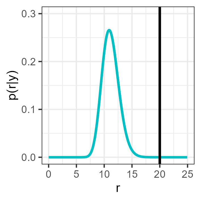
(a)

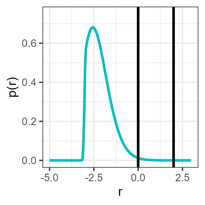
(b)

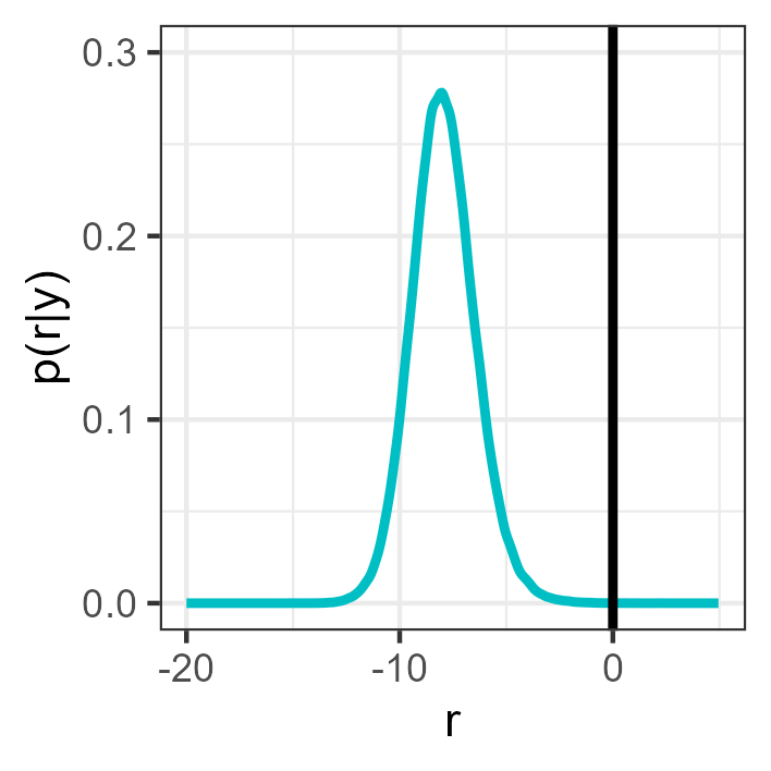
(c)

Figure 2: PDFs of the quantity of interest $R$ in the three illustrative examples: (a) The dose response in Section 3.1, (b) the four-branch function in Section 3.2 and (c) the difference between load and capacity in Section 3.3 ($n_{C}=10$). The vertical lines show the different critical thresholds $T$ targeted within $\mathbb{P}(\mathcal{R}(\boldsymbol{\theta})\geq T|\boldsymbol{y})$.

3.1 Analytical contamination example

In our first test example, we seek to infer a hypothetical contamination field $\boldsymbol{\theta}$ using cell measurements $\boldsymbol{y}$ and aim at predicting the probability of a resulting dose response $\mathcal{R}(\boldsymbol{\theta})$ being critically high for organisms living in the soil. We consider a setting with $M=9$ contamination cells. The “true” values of the contamination level are sampled using independent Gaussian PDFs $\theta_{m}\sim\mathcal{N}(1,0.3^{2})$. For the data $\boldsymbol{y}$, we measure the concentration of the contamination in three cells and assume independent Gaussian observation errors with a standard deviation of $0.05$. We target the quantity of interest $\mathcal{R}(\boldsymbol{\theta})=\sum_{m=1}^{M}\theta_{m}^{2}$, which is related to the linear quadratic dose response (e.g., McMahon 2018). We assume that a dose response that is greater or equal than 20 is critical for the organisms in the soil and aim to estimate $\mathbb{P}(\mathcal{R}(\boldsymbol{\theta})\geq 20.0|\boldsymbol{y})$. As the prior and the likelihood are Gaussian and the measurements depend linearly on the property field $\boldsymbol{\theta}$, there exists an analytical solution for the Gaussian posterior $p_{\boldsymbol{\theta}|\boldsymbol{Y}}(\boldsymbol{\theta}|\boldsymbol{y})$. The PDF $p_{R|\boldsymbol{Y}}(r|\boldsymbol{y})$ of the quantity of interest follows a generalized chi-square distribution (Fig. 2(a)). Even if this distribution does not have a simple closed-form expression, we can derive numerically the true probability of the considered rare event, which is $\mathbb{P}(\mathcal{R}(\boldsymbol{\theta})\geq 20.0|\boldsymbol{y})=1.76\times 10^{-6}$.

We parameterize the bias potential $V_{\psi}(r)$ using RBFs with squared exponential kernels (Eq. 9). We assume a constant shape parameter $\kappa$, use evenly distributed centers $b_{j}$ from $L_{B}$ to $H_{B}$ and only optimize the weights $w_{j}$ during the optimization of $V_{\psi}(r)$. We choose $L_{B}=-80$ and $H_{B}=120$ to ensure that the optimization of the bias potential is not limited by a too narrow range. After testing different numbers of RBFs $B$ and shape parameters $\kappa$, we choose a parameterization with $B=500$ and $\kappa=1$. We also explore our non-parametric approach for modeling the bias potential (Section 2.2.2), which involves employing a kernel density estimate to approximate the probability density function $p_{V}(r)$. To perform this estimation, we utilize the R function density (R Core Team, 2021) with the ‘nrd’ bandwidth configuration (Scott, 2015). In practice, for numerical evaluations, we discretize the function by considering equidistant points within the range of -80 to 120, with a spacing of 0.1.

We introduce a base scenario for the algorithmic setting. For $p_{\textup{ref}}(r)$, we use a Gaussian PDF $\mathcal{N}(20,7^{2})$ centered on the critical threshold. We iterate for a maximum of 500 SGDM optimization steps employing a constant learning rate $\gamma$ of 1.2 and a momentum weight $\beta$ of 0.5 for the RBF parameterization (Eq. 10). For the non-parametric form of the bias potential, we use the same momentum weight and a constant learning rate of 15. For the sampling of $s_{i}\sim p_{V_{\psi}}(\cdot)$ (Eq. 13), we use MH steps employing Gaussian proposals with a step width chosen by initial testing to obtain an acceptance rate close to 30 $\%$. To account for the fact that the posterior is much better defined for the cells where measurements have been made, we adjust the step size for these specific cells. We utilize the KSD stopping criterion with a significance level of $\alpha=95\%$ and a bootstrap parameter $a_{BS}=0.4$ (Section 2.2.3). Following the recommendations of Chwialkowski et al. (2016), we use $n=125$ final samples with a thinning factor of $th=10$ and a burn-in of 100 steps.

First, we examine various choices of $p_{\textup{ref}}(r)$ based on Gaussian distributions $\mathcal{N}(20,\sigma^{2})$, where the standard deviation $\sigma$ ranges from 5 to 8. Figure 3(a) depicts the range of rare event probability estimates obtained from 50 runs using the different choices of $p_{\textup{ref}}(r)$ and both the RBF and the non-parametric estimation of the bias potential. For both forms, the stability and accuracy of the method becomes apparent from a standard deviation of 7 and above. The black points in Figure 3(a) depict the mean probability values of the 50 runs. We observe a positive bias that diminishes as the standard deviation of $p_{\textup{ref}}(r)$ increases. This bias in the estimate is more pronounced for the RBF bias potential. This is a consequence of initializing $V(r)$ as a constant function. During the optimization, the weights of the RBF $V(r)$ are only updated up to a value where samples of $p_{\textup{ref}}(r)$ are located. For $r$ larger than a high quantile of $p_{\textup{ref}}(r)$, the resulting optimized bias potential is biased upwards. Accordingly, $F(r)=-\log(p_{\textup{ref}}(r))-V_{\textup{opt}}(r)$ is too small in that region. This results in $p_{R|\boldsymbol{Y}}(r|\boldsymbol{y})$ and $\mathbb{P}(\mathcal{R}(\boldsymbol{\theta})\geq T|\boldsymbol{y})$ being too large. This effect is less pronounced with the non-parametric bias potential, as the stochastic gradient is based on the analytical PDF $p_{\textup{ref}}(r)$. Figure 3(b) illustrates the minimum and maximum number of forward simulations used in the 50 runs. Despite the stability of the probability estimate’s uncertainty from a standard deviation of 7, the number of required optimization steps continues to rise as the standard deviation increases. The RBF parameterization demands a greater number of simulations compared to the non-parametric approach and yields estimates with a lower variance.

(a)

(b)

Figure 3: Analytical contamination example. (a) Range of rare event probability estimates obtained from 50 EBM runs using different standard deviations in defining $p_{\textup{ref}}(r)$, as well as parametric and non-parametric forms of the bias potential, (b) the corresponding minimum and maximum number of forward simulations. The horizontal line in (a) indicates the true rare event probability and the dots the mean of the 50 estimates.

We now focus on the optimization scheme while maintaining $p_{\textup{ref}}(r)=\mathcal{N}(20,7^{2})$ and the non-parametric form of the bias potential. Figures 4(a) - 4(d) show exemplary trajectories of the Kullback–Leibler divergence, KSD values and rare event probability estimates for different learning rates $\gamma$ and momentum weights $\beta$. We perform 200 optimization steps without any stopping criterion and illustrate the step at which the KSD criteria would have halted the optimization process (indicated by vertical lines). We emphasize that while the Kullback–Leibler divergence exhibits a great amount of scatter, the KSD values demonstrate a much clearer convergence (Figs. 4(a) and 4(b)). The mean, root-mean-square-error (RMSE) and coefficient of variation (COV) of the estimates using a learning rate $\gamma=15$ and momentum weight $\beta=0.5$ are summarized in Table 1. It is observed that whether a stopping criterion is applied or not, the accuracy of the estimate is similar. However, the computational budget can be reduced by almost a factor of 4 when considering 200 fixed optimization steps. Increasing the learning rate comes with a trade-off: while it reduces the computational requirement by reducing the number of optimization steps needed, there is a corresponding loss in accuracy (Fig. 4(c)). The momentum weight plays a crucial role in mitigating the impact of stochastic gradient fluctuations. However, when paired with a too high learning rate, there is a risk of overshooting, necessitating careful adjustment of the learning rate for optimal performance (Fig. 4(d), further discussed in Section 3.3).

(a)

(b)

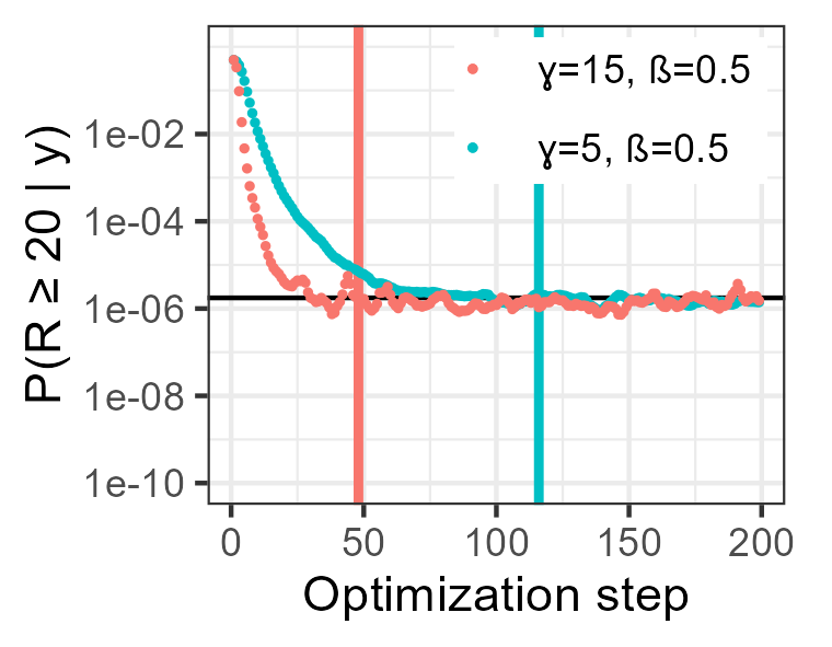
(c)

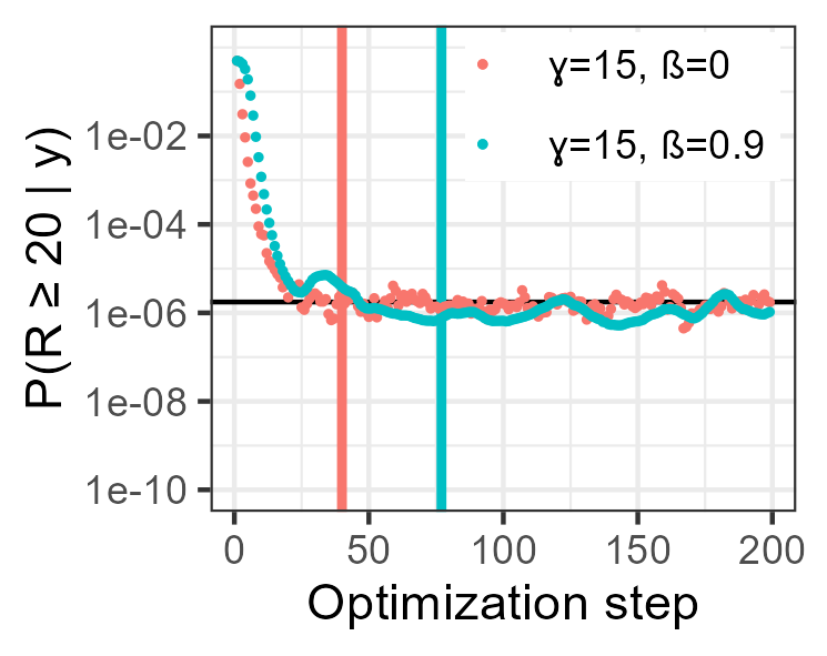
(d)

Figure 4: Analytical contamination example. Exemplary trajectories for the evolving (a) Kullback–Leibler divergence, (b) KSD and (c, d) rare event probability estimate using different learning rates $\gamma$ and momentum weights $\beta$. The horizontal lines in (c, d) indicate the true rare event probability and the vertical lines in (b, c, d) the step at which the KSD criteria would have halted the optimization process.

We compare the results of the EBM method with subset sampling (Section 2.3.1). To perform subset sampling, we establish a fixed burn-in of 100 steps during the initial posterior estimation process. Additionally, we utilize a thinning factor of 500 for the MH samples to promote an initial sample representation that is free from correlation. To prevent bias from an adaptive sequence of thresholds and avoid re-running the algorithm, we use a fixed sequence of thresholds given by a logarithmic function increasing from 5.0 to $T$ within $nr_{t}$ steps. Then we assume the same total computational budget as for the EBM method (including the posterior sampling) and choose the number of samples per subset such as the number of MH steps per subset based on the lowest RMSE using 50 test runs. Here, we choose 60 samples per subset that are each propagated using 20 MH steps. The statistics of the resulting rare event probability estimates are summarized in Table 1. Both the lowest RMSE and COV values obtained with subset sampling are about 60 $\%$ higher than the ones of our EBM approach.

Table 1: Comparison of the EBM method and subset sampling for the analytical contamination example. Mean refers to the mean of the 50 estimates of $\mathbb{P}(\mathcal{R}(\boldsymbol{\theta})\geq T|\boldsymbol{y})$, RSME to their root-mean-square-error and COV to the coefficient of variation. The budget noted for EBM is equal to the mean budget.

Method	Budget	Mean	RMSE	COV
EBM (Stopping criterion)	72 k	$1.74\times 10^{-6}$	$0.62\times 10^{-6}$	0.36
EBM (200 iterations)	270 k	$1.79\times 10^{-6}$	$0.62\times 10^{-6}$	0.35
Subset sampling	72 k	$1.73\times 10^{-6}$	$1.00\times 0^{-6}$	0.58

3.2 Four-branch function

The four-branch function represents a widely used benchmark in structural reliability analysis, characterizing the failure of a system comprising four distinct component limit states (e.g., Schöbi et al. 2017). It is used here to demonstrate the applicability of our EBM method outside of an inversion setting. The four-branch function is defined as,

$$\mathcal{R}(\boldsymbol{\theta})=\min\left\{\begin{array}[]{l}3+0.1(\theta_{1}-\theta_{2})^{2}-\frac{\theta_{1}+\theta_{2}}{\sqrt{2}}\\ 3+0.1(\theta_{1}-\theta_{2})^{2}+\frac{\theta_{1}+\theta_{2}}{\sqrt{2}}\\ (\theta_{1}-\theta_{2})+\frac{6}{\sqrt{2}}\\ (\theta_{2}-\theta_{1})+\frac{6}{\sqrt{2}}\\ \end{array}\right\},$$ (22)

with input variables $\boldsymbol{\theta}=(\theta_{1},\theta_{2})$, which are modeled by two independent standard normally-distributed variables. The traditional rare probability of interest is $\mathbb{P}(\mathcal{R}(\boldsymbol{\theta})\leq T^{*})=\mathbb{P}(-\mathcal{R}(\boldsymbol{\theta})\geq T^{*})$, with $T^{*}=0$. Given that with probability $4.46\times 10^{-3}$ (according to a MC estimation with $10^{8}$ samples in Schöbi et al. 2017) this is not a particularly rare event, we also direct our focus towards $\mathbb{P}(-\mathcal{R}(\boldsymbol{\theta})\geq T^{**})$ with $T^{**}=2$. The distribution of the quantity of interest $R=-\mathcal{R}(\boldsymbol{\theta})$ is depicted in Figure 2(b) and the limit states $\boldsymbol{\theta}$ with $\mathcal{R}(\boldsymbol{\theta})=T^{*}$ are depicted in Figure 5b-d as black outlines.

We use the non-parametric form of the bias potential with the same Gaussian kernel density estimate as in the previous section. As evaluation points, we employ equally-spaced intervals between -10 and 100 with a spacing of 0.1. Our objective is to investigate the performance of the EBM method under a restricted computational budget of 10,000 evaluations. To perform the sampling of $s_{i}\sim p_{V_{\psi}}(\cdot)$, we use MH steps with Gaussian proposals aiming for an acceptance rate close to 30 $\%$. We test a configuration using a stopping criterion employing a significance level of $\alpha=0.99$ and $a_{BS}=0.5$. With an appropriate thinning factor (4) and burn-in period (5 steps), this results in 100 samples obtained during 405 MH iterations. We run the EBM process with a constant learning rate of $\gamma=6.5$ and momentum weight $\beta=0.5$.

The optimized bias potential $V_{\textup{opt}}(r)$ takes on different forms depending on the chosen PDF $p_{\textup{ref}}(r)$, impacting not only $p_{V_{\textup{opt}}}(r)$, but also $p_{V_{\textup{opt}}}(\boldsymbol{\theta})$ (Eq. 14), which has to be explored by MH steps to obtain the samples $s_{i}\sim p_{V_{\psi}}(\cdot)$. This is particularly interesting in this test example, as the failure event is connected to four distinct regions of the parameter space. Figure 5 shows samples of the resulting joint PDFs $p_{V_{\textup{opt}}}(\theta_{1},\theta_{2})$ for different choices of $p_{\textup{ref}}(r)$ together with the limit states $\boldsymbol{\theta}$ with $\mathcal{R}(\boldsymbol{\theta})=T^{*}$ (black outlines). The corresponding means and COVs for the rare event probability estimates are shown in Table 2. We start with a Gaussian distribution centred on the first threshold of interest, $\mathcal{N}(0,2^{2})$. The resulting joint PDF $p_{V_{\textup{opt}}}(\theta_{1},\theta_{2})$ (Fig. 5(b)) appears to be relatively compact and only explores a small part of the area outside the limit states. This leads to a high mean estimate (Table 2). Merely increasing the standard deviation means that $p_{\textup{ref}}(r)$ also puts high mass on the left tails of the distribution of $R$, a wasteful allocation of resources.

As an alternative, we consider an asymmetric and heavy -tailed Generalized Extreme Value (GEV) distribution as $p_{\textup{ref}}(r)$. We start with $\mathrm{GEV}(2,2,0.33)$ using a location parameter of 2, a scale parameter of 2, and a shape parameter of 0.33. This shift results in a PDF $p_{\textup{ref}}(r)$ that has minimal mass in the high-probability region of $R$ (Fig. 5(a)). The resulting joint PDF $p_{V_{\textup{opt}}}(\theta_{1},\theta_{2})$ (Fig. 5(c)) displays an increased level of exploration outside the limit states but partly omits the central region that links the four branches. This creates challenges when transitioning between modes during the MH sampling process, leading to biased probability estimates with high COVs (Table 2). These findings suggest that a well-chosen $p_{\textup{ref}}(r)$ should not only have heavy right tails, but also include the high probability region of $R$ while excluding the left tails of its distribution. Therefore, we change to a type I extreme value distribution $\mathrm{GEV}(2,3,0)$ (Fig. 5(a)), which expands the joint PDF $p_{V_{\textup{opt}}}(\theta_{1},\theta_{2})$ while the central region is still incorporated (Fig. 5(d)). Consequently, our results yield a mean probability estimate for $T^{*}$ that aligns with the one in Schöbi et al. (2017). Moreover, for $T^{**}$, we observe a significantly reduced mean compared to the alternative $p_{\textup{ref}}(r)$, and for both thresholds, the COVs are at their lowest with the latter choice.

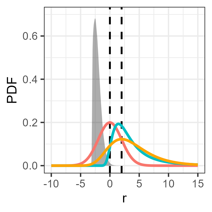
(a)

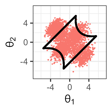
(b)

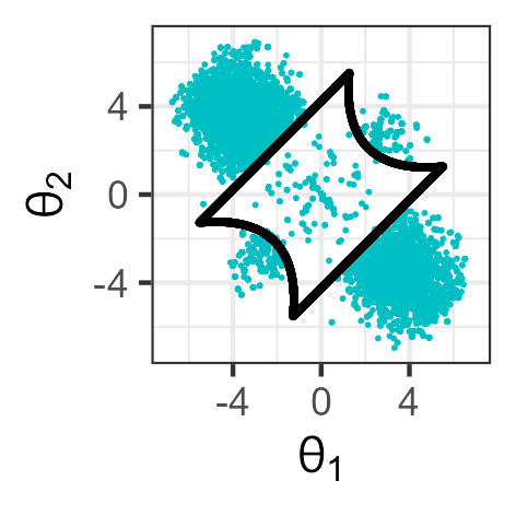
(c)

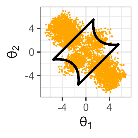
(d)

Figure 5: Impact of $p_{\textup{ref}}(r)$ for the four-branch function example. (a) Distribution of the quantity of interest $R$ (filled) with two considered thresholds (dashed vertical), along with the PDFs $\mathcal{N}(0,2^{2})$ (red), $\mathrm{GEV}(2,2,0.33)$ (blue) and $\mathrm{GEV}(2,3,0)$ (orange). A total of 10,000 samples of the resulting trained $p_{V}(\theta_{1},\theta_{2})$ obtained with (b) $\mathcal{N}(0,2^{2})$, (c) $\mathrm{GEV}(2,2,0.33)$, and (d) $\mathrm{GEV}(2,3,0)$. The black outlines in (b, c, d) depict the limit states $\boldsymbol{\theta}$ with $\mathcal{R}(\boldsymbol{\theta})=T^{*}$.

To ensure a connected $p_{V_{\textup{opt}}}(\theta_{1},\theta_{2})$ and enhanced exploration of the failure regions, we consider $\mathrm{GEV}(2,3,0)$ to be the best choice. In evaluating subset sampling for comparison purposes, we employ the average computational budget of the EBM approach. A satisfactory performance was achieved with 80 samples per subset and a propagation using 5 MH steps. For both thresholds, we obtain comparable mean estimates with both methods, yet higher COVs with subset sampling compared to EBM with $\mathrm{GEV}(2,3,0)$. In fact, the COV for the second threshold $T^{**}$ is about 50 $\%$ higher.

Table 2: Comparison of the EBM method and subset sampling for the four-branch example. Mean refers to the mean of the 50 estimates of $\mathbb{P}(-\mathcal{R}(\boldsymbol{\theta})\geq T)$ for the two thresholds $T^{*}$ and $T^{**}$ and COV to the coefficient of variation. The budget noted for EBM is equal to the mean budget. The Monte Carlo results for $T^{*}$ are copied from Schöbi et al. (2017).

Method	$p_{\textup{ref}}(r)$	Budget	Mean $T^{*}$	COV $T^{*}$	Mean $T^{**}$	COV $T^{**}$
MC	-	$10^{5}$ k	$4.46\times 10^{-3}$	0.0015	-	-
EBM	$\mathcal{N}(0,2^{2})$	5 k	$5.79\times 10^{-3}$	0.47	$45.69\times 10^{-5}$	0.63
EBM	$\mathrm{GEV}(2,2,0.33)$	12 k	$82.45\times 10^{-3}$	1.63	$31.29\times 10^{-5}$	1.09
EBM	$\mathrm{GEV}(2,3,0)$	10 k	$4.97\times 10^{-3}$	0.31	$1.56\times 10^{-5}$	0.53
Subset sampling	-	10 k	$4.91\times 10^{-3}$	0.36	$1.36\times 10^{-5}$	0.80

3.3 Load capacity example

As a third test case, we consider the load capacity example of Straub et al. (2016), enabling comparison of our EBM approach with their BUS method (Section 2.3.2). The problem under consideration is a basic reliability problem concerned with the failure of an engineering system when the load $\boldsymbol{\theta}^{L}$ exceeds the capacity $\boldsymbol{\theta}^{C}$. The corresponding rare event probability of interest is,

$$\mathbb{P}(\mathcal{R}(\boldsymbol{\theta})\geq 0)=\mathbb{P}(\boldsymbol{\theta}^{L}-\boldsymbol{\theta}^{C}\geq 0),$$ (23)

with $\boldsymbol{\theta}=(\boldsymbol{\theta}^{L},\boldsymbol{\theta}^{C})$. For the load $\boldsymbol{\theta}^{L}$, we assume a prior Gumbel distribution with mean 2 and standard deviation 1 and the capacity $\boldsymbol{\theta}^{C}$ is lognormal distributed with mean 12 and standard deviation 2; the variables are assumed to be independent. To investigate the performance for a problem with increasing number of model parameters, Straub et al. (2016) express the capacity as a product of component capacities $\boldsymbol{\theta}^{C}_{i}$ ($1\leq i\leq n_{C}$). The component capacities $\boldsymbol{\theta}^{C}_{i}$ follow a lognormal distribution such that $\boldsymbol{\theta}^{C}$ still has mean 12 and standard deviation 2.

In this inversion setting, individual measurements $y_{i}$ of the component capacities $\boldsymbol{\theta}^{C}_{i}$ are considered. To ensure analytical solutions, multiplicative lognormal measurement errors,

$$p_{\boldsymbol{Y}|\boldsymbol{\theta}}(\boldsymbol{y}|\boldsymbol{\theta})=p(\boldsymbol{y}|\boldsymbol{\theta}^{C}_{1},\boldsymbol{\theta}^{C}_{2},...,\boldsymbol{\theta}^{C}_{n_{C}})\propto\exp\left(-\frac{1}{2}\sum_{i=1}^{n_{C}}\left(\frac{\log y_{i}-\log\boldsymbol{\theta}^{C}_{i}}{\sigma_{y}}\right)^{2}\right),$$ (24)

with $\sigma_{y}=0.05$ and $y_{i}=8^{1/n_{C}}$ are employed. Following Straub et al. (2016), we consider $n_{C}=10$ and $n_{C}=100$ with the resulting failure probabilities $\mathbb{P}(\boldsymbol{\theta}^{L}-\boldsymbol{\theta}^{C}\geq 0|\boldsymbol{y})$ being $6.8\times 10^{-5}$ and $2.1\times 10^{-5}$, respectively. The posterior distribution of $R=\mathcal{R}(\boldsymbol{\theta})=\boldsymbol{\theta}^{L}-\boldsymbol{\theta}^{C}$ for $n_{C}=10$ with the critical threshold of $T=0$ is depicted in Figure 2(c).

The results of the BUS approach with subset sampling are reproduced in Table 3. As Straub et al. (2016), we transform the reliability problem to the standard normal space by marginal transformations of the load and capacity variables. To enable a direct comparison of the EBM with the BUS approach, we employ the same computational budgets. In order to accommodate a consistent and constrained computational budget in the context of EBM, we use a fixed number of optimizations steps (no stopping criterion). Following our analysis in the previous section, we employ as $p_{\textup{ref}}(r)$ a type I extreme value distribution $\mathrm{GEV}(0,7,0)$. To make the method dimensionally robust, we use prior-preserving preconditioned Crank-Nicolson proposals (pCN; e.g. Cotter et al. 2013) within the sampling of $s_{i}\sim p_{V_{\psi}}(\cdot)$. Then, we use a burn-in of 10 steps, a thinning factor of $th=6$ and $a_{BS}=0.5$. As we do not rely on a stopping criterion, we further divide the number of final samples by a factor of two (Chwialkowski et al., 2016), leading to $n=50$ obtained by 310 MH steps. Then we fix the number of optimization steps in accordance with the computational budget (resulting in 25 and 27 steps for the two values of $n_{C}$).

We test both a parametric and non-parametric form for the bias potential. For the parametric approach, we employ RBFs with squared exponential kernels (Eq. 9), using $L_{B}=-100$ and $H_{B}=100$, $B=500$ and $\kappa=0.5$. We run the EBM process with an exponentially decreasing learning rate initiated as $\gamma=0.5$ (factor -0.005) and momentum weight $\beta=0.5$. For the non-parametric form, we use the same Gaussian kernel density estimate of $p_{V}(r)$ as in the previous sections and evaluation points between -100 and 100 with a spacing of 0.1. Here we employ an exponentially decreasing learning rate initiated as $\gamma=19$ (factor -0.005) and momentum weight $\beta=0.95$. The means and 95 $\%$ confidence intervals of 50 runs are shown in Table 3 and the corresponding estimates of $V(r)$ are depicted in Figure 6(a) for the RBFs and in Figure 6(b) for the non-parametric form. With a non-parametric $V(r)$, we sometimes obtain bias potentials characterized by minor-scale fluctuations, in contrast to the smoother bias potentials generated by RBFs, which exhibit more pronounced large-scale fluctuations. The small-scale fluctuations arise due to the constraints of our limited computational resources, compelling us to base the kernel density estimates on a relatively small set of samples, which may not be adequately thinned. To mitigate this issue and promote a smoother estimation, we have increased the momentum weight to $\beta=0.95$. However, this adjustment also introduces challenges in fine-tuning the learning process, as it tends to cause overshooting during optimization. Due to the changed PDF $p_{R|\boldsymbol{Y}}(r|\boldsymbol{y})$ and computational budget for $n_{C}=100$, we have to adapt the learning rate schedule for an optimal performance and use $\gamma=22$ and a decay factor of -0.003. On the other hand, the RBF parameterization with lower momentum weight is less sensitive to the choice of the learning rate schedule and we can use the same for both scenarios. For both $n_{C}$, both presented configurations of the EBM approach lead to a reduction of the 95 $\%$ confidence interval’s length compared to the BUS approach. While the non-parametric form, when coupled with a higher momentum weight, yields noticeably increased accuracy, it also becomes significantly more sensitive to the learning rate schedule.

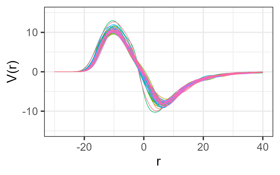
(a)

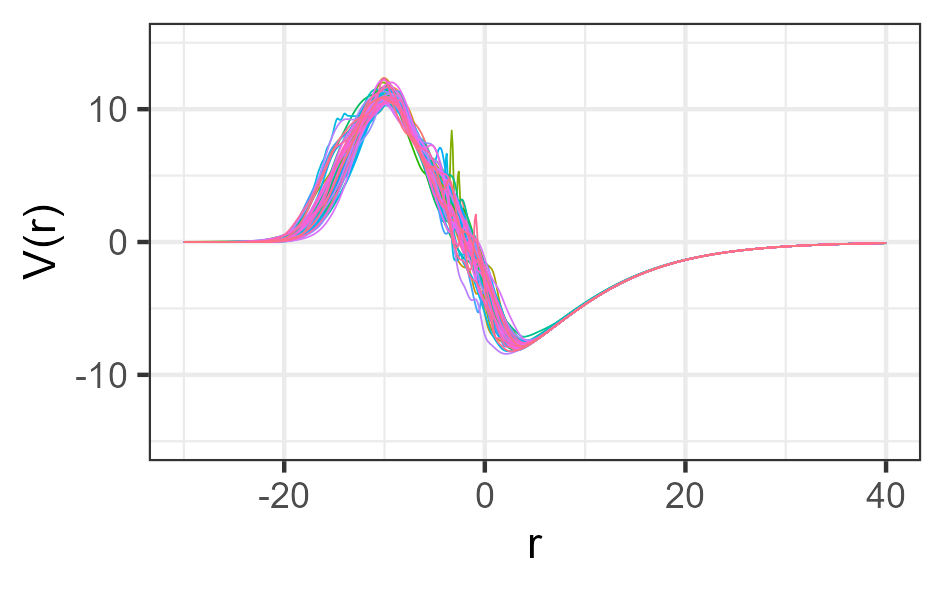
(b)

Figure 6: Twenty optimized bias potentials $V(r)$ for the load capacity example ($n_{C}=100$) using (a) the RBF parameterization and (b) the non-parametric form.

Table 3: Table summarizing the comparison of EBM and BUS for the load capacity example. The 95 $\%$ confidence intervals of the BUS method with subset sampling are copied from Straub et al. (2016), the mean value is not provided.

Case	Method	Budget	Mean	95 $\%$ confidence interval
$n_{C}=10$	Analytical	-	$6.8\times 10^{-5}$	-
	EBM (non-par.)	7.7 k	$7.0\times 10^{-5}$	$[2.7,12.0]\times 10^{-5}$
	EBM (RBF)	7.7 k	$7.1\times 10^{-5}$	$[0.9,19.5]\times 10^{-5}$
	BUS	7.7 k	-	$[2.1,35.0]\times 10^{-5}$
$n_{C}=100$	Analytical	-	$2.1\times 10^{-5}$	-
	EBM (non-par.)	12.6 k	$2.7\times 10^{-5}$	$[1.2,4.7]\times 10^{-5}$
	EBM (RBF)	8.4 k	$4.0\times 10^{-5}$	$[0.3,10.0]\times 10^{-5}$
	BUS	8.4 k	-	$[0.2,12.0]\times 10^{-5}$

4 Discussion

This paper presents a novel energy-based model (EBM) approach for estimating probabilities of rare events that is applicable not only for conventional rare event estimation but also in inversion settings. The approach centers on representing the distribution of the quantity of interest as an energy density function. The estimation of the related free energy is achieved by optimizing a bias potential, aligning it with a predefined distribution $p_{\textup{ref}}(r)$ that has most mass on the region of interest.

When parameterizing the bias potential $V_{\psi}(r)$, it is crucial to allow for an appropriate amount of flexibility. We recommend to compare results obtained by a chosen parameterization with those obtained with a more flexible parameterization. An alternative approach is to use a non-parametric form for the bias potential $V(r)$. Depending on the test case and the computational budget, we illustrate the effectiveness of the non-parametric bias potential in alleviating bias issues and reducing computational needs (Fig. 3). However, the non-parametric approach relies heavily on the quality of the kernel density estimate used during the optimization. In cases where computational resources are limited, and when dealing with correlated samples, it is possible to obtain bias potentials that exhibit fine-scale fluctuations resulting from individual optimization steps (Fig. 6(b)). A parameterization, on the other hand, does not face this problem as it can be chosen such that it enforces a smooth bias potential (Fig. 6(a)). However, when opting for a parameterization, we face the critical decision of choosing the appropriate form, which can significantly impact the final outcomes. When manually fine-tuning the bandwidth of the kernel density estimate within the non-parametric approach, we also retain the capability to shape the potential’s form, but this comes at the cost of introducing additional configuration choices.

When selecting the distribution $p_{\textup{ref}}(r)$, one needs to consider that too light right tails lead to a positive bias in the estimates of $\mathbb{P}(\mathcal{R}(\boldsymbol{\theta})\geq T|\boldsymbol{y})$. This effect is the most pronounced for the parametric approach, as the optimization relies on samples of $p_{\textup{ref}}(r)$ and $p_{V}(r)$. Beyond a certain quantile, the probability of obtaining samples is extremely small, leading to an overestimation of $V(r)$ in this region (under the assumption that the initial potential is constant everywhere). The same principle would hold for $\mathbb{P}(\mathcal{R}(\boldsymbol{\theta})\leq T|\boldsymbol{y})$ and the left tails of $p_{\textup{ref}}(r)$. Since our primary focus is on failure probability estimates, a slight positive bias in the probability value is not too problematic. Additionally, the non-parametric form reduces this bias as the optimization relies on PDFs enabling an integration of the tails. The choice of $p_{\textup{ref}}(r)$ also determines the form of the PDF $p_{V}(\boldsymbol{\theta})$ (Eq. 14), which needs to be explored by MH in each optimization step. In the second test example utilizing the four-branch function (Section 3.2), we showcase the benefit of using an asymmetric Generalized Extreme Value (GEV) distribution as $p_{\textup{ref}}(r)$ (Fig. 5). The form of the GEV distribution enables a $p_{\textup{ref}}(r)$ with heavy right tails that includes the high probability region of $R$. For this example with distinct regions contributing to the rare event, the incorporation of the region of high probability of the quantity of interest within $p_{\textup{ref}}(r)$ facilitates the MH algorithm’s ability to shift between the modes, leading to a lower coefficient of variation in the probability estimates.

We optimize the bias potential using stochastic gradient descent with momentum. Regarding the learning rate, a smaller value tends to lead to more stable estimates but also to a larger number of optimization steps (Fig. 4). Conversely, higher learning rates result in increased fluctuations but require fewer steps for convergence. The momentum has the advantage of dampening oscillations in the convergence process and making it more robust to noisy gradients, however, it requires careful tuning of the learning rate and momentum weight, to achieve optimal performance. Besides stochastic gradient descent with momentum, there exist numerous alternative implementations for the optimization. For instance, for the last test case requiring fine tuning of the optimization schedule (Section 3.3), exploring more advanced optimization algorithms like Adam (Kingma and Ba, 2015) would be interesting. We combine the optimization with a stopping criterion based on a goodness-of-fit test employing the Kernelized Stein discrepancy. This is done as the Kullback–Leibler divergence used in the optimization of the bias potential exhibits a great amount of scatter compared with KSD that demonstrates a much clearer convergence. This characteristic of the KSD makes it a valuable diagnostic tool in determining the appropriate moment to stop the optimization process. This achieves two key benefits: First, it helps stabilize the rare event probability estimates by ensuring that the biased probability distribution $p_{V}(r)$ closely approximates the target probability distribution $p_{\textup{ref}}(r)$. Second, it reduces computational effort by allowing the optimization process to halt as soon as the approximation becomes sufficiently accurate (Fig. 4). To account for the correlation in the samples, we use the specific bootstrap method proposed by Chwialkowski et al. (2016).

We compare the performance of the EBM approach against alternative methods (Section 2.3) using three illustrative test examples. In the first contamination test case involving inversion (Section 3.1), the EBM method outperforms subset sampling, reducing the root-mean-square-error (RMSE) and coefficient of variation (COV) by about 40 $\%$ (Table 1). In the second example involving the four-branch function (Section 3.2), subset sampling also exhibits poorer performance than the EBM approach, with the latter reducing the COV by up to 35 $\%$ compared to subset sampling. In the third example in Section 3.3, we compare the EBM method’s performance against the BUS approach with subset sampling in a simplistic engineering test case from Straub et al. (2016). For both numbers of considered capacity components, the EBM method is able to narrow down the 95 $\%$ confidence interval compared to the BUS approach (Table 3).

Regarding different approaches for sampling $s_{i}\sim p_{V_{\psi}}(\cdot)$, we experiment with various bootstrap parameters $a_{BS}$ (results not shown). We notice that there is an increase in the variance of the probability estimates with growing $a_{BS}$. However, the reduced values for small bootstrap parameters come at the expense of a higher number of forward simulations. Similar to the learning rate, there seems to be a trade-off between computational cost and accuracy. Besides testing other parameterizations for $V(r)$, distributions for $p_{\textup{ref}}(r)$ and optimization schemes for updating $V(r)$, one could also consider replacing the sampler for $p_{V}(\boldsymbol{\theta})$. For instance, other proposal schemes, interacting MH chains or a particle method could be considered (e.g., Robert et al. 2018). In data rich settings with narrow posterior distributions, it is expected that $V(r)$ will vary over very large ranges. In such scenarios, it could be beneficial to know in advance the expected properties of $V(r)$ such as shape, smoothness class and range. This could potentially be achieved by using a simplistic free energy function estimate (e.g. histogram based) of some thousands of posterior samples giving together with $p_{\textup{ref}}(r)$ to obtain a first approximation of $V_{\mathrm{opt}}(r)$.

5 Conclusion

This paper introduces an energy-based model (EBM) approach to estimate rare event probabilities. The approach is based on formulating the distribution of the quantity of interest as an energy density function with a corresponding free energy function. By optimizing a bias potential such that the corresponding energy density approaches a pre-defined PDF $p_{\textup{ref}}(r)$, the method estimates the free energy accurately in the region targeted by $p_{\textup{ref}}(r)$. The presented approach is applicable both for traditional rare event estimation and in the context of inversion settings when one is not interested in the posterior itself, but rather in the distribution of a quantity that depends on the posterior. When employed in such a setting, this formulation reduces the potentially high-dimensional problem of first estimating the posterior and subsequently the quantity of interest to the optimization of a one-dimensional function. The optimization of the bias potential involves minimizing the Kullback–Leibler divergence and a stopping criterion based on the Kernelized Stein Discrepancy is introduced to terminate the optimization process. The stopping criterion not only enhances the stability and accuracy of the rare event probability estimation but also optimizes computational resources by terminating the optimization process when the approximation is deemed satisfactory. A non-parametric form of the bias potential is introduced, which eliminates the need to make a parameterization choice while simultaneously enabling efficient and accurate probability estimates. For the three presented exemplary test cases, a properly configured EBM approach ensures precise estimations of rare event probabilities and outperforms the examined variants of subset sampling methods.

Appendix A Relation to maximum likelihood estimation

We can reformulate the minimization of the Kullback-Leibler divergence as a maximum likelihood estimation problem. While we summarize the general concepts and implications of this relation, we refer to Van der Vaart (2000) for the theoretical details about maximum likelihood estimation.

Let $R$ be a random variable, whose distribution $P$ has a PDF $p_{V_{\psi}}(r)$ with a statistical model $\{p_{V_{\psi}}(\cdot):\psi\in\Psi\}$. Furthermore, $r_{i}$ for $1\leq i\leq n$ are $n$ independently generated realizations of $R$. The log-likelihood function of the model is given by,

$$l_{n}(\psi)=\log\prod_{i=1}^{n}p_{V_{\psi}}(r_{i})=\sum_{i=1}^{n}\log p_{V_{\psi}}(r_{i}).$$ (25)

A maximum likelihood estimator (MLE) is defined as $\hat{\psi}_{MLE}\in\Psi$ with $l_{n}(\hat{\psi}_{MLE})=\underset{\psi\in\Psi}{\max}\hskip 5.69046ptl_{n}(\psi)$.

We define,

$$\ell(\psi):=\mathbb{E}_{\psi_{0}}(\log p_{V_{\psi}}(R))=\int\log p_{V_{\psi}}(r)p_{V_{\psi_{0}}}(r)\mathrm{d}r.$$ (26)

Under the assumption that the model is well specified with $p_{V_{\psi_{0}}}(r)$ being the PDF of $P$ and $\mathbb{E}(|\log p_{V_{\psi}}(R)|)<\infty$, $\psi\mapsto\ell(\psi)$ is maximized at $\psi_{0}$. The normalized log-likelihood $\psi\mapsto\frac{1}{n}l_{n}(\psi)$ is a sample approximation of $\psi\mapsto\ell(\psi)$, and under some regularity constraints, $\frac{1}{n}\l_{n}(\psi)\overset{a.s.}{\longrightarrow}\mathbb{E}_{\psi_{0}}\large(\log p_{V_{\psi}}(R)\large)$ almost surely such that the MLE $\hat{\psi}_{MLE}$ is a consistent estimator for $\psi_{0}$. Furthermore, under some additional conditions, the MLE follows asymptotic normality,

$$\sqrt{n}(\hat{\psi}_{MLE}-\psi_{0})\overset{d}{\longrightarrow}\mathcal{N}(0,I(\psi_{0})^{-1}),\quad\text{for }n\rightarrow\infty,$$ (27)

with the Fisher information matrix $I(\psi_{0})=\mathbb{E}_{\psi_{0}}\Big{(}\nabla_{\psi}\log p_{V_{\psi}}(R)\nabla_{\psi}\log p_{V_{\psi}}(R)^{T}\Big{)}$.

In our setting, we assume that $p_{\textup{ref}}(r)=p_{V_{\psi_{0}}}(r)$ for $\psi_{0}\in\Psi$. Furthermore, the Kullback-Leibler divergence between two distributions with PDFs $p_{V_{\psi}}(\cdot)$ and $p_{V_{\psi_{0}}}(\cdot)$ can be expressed as $\ell(\psi_{0})-\ell(\psi)$:

$$\textup{KL}(p_{V_{\psi_{0}}}||p_{V_{\psi}})=\int\log p_{V_{\psi_{0}}}(r)p_{V_{\psi_{0}}}(r)\mathrm{d}r-\int\log p_{V_{\psi}}(r)p_{V_{\psi_{0}}}(r)\mathrm{d}r.$$ (28)

The reformulation $\ell(\psi)=\ell(\psi_{0})-\textup{KL}(p_{V_{\psi_{0}}}||p_{V_{\psi}})$ shows that maximizing the likelihood is equal to minimizing the Kullback-Leibler divergence.

Acknowledgements

This work was supported by the Swiss National Science Foundation (project number: 184574).

References

References

- Au and Beck (1999) S.-K. Au and J. L. Beck. A new adaptive importance sampling scheme for reliability calculations. Structural Safety, 21(2):135–158, 1999.
- Au and Beck (2001) S.-K. Au and J. L. Beck. Estimation of small failure probabilities in high dimensions by subset simulation. Probabilistic Engineering Mechanics, 16(4):263–277, 2001.
- Au and Wang (2014) S.-K. Au and Y. Wang. Engineering Risk Assessment with Subset Simulation. John Wiley & Sons, 2014.
- Beck and Zuev (2015) J. L. Beck and K. M. Zuev. Rare event simulation. In R. Ghanem, D. Higdon, and H. Owhadi, editors, Handbook of Uncertainty Quantification, pages 1–26. Springer, Cham, 2015.
- Betz et al. (2014) W. Betz, I. Papaioannou, and D. Straub. Adaptive variant of the BUS approach to Bayesian updating. In A. Cunha, E. Caetano, P. Ribeiro, and G. Müller, editors, Proceedings of the 9th International Conference on Structural Dynamics, EURODYN 2014, pages 3021–3028, 2014.
- Bonati et al. (2019) L. Bonati, Y.-Y. Zhang, and M. Parrinello. Neural networks-based variationally enhanced sampling. Proceedings of the National Academy of Sciences, 116(36):17641–17647, 2019.
- Bucklew (2004) J. A. Bucklew. Introduction to Rare Event Simulation, volume 5. Springer, New York, 2004.
- Cérou et al. (2012) F. Cérou, P. Del Moral, T. Furon, and A. Guyader. Sequential Monte Carlo for rare event estimation. Statistics and Computing, 22(3):795–808, 2012.
- Chwialkowski et al. (2016) K. Chwialkowski, H. Strathmann, and A. Gretton. A kernel test of goodness of fit. In M. F. Balcan and K. Q. Weinberger, editors, International Conference on Machine Learning, PMLR, pages 2606–2615, 2016.
- Cotter et al. (2013) S. L. Cotter, G. O. Roberts, A. M. Stuart, and D. White. MCMC methods for functions: modifying old algorithms to make them faster. Statistical Science, 28(3):424 – 446, 2013.
- Goodfellow et al. (2016) I. Goodfellow, Y. Bengio, and A. Courville. Deep Learning. MIT press, 2016.
- Gorham and Mackey (2015) J. Gorham and L. Mackey. Measuring sample quality with Stein’s method. In C. Cortes, N. Lawrence, D. Lee, M. Sugiyama, and R. Garnett, editors, Advances in Neural Information Processing Systems 28, NIPS, volume 28, 2015.
- Gorham and Mackey (2017) J. Gorham and L. Mackey. Measuring sample quality with kernels. In D. Precup and Y. W. Teh, editors, International Conference on Machine Learning, PMLR, pages 1292–1301, 2017.
- Hadjidoukas et al. (2015) P. E. Hadjidoukas, P. Angelikopoulos, C. Papadimitriou, and P. Koumoutsakos. 4u: A high performance computing framework for Bayesian uncertainty quantification of complex models. Journal of Computational Physics, 284:1–21, 2015.
- Hasofer and Lind (1974) A. M. Hasofer and N. C. Lind. Exact and invariant second-moment code format. Journal of the Engineering Mechanics Division, 100(1):111–121, 1974.
- Hastings (1970) W. K. Hastings. Monte Carlo sampling methods using Markov chains and their applications. Biometrika, 57(1):97–109, 04 1970. ISSN 0006-3444. doi: 10.1093/biomet/57.1.97. URL https://doi.org/10.1093/biomet/57.1.97.
- Hohenbichler and Rackwitz (1988) M. Hohenbichler and R. Rackwitz. Improvement of second-order reliability estimates by importance sampling. Journal of Engineering Mechanics, 114(12):2195–2199, 1988.
- Invernizzi et al. (2017) M. Invernizzi, O. Valsson, and M. Parrinello. Coarse graining from variationally enhanced sampling applied to the Ginzburg–Landau model. Proceedings of the National Academy of Sciences, 114(13):3370–3374, 2017.
- Jensen et al. (2013) H. Jensen, C. Vergara, C. Papadimitriou, and E. Millas. The use of updated robust reliability measures in stochastic dynamical systems. Computer Methods in Applied Mechanics and Engineering, 267:293–317, 2013.
- Juneja and Shahabuddin (2006) S. Juneja and P. Shahabuddin. Rare-event simulation techniques: an introduction and recent advances. Handbooks in Operations Research and Management Science, 13:291–350, 2006.
- Kanjilal et al. (2023) O. Kanjilal, I. Papaioannou, and D. Straub. Bayesian updating of reliability by cross entropy-based importance sampling. Structural Safety, 102:102325, 2023.
- Kästner and Thiel (2005) J. Kästner and W. Thiel. Bridging the gap between thermodynamic integration and umbrella sampling provides a novel analysis method:“Umbrella integration”. The Journal of Chemical Physics, 123(14):144104, 2005.
- Kingma and Ba (2015) D. P. Kingma and J. Ba. Adam: A method for stochastic optimization. In Y. Bengio and Y. LeCun, editors, 3rd International Conference for Learning Representations, ICLR, Conference Track Proceedings, 2015.
- Koutsourelakis et al. (2004) P.-S. Koutsourelakis, H. J. Pradlwarter, and G. I. Schueller. Reliability of structures in high dimensions, part i: algorithms and applications. Probabilistic Engineering Mechanics, 19(4):409–417, 2004.
- Lelièvre et al. (2010) T. Lelièvre, G. Stoltz, and M. Rousset. Free Energy Computations: A Mathematical Perspective. World Scientific, 2010.
- Liu et al. (2016) Q. Liu, J. Lee, and M. Jordan. A kernelized Stein discrepancy for goodness-of-fit tests. In M. F. Balcan and K. Q. Weinberger, editors, International Conference on Machine Learning, PMLR, pages 276–284, 2016.
- Liu et al. (2020) Y. Liu, Y. Gao, and W. Yin. An improved analysis of stochastic gradient descent with momentum. Advances in Neural Information Processing Systems, 33:18261–18271, 2020.
- McMahon (2018) S. J. McMahon. The linear quadratic model: usage, interpretation and challenges. Physics in Medicine & Biology, 64(1):01TR01, 2018.
- Metropolis et al. (1953) N. Metropolis, A. W. Rosenbluth, M. N. Rosenbluth, A. H. Teller, and E. Teller. Equation of state calculations by fast computing machines. The Journal of Chemical Physics, 21(6):1087–1092, 1953.
- Papadimitriou et al. (2001) C. Papadimitriou, J. L. Beck, and L. S. Katafygiotis. Updating robust reliability using structural test data. Probabilistic Engineering Mechanics, 16(2):103–113, 2001.
- R Core Team (2021) R Core Team. R: A Language and Environment for Statistical Computing. R Foundation for Statistical Computing, Vienna, Austria, 2021. URL https://www.R-project.org/.
- Robert et al. (2018) C. P. Robert, V. Elvira, N. Tawn, and C. Wu. Accelerating mcmc algorithms. Wiley Interdisciplinary Reviews: Computational Statistics, 10(5):e1435, 2018.
- Rubino and Tuffin (2009) G. Rubino and B. Tuffin. Rare Event Simulation Using Monte Carlo Methods. John Wiley & Sons, 2009.
- Schöbi et al. (2017) R. Schöbi, B. Sudret, and S. Marelli. Rare event estimation using polynomial-chaos kriging. ASCE-ASME Journal of Risk and Uncertainty in Engineering Systems, Part A: Civil Engineering, 3(2):D4016002, 2017.
- Scott (2015) D. W. Scott. Multivariate Density Estimation: Theory, Practice, and Visualization. John Wiley & Sons, 2015.
- Shao (2010) X. Shao. The dependent wild bootstrap. Journal of the American Statistical Association, 105(489):218–235, 2010.
- Shirts and Ferguson (2020) M. R. Shirts and A. L. Ferguson. Statistically optimal continuous free energy surfaces from biased simulations and multistate reweighting. Journal of Chemical Theory and Computation, 16(7):4107–4125, 2020.
- Song and Kingma (2021) Y. Song and D. P. Kingma. How to train your energy-based models. arXiv preprint arXiv:2101.03288, 2021.
- Stecher et al. (2014) T. Stecher, N. Bernstein, and G. Csányi. Free energy surface reconstruction from umbrella samples using Gaussian process regression. Journal of Chemical Theory and Computation, 10(9):4079–4097, 2014.
- Stein (1972) C. Stein. A bound for the error in the normal approximation to the distribution of a sum of dependent random variables. In Proceedings of the Sixth Berkeley Symposium on Mathematical Statistics and Probability, Volume 2: Probability Theory, pages 583–602, 1972.
- Straub (2011) D. Straub. Reliability updating with equality information. Probabilistic Engineering Mechanics, 26(2):254–258, 2011.
- Straub and Papaioannou (2015) D. Straub and I. Papaioannou. Bayesian updating with structural reliability methods. Journal of Engineering Mechanics, 141(3):04014134, 2015.
- Straub et al. (2016) D. Straub, I. Papaioannou, and W. Betz. Bayesian analysis of rare events. Journal of Computational Physics, 314:538–556, 2016.
- Sundar and Manohar (2013) V. Sundar and C. Manohar. Updating reliability models of statically loaded instrumented structures. Structural Safety, 40:21–30, 2013.
- Torrie and Valleau (1977) G. M. Torrie and J. P. Valleau. Nonphysical sampling distributions in Monte Carlo free-energy estimation: Umbrella sampling. Journal of Computational Physics, 23(2):187–199, 1977.
- Valsson and Parrinello (2014) O. Valsson and M. Parrinello. Variational approach to enhanced sampling and free energy calculations. Physical Review Letters, 113(9):090601, 2014.
- Van der Vaart (2000) A. W. Van der Vaart. Asymptotic Statistics, volume 3. Cambridge University Press, 2000.
- Wang and Landau (2001) F. Wang and D. P. Landau. Efficient, multiple-range random walk algorithm to calculate the density of states. Physical Review Letters, 86(10):2050, 2001.