AstroSat observation of the magnetar SGR J1830$-$0645 during its first detected X-ray outburst

Abstract

We present here timing and spectral analyses of SGR J1830$-$0645 based on an AstroSat observation carried out on 2020 October 16, about a week after the onset of its first detected X-ray outburst. Using data taken with the Soft X-ray Telescope (SXT) and Large Area X-ray Proportional Counter (LAXPC), we have detected 0.9–10 keV coherent pulsations at a period of $\sim$10.4 s. The pulse profiles were single-peaked, asymmetric and consisted of minor peaks attributable to hotspots on the neutron star surface. The pulsed fraction evolved significantly with energy, increasing to energies around 5 keV with a steep drop thereafter. The 0.9–25 keV SXT–LAXPC energy spectrum is best described with two thermal components having temperatures $\sim$0.46 and $\sim$1.1 keV (emission radii of $\sim$2.4 and $\sim$0.65 km, respectively, assuming a distance of 4 kpc) along with a power-law component having a photon index of $\sim$0.39. We report the detection of 67 X-ray bursts having an average duration of $\sim$33 ms. The brightest burst lasted for about 90 ms and had a 3–25 keV fluence of $\sim 5\times 10^{-9}$ erg  cm^-2.

1 Introduction

Magnetars are isolated neutron stars that are powered by the decay of their ultrastrong surface dipolar magnetic field ($\sim$10¹⁵ G) (Duncan & Thompson, 1992; Thompson & Duncan, 1996). These ultrahigh magnetic field objects are relatively young and their dynamic magnetosphere is endowed with strong temporal variability which typically includes, a slow rotation period (2–12 s), a rapid spin-down on a time-scale of a few thousand years, bright short millisecond to seconds bursts and month-long outbursts (Collazzi et al., 2015; Kaspi & Beloborodov, 2017). The X-ray pulse profiles are generally very broad, with a strong energy dependence of pulsed fraction. During an outburst, the source X-ray flux is known to increase by $\sim$2–3 orders of magnitude (e.g., Rea & Esposito, 2011; Coti Zelati et al., 2018). The outburst decay time to the quiescent level occurs on a time-scale ranging from a few weeks to several years.

The persistent emission from magnetars is often parametrized by a blackbody component (kT$\approx$0.3-0.5 keV) (often double blackbody) plus a power-law component ($\Gamma\sim$2–4) (Olausen & Kaspi, 2014). The magnetar spectra are seen to be highly spin-phase dependent, an observation that is corroborated by the strong energy dependence of the pulse profiles (den Hartog et al., 2008b; den Hartog et al., 2008a). The spectra are known to harden during an outburst and gradually soften during its decay. In some relatively low magnetic field magnetars ($B\sim 10^{14}$ G), such as SGR 0418+5729 and Swift J1822.3–1606, pulse-phase dependent absorption lines have been reported, which are interpreted to be due to proton cyclotron resonant scattering (Tiengo et al., 2013; Rodríguez Castillo et al., 2016).

In this work, we present the timing and spectral analyses of SGR J1830$-$0645 which displays characteristics typical of the bulk of the magnetar family. SGR J1830$-$0645 was discovered with the Burst Alert Telescope (BAT) onboard the Neil Gehrels Swift Observatory (hereafter Swift) on 2020 Octobser 10 following a soft, short gamma-ray burst from its direction (Page et al., 2020). Subsequent observations with Swift - X-ray Telescope (XRT) revealed the rotation properties of SGR J1830$-$0645 (Gogus et al., 2020a). This source exhibited coherent pulsation at a frequency of $\sim$ 0.096 Hz. The spin period was later confirmed by Ray et al. (2020) and Younes et al. (2020) from observations made with the 0.2–12 keV X-ray telescope onboard the Neutron Star Interior Composition Explorer (NICER). Using the phase-coherent technique, Coti Zelati et al. (2021) determined a spin-down rate of -6.2$\times$10^-14 Hz s^-1 by using data from Swift, XMM–Newton and NuSTAR. Similar results were later confirmed by Younes et al. (2022a) using NICER observations. The derived spin-down parameters imply a dipole magnetic field strength of $\sim$5.5$\times$10¹⁴ G at the pole, a spin-down age of $\sim$24 kyr and a spin-down luminosity of $\sim$2.4$\times$10³² erg s^-1 (Coti Zelati et al., 2021; Younes et al., 2022a).

The energy spectrum of SGR J1830$-$0645 is well described by a double blackbody model corresponding to a small hot region (kT${}_{BB}\sim$1.2 keV) and an extended warm region (kT${}_{BB}\sim$0.5 keV) plus a power-law component accounting for non-thermal emission, which dominates above 10 keV (Coti Zelati et al., 2021; Younes et al., 2022a). The two blackbody emission components do not show any significant variability in temperature throughout the rotation cycle of the pulsar. The pulse profiles of the two blackbody emission components are aligned in phase, thereby indicating that the two regions are not spatially separated (Coti Zelati et al., 2021; Younes et al., 2022b). The spin modulation pattern observed in the soft X-ray emission is due to changes in the blackbody emission area of both components. Several short X-ray bursts have been observed from NICER and Swift (Ray et al., 2020; Coti Zelati et al., 2021; Younes et al., 2022a). The spectra of these bursts can be described with either a hot blackbody or a power-law emission.

For the current work, we have used data from the Soft X-ray Telescope (SXT) and Large Area X-ray Proportional Counter (LAXPC) instruments onboard the AstroSat (Agrawal, 2006; Singh et al., 2014). Section §2 describes the observation details and the data reduction process. The results from the timing, spectral, and burst analyses of SGR J1830$-$0645 are presented in Section §3. Section §4 discusses the implications of our findings.

2 Observations

India’s first multiwavelength astronomical mission AstroSat was launched in 2015 September by the Indian Space Research Organization. It comprises of five scientific instruments which can simultaneously observe a source over a wide energy range from optical to hard X-rays – Scanning Sky Monitor (Ramadevi et al., 2018), Ultra-Violet Imaging Telescope (Tandon et al., 2017), SXT (Singh et al., 2017), LAXPCs (Yadav et al., 2016; Agrawal et al., 2017) and Cadmium Zinc Telluride Imager (Rao et al., 2017).

The data from an AstroSat observation of SGR J1830$-$0645 (Observation ID T03_255T01_9000003922) made on 2020 October 16 were analyzed for this work (see Table 1 for observation details). During this observation, SGR J1830$-$0645 was observed for a span of $\sim$ 260 ks. For the current work, we have used data from SXT and LAXPC only.

Table 1: Log of AstroSat observation (ID: 9000003922) of SGR J1830$-$0645.

AstroSat	Start time	Stop time	Mode	Obs span	Clean exposure
instrument	(yyyy-mm-dd hh:mm:ss)	(yyyy-mm-dd hh:mm:ss)		(ks)	(ks)
SXT	2020-10-16 04:17:32	2020-10-19 02:13:32	PC	251.8	38.8
LAXPC	2020-10-16 03:37:03	2020-10-19 04:44:46	EA	263.2	108.4

2.1 AstroSat - SXT

AstroSat - SXT is a focusing X-ray telescope which is capable of performing X-ray imaging and spectroscopy in the 0.3–8 keV energy range with an energy resolution of $\sim$150 eV. It consists of a charge-coupled device (CCD) camera which is operated in the Photon Counting (PC) mode with a time resolution of 2.37 s and in the Fast Windowed (FW) mode with a time resolution of 0.278 s. The on-axis effective area is $\sim$90 cm² at 1.5 keV and the FWHM of the point spread function in the focal plane is $\sim 2$ arcmin (see, Singh et al., 2016, 2017, for details).

The SXT data of SGR J1830$-$0645 were taken in the PC mode. Level-1 data were processed by using sxtpipeline version 1.4b which generated the filtered level-2 cleaned event files. sxtevtmergertool was used to merge the cleaned event files from different orbits in the SXT data. We used xselect v2.4m tool to extract the image, light curve and spectra of SGR J1830$-$0645. A circular region of 15 arcmin radius was considered as a source region around the source location. The ancillary response file (ARF) was created with the sxtARFModule tool by using the ARF file provided by the SXT team. The response file (sxt_pc_mat_g0to12.rmf) and the blank-sky background spectrum file (SkyBkg_comb_EL3p5_Cl_Rd16p0_v01.pha) provided by the SXT team were used.

2.2 AstroSat - LAXPC

AstroSat - LAXPC consists of three co-aligned proportional counters (LAXPC10, LAXPC20 and LAXPC30) covering a broad energy range of 3–80 keV with a total effective area of 6000 cm² at 15 keV (Yadav et al., 2016; Agrawal et al., 2017). Every LAXPC detector has the capability to record the arrival time of photons with a time resolution of 10 $\mu$s. Due to issues related to high background and gain instability of LAXPC10 and detector LAXPC30 being switched off, we have only used data from LAXPC20 for the current work. The energy resolution for LAXPC20 at 30 keV is about 20$\%$ (Antia et al., 2021).

The Event Analysis mode (EA) data from LAXPC20 were used for performing the timing and spectral analyses of SGR J1830$-$0645. The EA mode data were processed by using the LAXPC software (LaxpcSoft: version 3.4.3). The light curves and spectra for the source and background were extracted from level-1 files by using the tool laxpcl1. The background in the LAXPC is estimated from the blank-sky observations (for details, see Antia et al., 2017). To minimize the background, we have performed all analyses using the data from the top layer (L1, L2) of the LAXPC20 detector (Sharma et al., 2020; Sharma et al., 2023b). We have used corresponding response files to obtain channel-to-energy conversion information while performing energy-resolved analyses.

The as1bary tool was used to apply barycentric correction to the photon arrival times in the level-2 files of LAXPC and SXT using the JPL DE405 ephemeris and source position RA (J2000) = 18^h 30^m 41^s.64 and Dec. (J2000) = $-$06^o 45^′ 16^′′.9 obtained from Chandra observation (Gogus et al., 2020b; Younes et al., 2022a).

3 ANALYSIS AND RESULTS

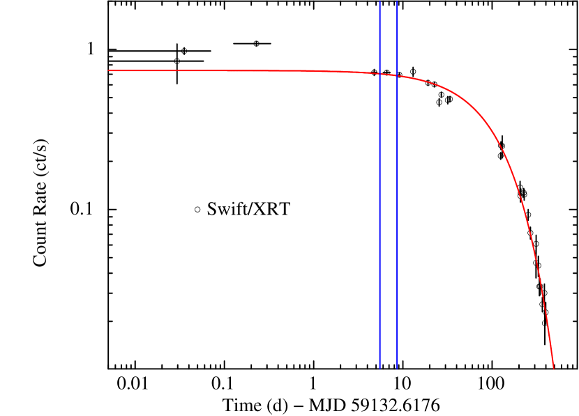
Figure 1: 0.5–10 keV Swift-XRT light curve of SGR J1830$-$0645 over a baseline of $\sim$ 400 d since the onset of the outburst (MJD 59132.6176). The red solid line denotes the best-fitting exponential function with an e-folding time of 113 $\pm$ 4 d. The vertical blue solid lines mark the observation span of the AstroSat observation.

Figure 1 shows the evolution of the 0.5–10 keV count rate of SGR J1830$-$0645 extracted from the 32 observations made with Swift-XRT (Evans et al., 2007) over a baseline of about 400 d starting from the onset of the outburst (MJD 59132.6176). The time evolution of the count rate can be described with an exponential function ($\propto e^{-t/\tau}$ – shown by the solid red line) with an e-folding time ($\tau$) of 113 $\pm$ 4 days ($\chi^{2}$ = 221 for 29 degrees of freedom, dof) which is nearly double that reported by Coti Zelati et al. (2021) using the first 34 d of data coverage of SGR J1830$-$0645.

3.1 Timing Analysis

Figure 2 shows the SXT (0.9–7 keV) and LAXPC (3–25 keV) light curves of SGR J1830$-$0645 binned with 2.3775 s and 0.1 s, respectively. Several short bursts lasting a few milliseconds were detected only with LAXPC during this observation.

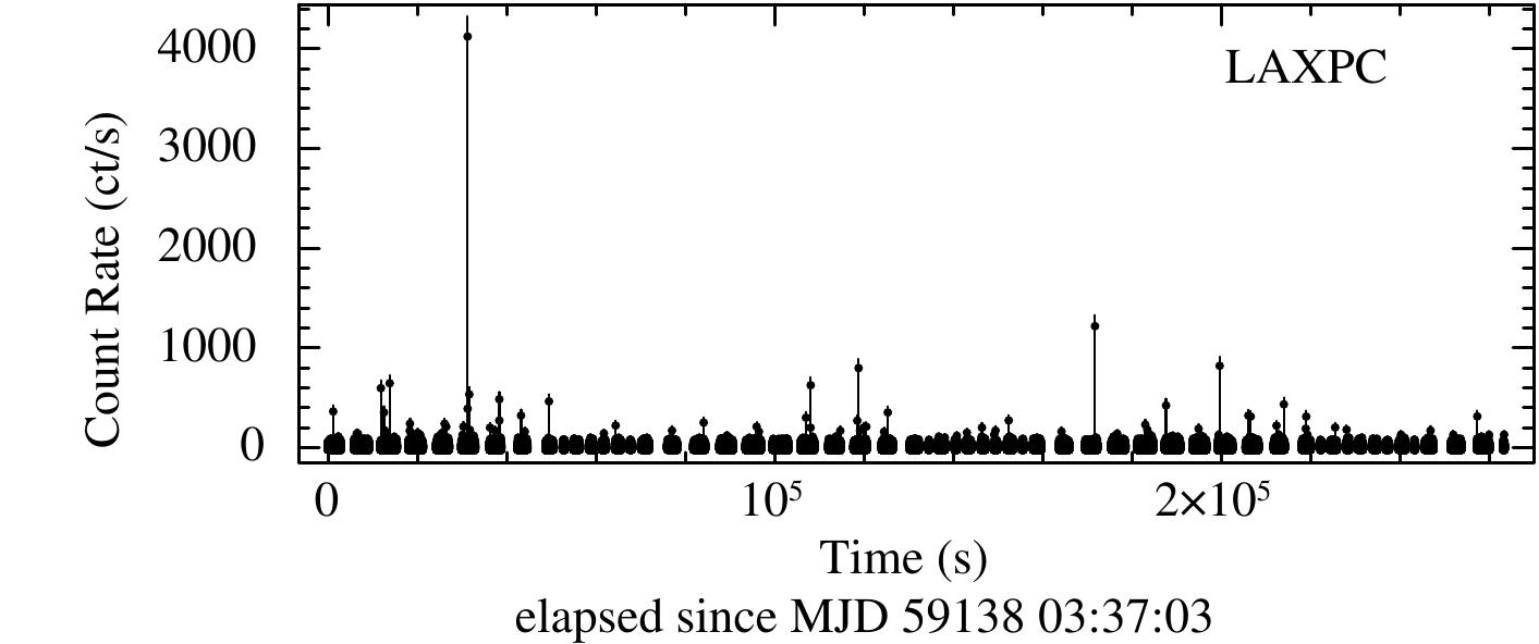
Figure 2: Top: The 0.9–7 keV AstroSat-SXT light curve of SGR J1830$-$0645 binned at 2.3775 s. Bottom: The 3–25 keV AstroSat-LAXPC light curve of SGR J1830$-$0645 binned at 0.1 s.

We used the $\chi^{2}$ maximization technique to determine the spin period of SGR J1830$-$0645. From the literature, the spin period is known to be $\sim$ 10.4157 s. We folded the LAXPC light curve over a range of periods (10.410 – 10.420 s) with a resolution of $10^{-6}$ s by using the efsearch tool of the XRONOS subpackage of FTOOLS (Blackburn et al., 1999). We obtained a spin period of 10.415730 s for epoch MJD 59138. We have detected pulsations only up to 10 keV. The error in the spin period was estimated by using the bootstrap method (Lutovinov et al., 2012; Boldin et al., 2013). We simulated 1000 light curves by the method described in Sharma et al. (2022); Sharma et al. (2023a) and obtained the spin period for each of them by using the epoch-folding technique. We obtained a standard deviation of $4\times 10^{-6}$ s in the best spin period distribution. This number was taken as the error of the pulse period. From SXT data, we found a spin period of 10.41572 (1) s, consistent with the estimate from the LAXPC data. Using a phase-coherent timing analysis, we have estimated the limit on the spin period derivative to be $\lvert\dot{P}\rvert<2\times 10^{-10}$ s s^-1 at a 90% confidence limit.

Figure  3 shows the energy-resolved pulse profiles of SGR J1830$-$0645, generated from SXT (in the energy ranges 0.9–3, 3–7, and 0.9–7 keV) and LAXPC (in the energy ranges 3–6, 6–10, and 3–10 keV), using the spin period derived with LAXPC. The SXT profiles show a phase shift of $\sim 1.4$ s relative to LAXPC, also observed in the pulse profiles reported by Beri et al. (2021). This phase shift could be instrumental and related to the readout time of the SXT CCD. The 0.9–3 keV SXT pulse profile displayed an asymmetric single-peak morphology with a minor peak just before the main peak. The 3–7 keV SXT profile was also asymmetric but relatively smoother. The pulsed fraction (defined as the semi-amplitude of the modulation in the pulse profile divided by the average source count rate) was found to increase from about 30% at 0.9–3 keV energy to 37% at 3–7 keV. The LAXPC pulse profile displayed a similar morphology, with a minor peak in the rising part of the profile at low energies (3–6 keV), which could possibly be attributed to hotspots on the neutron star surface while the profile in the 6–10 keV is more complex. Similar features were observed in the pulse profiles extracted from the XMM–Newton and NICER observations (Coti Zelati et al., 2021; Younes et al., 2022a). The LAXPC pulsed fraction was found to decrease from $\sim$34$\%$ (below 6 keV) to $\sim$20$\%$ (at 6–10 keV). Figure  4 shows the significant evolution of the pulsed fraction with energy in SGR J1830$-$0645. It increases up to energies around 5 keV and shows a steep drop thereafter, a behaviour also reported by Coti Zelati et al. (2021) and Younes et al. (2022b).

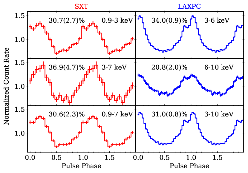
Figure 3: Energy-resolved pulse profile of SGR J1830$-$0645, generated from SXT (left panels) and LAXPC (right panels). The respective pulsed fraction values are noted in each panel. Two rotation cycles of the pulsar are shown for clarity.

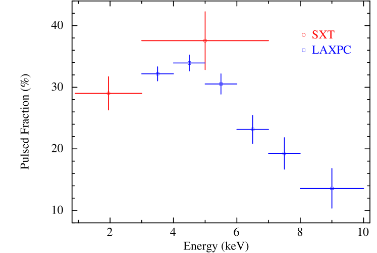
Figure 4: Evolution of the pulsed fraction in SGR J1830$-$0645 with energy as seen in the SXT and LAXPC data.

3.2 Spectral Analysis

We have performed a spectral analysis of the persistent-only emission of SGR J1830$-$0645. We simultaneously fitted spectra from SXT and LAXPC in the 0.9–25 keV energy range to study the spectral properties of the source. We have ignored LAXPC20 data above 25 keV because of the large uncertainty in the background estimation (Antia et al., 2017; Sharma et al., 2023a). We have used xspec v12.12.0 from the heasoft 6.29 package for spectral fitting (Arnaud, 1996). We used a systematic uncertainty of 1% during spectral fitting (Antia et al., 2017). The SXT and LAXPC spectra were grouped using grppha to have a minimum count of 50 counts per bin. A constant factor of 1 fixed for LAXPC was added for cross-calibration.

Figure 5 shows the 0.9–25 keV energy spectrum of SGR J1830$-$0645 which can be described with a model comprising a double blackbody along with a power-law component (bbodyrad+bbodyrad+powerlaw) (Coti Zelati et al., 2021). This model has a $\chi^{2}$ value of 323 for 253 dof. The addition of a Gaussian feature around 6.4 keV improved the fit ($\chi^{2}$/dof = 276/250) with an F-test probability of improvement by chance of about $10^{-8}$, which corresponds to $5.6\sigma$ significance. The parameters of the best-fitting spectral model are given in Table 2. They are consistent with those of Coti Zelati et al. (2021), except for the emission line.

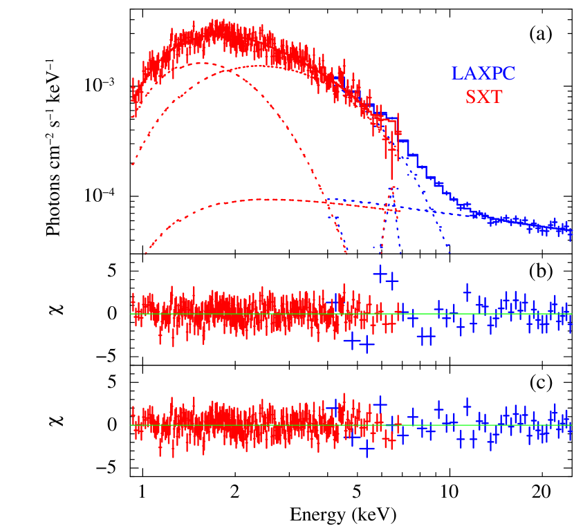
Figure 5: Panel (a): The 0.9–25 keV energy spectrum of SGR J1830$-$0645 obtained from SXT and LAXPC data. (b): The residuals for a model comprising continuum emission components without a Gaussian emission line. (c): The residuals with a best-fitting model comprising two blackbodies, a power-law and a Gaussian components.

Table 2: Best-fitting spectral parameters of SGR J1830$-$0645. All errors reported in this table are at a 90% confidence level ($\Delta\chi^{2}=2.7$).

Component	Parameter	Value
Tbabs	$N_{H}$ ($10^{22}$ cm-2)	$1.00^{+0.22}_{-0.19}$
Bbodyrad	$kT_{\rm Hot}$ (keV)	$1.096_{-0.04}^{+0.05}$
	$R_{\rm BB}$ (km)b	$0.65_{-0.07}^{+0.06}$
	norm	$2.66_{-0.56}^{+0.51}$
Bbodyrad	$kT_{\rm Warm}$ (keV)	$0.46_{-0.07}^{+0.09}$
	$R_{\rm BB}$ (km)b	$2.37_{-0.55}^{+1.25}$
	norm	$35.1_{-16.4}^{+37.0}$
Powerlaw	$\Gamma$	$0.39\pm 0.13$
	norm ($10^{-4}$)	$1.73_{-0.5}^{+0.8}$
Gaussian	$E_{\rm line}$ (keV)	$6.44\pm 0.15$
	Sigma (keV)	$0.26_{-0.24}^{+0.25}$
	norm ($10^{-5}$)	$9.7_{-2.6}^{+3.4}$
	EQW (keV)	$0.24^{+0.10}_{-0.09}$
Factor	$C_{\rm SXT}$	$0.91\pm 0.04$
	$F^{\rm BB-hot}_{0.9-25\rm~{}keV}$	$4.06\times 10^{-11}$
	$F^{\rm BB-warm}_{0.9-25\rm~{}keV}$	$1.40\times 10^{-11}$
Unabs. fluxa	$F^{\rm Powerlaw}_{0.9-25\rm~{}keV}$	$3.03\times 10^{-11}$
	$F^{\rm Total}_{0.9-25\rm~{}keV}$	$8.60\times 10^{-11}$
	$F^{\rm Total}_{0.1-100\rm~{}keV}$	$3.40\times 10^{-10}$
	$\chi^{2}/{\rm dof}$	276.6/250
$Note:$ aFlux is in units of erg cm-2 s-1.
bAssuming a fiducial distance of 4 kpc (Younes et al., 2022a).

The inclusion of an emission line component in the energy spectrum improved the best-fitting statistics by $\Delta\chi^{2}$ of 46.8 for 3 additional dof. Although popular amongst the astrophysics community, the F-test is associated with caveats when it comes to the detection of emission lines in a spectral model (Protassov et al., 2002). Therefore, we estimated the significance of the potential spectral line by using the simftest script from xspec. This routine uses the Monte Carlo method to simulate data sets with the same counting statistics as the original data. We simulated 10,000 data sets, which were fitted with the best-fitting spectral models (both with and without a 6.4 keV emission line). Figure 6 shows the distribution of $\Delta\chi^{2}$ values obtained from fitting every simulated data set. From the simftest routine, we obtained a maximum $\Delta\chi^{2}$ of 15, which is significantly lower than the $\Delta\chi^{2}$ of 46.8 obtained in the original data. A large deviation of $\Delta\chi^{2}$ confirms a significant detection of the emission line in the spectra. To be doubly sure, we also tested whether the presence of spectral line is due to systematics in the LAXPC instrument. For this, we increased the systematic error in the spectral fitting to 2%. We found an improvement of $\Delta\chi^{2}$ of 20 for 3 additional dof; the F-test probability of finding such a change by chance is $\sim 3\times 10^{-4}$, which corresponds to $3.6\sigma$ significance. It is important to mention here that the spectral analysis of observations made with the X-ray missions XMM–Newton and NuSTAR has not detected the presence of this spectral line (Coti Zelati et al., 2021). Even a dedicated NICER monitoring of the source has not shown any evidence of the presence of emission lines (Younes et al., 2022a). Therefore, even though we have performed thorough statistical checks that support the presence of the emission line, it is possible that the 6.4 keV feature observed in our data is an instrumental effect. If our detection of line emission in the persistent emission of SGR J1830$-$0645 is indeed true, then it has several implications for the X-ray emission mechanism of magnetars, some of which are highlighted in Section 4.

In order to check the correlation between the emission line and burst/non-burst phase of SGR J1830$-$0645, we generated stacked spectra from 100, 200, 300, 400, and 500 s data before and after each burst. The spectrum from all the segments showed the presence of a $\sim$6.4 keV emission line with a probability of chance improvement $<10^{-4}$ (i.e. significance $>3\sigma$) using simftest, except for the first 100 s segment where we obtained a probability of 0.0029. A relatively high probability, in this case, could be due to overall low exposure ($\sim$ 6.2 ks compared to more than 20 ks for other segments) and thus poorer statistics. The equivalent width of the emission line during these segments was similar to that obtained in the average spectrum of the source ($\sim$0.25–0.30 keV), clearly indicating that the presence of line is not related to the occurrence of bursts in SGR J1830$-$0645.

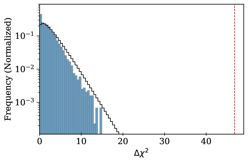
Figure 6: Histogram showing the results of the simftest simulations for testing the detection significance of the emission line. The overlaid solid black curve represents the $\chi^{2}$ distribution for 3 dof. The vertical red dashed line marks the $\Delta\chi^{2}$ obtained from spectral fitting of the real data.

3.3 Burst Analysis

In order to quantify the occurrence of X-ray bursts, we used only the LAXPC data because of the relatively large time resolution (2.37 s) of SXT. We binned the 3–25 keV LAXPC time series with a time resolution of 0.01 s. We searched for bursts in every Good Time Interval (GTI) of the time series by using the find_peaks routine of the scipy package (Virtanen et al., 2020).

Using a Poisson distribution, the probability ($P_{i}$) of the number of counts occurring randomly in each time bin ($n_{i}$) is given by,

$$P_{i}=\frac{\lambda^{n_{i}}e^{-\lambda}}{n_{i}!}$$ (1)

Here, $\lambda$ is the local mean count rate of every GTI. The events for which $P_{i}$ was less than 10${}^{-4}/N$, were labelled as bursts. Here, $N$ is the total number of time bins in the respective GTI (Gavriil et al., 2004; Borghese et al., 2020). Using this algorithm, we have detected a total of 67 bursts. Figure 7 shows the profile of the two brightest bursts observed with LAXPC. The brightest burst had a peak count of about 100 counts in a 10 ms bin, corresponding to a fluence of about 419 counts within a duration of 0.09 s.

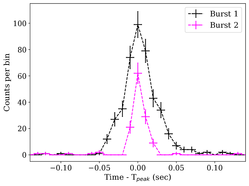
Figure 7: The 3–25 keV profile of the two brightest bursts observed with LAXPC.

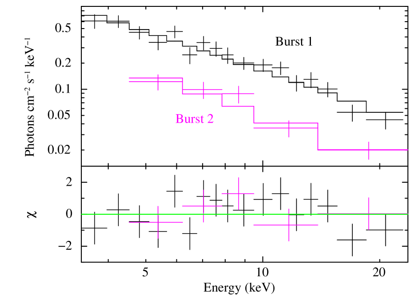
Figure 8: The spectra of the two brightest bursts detected during the AstroSat observation of SGR J1830$-$0645. The bottom panel shows the residuals with respect to the best-fitting absorbed power-law model.

Figure 8 shows the 3–25 keV burst spectra that have been modelled with an absorbed power-law ($\chi^{2}/$dof=17.9/18) with $\Gamma=1.52\pm 0.14$ where $N_{H}$ was fixed at $1.0\times 10^{22}$ cm^-2 (Table 3). For both the bursts, the LAXPC energy spectra could not be modelled with a single blackbody as reported in the literature (Coti Zelati et al., 2021; Younes et al., 2022a). For the brightest burst, we obtained an unabsorbed 3–25 keV flux of $5.41\times 10^{-8}$ erg cm^-2 s^-1, corresponding to a fluence of $\sim 5\times 10^{-9}$ erg  cm^-2. To date, the Swift-BAT burst detected on 2020 November 5 has the highest reported fluence ($\sim 3.2\times 10^{-8}$ erg  cm^-2) in 15–150 keV (Coti Zelati et al., 2021). On extrapolating our results, we obtained a 15–150 keV fluence of $\sim 1.1\times 10^{-8}$ erg  cm^-2. The cumulative spectrum of all the 67 bursts is also well described with a power-law ($\Gamma\sim 1.7$) model having an average 3–25 keV unabsorbed flux of $\sim$1$\times$10^-10 erg cm^-2 s^-1. The burst spectra did not show any evidence of the presence of the $\sim$6.4 keV emission line.

The left panel of Figure 9 shows the fluence distribution of all 67 bursts. The 3–25 keV high-fluence tail in this distribution ranges from $(0.2-48)\times 10^{-10}$ erg cm^-2. This tail can be described by a power-law function having an index of $\sim$1.88. From the 0.7-8 keV NICER data, Younes et al. (2022a) described the high-fluence tail with a power-law function having an index of 1.5. The right panel of Figure 9 shows the distribution of the burst duration ($T_{90}$). The average duration of all 67 bursts was about 33 ms with a standard deviation of 13 ms.

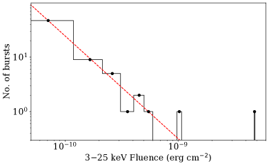
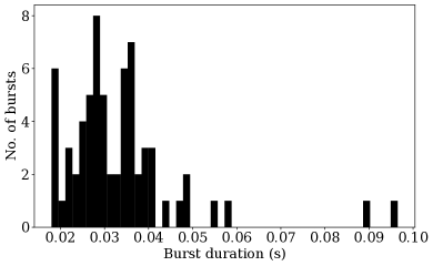
Figure 9: Left: The fluence distribution of 3–25 keV bursts detected with AstroSat in SGR J1830$-$0645. The red dashed line shows the best-fitting power-law trend ($F^{-1.88}$). Right: Distribution of the duration ($T_{90}$) of the X-ray bursts.

Table 3: Spectral parameters of the two brightest bursts detected in SGR J1830$-$0645 with LAXPC. The best-fitting model used was the absorbed power-law.

Component	Parameter	Burst 1	Burst 2
Tbabs	$N_{H}$ ($10^{22}$ cm-2)	$1.0^{\rm fixed}$
Powerlaw	$\Gamma$	$1.52\pm 0.14$	$1.56\pm 0.38$
	norm	$5.4_{-1.4}^{+1.9}$	$1.9_{-1.1}^{+2.4}$
Unabs. Flux	$F_{3-25\rm keV}$ (erg cm-2 s-1)	$5.41\times 10^{-8}$	$1.69\times 10^{-8}$
Unabs. Flux	$F_{0.1-100\rm keV}$ (erg cm-2 s-1)	$1.58\times 10^{-7}$	$4.87\times 10^{-8}$
	$\chi^{2}/{\rm dof}$	17.9/18

4 DISCUSSION

This work reports results from the timing and spectral analyses of the AstroSat observation of SGR J1830$-$0645 made on 2020 October 16 during its first detected outburst. We conclude the following from our findings.

1. Detection of 0.9–10 keV pulsations in SGR J1830$-$0645.

2. Pulse period of 10.415730 (4) s at an epoch of MJD 59138.

3. Variation in the morphology of the pulse profiles with energy (pronounced dip just before the main peak at low energies and almost sinusoidal at higher energies) along with significant variation in the pulsed fraction.

4. The 0.9–25 keV SXT+LAXPC energy spectrum comprising the sum of two thermal components and a power-law component.

5. Tentative detection of a 6.4 keV emission line with an equivalent width of about 0.24 keV.

6. Detection of several short subsecond X-ray bursts during this observation of AstroSat.

The pulsed fraction of SGR J1830$-$0645 shows a significant evolution with increasing energy. It is observed to increase for energies up to $\sim$5 keV and shows a steep drop thereafter. This trend is different from that observed in several other magnetars, such as 1E 1841-045, 1E 2259+586, and 4U 0142+61 (Kuiper et al., 2006; An et al., 2013; Vogel et al., 2014). Clearly, the pulsed fraction trend seen in SGR J1830$-$0645 is in stark contrast to the coronal outflow model of Beloborodov (2013).

SGR J1830$-$0645 displays spectral properties typical of most magnetars in the soft X-ray band (Thompson et al., 2002; Tiengo et al., 2008; Coti Zelati et al., 2018). The energy spectrum consists of two blackbody (thermal) components along with non-thermal power-law associated with resonantly up-scattered soft thermal photons as they traverse from the stellar surface through the magnetosphere (Fernández & Thompson, 2007; Nobili et al., 2008; Coti Zelati et al., 2021). Assuming a distance of 4 kpc (Younes et al., 2022a), we have estimated the size of the emitting regions to be $R_{\rm BB}$ of 0.65 km (for $kT_{\rm BB}$ of 1.1 keV) and $R_{\rm BB}$ of 2.45 km ($kT_{\rm BB}$ of 0.46 keV). During this observation, the blackbody components carried about 47% (hot component) and 16% (warmer component) fractions of the total flux.

We detected a total of 67 bursts from the LAXPC data set with an average duration of 33 ms. The brightest burst lasted for $\sim$90 ms and had a fluence of $\sim 5\times 10^{-9}$ erg  cm^-2 in the 3–25 keV energy range. The fluence tail of the bursts can be described by a power-law function of index $\sim$1.88. The power-law fluence distribution of burst fluence observed in SGR J1830$-$0645 is similar to several magnetars (see e.g., Cheng et al., 1996; Scholz & Kaspi, 2011; Collazzi et al., 2015) and is believed to be consistent with either magnetospheric reconnection or the crust-quake theories of the burst-triggering mechanism (for example, see Thompson & Duncan, 1995; Lyutikov, 2003).

We have detected the presence of an emission line-like feature in SGR J1830$-$0645. This detection makes SGR J1830$-$0645 one of the few magnetars that have shown the presence of emission lines. In the case of SGR 1900+14, an emission feature at 6.4 keV accompanied by a faint hint of its harmonic at $\sim$13 keV was detected during the first 0.3 s of the precursor of a strong burst (Strohmayer & Ibrahim, 2000). In XTE J1810–197, a narrow 12.6 keV emission feature was reported by Woods et al. (2005) by using RXTE data during the bright X-ray tail of a burst. In 1E 1048.1–5937, Gavriil et al. (2002) reported the presence of a $\sim$14 keV emission feature during the initial stages of a burst detected with RXTE. For this magnetar, An et al. (2014) also reported a $\sim$13 keV emission feature using NuSTAR data, thereby ruling out any instrumental effects. In all these magnetars, the emission line is a transient feature observed occasionally during the burst, but we have found the emission feature during persistent emission in SGR J1830$-$0645. We did not find evidence for this emission line in the individual spectra of the two brightest bursts nor in the cumulative burst spectra.

There are several possibilities that could explain the presence of this emission line but, owing to the lack of sufficient data, these possibilities come with many limitations. It is possible that the emission line is a result of the fluorescence of iron due to the presence of relatively cool material near the neutron star. We have detected an emission line with an equivalent width of about $\sim 0.24$ keV. This is similar to the emission line generally observed in accreting X-ray pulsars (e.g., Naik et al., 2011; Naik & Paul, 2012; Sharma et al., 2023a). Another possibility for the presence of the emission line is related to proton and alpha-particle cyclotron transitions in astrophysical systems with ultrastrong magnetic fields (Strohmayer & Ibrahim, 2000; Ibrahim et al., 2002; Ibrahim et al., 2007). For magnetars having $B\lesssim 10^{14}$ G, the electron cyclotron absorption line energy is $\mathcal{O}$(MeV), which is out of bounds for AstroSat detectors. The proton and alpha-particle cyclotron resonances are well within reach, with fundamentals at $E_{p}=6.3(1+z)^{-1}(B/10^{15}G)$ keV and $E_{\alpha}=3.2(1+z)^{-1}(B/10^{15}G)$ keV, respectively. Using $(1+z)=1.31$ for canonical neutron star of $M=1.4M_{\sun}$ and $R=10$ km, the surface field strength in SGR J1830$-$0645 comes out to be $\sim 1.3\times 10^{15}$ G for proton cyclotron resonances which is slightly higher than the dipole magnetic field strength derived from the spin-down measurements by Younes et al. (2022a) and Coti Zelati et al. (2021).

In spite of these possibilities and owing to the fact that the emission line has not been detected with other X-ray missions (Coti Zelati et al., 2021; Younes et al., 2022a), it is possible that its presence in the AstroSat observation is an instrumental systematic effect. Thus, more data and intensive analysis are required before commenting on its viability.

Data Availability

Data used in this work can be accessed through the Indian Space Science Data Center (ISSDC) at https://astrobrowse.issdc.gov.in/astro_archive/archive/Home.jsp.

References

- Agrawal (2006) Agrawal P. C., 2006, Advances in Space Research, 38, 2989
- Agrawal et al. (2017) Agrawal P. C., et al., 2017, Journal of Astrophysics and Astronomy, 38, 30
- An et al. (2013) An H., et al., 2013, ApJ, 779, 163
- An et al. (2014) An H., et al., 2014, ApJ, 790, 60
- Antia et al. (2017) Antia H. M., et al., 2017, ApJS, 231, 10
- Antia et al. (2021) Antia H. M., et al., 2021, Journal of Astrophysics and Astronomy, 42, 32
- Arnaud (1996) Arnaud K. A., 1996, in Jacoby G. H., Barnes J., eds, Astronomical Society of the Pacific Conference Series Vol. 101, Astronomical Data Analysis Software and Systems V. p. 17
- Astropy Collaboration et al. (2018) Astropy Collaboration et al., 2018, AJ, 156, 123
- Beloborodov (2013) Beloborodov A. M., 2013, ApJ, 762, 13
- Beri et al. (2021) Beri A., et al., 2021, MNRAS, 500, 565
- Blackburn et al. (1999) Blackburn J. K., Shaw R. A., Payne H. E., Hayes J. J. E., Heasarc 1999, FTOOLS: A general package of software to manipulate FITS files, Astrophysics Source Code Library, record ascl:9912.002 (ascl:9912.002)
- Boldin et al. (2013) Boldin P. A., Tsygankov S. S., Lutovinov A. A., 2013, Astronomy Letters, 39, 375
- Borghese et al. (2020) Borghese A., Coti Zelati F., Rea N., Esposito P., Israel G. L., Mereghetti S., Tiengo A., 2020, ApJ, 902, L2
- Cheng et al. (1996) Cheng B., Epstein R. I., Guyer R. A., Young A. C., 1996, Nature, 382, 518
- Collazzi et al. (2015) Collazzi A. C., et al., 2015, ApJS, 218, 11
- Coti Zelati et al. (2018) Coti Zelati F., Rea N., Pons J. A., Campana S., Esposito P., 2018, MNRAS, 474, 961
- Coti Zelati et al. (2021) Coti Zelati F., et al., 2021, ApJ, 907, L34
- Duncan & Thompson (1992) Duncan R. C., Thompson C., 1992, ApJ, 392, L9
- Evans et al. (2007) Evans P. A., et al., 2007, A&A, 469, 379
- Fernández & Thompson (2007) Fernández R., Thompson C., 2007, ApJ, 660, 615
- Gavriil et al. (2002) Gavriil F. P., Kaspi V. M., Woods P. M., 2002, Nature, 419, 142
- Gavriil et al. (2004) Gavriil F. P., Kaspi V. M., Woods P. M., 2004, ApJ, 607, 959
- Gogus et al. (2020a) Gogus E., Kouveliotou C., Younes G., 2020a, The Astronomer’s Telegram, 14085, 1
- Gogus et al. (2020b) Gogus E., Kouveliotou C., Younes G., 2020b, The Astronomer’s Telegram, 14097, 1
- Harris et al. (2020) Harris C. R., et al., 2020, Nature, 585, 357
- Hunter (2007) Hunter J. D., 2007, Computing in Science and Engineering, 9, 90
- Ibrahim et al. (2002) Ibrahim A. I., Safi-Harb S., Swank J. H., Parke W., Zane S., Turolla R., 2002, ApJ, 574, L51
- Ibrahim et al. (2007) Ibrahim A. I., et al., 2007, Ap&SS, 308, 535
- Kaspi & Beloborodov (2017) Kaspi V. M., Beloborodov A. M., 2017, ARA&A, 55, 261
- Kuiper et al. (2006) Kuiper L., Hermsen W., den Hartog P. R., Collmar W., 2006, ApJ, 645, 556
- Lutovinov et al. (2012) Lutovinov A., Tsygankov S., Chernyakova M., 2012, MNRAS, 423, 1978
- Lyutikov (2003) Lyutikov M., 2003, MNRAS, 346, 540
- Naik & Paul (2012) Naik S., Paul B., 2012, Bulletin of the Astronomical Society of India, 40, 503
- Naik et al. (2011) Naik S., Paul B., Ali Z., 2011, ApJ, 737, 79
- Nobili et al. (2008) Nobili L., Turolla R., Zane S., 2008, MNRAS, 386, 1527
- Olausen & Kaspi (2014) Olausen S. A., Kaspi V. M., 2014, ApJS, 212, 6
- Page et al. (2020) Page K. L., Barthelmy S. D., Klingler N. J., Kuin N. P. M., Lien A. Y., 2020, The Astronomer’s Telegram, 14083, 1
- Protassov et al. (2002) Protassov R., van Dyk D. A., Connors A., Kashyap V. L., Siemiginowska A., 2002, ApJ, 571, 545
- Ramadevi et al. (2018) Ramadevi M. C., et al., 2018, Journal of Astrophysics and Astronomy, 39, 11
- Rao et al. (2017) Rao A. R., Bhattacharya D., Bhalerao V. B., Vadawale S. V., Sreekumar S., 2017, Current Science, 113, 595
- Ray et al. (2020) Ray P. S., et al., 2020, The Astronomer’s Telegram, 14112, 1
- Rea & Esposito (2011) Rea N., Esposito P., 2011, in High-Energy Emission from Pulsars and their Systems. p. 247 (arXiv:1101.4472), doi:10.1007/978-3-642-17251-9_21
- Rodríguez Castillo et al. (2016) Rodríguez Castillo G. A., et al., 2016, MNRAS, 456, 4145
- Scholz & Kaspi (2011) Scholz P., Kaspi V. M., 2011, ApJ, 739, 94
- Sharma et al. (2020) Sharma R., Beri A., Sanna A., Dutta A., 2020, MNRAS, 492, 4361
- Sharma et al. (2022) Sharma P., Jain C., Dutta A., 2022, MNRAS, 513, L94
- Sharma et al. (2023a) Sharma R., Jain C., Rikame K., Paul B., 2023a, MNRAS, 519, 1764
- Sharma et al. (2023b) Sharma R., Sanna A., Beri A., 2023b, MNRAS, 519, 3811
- Singh et al. (2014) Singh K. P., et al., 2014, in Space Telescopes and Instrumentation 2014: Ultraviolet to Gamma Ray. p. 91441S, doi:10.1117/12.2062667
- Singh et al. (2016) Singh K. P., et al., 2016, in den Herder J.-W. A., Takahashi T., Bautz M., eds, Society of Photo-Optical Instrumentation Engineers (SPIE) Conference Series Vol. 9905, Space Telescopes and Instrumentation 2016: Ultraviolet to Gamma Ray. p. 99051E, doi:10.1117/12.2235309
- Singh et al. (2017) Singh K. P., et al., 2017, Journal of Astrophysics and Astronomy, 38, 29
- Strohmayer & Ibrahim (2000) Strohmayer T. E., Ibrahim A. I., 2000, ApJ, 537, L111
- Tandon et al. (2017) Tandon S. N., et al., 2017, AJ, 154, 128
- Thompson & Duncan (1995) Thompson C., Duncan R. C., 1995, MNRAS, 275, 255
- Thompson & Duncan (1996) Thompson C., Duncan R. C., 1996, ApJ, 473, 322
- Thompson et al. (2002) Thompson C., Lyutikov M., Kulkarni S. R., 2002, ApJ, 574, 332
- Tiengo et al. (2008) Tiengo A., Esposito P., Mereghetti S., 2008, ApJ, 680, L133
- Tiengo et al. (2013) Tiengo A., et al., 2013, Nature, 500, 312
- Virtanen et al. (2020) Virtanen P., et al., 2020, Nature Methods, 17, 261
- Vogel et al. (2014) Vogel J. K., et al., 2014, ApJ, 789, 75
- Woods et al. (2005) Woods P. M., et al., 2005, ApJ, 629, 985
- Yadav et al. (2016) Yadav J. S., et al., 2016, in Space Telescopes and Instrumentation 2016: Ultraviolet to Gamma Ray. p. 99051D, doi:10.1117/12.2231857
- Younes et al. (2020) Younes G., et al., 2020, The Astronomer’s Telegram, 14086, 1
- Younes et al. (2022a) Younes G., et al., 2022a, ApJ, 924, 136
- Younes et al. (2022b) Younes G., et al., 2022b, ApJ, 924, L27
- den Hartog et al. (2008a) den Hartog P. R., Kuiper L., Hermsen W., Kaspi V. M., Dib R., Knödlseder J., Gavriil F. P., 2008a, A&A, 489, 245
- den Hartog et al. (2008b) den Hartog P. R., Kuiper L., Hermsen W., 2008b, A&A, 489, 263