Neutrino CP Measurement in the Presence of RG Running with Mismatched Momentum Transfers

Abstract

The neutrino mixing parameters are expected to have RG running effect in the presence of new physics. If the momentum transfers at production and detection mismatch with each other, the oscillation probabilities are generally modified and become dependent on not just the neutrino energy but also the momentum transfer. Even in the limit of vanishing baseline, the transition probability for the appearance channel is interestingly not zero. This would significantly affect the sensitivity of the genuine leptonic Dirac CP phase. We further explore the possibility of combing the long- and short-baseline neutrino experiments to constrain such RG running effect for the purpose of guaranteeing the CP measurement. To simulate the double dependence on the neutrino energy and momentum transfer, we extend the usual GLoBES simulation of fixed baseline experiments and use a two-dimensional $\chi^{2}$ analysis to obtain sensitivities.

1 Introduction

The matter-antimatter asymmetry in the Universe is one of the most fundamental questions [1]. To explain this asymmetry, the charge-parity (CP) violation is necessary [2]. In the Standard Model (SM) of particle physics, the quark mixing matrix introduces a CP phase but the induced baryon asymmetry is too small to account for the observed value [3, 4, 5]. In the extended SM with heavy right-handed neutrinos, it has been shown that the leptonic CP violation could generate sufficient matter–antimatter disparity through the leptogenesis mechanism [6, 7, 8]. It is interesting to observe that the leptonic CP phases in the neutrino mixing matrix [9] provide potential sources of CP violation that can be directly used to explain the matter-antimatter asymmetry [10, 11, 12, 13, 14, 15, 16].

The leptonic Dirac CP phase $\delta_{D}$ of the PMNS matrix can manifest itself in neutrino oscillation and hence can be measured therein. Its first measurement results were published in 2019 [17, 18] by the two long-baseline (LBL) neutrino oscillation experiments NO$\nu$A [19] and T2K [20]. With the normal ordering (NO) of neutrino masses that is preferred by the latest results, the 2021 NO$\nu$A result gives $\delta_{D}=148^{\circ}{}^{+49^{\circ}}_{-157^{\circ}}$ [21] while the 2023 T2K result has $\delta_{D}=247^{\circ}{}^{+56^{\circ}}_{-36^{\circ}}$ [22]. The next-generation LBL experiments T2HK [24] and DUNE [23] under construction are expected to greatly improve the precision on $\delta_{D}$. With about 10 years of data taking, each experiment can reach $\sim 10^{\circ}$ precision level [25, 26]. In addition, ESS$\nu$SB [27] is sensitive to $\delta_{D}$ by detecting neutrinos at the second oscillation peak, while T2HKK [28] and MOMENT [29] are sensitive to both the first and second oscillation maxima. With around twice the energy and baseline of DUNE, the P2O experiment [30] is sensitive to both $\delta_{D}$ and the matter effect. Additional low-energy neutrinos from muon decay at rest ($\mu$DAR) provide complementary measurements to accelerator LBL experiments, such as DAE$\delta$ALUS [31], TNT2HK [34], $\mu$DARTS [32, 33], DAE$\delta$ALUS+JUNO [35], and DUNE+$\mu$THEIA [36]. Besides accelerator neutrinos, CP measurement with sub-GeV atmospheric neutrino oscillation is also proposed for Super-PINGU [37, 38], Super-ORCA [39], and even at JUNO [40] or DUNE [41].

Although the neutrino oscillation measurement has entered the precision era [42, 43], the interpretation of the experimental data to extract the leptonic Dirac CP phase $\delta_{D}$ still faces various theoretical challenges. On the SM side, the matter density uncertainty can greatly reduce the sensitivity to $\delta_{D}$, especially when the value of $\delta_{D}$ is around the maximal values $90^{\circ}$ or $270^{\circ}$ [44, 45, 46, 47, 36]. Beyond the SM, there are various new physics scenarios that are capable of mimicking the CP violation effect and hence disturbing the CP measurement. For example, the neutrino non-standard interaction (NSI) contributes extra matter potential [48, 49] that receives different sign between neutrino and anti-neutrino modes to fake CP and significantly reduce the CP phase sensitivity [50, 51, 52, 53, 54, 55]. In addition, the Lorentz invariance violation (LIV) [56, 57] induces an effective Hamiltonian with both CPT-odd and CPT-even terms that have similar form as the effective Hamiltonian induced by NSI. Consequently, the effective Hamiltonian will modify the neutrino oscillation probability and hence impact on the CP phase sensitivity just like NSI [59, 60, 58, 61]. Moreover, the non-unitary mixing due to heavy neutrinos [62, 63] allows extra CP phases to fake the genuine CP effect [64, 51, 65, 66, 67, 68].

Besides the new physics scenarios listed above, both the SM and the BSM interactions can generate less explored effects in neutrino oscillation such as the renormalization group (RG) running of the neutrino mixing parameters [69, 70, 71, 72, 73, 74]. Various neutrino mass models, such as the canonical seesaw models, the inverse seesaw model, the scotogenic model, and the radiative Dirac model can lead to RG running effects [73, 74]. Consequently, the neutrino mass and mixing parameters evolve as functions of the relevant energy scale. With mismatched energy scales between the neutrino production and detection processes, the neutrino RG running can affect its oscillation probabilities [75].

In our paper, we carefully study how RG running can affect the leptonic CP phase measurement. In Sec. 2, we review the neutrino RG running features and introduce a model-independent parametrization for the running behaviors. We then establish in Sec. 3 the general formalism of neutrino oscillations in the presence of RG running. In particular, we adopt the quantum field theory (QFT) language and compare with the usually adopted quantum mechanics (QM) approach. With higher energy, DUNE can provide larger variation at the relevant energy scale than other experiments to allow more significant RG effects. In Sec. 4, we elaborate how a two-dimensional neutrino oscillation simulation, including neutrino energy and momentum transfer reconstructions, should be established for GLoBES with DUNE as a specific realization. The interplay between RG running and the genuine Dirac CP phase is evaluated with the extended two-dimensional $\chi^{2}$ analysis to give the projected sensitivities at DUNE. Our conclusion and discussion about this new effect can be found in Sec. 6.

2 RG Running of Neutrino Mixing Parameters

Although neutrino oscillation is the first new physics supported by various experimental measurements, we are still not so sure what is really happening behind the scene. The new physics that we have been looking for may not be as appearant as the non-standard interactions (NSI) that appears at tree level already and affects the neutrino oscillation behavior, but make itself manifest via loop correction and the RG running effect. Studying the RG running effect in neutrino oscillation is actually an inevitable way of exploring new physics.

The neutrino mixing matrix $U$ is defined according to the neutrino mass matrix diagonalization, $U^{\dagger}M^{\dagger}_{\nu}M_{\nu}U={\rm Diag}(m^{2}_{1},m^{2}_{2},m^{2}_{3})$. In other words, the RG running effect of the neutrino mixing is inherited from the running of the neutrino mass matrix. On the model building side, the neutrino mass is typically generated at a high scale while the mass value and the corresponding neutrino mixing parameters are measured experimentally at a low scale. Across different energy scales, the RG evolution effects need to be included.

The RG running of neutrino mixing can be generally parameterized using the $\beta$ function,

$$\frac{d\mathcal{O}_{\nu}}{d\ln|Q^{2}|}\equiv\beta_{\nu},$$ (2.1)

where the absolute value of momentum transfer $|Q^{2}|$ is taken as the evolution variable [75]. For generality, we use $\mathcal{O}_{\nu}$ to denote the neutrino observables such as the mixing angles and the Dirac CP phase. Below the new physics scale, the RG evolution determined by the SM [77, 76] is negligibly small [74] and hence the mixing parameters are treated as constants. Any sizable RG running effect should appear above the new physics scale. The neutrino masses can also run in a similar way as Eq. (2.1). However, the impact of running neutrino masses is negligible [70, 71, 72, 73, 74, 75] for the oscillation process of interest and hence omitted in this paper for simplicity.

For generality, we simply treat $\beta_{\nu}$ as a perturbative constant. In this sense, the solution of Eq. (2.1) for the three mixing angles ($\theta_{s}\equiv\theta_{12}$, $\theta_{a}\equiv\theta_{23}$, and $\theta_{r}\equiv\theta_{13}$) and the Dirac CP phase $\delta_{D}$ can be generally expressed as,

$$\theta_{ij}(Q^{2})\equiv\theta_{ij}(Q^{2}_{0})+\beta_{ij}\ln\left(\left|\frac{Q^{2}}{Q^{2}_{0}}\right|\right),\quad\mbox{and}\quad\delta_{D}(Q^{2})\equiv\delta_{D}(Q^{2}_{0})+\beta_{\delta}\ln\left(\left|\frac{Q^{2}}{Q^{2}_{0}}\right|\right).$$ (2.2)

The reference value $|Q^{2}_{0}|$ corresponds to the new physics scale and the evolution formulas apply for $|Q^{2}|>|Q^{2}_{0}|$ while reducing to constant values for $|Q^{2}|<|Q^{2}_{0}|$. If the new physics scale is much higher than the experimental scales, the running effect will not be measured at the current low energy neutrino experiments. To test the running effect at the $\mathcal{O}({\rm GeV})$ LBL experiments such as DUNE, we take $Q^{2}_{0}=1$ MeV as a benchmark value throughout this paper. Furthermore, we need four parameters to describe the evolution, three $\beta_{ij}$ for the mixing angles and one $\beta_{\delta}$ for the Dirac CP phase. The RG running effect can lead to non-standard oscillation behaviors as we elaborate below.

3 General Formalism of Neutrino Oscillation

3.1 QFT Description of Neutrino Oscillation

We start with the vacuum neutrino oscillation without considering RG running which is conceptually clearer to set the stage in the QFT framework. A typical neutrino oscillation experiment involves the neutrino production, propagation, and detection processes. For the case of neutrino (rather than anti-neutrino) oscillation, a charged anti-lepton $\bar{\ell}_{\alpha}$ appears at the position $x\equiv(x_{0},{\boldsymbol{x}})$ when producing an $\alpha$-flavor neutrino $\nu_{\alpha}$ while a charged lepton $\ell_{\beta}$ is observed at the position $y\equiv(y_{0},{\boldsymbol{y}})$ for the detection of a $\beta$-flavor neutrino $\nu_{\beta}$ as shown in Fig. 1. In between, neutrinos propagate as mass eigen-fields ($\nu_{i}\equiv\sum_{\alpha}U^{\ast}_{\alpha i}\nu_{\alpha}$) over a macroscopic spatial distance ${\boldsymbol{L}}\equiv{\boldsymbol{y}}-{\boldsymbol{x}}$. The full transition matrix element $\mathcal{T}$ for the above processes can be read off directly from Fig. 1 [78],

$$\mathcal{T}\equiv\sum_{i}\int d^{4}xd^{4}y\mathcal{M}^{\mu}_{\rm det}(y)\frac{ig}{\sqrt{2}}U_{\beta i}\bar{u}_{\beta}\gamma_{\mu}P_{L}\int\frac{d^{4}p}{(2\pi)^{4}}\frac{i(\not{p}+m_{i})e^{ip\cdot(x-y)}}{p^{2}-m^{2}_{i}+i\epsilon}\frac{ig}{\sqrt{2}}U^{*}_{\alpha i}\gamma_{\nu}P_{L}v_{\alpha}\mathcal{M}^{\nu}_{\rm prod}(x),\quad$$ (3.1)

where the production and detection matrix elements $\mathcal{M}^{\mu}_{\rm prod}(x)$ and $\mathcal{M}^{\nu}_{\rm det}(y)$ contain those relevant interactions except the charged-current vertex between neutrino and charged lepton. To also take the associated charged leptons into consideration, the charged current (CC) interaction mediated by the SM $W^{\pm}$ boson with weak gauge coupling $g$ should be involved. With $\overline{\psi}$ to produce a neutrino, the associated matrix element $U^{*}_{\alpha i}$ receives a complex conjugation. Similarly, the detection part annihilates the intermediate neutrino with $\psi$ to have $U_{\beta i}$. The projector $P_{L}$ selects the left-handed fermions.

The oscillation behavior as a periodic function of the baseline $L$ is encoded in the propagation phase factor $e^{ip\cdot(x-y)}$ from $x$ to $y$. For the mass eigenstate $\nu_{i}$ propagator,

$$\int\frac{d^{4}p}{(2\pi)^{4}}\frac{i(\not{p}+m_{i})e^{ip\cdot(x-y)}}{p^{2}-m^{2}_{i}+i\epsilon}=\int\frac{d^{4}p}{(2\pi)^{4}}\frac{i\sum_{s}u_{i}(p,s)\bar{u}_{i}(p,s)e^{ip\cdot(x-y)}}{p^{2}-m^{2}_{i}+i\epsilon},$$ (3.2)

its numerator can be replaced by two neutrino spinors according to the spin sum relation, $\not{p}+m_{i}=\sum_{s}u_{i}(p,s)\bar{u}_{i}(p,s)$. In the ultra-relativistic limit, only the left-handed chiral component can contribute since the right-handed counterpart is projected out by $P_{L}u(p,+)=0$. Then the neutrino spinors $u_{i}(p,-)\bar{u}_{i}(p,-)$ in the numerator complete the matrix elements for production and detection,

$$\mathcal{M}_{\rm prod}(x) \equiv\frac{ig}{\sqrt{2}}\bar{u}_{i}(p,-)\gamma_{\nu}P_{L}v_{\alpha}\mathcal{M}^{\nu}_{\rm prod}(x),$$ (3.3a)

$$\mathcal{M}_{\rm det}(y) \equiv\frac{ig}{\sqrt{2}}\mathcal{M}^{\mu}_{\rm det}(y)\bar{u}_{\beta}\gamma_{\mu}P_{L}u_{i}(p,-).$$ (3.3b)

Since the neutrino mass is typically much smaller than the momentum transfer in production and detection, their matrix elements $\mathcal{M}_{\rm prod}$ and $\mathcal{M}_{\rm det}$ are essentially independent of the neutrino masses. Consequently, the sum over the mass eigenstantes involves only the neutrino propagator,

$$\mathcal{T}=\int\frac{d^{4}p}{(2\pi)^{4}}d^{4}xd^{4}y\mathcal{M}_{\rm det}(y)\left[\sum_{i}U_{\beta i}\frac{ie^{ip\cdot(x-y)}}{p^{2}-m^{2}_{i}+i\epsilon}U^{\ast}_{\alpha i}\right]\mathcal{M}_{\rm prod}(x).$$ (3.4)

The integral over the four-momentum $p$ is divided into two parts, the integration over the three momentum $\boldsymbol{p}$ and energy $p_{0}$, respectively. The three-momentum integration can be calculated using the Grimus-Stockinger theorem [78],

$$\int\frac{d^{3}{\boldsymbol{p}}}{(2\pi)^{3}}f({\boldsymbol{p}})\frac{e^{i{\boldsymbol{p}}\cdot{\boldsymbol{L}}}}{p^{2}_{0}-{\boldsymbol{p}}^{2}-m^{2}_{i}+i\epsilon}\xrightarrow{|{\boldsymbol{L}}|\rightarrow\infty}\left.-\frac{1}{4\pi L}f\left(|{\boldsymbol{p}}|\hat{\boldsymbol{L}}\right)e^{i|{\boldsymbol{p}}|L}\right|_{|{\boldsymbol{p}}|=\sqrt{p_{0}^{2}-m_{i}^{2}}},$$ (3.5)

with the exponential term being $e^{-i{\boldsymbol{p}}\cdot({\boldsymbol{x}}-{\boldsymbol{y}})}=e^{i{\boldsymbol{p}}\cdot{\boldsymbol{L}}}$. The above equation means that the leading contribution is given by neutrinos on mass shell, $|{\boldsymbol{p}}|\approx p_{0}-m_{i}^{2}/2p_{0}$, and propagating from source to detector in the direction of $\hat{\boldsymbol{L}}={\boldsymbol{L}}/|{\boldsymbol{L}}|$. Most importantly, the full transition matrix element,

$$\mathcal{T}\propto\frac{1}{L}\int dp_{0}d^{4}xd^{4}y\mathcal{M}_{\rm det}(y)\left(\sum_{i}U_{\beta i}e^{-i\frac{m_{i}^{2}}{2p_{0}}L}U^{*}_{\alpha i}\right)\mathcal{M}_{\rm prod}(x),$$ (3.6)

is inversely proportional to the baseline $L$ which becomes a flux dilution factor $1/L^{2}$ in $|\mathcal{T}|^{2}$ due to neutrino number conservation in the three-dimensional space. The two spatial and one energy $p_{0}$ integrations result in a $\delta-$function for energy conservation of the whole process [78] with explicit calculation and more details to be found in [80, 78, 81, 79]. For macroscopic distance, the total process decomposes into the neutrino flux from production, the neutrino scattering cross section of detection, and the neutrino oscillation probability.

The neutrino oscillation probability, $P_{\nu_{\alpha}\rightarrow\nu_{\beta}}$, is then defined as the absolute value squared of the amplitude in Eq. (3.6),

$$P_{\alpha\beta}\equiv\left|\mathcal{A}_{\beta\alpha}^{\rm osc}\right|^{2},\quad{\rm with}\quad\mathcal{A}_{\beta\alpha}^{\rm osc}\equiv\sum_{i}U_{\beta i}e^{-i\frac{m_{i}^{2}}{2E_{\nu}}L}U^{*}_{\alpha i},$$ (3.7)

by extracting those irrelevant terms for the oscillation probability to reduce to a $\delta$ function, $P_{\alpha\beta}(L=0)=\delta_{\alpha\beta}$. We can see that the amplitude $\mathcal{A}^{\rm osc}_{\beta\alpha}$ is exactly the parenthesis of Eq. (3.6).

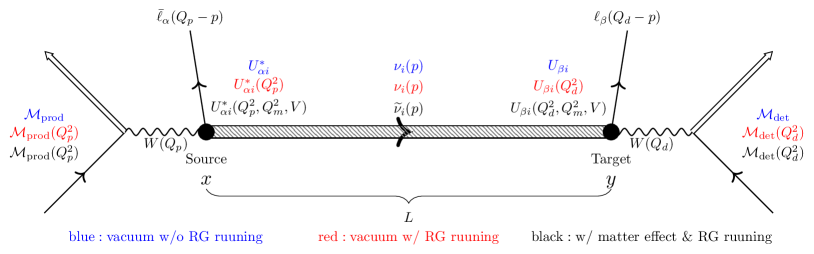
Fig. 1: The schematic plot for the QFT description of neutrino oscillation including three cases: 1) vacuum oscillation without considering RG running (blue); 2) vacuum oscillation with RG running (red); as well as 3) oscillation with both RG running and matter effect (black).

Note that the above QFT formalism for neutrino oscillation has two major differences with its quantum mechanics (QM) counterpart. In QM, the $\alpha$ flavor neutrino $\nu_{\alpha}$ is described by a quantum state $|\nu_{\alpha}\rangle\equiv a^{\dagger}_{\alpha}|0\rangle$ and similarly for the mass eigenstate $|\nu_{i}\rangle\equiv a_{i}^{\dagger}|0\rangle$. Since $\nu_{\alpha}\equiv\sum_{i}U_{\alpha i}\nu_{i}$, the neutrino operators $a_{\alpha}$ and $a_{i}$ (not $b_{\alpha}$ or $b_{i}$) have the same similarity transformation $a_{\alpha}=\sum_{i}U_{\alpha i}a_{i}$ according to $\nu\sim a+b^{\dagger}$. Then, the similarity transformation on the quantum states, $|\nu_{\alpha}\rangle=\sum_{i}U^{*}_{\alpha i}|\nu_{i}\rangle$, receives an extra complex conjugation. The second difference appears in the oscillation phase factor, $e^{-iE_{i}t}$, which has a minus sign according to the Schrodinger equation while its counterpart from the neutrino propagator in QFT is $e^{i|\mathbf{p}|L}$ without minus sign. With simultaneous presence of both differences, the oscillation probability derived in both QFT and QM formalism is the same.

3.2 Vacuum Oscillation with RG Running and Zero-Distance Effect

Note that physical variables such as the neutrino mixing parameters and masses depend on momentum transfer in the presence of RG running as mentioned in Sec. 2. Especially for a typical neutrino oscillation experiment, the momentum transfers in neutrino production, propagation, and detection processes are different from each other. However, since the neutrino mass receives negligible RG running effect [70, 71, 72, 73, 74, 75], the neutrino mass eigen-fields can be treated universally during the whole process. In this sense, the neutrino flavor eigen-fields become momentum transfer dependent via the mixing matrix $U(Q^{2})$, $\nu_{\alpha}(Q^{2})\equiv\sum_{i}U_{\alpha i}(Q^{2})\nu_{i}$. Besides the neutrino mixing matrices and neutrino flavor eigen-fields, quantum corrections can also generate a RG running effect on the gauge coupling $g$ of CC weak interactions, $g\rightarrow g(Q^{2})$ [75]. As shown in Fig. 1, the full transition matrix element for the vacuum oscillation with RG running effect can be obtained by replacing the relevant parameters in Eq. (3.6) with their $Q^{2}$-dependent counterparts,

$$\mathcal{T}=-\frac{i}{8\pi^{2}L}\int dp_{0}d^{4}xd^{4}y\mathcal{M}_{\rm det}(y,Q^{2}_{d})\left[\sum_{i}U_{\beta i}(Q^{2}_{d})e^{-i\frac{m_{i}^{2}}{2E_{\nu}}L}U^{*}_{\alpha i}(Q^{2}_{p})\right]\mathcal{M}_{\rm prod}(x,Q^{2}_{p}),$$ (3.8)

where the momentum transfers in the neutrino production and detection processes are defined as $Q^{2}_{p}$ and $Q^{2}_{d}$. Finally, the vacuum oscillation amplitude with the RG running effect receives a modification on the mixing matrix from Eq. (3.7),

$$\mathcal{A}^{\rm osc}_{\beta\alpha}=U_{\beta i}(Q^{2}_{d})e^{-iL\frac{m^{2}_{i}}{2E_{\nu}}}U^{\ast}_{\alpha i}(Q^{2}_{p}).$$ (3.9)

The oscillation amplitude and consequently the corresponding probability $P_{\alpha\beta}(E_{\nu},Q^{2}_{p},Q^{2}_{d})$ have dependence on the production and detection momentum transfers in addition to the neutrino energy.

The matrix elements $\mathcal{M}_{\rm prod}(x,Q^{2}_{p})$ and $\mathcal{M}_{\rm det}(y,Q^{2}_{d})$ absorb the $Q^{2}$-dependent gauge couplings $g(Q^{2}_{p})$ and $g(Q^{2}_{d})$, respectively. For simplicity, we focus on the running effect that enters the oscillation probability to emphasize its effect on the oscillation behaviors. However, the gauge coupling can also enter the oscillation probability through the matter effect as we elaborate later in Sec. 3.3.

From Eq. (3.9), an interesting effect emerges. The transition probability does not vanish in the zero-distance limit,

$$P_{\alpha\beta}=\left|\left[U(Q_{d}^{2})U^{\dagger}(Q_{p}^{2})\right]_{\beta\alpha}\right|^{2},$$ (3.10)

if the mixing matrices $U(Q^{2}_{p})$ and $U(Q^{2}_{d})$ in the production and detection processes mismatch with each other. On the other hand, the oscillation probability $P_{\alpha\beta}$ reduces to $\delta_{\alpha\beta}$ if $Q_{d}^{2}=Q^{2}_{p}$. The zero-distance transition probability can be explicitly calculated by using the standard PMNS parametrization [9],

$$U_{\rm PMNS}\equiv O_{23}P_{\delta_{D}}^{*}O_{13}P_{\delta_{D}}O_{12},$$ (3.11)

where $O_{ij}$ are the Euler rotation matrices and $P_{\delta_{D}}\equiv{\rm diag}\{1,1,e^{-i\delta_{D}}\}$. Since we mainly focus on the RG running of the Dirac CP phase $\delta_{D}$, we simply fix the other oscillation parameters except the CP phase and define the change of $\delta_{D}$ due to RG running as $\Delta\delta_{D}(Q^{2}_{d,p})\equiv\delta_{D}(Q^{2}_{d})-\delta_{D}(Q^{2}_{p})$, where $\delta_{p,d}\equiv\delta_{D}(Q^{2}_{p,d})$ represent the running CP phases in production and detection, respectively. Then the transition amplitude $U\left(Q_{d}^{2}\right)U^{\dagger}\left(Q_{p}^{2}\right)$ becomes,

$$\mathbb{1}+\frac{e^{-i\Delta\delta_{D}}-1}{2}\begin{pmatrix}2\sin^{2}{\theta_{r}}&e^{-i\delta_{p}}s_{a}\sin 2\theta_{r}&e^{-i\delta_{p}}c_{a}\sin 2\theta_{r}\\ e^{i\delta_{d}}s_{a}\sin 2\theta_{r}&-2e^{i\Delta\delta_{D}}s_{a}^{2}\sin^{2}\theta_{r}&-2e^{i\Delta\delta_{D}}s_{a}c_{a}\sin^{2}\theta_{r}\\ e^{i\delta_{d}}c_{a}\sin 2\theta_{r}&-2e^{i\Delta\delta_{D}}s_{a}c_{a}\sin^{2}\theta_{r}&-2e^{i\Delta\delta_{D}}c_{a}^{2}\sin^{2}\theta_{r}\end{pmatrix}.$$ (3.12)

It is interesting to see that it contains only the reactor ($\theta_{r}$) and atmospheric ($\theta_{a}$) mixing angles while the solar angle ($\theta_{s}$) does not appear at all. Then the explicit form of the zero-distance transition probability is obtained by putting the above expression into Eq. (3.10). For $\nu_{e}\rightarrow\nu_{e}$ and $\nu_{\mu}\rightarrow\nu_{e}$, the transition probabilities are,

$$P_{ee}(Q^{2}_{d,p})=1-\sin^{2}\left(\frac{\Delta\delta_{D}}{2}\right)\sin^{2}2\theta_{13},\quad P_{\mu e}(Q^{2}_{d,p})=\sin^{2}\left(\frac{\Delta\delta_{D}}{2}\right)s^{2}_{23}\sin^{2}2\theta_{13}\,.$$ (3.13)

Although these probabilities are independent of the Dirac CP phase itself, but are functions of the CP phase difference induced by the running effect. Most interestingly, the $P_{ee}$ oscillation probability that is typically independent of the Dirac CP phase has dependence on the CP phase difference induced by the RG running parameter $\Delta\delta_{D}$. The zero-distance effect is unique for identifying the running effect. On the experimental side, such an effect can be constrained using the data from the short-baseline (SBL) experiments as elaborated later in Sec. 5.

3.3 Neutrino Oscillation in Matter with RG Running

The neutrinos propagating in matter can experience that matter effect that arises from the forward scattering mediated by weak gauge bosons. It adds an additional matter potential matrix $V$ to the vacuum Hamiltonian $H_{0}$,

$$H\equiv H_{0}+V.$$ (3.14)

Note that the vacuum Hamiltonian $H_{0}\equiv M^{\dagger}M/2E_{\nu}$ is usually defined in the vacuum flavor basis $\nu_{\alpha}(Q^{2}_{\rm vac})$ where the momentum transfer is denoted as $Q^{2}_{\rm vac}$. Although there is no unique definition of $Q^{2}_{\rm vac}$ and its value is unknown, the introduction of this momentum transfer scale will not bring any problems since it will not appear in the final expression of oscillation probability as we show below. To ensure that the summation between $H_{0}$ and the matter potential matrix $V$ makes sense, the latter needs to be written in the same flavor basis as $H_{0}$.

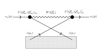
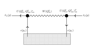
Fig. 2: The Feynman diagrams for the neutrino (left) and anti-neutrino (right) matter effects.

Recall that the neutrino flavor eigen-fields depend on the momentum transfer. Similarly the matter flavor basis is defined at the momentum transfer $Q^{2}_{m}$ of neutrino-matter interactions. As specifically shown in Fig. 2, the neutrino and anti-neutrino matter interactions are contributed by different Feynman diagrams. Although both arise from the $W$ boson mediation, their momentum transfers are different,

$$\nu:Q^{2}_{m}\equiv|(p_{\nu}-p_{e})^{2}|=|m^{2}_{e}-2m_{e}E_{\nu}|,\qquad\bar{\nu}:Q^{2}_{m}\equiv|(p_{\nu}+p_{e})^{2}|=|m^{2}_{e}+2m_{e}E_{\nu}|,$$ (3.15)

which should not be a vanishing value as adopted in [75]. Between the neutrino and anti-neutrino modes, the momentum transfer $Q^{2}_{m}=|m^{2}_{e}\mp 2m_{e}E_{\nu}|$ differs. Consequently, the matter flavor eigen-fields with $Q^{2}_{m}$ dependence are no longer the same as their vacuum counterparts and the usual definition of the matter potential without considering RG running no longer holds.

The matter potential matrix should be diagonal in the matter flavor basis $\nu_{\alpha}(Q^{2}_{m})$,

$$V\equiv\begin{pmatrix}\sqrt{2}G_{F}n_{e}&0&0\\ 0&0&0\\ 0&0&0\end{pmatrix}.$$ (3.16)

To match with the vacuum Hamiltonian $H_{0}$, the matter potential matrix needs to be rotated to the vacuum flavor basis $\nu_{\alpha}(Q^{2}_{\rm vac})$. The connection between the vacuum ($\nu_{\alpha}(Q^{2}_{\rm vac})$) and matter ($\nu_{\alpha}(Q^{2}_{m})$) flavor eigen-fields is established through the commonly shared mass eigen-fields $\nu_{i}$, $\nu_{\alpha}(Q^{2})=\sum_{i}U_{\alpha i}(Q^{2})\nu_{i}$,

$$\nu_{\alpha}(Q^{2}_{m})=\sum_{i}U_{\alpha i}(Q^{2}_{m})\nu_{i}=\sum_{i\beta}U_{\alpha i}(Q^{2}_{m})U_{\beta i}^{\ast}(Q^{2}_{\rm vac})\nu_{\beta}(Q^{2}_{\rm vac}).$$ (3.17)

For convenience, we define $U(Q^{2}_{m},Q^{2}_{\rm vac})\equiv U(Q^{2}_{m})U^{\dagger}(Q^{2}_{\rm vac})$. Although the production, detection, and even the matter interaction processes involve different momentum transfers and hence should have different flavor eigen-fields, the vacuum mass eigen-fields is always defined for on-shell neutrinos. This property is based on the observation that the neutrino mass receives a very tiny RG running effect [70, 71, 72, 73, 74, 75]. Now the total Hamiltonian can be written in the common vacuum flavor eigen-fields ($\nu_{\alpha}(Q^{2}_{\rm vac})$) using the transformation between vacuum and matter flavor eigen-fields in Eq. (3.17), $H=M^{\dagger}M/2E_{\nu}+U^{\dagger}(Q^{2}_{m},Q^{2}_{\rm vac})VU(Q^{2}_{m},Q^{2}_{\rm vac})$. After a similarity transformation $H\rightarrow U^{\dagger}(Q^{2}_{\rm vac})HU(Q^{2}_{\rm vac})$, the total Hamiltonian can be written in the vacuum mass eigen-fields,

$$H=\frac{M_{d}^{2}}{2E_{\nu}}+U^{\dagger}(Q^{2}_{m})VU(Q^{2}_{m}),$$ (3.18)

where $M_{d}^{2}\equiv U^{\dagger}(Q^{2}_{\rm vac})M^{\dagger}MU(Q^{2}_{\rm vac})\equiv{\rm diag}\{m^{2}_{1},m^{2}_{2},m^{2}_{3}\}$ is the diagonal mass matrix in vacuum. The undetermined $Q^{2}_{\rm vac}$ does not appear in this Hamiltonian anymore and will not affect the oscillation probability.

The diagonalization of the total Hamiltonian will give the effective mass eigen-fields $\tilde{\nu}_{i}$ with the effective masses $\widetilde{m}_{i}$ during the propagation by one unitary matrix $U(Q^{2}_{m},V)$,

$$H_{d}\equiv U^{\dagger}(Q^{2}_{m},V)HU(Q^{2}_{m},V)\equiv{\rm diag}\left\{\frac{\widetilde{m}_{1}^{2}}{2E_{\nu}},\frac{\widetilde{m}_{2}^{2}}{2E_{\nu}},\frac{\widetilde{m}_{3}^{2}}{2E_{\nu}}\right\}.$$ (3.19)

The vacuum mass eigen-fields $\nu_{i}$ and the effective mass eigen-fields $\tilde{\nu}_{i}$ in matter are connected via the same unitary matrix $U(Q^{2}_{m},V)$, $\nu_{i}=\sum_{j}U_{ij}(Q^{2}_{m},V)\tilde{\nu}_{j}(Q^{2}_{m},V)$. It can reduce to $\nu_{i}=\widetilde{\nu}_{i}$ in the absence of matter potential $V$ as expected. Note that the matrix $U(Q^{2}_{m},V)$ is only used to diagonalize the total Hamiltonian.

To connect propagation with the production and detection processes, the relation between the effective mass eigen-fields $\widetilde{\nu}_{i}$ in matter and the production as well as detection flavor eigen-fields $\nu_{\alpha}(Q^{2}_{p,d})$ is needed. Since the production and detection flavor eigen-fields connect with the vacuum mass eigen-fields $\nu_{j}$ via $\nu_{\alpha}(Q^{2}_{p,d})=\sum_{i}U_{\alpha i}(Q^{2}_{p,d})\nu_{i}$, the effective mass eigen-fields correlate with the production and detection flavor eigen-fields,

$$\nu_{\alpha}(Q^{2}_{p,d})=\sum_{ij}U_{\alpha i}(Q^{2}_{p,d})U_{ij}(Q^{2}_{m},V)\tilde{\nu}_{j}(Q^{2}_{m},V)\equiv\sum_{\alpha}U_{\alpha j}(Q^{2}_{p,d},Q^{2}_{m},V)\tilde{\nu}_{j}(Q^{2}_{m},V),$$ (3.20)

where we define a unitary matrix $U(Q^{2}_{p,d},Q^{2}_{m},V)\equiv U(Q^{2}_{p,d})U(Q^{2}_{m},V)$ for convenience.

Now the oscillation formula for the vacuum case in Sec. 3.2 can easily extend to the matter case. Reviewing the whole oscillation process shown in Fig. 1, the neutrino is first produced with flavor $\alpha$, which decomposes into effective neutrino mass eigen-fields with an associated matrix $U^{\ast}_{\alpha i}(Q^{2}_{p},Q^{2}_{m},V)$. After propagating a macroscopic spatial distance $L$, each effective mass eigen-field with the effective mass $\widetilde{m}_{i}$ receives a phase factor, $e^{-iL\frac{\widetilde{m}^{2}_{i}}{2E_{\nu}}}$. Finally, the effective mass eigen-fields combine linearly with coefficients $U_{\beta i}(Q^{2}_{d},Q^{2}_{m},V)$ to flavor eigen-fields $\nu_{\beta}(Q^{2}_{d})$ to be detected. Then the net effect gives the oscillation amplitude,

$$\mathcal{A}_{\beta\alpha}^{\rm osc}\equiv\sum_{i}U_{\beta i}(Q^{2}_{d},Q^{2}_{m},V)e^{-iL\frac{\widetilde{m}^{2}_{i}}{2E_{\nu}}}U_{i\alpha}^{\dagger}(Q^{2}_{p},Q^{2}_{m},V)\,.$$ (3.21)

The above amplitude reduces to the vacuum one when the matter potential is vanishing with $U(Q^{2}_{p,d},Q^{2}_{m},V)\rightarrow U(Q^{2}_{p,d})$ and $\tilde{m}_{i}\rightarrow m_{i}$ as expected. Different from the vacuum case, the oscillation amplitude with matter effect involves one more momentum transfer $Q^{2}_{m}$ which is not negligible when considering the RG running effect. Besides, the gauge coupling enters the oscillation amplitude/probability through the matter potential term of the total Hamiltonian as shown in Eq. (3.18). For simplicity, we do not consider the RG running effect on the coupling constant but only the mixing parameters in this paper.

3.4 Numerical Illustration of the RG Running Effect

To illustrate the RG running effect on the neutrino oscillation probabilities (dashed, dotted, and dash-dotted curves),

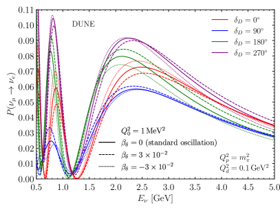
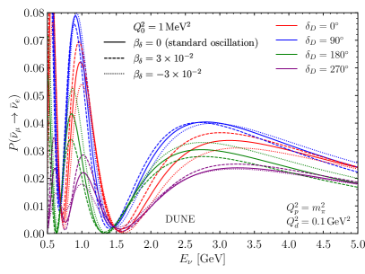
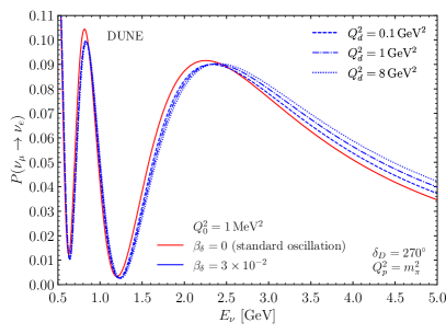
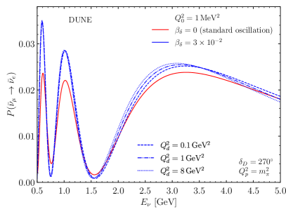
Fig. 3: The oscillation probabilities as a function of the neutrino energy $E_{\nu}$ for the DUNE configuration with $L=1284.9\,$km and $\rho=2.848\,$g/cm³. Upper left: The $\nu_{\mu}\rightarrow\nu_{e}$ oscillation probabilities for the neutrino mode with $\beta_{\delta}=0$ (solid), $3\times 10^{-2}$ (dashed), and $-3\times 10^{-2}$ (dotted). Note that $\beta_{\delta}=0$ corresponds to the standard oscillation probabilities without RG running effect. Four different CP values $\delta_{D}=0^{\circ}$ (red), $90^{\circ}$ (blue), $180^{\circ}$ (green), and $270^{\circ}$ (purple) are chosen for illustration. Upper right: Same as the left but for the anti-neutrino mode $\bar{\nu}_{\mu}\rightarrow\bar{\nu}_{e}$. Lower left: The $\nu_{\mu}\rightarrow\nu_{e}$ oscillation probabilities with fixed CP value $\delta_{D}=270^{\circ}$ for $Q^{2}_{d}=0.1\,$GeV² (dashed blue), $1\,$GeV² (dot-dashed blue), and 8 GeV² (blue dotted). Lower right: Same as the left but for the anti-neutrino mode $\bar{\nu}_{\mu}\rightarrow\bar{\nu}_{e}$.

we compare with the standard result (solid curves) in Fig. 3. For all panels, we take the DUNE configuration with $L=1284.9\,$km, $E_{\nu}\in[0.5\,\rm{GeV},5\,\rm{GeV}]$, and production momentum transfer $Q^{2}_{p}=(p_{\nu_{\mu}}+p_{\mu})^{2}=m^{2}_{\pi}$ for neutrinos produced from pion decay. However, the detection momentum transfer $Q^{2}_{d}$ depends on the interaction with the target and its value can vary a lot as we show below in Sec. 4.1. The upper left/right panel shows the RG running effect on the $\nu_{\mu}\rightarrow\nu_{e}/\bar{\nu}_{\mu}\rightarrow\bar{\nu}_{e}$ oscillation probabilities with three $\beta_{\delta}$ (defined in Eq. (2.2)) values: $\beta_{\delta}=0$ (without RG running), $-3\times 10^{-2}$, and $3\times 10^{-2}$. For both panels, there are three oscillation peaks which locate at $E_{\nu}\sim 0.5$, $0.8$, $2.5\,$GeV, respectively. Among these three oscillation peaks, the 2.5 GeV one contributes most to the event rate at DUNE since the DUNE neutrino spectrum peaks in this region. For neutrino energies within $[2\,\rm{GeV},3\,\rm{GeV}]$, the relative oscillation probability difference ($\equiv|P(\beta_{\delta}\neq 0)-P(\beta_{\delta}=0)|/P(\beta_{\delta}=0)$) can reach percentage level and has a similar size as the CP effect. Hence the RG running effect on neutrino oscillation probabilities is not negligible.

In the lower panels of Fig. 3, we study the impact on oscillation probabilities with three different $Q^{2}_{d}$ values: $Q^{2}_{d}=0.1\,$GeV², 1 GeV², and 8 GeV². For the neutrino mode, the numerical result shows that the three blue curves with different $Q^{2}_{d}$ values are close to each other for $E_{\nu}$ below $2.5\,$GeV and can be distinguished for $E_{\nu}$ above $2.5\,$GeV. However, for the anti-neutrino mode, these curves are distinguishable for $E_{\nu}$ from 2 GeV up to 5 GeV. Hence for a real neutrino experiment like DUNE, the momentum transfer should be carefully reconstructed in order to study the RG running effect as we elaborate below.

4 CP Phase Sensitivity Reduction at DUNE

A major concern is that the neutrino CP measurement will suffer from the RG running effect. As mentioned above, the oscillation probability with RG running can vary a lot with the neutrino energy $E_{\nu}$ and the detection momentum transfer $Q^{2}_{d}$. Such effect appears when the two momentum transfers in neutrino production ($Q^{2}_{p}$) and detection ($Q^{2}_{d}$) mismatch. The larger mismatch the larger RG running effect. With large neutrino energy, DUNE can provide a large detection momentum transfer and hence a large RG running effect. So we take DUNE as an example to quantitatively study the impact.

4.1 Neutrino Energy and Momentum Transfer Reconstructions

The production momentum transfer has a fixed value as the pion mass $Q^{2}_{p}=m_{\pi}^{2}$ since most DUNE neutrinos are generated through pion decay [82]. To evaluate the oscillation probability $P_{\alpha\beta}(E_{\nu},Q^{2}_{p},Q^{2}_{d})$ with the RG running effect, one still needs to reconstruct the neutrino energy $E_{\nu}$ and the detection momentum transfer $Q^{2}_{d}$. The neutrino energy, $E^{\rm rec}_{\nu}\equiv E^{\rm rec}_{\ell}+E^{\rm rec}_{\rm had}$, is reconstructed from the deposited lepton ($E^{\rm rec}_{\ell}$) and hadronic ($E^{\rm rec}_{\rm had}$) energies [23]. On the other hand, the reconstructed detection momentum transfer $Q^{2}_{\rm rec}$ correlates to not just the reconstructed neutrino energy $E^{\rm rec}_{\nu}$, but also the measured charged lepton energy $E^{\rm rec}_{\ell}$ and the measured lepton scattering angle $\theta^{\rm rec}_{\ell}$,

$$Q^{2}_{\rm rec}\equiv|(p^{\rm rec}_{\nu}-p^{\rm rec}_{\ell})^{2}|=2E^{\rm rec}_{\nu}(E^{\rm rec}_{\ell}-|{\boldsymbol{p}}^{\rm rec}_{\ell}|\cos\theta^{\rm rec}_{\ell})-m^{2}_{\ell},$$ (4.1)

where $m_{\ell}$ is the lepton mass. Note that the lepton momentum cannot be directly reconstructed but needs to be obtained from the reconstructed lepton energy, $|{\boldsymbol{p}}_{\ell}|^{\rm rec}\equiv\sqrt{(E^{\rm rec}_{\ell})^{2}-m^{2}_{\ell}}$. In total, three observables (the reconstructed lepton energy $E^{\rm rec}_{\ell}$, the hadronic energy $E^{\rm rec}_{\rm had}$, and the measured lepton scattering angle $\theta^{\rm rec}_{\ell}$) are needed.

4.1.1 Energy Reconstruction

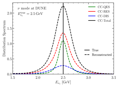
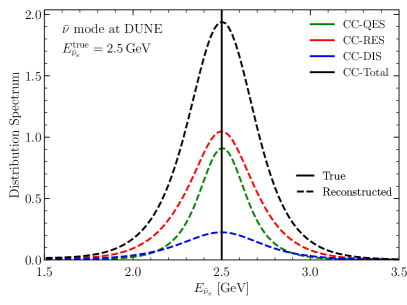
Fig. 4: Left: The reconstructed energy ($E^{\rm rec}_{\nu}=E^{\rm rec}_{\ell}+E^{\rm rec}_{\rm had}$) distribution of a 2.5 GeV $\nu_{e}$ neutrino at the DUNE detector for different CC scattering processes: QES (green), RES (red), and DIS (blue). The combined total spectrum is plotted in black color. Note that the total spectrum is normalized and the others are weighted by their corresponding cross sections. Right: Same as the left panel but for the anti-neutrino mode.

We use GENIE [83, 84] to generate the neutrino-Argon scattering events and simulate the neutrino energy reconstruction at DUNE. Note that the neutrino energy does not fully deposit as visible energy and some is missing. In a liquid Argon Time Projection Chamber (TPC) such as the DUNE far detectors, the energy is reconstructed via the tracks left by the final-state particles. Those tracks with deposited energy below the detector threshold cannot be measured. Moreover, some final-state particles such as neutrino cannot leave a track and hence is not measurable either. These contribute as missing energy [85]. To precisely reconstruct the neutrino energy, we add a constant value, $\langle E_{\rm mis}\rangle$, as correction to calibrate the energy reconstruction by taking into account the average missing energy, $\langle E_{\rm mis}\rangle=30$ MeV, $20$ MeV, and $20$ MeV for the QES, RES, and DIS scattering processes, respectively.

In addition, the charged lepton ($E_{\ell}^{\rm rec}$) and hadronic ($E_{\rm had}^{\rm rec}$) energies are smeared around their respective true values. The Gaussain smearing resolution of each detectable particle is determined by the best reconstruction case in [85] as summarized in Table 1.

Particle	Energy Resolution ($\sigma/E$) at DUNE
$\pi^{\pm}$	15%
$\mathrm{e}^{\pm}/\gamma$	1.5%
$p$	$\mathrm{p}<400\,\mathrm{MeV}/\mathrm{c}:4\%$ $\mathrm{p}>400\,\mathrm{MeV}/\mathrm{c}:10\%\oplus 3.1\%/\sqrt{E}\,[\mathrm{GeV}]$
$n$	$40\%/\sqrt{E}\,[\mathrm{GeV}]$
other	$5\%\oplus 30\%/\sqrt{E}\,[\mathrm{GeV}]$

Table 1: The energy resolutions for detectable particles obtained by fitting to the best reconstruction case in [85].

Fig. 4 shows the reconstructed spectrum of CC events for 2.5 GeV $\nu_{e}$ and $\bar{\nu}_{e}$, respectively. Note that the energy reconstruction for the CC-QES process has a better performance than the other two CC-RES and CC-DIS processes, since the deposited energy for CC-QES mostly comes from the charged leptons which have a better resolution than the other particles produced in the RES and DIS processes.

4.1.2 Momentum Transfer Reconstruction in Terms of Scattering Angle

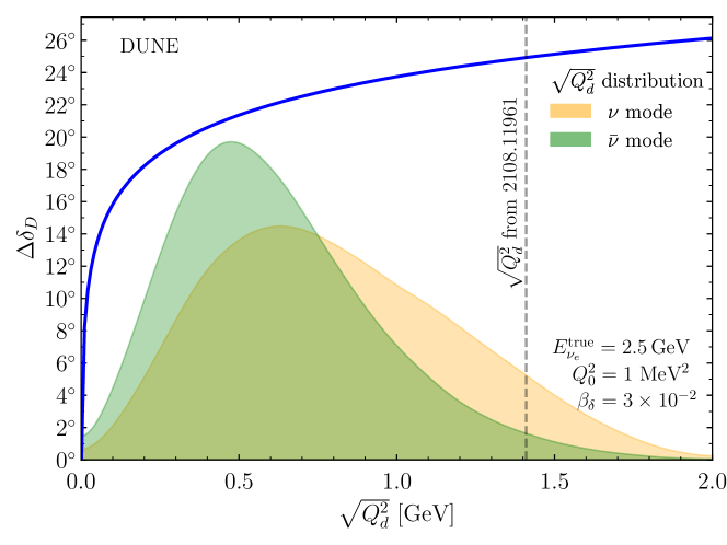
Fig. 5: The CP phase change $\Delta\delta_{D}\equiv\beta_{\delta}\ln\left(\left|Q^{2}/Q^{2}_{0}\right|\right)$ induced by the RG running effect with $Q^{2}_{0}=1$ MeV² and $\beta_{\delta}=3\times 10^{-2}$ as function of the detection momentum transfer $\sqrt{Q^{2}_{d}}$. The $\sqrt{Q^{2}_{d}}$ distributions for $\nu_{e}-$Argon scattering events are shown with the orange and green shaded regions for the neutrino and anti-neutrino modes, respectively. For comparison, the fixed $\sqrt{Q^{2}_{d}}\approx 1.4\,$GeV from $Q^{2}_{d}=2m_{N}E_{\nu}^{2}/(2E_{\nu}+m_{N})$ is presented by the vertical gray dashed line.

As mentioned above, the production momentum transfer $Q^{2}_{p}$ has fixed value as the pion mass, $Q^{2}_{p}=m_{\pi}^{2}$. For the detection momentum transfer $Q^{2}_{d}$, the previous work [75] also uses a fixed value, $Q^{2}_{d}=2m_{N}E_{\nu}^{2}/(2E_{\nu}+m_{N})$, where $m_{N}$ is the target nucleon mass. Then a 2.5 GeV neutrino corresponds to $\sqrt{Q^{2}_{d}}\approx 1.4$ GeV. However, the momentum transfer of CC events is not fixed but follows a distribution shown as the shaded regions in Fig. 5. The estimated momentum transfer value actually locates at the tail of the distribution and is at least two times of the mean momentum transfer that is around $0.5\sim 0.7$ GeV. To see the running effect on the Dirac CP phase, we show the CP phase change $\Delta\delta_{D}$ $(\equiv\beta_{\delta}\ln\left(\left|Q^{2}/Q^{2}_{0}\right|\right)$ induced by RG running with the blue curve in Fig. 5. The value of $\Delta\delta_{D}$ varies a lot throughout the $\sqrt{Q^{2}_{d}}$ distribution region. Especially for $\sqrt{Q^{2}_{d}}<0.5\,$GeV, the corresponding $\Delta\delta_{D}$ has a large variation and is quite different from its counterpart adopted in the previous work. Therefore, an event-by-event reconstruction of the detection momentum transfer according to Eq. (4.1) is necessary at DUNE.

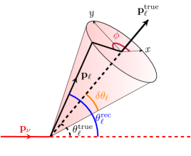
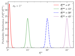
Fig. 6: Left: The schematic plot for the charged lepton scattering angle $\theta^{\rm rec}_{\ell}$ reconstruction. With $\theta_{\ell}^{\rm true}$ being the true scattering angle between the final-state lepton ${\bf p}_{\ell}^{\rm true}$ and incoming neutrino ${\bf p}_{\nu}$ momenta, $\delta\theta_{\ell}$ is the opening angle between the measured lepton $\bf{p}_{\ell}$ and the true one ${\bf p}_{\ell}^{\rm true}$. Moreover, the azimuthal angle $\phi$ for the measured lepton momentum surrounding the true lepton momentum is randomly distributed in the range of [0, 2$\pi$). Right: The probability distribution of the lepton scattering angle $\theta^{\rm rec}_{\ell}$ with four true scattering angles: $\theta^{\rm true}_{\ell}=0^{\circ}$ (solid red), $15^{\circ}$ (dashed green), $30^{\circ}$ (dot-dashed blue), and $45^{\circ}$ (dotted purple). We use the angular resolution $\sigma_{\theta}=1^{\circ}$ from the DUNE CDR result.

In order to reconstruct the detection momentum transfer $Q^{2}_{d}$, the scattering angle reconstruction plays an important role. Note that the Gaussian smearing of the true scattering angle cannot be directly used to simulate the measured angle due to the geometry effect that is illustrated in the left panel of Fig. 6. The incoming neutrino with momentum ${\bf p}_{\nu}$ interacts with the detector target which is marked as the black dot and a final-state charged lepton with true momentum ${\bf p}_{\ell}^{\rm true}$ is produced. Since the detector has a limited angular resolution, it measures the lepton momentum ${\bf p}_{\ell}$ with an opening angle $\delta\theta_{\ell}$ from the true one. The value of $\delta\theta_{\ell}$ follows a Gaussian distribution that depends on the detector angular resolution $\sigma_{\theta}$. In addition, the azimuthal angle $\phi$ for the measured lepton momentum surrounding the true lepton momentum distributes randomly in [0, $2\pi$) and affects the measured lepton scattering angle $\theta^{\rm rec}_{\ell}$. We follow the analytical method in [86] where the probability density $P(\theta^{\rm rec}_{\ell}|\theta_{\ell}^{\rm true})$ for obtaining the measured scattering angle $\theta^{\rm rec}_{\ell}$ from the given true one $\theta_{\ell}^{\rm true}$ is,

$$P(\theta^{\rm rec}_{\ell}|\theta_{\ell}^{\rm true})=\frac{1}{2\pi}\int^{\pi}_{0}\frac{P(\delta\theta_{\ell})\sin\theta^{\rm rec}_{\ell}}{\sqrt{\sin^{2}\theta^{\rm true}_{\ell}\sin^{2}\delta\theta_{\ell}-(\cos\theta^{\rm true}_{\ell}\cos\delta\theta_{\ell}-\cos\theta^{\rm rec}_{\ell})^{2}}}d\delta\theta_{\ell}\,.$$ (4.2)

In the above expression, $P(\delta\theta_{\ell})\equiv\sin\delta\theta_{\ell}/N(\sigma_{\theta})\exp\left[-1/2\left(\delta\theta_{\ell}/\sigma_{\theta}\right)^{2}\right]$ is the distribution function of the opening angle $\delta\theta_{\ell}$ with $\sigma_{\theta}$ being the detector angular resolution and $N(\sigma_{\theta})$ the normalization factor. In our analysis, we take $\sigma_{\theta}=1^{\circ}$ from the DUNE Conceptual Design Report (CDR) result [23]. In the right panel of Fig. 6, we show the probability density for the measured scattering angle $\theta^{\rm rec}_{\ell}$ with four true scattering angle values $\theta^{\rm true}_{\ell}=0^{\circ}$, $15^{\circ}$, $30^{\circ}$, and $45^{\circ}$ for illustration. For $\theta^{\rm true}_{\ell}\gg\sigma_{\theta}$, the smeared scattering angle closely follows a Gaussian distribution while the shape is significantly distorted when the $\theta^{\rm true}_{\ell}$ value is comparable with its angular resolution $\sigma_{\theta}$.

Finally, the combination of $E^{\rm rec}_{\nu},E^{\rm rec}_{\ell}$, and $\theta^{\rm rec}_{\ell}$ through Eq. (4.1) reconstructs the detection momentum transfer $Q^{2}_{d}$. Fig. 7 shows the $\sqrt{Q^{2}_{d}}$ distribution of a 2.5 GeV neutrino scattering with Argon target for different CC scattering processes. The reconstructed momentum transfer distributions (dashed) are in good agreement with the true ones (solid), although the neutrino energy reconstruction is far from being perfect as shown in Fig. 4.

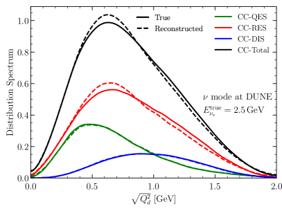
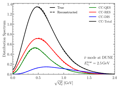
Fig. 7: Left: The reconstructed momentum transfer $\sqrt{Q^{2}_{d}}$ distribution of a 2.5 GeV $\nu_{e}$ neutrino at the DUNE detector for different CC scattering processes: QES (green), RES (red), and DIS (blue). The total spectrum (black) is normalized to 1 while the others are weighted by their corresponding cross sections. Right: Same as the left panel but for the anti-neutrino mode.

4.1.3 4-D Transfer Table for Energy and Momentum Transfer

As mentioned above, the detector energy and angular resolutions will smear the true values $(E^{{\rm true},i}_{\nu},Q^{2}_{{\rm true},j})$ into their reconstructed counterparts $(E_{\nu}^{{\rm rec},i^{\prime}},Q^{2}_{{\rm rec},j^{\prime}})$ with $i$, $j$, $i^{\prime}$, and $j^{\prime}$ being the indices of their respective bins. Given a true neutrino energy and a true momentum transfer, the transfer between the true and reconstructed values is summarized in a 4-D transfer table $T^{\prime}_{iji^{\prime}j^{\prime}}$,

$$T^{\prime}_{iji^{\prime}j^{\prime}}\equiv\frac{\Delta N(E^{{\rm true},i}_{\nu},Q^{2}_{{\rm true},j};E_{\nu}^{{\rm rec},i^{\prime}},Q^{2}_{{\rm rec},j^{\prime}})}{N_{\rm total}(E^{{\rm true},i}_{\nu},Q^{2}_{{\rm true},j})}.$$ (4.3)

Here $\Delta N(E^{{\rm true},i}_{\nu},Q^{2}_{{\rm true},j};E_{\nu}^{{\rm rec},i^{\prime}},Q^{2}_{{\rm rec},j^{\prime}})$ is the simulated event number within the $i^{\prime}$-th reconstructed energy bin and the $j^{\prime}$-th reconstructed momentum transfer bin for the given $i$-th true neutrino energy bin and the $j$-th true momentum transfer bin, while $N_{\rm total}(E^{{\rm true},i}_{\nu},Q^{2}_{{\rm true},j})$ is the total simulated event number of the given $i$-th true neutrino energy bin and $j$-th true momentum transfer bin. The transfer table element is the probability for finding the reconstructed values ($E_{\nu}^{{\rm rec},i^{\prime}},Q^{2}_{{\rm rec},j^{\prime}}$) after smearing their respective true values ($E^{{\rm true},i}_{\nu},Q^{2}_{{\rm true},j}$). Such effective transfer table satisfies the probability conservation condition, $\sum_{i^{\prime}j^{\prime}}T^{\prime}_{iji^{\prime}j^{\prime}}=1$, as expected. Moreover, the transfer table enters the reconstructed event rates calculation as elaborated below.

4.2 Extended GLoBES Simulation with both Energy and Momentum Transfer

As pointed out around Eq. (3.9), the oscillation probability has momentum transfer dependence. In the presence of the RG running effect, the neutrino oscillation event rate is a function of not just the neutrino energy ($E_{\nu}$) but also the momentum transfers ($Q^{2}_{p}$ and $Q^{2}_{d}$). With the production momentum transfer ($Q^{2}_{p}$) typically fixed by the parent meson masses, the event rate is still a two-dimensional distribution of the neutrino energy ($E_{\nu}$) and the detection momentum transfer ($Q^{2}_{d}$).

The GLoBES [87, 88] simulation for fixed baseline experiments with one-dimensional event rate needs to be extended in order to incorporate the RG running effect. The two-dimensional binning approach with neutrino energy and zenith angle (baseline length) dependence has been used in the atmospheric neutrino oscillation analysis [89, 90]. We adopt similar approach by breaking the 2-D event rate $d^{2}N/dE_{\nu}dQ^{2}_{d}$ into multiple glb experimental profiles each with a fixed $Q^{2}_{d}$ and merging them in the end.

• GLoBES simulation: With a fixed $Q^{2}_{d}$ for each glb profile, the oscillation probability $P_{\alpha\beta}(E_{\nu}^{{\rm true},i},Q^{2}_{{\rm true},j})$ with the RG running effect in Sec. 3.3 taken into account and the corresponding event spectrum can be calculated in the usual way by GLoBES,

  $$\frac{dN^{\rm true}}{dE_{\nu}^{{\rm true},i}}\Bigg{|}_{Q^{2}_{{\rm true},j}}\equiv N^{\rm target}\phi_{\alpha}(E_{\nu}^{{\rm true},i})P_{\alpha\beta}(E_{\nu}^{{\rm true},i},Q^{2}_{{\rm true},j})\sigma_{\beta}(E_{\nu}^{{\rm true},i}),$$ (4.4)

  where $N^{\rm target}$ is the normalization factor including the information of running time, detector size, and the baseline length. Both the $\alpha$-flavor neutrino flux $\phi_{\alpha}(E_{\nu}^{{\rm true},i})$ and $\beta$-flavor detection cross section $\sigma_{\beta}(E_{\nu}^{{\rm true},i})$ are functions of the true neutrino energy $E_{\nu}^{{\rm true},i}$ for the $i$-th bin.

  Since the neutrino energy $E_{\nu}$ and detection momentum transfer $Q^{2}_{d}$ are reconstructed altogether, their smearing interleaves with each other and cannot be separated. So we first extract from GLoBES the event numbers at the true neutrino energy level,

  $${\rm GLB}_{j}:\quad N^{{\rm GLB}_{j}}_{i}=\frac{dN^{\rm true}}{dE_{\nu}^{{\rm true},i}}\Bigg{|}_{Q^{2}_{{\rm true},j}}\Delta E_{i}^{{\rm true},i},$$ (4.5)

  for the $j$-th glb experimental profile without smearing.

• Implementing the momentum transfer distribution by hand: Although GLoBES automatically incorporates the total cross section $\sigma(E_{\nu}^{{\rm true},i})$ in the event rate calculation according to Eq. (4.4), the differential spectrum with respect to the momentum transfer $Q^{2}_{d}$ is still missing. One needs to multiply the extracted event rate $N^{{\rm GLB}_{j}}_{i}$ with a normalized differential cross section $d\sigma_{\beta}/(\sigma_{\beta}dQ^{2}_{{\rm true},j})$ by hand. The event numbers among different glb profiles are then reshuffled into,

  $$N_{ij}\equiv N^{{\rm GLB}_{j}}_{i}\times\left(\frac{d\sigma_{\beta}}{\sigma_{\beta}dQ^{2}_{{\rm true},j}}\right)\Bigg{|}_{E^{{\rm true},i}_{\nu}}\Delta Q^{2}_{{\rm true},j},$$ (4.6)

  weighted by the momentum transfer bin size $\Delta Q^{2}_{{\rm true},j}$. The product of the normalized differential cross section and the true momentum transfer bin size can be simulated by GENIE as, $d\sigma_{\beta}/(\sigma_{\beta}dQ^{2}_{{\rm true},j})|_{E^{{\rm true},i}_{\nu}}\Delta Q^{2}_{{\rm true},j}=\Delta N(E^{{\rm true},i}_{\nu},Q^{2}_{{\rm true},j})/N(E^{{\rm true},i}_{\nu})$, as a ratio between the event number within the $j$-th true momentum transfer bin and the total one for a given true energy.

  Note that the two variables $N^{{\rm GLB}_{j}}_{i}$ and $N_{ij}$ have different physical meanings. While $N^{{\rm GLB}_{j}}_{i}$ is the event number within the $i$-th energy bin for the $j$-th glb profile that carries the momentum transfer dependence in the oscillation probability but no information about the momentum transfer distribution, the event number $N_{ij}$ within the $i$-th energy and $j$-th momentum transfer bin also includes the differential momentum transfer distribution. The essential difference between these two variables is having the momentum transfer distribution or not. Nevertheless, the $j$ index of $N^{{\rm GLB}_{j}}_{i}$ cannot be simply omitted since the oscillation probability has momentum transfer dependence. To make this tricky point explicit, we add $j$ as an upper index for $N^{{\rm GLB}_{j}}_{i}$ and a lower one for $N_{ij}$.

• Detector resolution and smearing: The normalized differential cross section in the 2-D true event rate calculation Eq. (4.6) cannot be automatically carried out in GLoBES and needs to be implemented by hand. In addition, the 4-D transfer table $T^{\prime}_{iji^{\prime}j^{\prime}}$ defined in Eq. (4.3) also needs to be implemented by hand with multiple glb profiles. For convenience, we combine these two terms into a single effective 4-D transfer table,

  $$N_{i^{\prime}j^{\prime}}\equiv\sum_{ij}N_{ij}\times T^{\prime}_{iji^{\prime}j^{\prime}}\equiv\sum_{ij}N^{{\rm GLB}_{j}}_{i}\times T_{iji^{\prime}j^{\prime}},$$ (4.7)

  where $N_{i^{\prime}j^{\prime}}$ is the event number in the $i^{\prime}$-th reconstructed energy and $j^{\prime}$-th reconstructed momentum transfer bin. Instead of using the $T^{\prime}_{iji^{\prime}j^{\prime}}$ Eq. (4.3), the event rate $N^{{\rm GLB}_{j}}_{i}$ extracted from GLoBES is directly related to the reconstructed event rate $N_{i^{\prime}j^{\prime}}$ with,

  $$T_{iji^{\prime}j^{\prime}}\equiv\left(\frac{d\sigma_{\beta}}{\sigma_{\beta}dQ^{2}_{{\rm true},j}}\right)\Bigg{|}_{E^{{\rm true},i}_{\nu}}\times\Delta Q^{2}_{{\rm true},j}\times T^{\prime}_{iji^{\prime}j^{\prime}}=\frac{\Delta N(E^{{\rm true},i}_{\nu},Q^{2}_{{\rm true},j};E_{\nu}^{{\rm rec},i^{\prime}},Q^{2}_{{\rm rec},j^{\prime}})}{N_{\rm total}(E^{{\rm true},i}_{\nu})},$$ (4.8)

  where $N_{\rm total}(E^{{\rm true},i}_{\nu})$ is the total event number for the given $i$-th true neutrino energy bin. The effective transfer table includes three terms: the normalized differential cross section $d\sigma_{\beta}/(\sigma_{\beta}dQ^{2}_{{\rm true},j})|_{E^{{\rm true},i}_{\nu}}$, the bin size $\Delta Q^{2}_{{\rm true},j}$, and the smearing transfer table $T^{\prime}_{iji^{\prime}j^{\prime}}$, which can be combined into a single simulation.

  In our simulation, we first use GENIE to generate $10^{6}$ neutrino-Ar scattering events for the true energy $E^{{\rm true},i}_{\nu}$ at the center of each bin. We then reconstruct event by event the neutrino energy and momentum transfer after smearing according to the detector energy and angular resolutions as discussed in Sec. 4.1. For the true/reconstructed energy, we take a 0.25 GeV bin size from 0.5 to 5 GeV. On the other hand, the true/reconstructed momentum transfer uses $\sqrt{Q^{2}_{d}}$ instead of $Q^{2}_{d}$ with 25 bins from 0 to $2\sqrt{2}\,$GeV since $Q^{2}_{d}$ distributes mainly at small values as shown in Fig. 7. Finally, we bin the events into a histogram with variables $(E_{\nu}^{\rm true},Q^{2}_{\rm true};E_{\nu}^{\rm rec},Q^{2}_{\rm rec})$ and divide the event number in each bin by the total event number to obtain the $T_{iji^{\prime}j^{\prime}}$ defined in Eq. (4.8). After these, we calculate the 2-D event rates according to Eq. (4.7) and feed them back into GLoBES for $\chi^{2}$ analysis to take full advantage.

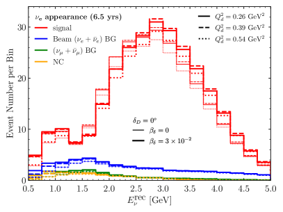
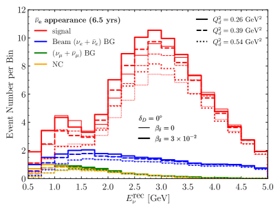
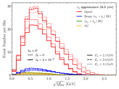
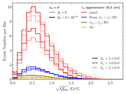
Fig. 8: Upper Panels: The reconstructed appearance event rates as a function of the reconstructed neutrino energy $E_{\nu}^{\rm rec}$ with detection momentum transfer $Q^{2}_{d}=0.26\,$GeV² (solid), $0.39\,$GeV² (dashed), and $0.54\,$GeV² (dotted) for the neutrino $\nu_{e}$ (upper left) and anti-neutrino $\bar{\nu}_{e}$ (upper right) modes. Lower Panels: The reconstructed appearance event rates as a function of $\sqrt{Q^{2}_{\rm rec}}$ with $E_{\nu}=2.125\,$GeV (solid), $2.625\,$GeV (dashed), and $3.125\,$GeV (dotted) for the neutrino $\nu_{e}$ (lower left) and anti-neutrino $\bar{\nu}_{e}$ (lower right) modes. For all panels, the event rates are divided into four components: the signal (red), the intrinsic $\nu_{e}+\bar{\nu}_{e}$ beam background (blue), the $\nu_{\mu}+\bar{\nu}_{\mu}$ beam background (green), and the neutral current background (orange). We take $\delta_{D}=0^{\circ}$ and a 6.5 years of running time for each neutrino and anti-neutrino mode to make illustration.

4.3 Event Rate and CP Phase Sensitivity at DUNE

Fig. 8 shows the event rates at DUNE as function of the reconstructed neutrino energy $E_{\nu}^{\rm rec}$ (upper panels) or momentum transfer $\sqrt{Q^{2}_{\rm rec}}$ (lower panels) for both neutrino (left panels) and anti-neutrino (right panels) modes. The event rate difference between the thin and thick lines induced by the RG running effect can reach percentage level. This happens for not just the signal (red lines) but the various background event rates since all channels are subject to the oscillation probabilities. The most prominent channel is the beam $\nu_{e}+\bar{\nu}_{e}$ background that is modulated by $P_{ee}$. As pointed out earlier at the end of Sec. 3.2, $P_{ee}$ is no longer independent of the Dirac CP phase $\delta_{D}$ as usually expected but becomes a function of the CP phase difference $\Delta\delta_{D}$ induced by the RG running effect. The largest variation occurs in the ranges $[1.5,4.5]$/$[1.25,3.5]\,\rm{GeV}$ of $E_{\nu}^{\rm rec}$ and $[0.2,1.5]$/$[0.2,1.2]\,\rm{GeV}$ of $\sqrt{Q^{2}_{\rm rec}}$ for the neutrino/anti-neutrino mode, respectively, around the peaks.

To further explore the features induced by the RG running effect, we show the relative difference of the two-dimensional signal event rate, $\Delta N/N\equiv\left(N_{\rm sig}\left(\beta_{\delta}=3\times 10^{-2}\right)-N_{\rm sig}(\beta_{\delta}=0)\right)/$ $N_{\rm sig}(\beta_{\delta}=0)$, on the $(E_{\nu}^{\rm rec},\sqrt{Q^{2}_{\rm rec}})$ plane in Fig. 9. Note that the distribution of $\Delta N/N$ is quite different between the neutrino (left) and anti-neutrino (right) modes. For the neutrino mode, the positive $\Delta N/N$ values distribute at $E_{\nu}^{\rm rec}\in[3.5,5]\,$GeV while the negative one within $E\in[1.5,2.5]\,$GeV. As for the anti-neutrino mode, the negative $\Delta N/N$ values mainly distribute at $E_{\nu}^{\rm rec}\in[1,1.75]\,$GeV for most $\sqrt{Q^{2}_{\rm rec}}$ and $E_{\nu}^{\rm rec}\in[3.5,4.75]\,$GeV for $\sqrt{Q^{2}_{\rm rec}}\in[0,1.2]\,$GeV, with the positive values in the remaining part. The RG running effect can be tested at the future LBL experiments such as DUNE. Unfortunately, since the genuine CP phase is undetermined, a degeneracy between the genuine CP phase $\delta_{D}$ and the RG running parameter $\beta_{\delta}$ arises which reduces the CP phase sensitivity. The structure in the two-dimensional $(E_{\nu}^{\rm rec},\sqrt{Q^{2}_{\rm rec}})$ distributions may help to disentangle the degeneracy.

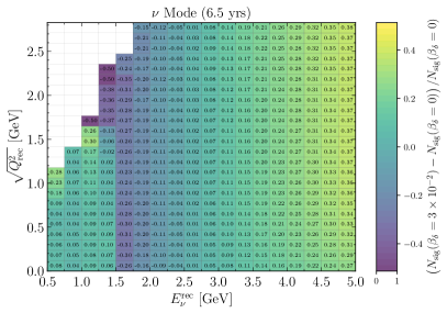
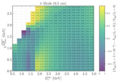
Fig. 9: The relative difference, $\Delta N/N\equiv\left(N_{\rm sig}(\beta_{\delta}=3\times 10^{-2})-N_{\rm sig}(\beta_{\delta}=0)\right)/N_{\rm sig}(\beta_{\delta}=0)$, between the two cases with and without the RG running effect in the two-dimensional $E_{\nu}^{\rm rec}$ and $\sqrt{Q^{2}_{\rm rec}}$ bins for the neutrino (left) and anti-neutrino (right) modes. We take $\delta_{D}=0^{\circ}$ and a 6.5 years of running time for each mode.

To quantify the impact on the CP phase sensitivity from the RG running effect at DUNE, we extend the $\chi^{2}$ function,

$$\chi^{2}=\chi^{2}_{\rm stat}+\chi^{2}_{\rm sys}+\chi^{2}_{\rm prior},$$ (4.9)

by incorporating multiple glb profiles. More concretely, the first term $\chi^{2}_{\rm stat}$ for statistical fluctuations,

$$\chi^{2}_{\rm stat}=\sum_{i^{\prime}j^{\prime}r}\left(\frac{N_{i^{\prime}j^{\prime}}^{r}({\rm true})-(1+a_{r})N_{i^{\prime}j^{\prime}}^{r,{\rm sig}}({\rm test})-(1+b_{r})N_{i^{\prime}j^{\prime}}^{r,{\rm bkg}}({\rm test})}{\sqrt{N_{i^{\prime}j^{\prime}}^{r}({\rm true})}}\right)^{2},\quad$$ (4.10)

needs to sum over not just the two indices $i^{\prime}$ and $j^{\prime}$ for the neutrino energy and the momentum transfer but also the third index $r$ for the various rules from each experimental profile. The quantity $N_{i^{\prime}j^{\prime}}^{r,{\rm sig}}$ ($N_{i^{\prime}j^{\prime}}^{r,{\rm bkg}}$) is the signal (background) event number within the $i^{\prime}$-th reconstructed energy as well as the $j^{\prime}$-th reconstructed momentum transfer bin for the rule $r$ and can be calculated with true or test oscillation parameters. We define $N_{i^{\prime}j^{\prime}}^{r}({\rm true})\equiv N_{i^{\prime}j^{\prime}}^{r,{\rm sig}}({\rm true})+N_{i^{\prime}j^{\prime}}^{r,{\rm bkg}}({\rm true})$ to represent the total event numbers of signal and background with the true oscillation parameters. Moreover, $a_{r}$ and $b_{r}$ are the signal and background normalization nuisance parameters, respectively, for the rule $r$.

The $\chi^{2}_{\rm sys}$ term contains the Gaussian priors of signal and background normalizations. For the signal normalization, we take $\sigma_{\nu_{e},\bar{\nu}_{e}}=2\%$ and $\sigma_{\nu_{\mu},\bar{\nu}_{\mu}}=5\%$ for the electron (anti-)neutrino and muon (anti-)neutrino detection, respectively. A common $5\%$ uncertainty is used for the background normalization. These parameters are taken from the experiment simulation configurations of the DUNE Technical Design Report [91].

The final term $\chi^{2}_{\rm prior}$ summarizes the prior knowledge on the oscillation parameters. We take their best-fit values from the global fit result [42],

$$\sin^{2}\theta_{s}=0.318,\qquad\sin^{2}\theta_{a}=0.574,\qquad\sin^{2}\theta_{r}=0.022,$$ (4.11a)

$$\Delta m^{2}_{s}=7.50\times 10^{-5}\,\mbox{eV}^{2},\qquad\Delta m^{2}_{a}=2.55\times 10^{-3}\,\mbox{eV}^{2}.$$ (4.11b)

Among these oscillation parameters, the solar mass squared difference $\Delta m_{s}^{2}$ and the solar mixing angle $\theta_{s}$ are fixed in our fit since the oscillation probability variation induced by these two parameters is negligibly small [36]. This feature still applies even in the presence of the RG running effect as we have checked numerically. The reactor mixing angle $\theta_{r}$, the atmospheric mixing angle $\theta_{a}$, and the atmospheric mass-squared difference $\Delta m^{2}_{a}$ are treated as free parameters with priors taken from the marginalized one-dimensional $\chi^{2}$ curves [42]. Due to large uncertainties and the existing tension between the T2K and NO$\nu$A results as mentioned in Sec. 1, we do not include any prior on the Dirac CP phase $\delta_{D}$ and simply treat it as a free parameter. Moreover, we take the normal ordering of neutrino masses throughout our study. We first consider a free $\beta_{\delta}$ while the prior knowledge can be extracted from the SBL experiments as we study in Sec. 5.

We perform the $\chi^{2}$ analysis according to Eq. (4.9) to calculate the DUNE sensitivities to $\delta_{D}$ and $\beta_{\delta}$ as shown in the left panel of Fig. 10. Based on the true oscillation parameter setup ($\delta_{D}=270^{\circ}$ and $\beta_{\delta}=0$) that is marked by a black star, the black contours show the sensitivities at confidence levels of $68\%$ (solid), $90\%$ (dashed), $95\%$ (dot-dashed), and $99\%$ (dotted). Those points on the same contour have exactly the same $\Delta\chi^{2}$ value and hence degenerate with each other. Since a positive (negative) $\beta_{\delta}$ can increase (decrease) $\delta_{\rm D}$ according to Eq. (2.2), the combination of a positive $\beta_{\delta}$ and a smaller $\delta_{D}$ degenerates with a combination of opposite values. This degeneracy correlates the two parameters and makes the sensitivity contours tilt from top left (larger $\beta_{\delta}$ and smaller $\delta_{D}$) to bottom right (smaller $\beta_{\delta}$ and larger $\delta_{D}$). The tilting behavior implies that the CP phase sensitivity would be reduced from the case without RG running. Moreover, there is an asymmetry in the sensitivity contour around the black star. The asymmetry is not caused by the RG running effect since it already exists between the intersection points of the contours and the horizontal line for $\beta^{\rm test}_{\delta}=0$. In fact, it arises from the matter effect while the RG running case inherits and enlarges this asymmetry which can also been seen from the right panel.

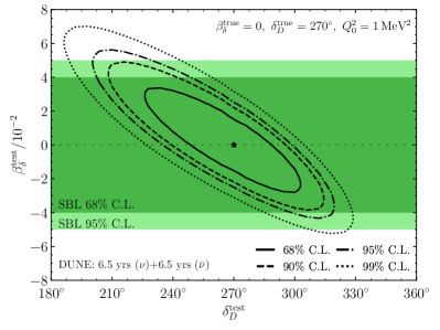
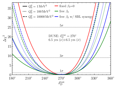
Fig. 10: Left: The two-dimensional sensitivities on $\delta_{D}$ and $\beta_{\delta}$ at the confidence levels of $68\%$ (solid), $90\%$ (dashed), $95\%$ (dot-dashed), and $99\%$ (dotted) with $Q^{2}_{0}=1\,$MeV² and a 6.5 years running time each for the neutrino and anti-neutrino modes. The true parameter setup $\delta^{\rm true}_{D}=270^{\circ}$ and $\beta^{\rm true}_{\delta}=0$ is marked by a black star. Moreover, the SBL $\beta_{\delta}$ constraint at 68% (95%) confidence level is shown by the dark-green (light-green) bands. Right: The marginalized sensitivity to the genuine CP phase $\delta_{D}$ with three different prior cases: the fixed $\beta^{\rm test}_{\delta}=0$ (red), a totally free $\beta^{\rm test}_{\delta}$ (green), and a free $\beta^{\rm test}_{\delta}$ but with the SBL constraint (blue). For comparison, results with $Q^{2}_{0}=1/100/10000\,$MeV² are shown as solid/dotted/dashed curves.

To clearly see the impact of RG running on the CP phase sensitivity, the marginalized $\Delta\chi^{2}$ is shown in the right panel of Fig. 10. The red curve with a fixed $\beta_{\delta}^{\rm test}=0$ corresponds to the standard oscillation case without RG running while the green one sets $\beta_{\delta}^{\rm test}$ free. From the red to the green curves, the CP phase sensitivity significantly reduces. The original $1\sigma$ interval of $\sim[255^{\circ},283^{\circ}]$ changes to $\sim[240^{\circ},295^{\circ}]$ with almost a factor of 2 reduction.

Moreover, we investigate the effect of the reference momentum transfer $Q^{2}_{0}$ by considering three different values: $Q^{2}_{0}=1\,$MeV² (solid), 100 MeV² (dotted), and 10000 MeV² (dashed). Although the CP phase sensitivity increases with $Q^{2}_{0}$ since the distance from the actual momentum transfer $Q^{2}_{d}$ decreases to reduce the RG running effect, the impact on the CP measurement at DUNE still cannot be neglected even for $Q^{2}_{0}=10000\,$MeV². Therefore, there exists a large parameter space for the energy scale of new physics that can significantly affect the leptonic CP phase sensitivity.

5 Synergy with Existing Short-Baseline Experiments

In the zero-distance limit, the probability of flavor transition induced by the RG running effect depends on the CP phase difference $\Delta\delta_{D}$ instead of the genuine CP phase $\delta_{D}$ as shown in Eq. (3.13). Hence SBL experiments can provide a clean measurement for RG running. Therefore, a synergy between the long- and short-baseline experiments can disentangle the genuine CP phase ($\delta_{D}$) from the RG running effect ($\beta_{\delta}$).

The searches for neutrino transition in the zero-distance limit are done by $\mathcal{O}(100\,\rm{m})$ SBL experiments such as ICARUS [92], CHARM-II [93], NOMAD [94], and NuTeV [95]. All these four experiments use both $\nu_{\mu}$ and $\nu_{e}$ neutrinos as well as the anti-neutrino counterparts. Since ICARUS has only 4 detected $\nu_{e}$ events from the result [92], we will not take it into account due to lack of statistical significance. As for the other three (CHARM-II, NOMAD, and NuTeV), $\mathcal{O}(1000)$ $\nu_{e}$ events are detected at each experiment [93, 94, 95]. Note that anti-neutrinos are also detected at CHARM-II and NuTeV. Since the anti-neutrino case is similar to the neutrino one, we just discuss the neutrino case at SBL experiments for illustration in the following text. These $\nu_{e}$ neutrinos are from two sources: the $\nu_{e}$ disappearance from the $\nu_{e}$ flux and those from the $\nu_{\mu}\rightarrow\nu_{e}$ transition due to the zero-distance effect. The experimental constraint on the $\nu_{\mu}\rightarrow\nu_{e}$ transition probability can be obtained by comparing the predicted $\nu_{e}$ neutrino spectra with the experimental data. Besides the $\nu_{\mu}\rightarrow\nu_{e}$ transition, these SBL experiments can also search for $\nu_{e}\rightarrow\nu_{\tau}$ as well as $\nu_{\mu}\rightarrow\nu_{\tau}$ [96, 97, 98]. However, since the charged $\tau$ lepton produced from $\nu_{\tau}$ CC scattering decays immediately into final-state particles such as $e$, $\mu$, $\pi$, and $K$ that can also be produced in other CC or NC events, the detection of $\nu_{\tau}$ suffers from these potential backgrounds. Moreover, the $\tau$ selection criteria include much more kinematic requirements than its counterparts of $e$, which needs more complicated analysis. The SBL experiments find no evidence of $\nu_{\tau}$ with large background uncertainties. Hence we do not consider such $\nu_{e,\mu}\rightarrow\nu_{\tau}$ transition channels in our current study.

To obtain the experimental constraint on $\beta_{\delta}$, we first calculate the predicted $\nu_{e}$ event rate with the RG running effect. For a neutrino experiment, the predicted $\nu_{e}$ event rate can be described as $N_{\nu_{e}}=A\sum_{\alpha}\phi(\nu_{\alpha})P_{\alpha e}\sigma(\nu_{e})$ with $A$ being the coefficient that is related to the experimental efficiencies and reconstruction errors of the detector, $\phi(\nu_{\alpha})$ the $\alpha$ flavor neutrino flux, $P_{\alpha e}$ the $\nu_{\alpha}\rightarrow\nu_{e}$ oscillation probability, and $\sigma(\nu_{e})$ the cross section for scattering between $\nu_{e}$ and target. The predicted $\nu_{e}$ event rate $R(\nu_{e})$ from the collaboration [93, 94, 95] was obtained by assuming no oscillation, $P_{\alpha e}=\delta_{\alpha e}$. As for the case with RG running, we calculate the predicted $\nu_{e}$ event rates $R^{\prime}(\nu_{e})$ by multiplying the transition probability in Eq. (3.13) with the $\nu_{e}$ and $\nu_{\mu}$ MC neutrino event rates ($R(\nu_{e})$ and $R(\nu_{\mu})$), $R^{\prime}(\nu_{e})\equiv P_{\nu_{e}\rightarrow\nu_{e}}R(\nu_{e})+P_{\nu_{\mu}\rightarrow\nu_{e}}R(\nu_{\mu})$. We take $\sigma(\nu_{e})\approx\sigma(\nu_{\mu})$ since the neutrino energy is much larger than the charged lepton masses.

Note that the transition probabilities $P_{\nu_{e}\rightarrow\nu_{e}}$ and $P_{\nu_{\mu}\rightarrow\nu_{e}}$ with the RG running effect are $Q^{2}_{d}$ dependent as discussed in Sec. 3. So the typical high-energy neutrinos at SBL experiments have the advantage of producing large momentum transfer to enhance the RG running effect. However, there is no such momentum transfer information in the published SBL experimental data [93, 94, 95]. So in the transition probability calculation, we take the averaged oscillation probability by integrating Eq. (3.13) over the $Q^{2}_{d}$ distribution extracted from the GENIE simulation.

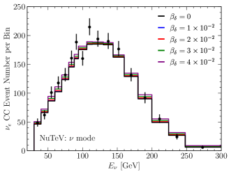
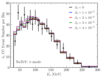
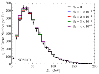
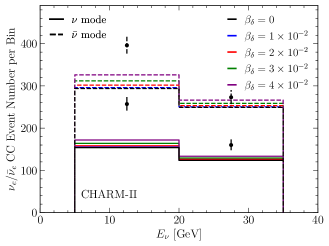
Fig. 11: The $\nu_{e}/\bar{\nu}_{e}$ CC event rates for NuTeV with the neutrino mode (upper left), NuTeV with the anti-neutrino mode (upper right), NOMAD with the neutrino mode (lower left), and CHARM-II with both modes (lower right), respectively. Besides the data points (black dot with error bar), the RG running effect is shown with $\beta_{\delta}=0$ (black), $1\times 10^{-2}$ (blue), $2\times 10^{-2}$ (red), $3\times 10^{-2}$ (green), and $4\times 10^{-2}$ (purple).

Fig. 11 shows the predicted electron-flavor neutrino event rates as well as the experimental data from NuTeV, NOMAD, and CHARM-II. For all experiments, the predicted event rates with a percentage level $\beta_{\delta}$ are roughly $\mathcal{O}(10\%)$ more than the MC prediction without flavor transition. Note that flipping the sign of $\beta_{\delta}$ does not affect the predicted event rates since $\beta_{\delta}$ only appears as the squared term $\sin^{2}(\Delta\delta_{D}/2)$ in Eq. (3.13). Such variations are comparable with the experimental uncertainties which means the experimental sensitivity to $\beta_{\delta}$ can reach percentage level. Moreover, with the predicted event rates being a linear combination of both the $\nu_{e}$ MC neutrino event rate $R(\nu_{e})$ and the $\nu_{\mu}$ counterpart $R(\nu_{\mu})$, the largest variation between the predicted and expected event rates does not exactly occur at the $\nu_{e}$ event rate peak position since the $\nu_{e}$ and $\nu_{\mu}$ fluxes peak at different energies [93, 94, 95].

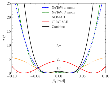
Fig. 12: The $\Delta\chi^{2}$ ($\equiv\chi^{2}-\chi^{2}_{\rm min}$) as a function of $\beta_{\delta}$ for NuTeV with the neutrino mode (dashed blue), NuTeV with the anti-neutrino mode (dot-dashed green), NOMAD with the neutrino mode (dotted orange), CHARM-II with both neutrino and anti-neutrino modes (solid red), and their combination (solid black). Moreover, the $1\sigma$, $2\sigma$, and $3\sigma$ confidence levels are shown by horizontal black dotted lines.

To obtain the sensitivity on $\beta_{\delta}$, we consider the following $\chi^{2}$ function,

$$\chi^{2}\equiv \sum_{i=1}^{n_{\rm bins}}\left(\frac{N^{{\rm data},i}-(1+b^{e})N^{{\rm fit},i}_{\nu_{e}\rightarrow\nu_{e}}-(1+b^{\mu})N^{{\rm fit},i}_{\nu_{\mu}\rightarrow\nu_{e}}}{\sqrt{N^{{\rm data},i}+(N^{{\rm fit},i}_{\nu_{e}\rightarrow\nu_{e}}\sigma_{i}^{e})^{2}+(N^{{\rm fit},i}_{\nu_{\mu}\rightarrow\nu_{e}}\sigma_{i}^{\mu})^{2}}}\right)^{2}+\left(\frac{b^{e}}{\sigma_{e}}\right)^{2}+\left(\frac{b^{\mu}}{\sigma_{\mu}}\right)^{2},$$ (5.1)

where $N^{{\rm data},i}$ and $N^{{\rm fit},i}_{\nu_{\alpha}\rightarrow\nu_{e}}$ are the experimental data and predicted event number in the $i$-th energy bin, respectively. The nuisance parameter $b^{e}$ ($b^{\mu}$) describes the total normalization uncertainty $\sigma_{e}$ ($\sigma_{\mu}$) for the electron-flavor (muon-flavor) neutrino flux. Moreover, the parameters $\sigma_{i}^{e}$ and $\sigma_{i}^{\mu}$ are the systematic uncertainties in each energy bin [93, 99, 95]. We obtain the constraint on $\beta_{\delta}$ by minimizing $\chi^{2}$ over the nuisance parameters and subtracting the global minimum value $\chi^{2}_{\rm min}$, $\Delta\chi^{2}\equiv\chi^{2}-\chi^{2}_{\rm min}$, as shown in Fig. 12. For NuTeV with both $\nu$ (dashed blue) and $\bar{\nu}$ modes (dot-dashed green), the $\Delta\chi^{2}$ curve is flat in the region of $|\beta_{\delta}|\lesssim 4\times 10^{-2}$, but raises quickly at larger values. The NOMAD experiment (dotted orange) is more sensitive to smaller $|\beta_{\delta}|$ than NuTeV with higher statistics. For NOMAD and the $\nu$ mode at NuTeV, the $\Delta\chi^{2}$ minimum lies at $\beta_{\delta}=0$, while the $\bar{\nu}$ mode at NuTeV slightly prefers a non-zero $\beta_{\delta}$. Moreover, the CHARM-II experiment (solid red) disfavors $\beta_{\delta}=0$ by $\sim 2\sigma$ since the observed data points have an excess over the expected event rates as shown in Fig. 11. Note that all these $\Delta\chi^{2}$ curves are symmetric around $\beta_{\delta}=0$ since the predicted event rates do not depend on the sign of $\beta_{\delta}$ as explained before. The combined result (solid black) of these experiments gives a bound of $|\beta_{\delta}|\lesssim 4\times 10^{-2}$ ($5\times 10^{-2}$) at $68\%$ ($95\%$) confidence level with the best fit being $|\beta_{\delta}|\approx 2.5\times 10^{-2}$.

For comparison, we show the 68% and 95% sensitivities on $\beta_{\delta}$ as dark- and light-green bands in the left panel of Fig. 10. Since the $\beta_{\delta}$ sensitivities at SBL experiments is actually comparable with the one at DUNE, their synergy should further improve the sensitivity. As the SBL experiments (NuTeV, NOMAD, and CHARM-II) already have existing data, their constraints on $\beta_{\delta}$ can be treated as priors. The $\Delta\chi^{2}$ curves shown in the right panel of Fig. 10 does improve after taking the SBL priors into consideration. Note that the current priors at SBL experiments are obtained without considering the momentum transfer distribution due to lack of information. A more detailed analysis with full data from the experimental side should significantly enhance the existing priors.

6 Conclusion & Discussion

We establish a general and complete formalism for studying the RG running effect on the neutrino oscillation. Especially, our formalism allows an energy dependent momentum transfer for the forward scattering and hence the matter potential. With a broad momentum transfer distribution instead of a single fixed value, our study shows that the degeneracy between the RG running parameter $\beta_{\delta}$ and the genuine CP phase $\delta_{D}$ will significantly reduce the CP phase sensitivity at DUNE. With mismatch between the momentum transfers in the neutrino production and detection processes, the transition probability of the appearance channels does not vanish even in the limit of zero distance. Consequently, the short-baseline experiments can provide an independent measurement of the RG running parameter $\beta_{\delta}$ and its synergy with the long-baseline DUNE can help to disentangle the degeneracy and restore the CP phase sensitivity to some extent. Due to lack of information on the momentum transfer, the $\beta_{\delta}$ sensitivity at short-baseline experiments (NuTeV, NOMAD, and CHARM-II) is comparable with the one at DUNE. We expect more disentangling capability with full data and detailed analysis from the experimental side.

References

- [1] L. Canetti, M. Drewes and M. Shaposhnikov, “Matter and Antimatter in the Universe,” New J. Phys. 14, 095012 (2012) [arXiv:1204.4186 [hep-ph]].
- [2] A. D. Sakharov, “Violation of CP Invariance, C asymmetry, and baryon asymmetry of the universe,” Pisma Zh. Eksp. Teor. Fiz. 5, 32-35 (1967)
- [3] M. B. Gavela, P. Hernandez, J. Orloff and O. Pene, “Standard model CP violation and baryon asymmetry,” Mod. Phys. Lett. A 9, 795-810 (1994) [arXiv:hep-ph/9312215 [hep-ph]].
- [4] P. Huet and E. Sather, “Electroweak baryogenesis and standard model CP violation,” Phys. Rev. D 51, 379-394 (1995) [arXiv:hep-ph/9404302 [hep-ph]].
- [5] M. B. Gavela, P. Hernandez, J. Orloff, O. Pene and C. Quimbay, “Standard model CP violation and baryon asymmetry. Part 2: Finite temperature,” Nucl. Phys. B 430, 382-426 (1994) [arXiv:hep-ph/9406289 [hep-ph]].
- [6] M. Fukugita and T. Yanagida, “Baryogenesis Without Grand Unification,” Phys. Lett. B 174, 45-47 (1986).
- [7] W. Buchmuller, R. D. Peccei and T. Yanagida, “Leptogenesis as the origin of matter,” Ann. Rev. Nucl. Part. Sci. 55, 311-355 (2005) [arXiv:hep-ph/0502169 [hep-ph]].
- [8] S. Davidson, E. Nardi and Y. Nir, “Leptogenesis,” Phys. Rept. 466, 105-177 (2008) [arXiv:0802.2962 [hep-ph]].
- [9] M. C. Gonzalez-Garcia and M. Yokoyam, “Neutrino Masses, Mixing, and Oscillations”, (Chapter 14) of R. L. Workman et al. [Particle Data Group], “Review of Particle Physics,” PTEP 2022, 083C01 (2022).
- [10] S. Pascoli, S. T. Petcov and A. Riotto, “Connecting low energy leptonic CP-violation to leptogenesis,” Phys. Rev. D 75, 083511 (2007) [arXiv:hep-ph/0609125 [hep-ph]].
- [11] G. C. Branco, R. Gonzalez Felipe and F. R. Joaquim, “A New bridge between leptonic CP violation and leptogenesis,” Phys. Lett. B 645, 432-436 (2007) [arXiv:hep-ph/0609297 [hep-ph]].
- [12] S. Pascoli, S. T. Petcov and A. Riotto, “Leptogenesis and Low Energy CP Violation in Neutrino Physics,” Nucl. Phys. B 774, 1-52 (2007) [arXiv:hep-ph/0611338 [hep-ph]].
- [13] A. Anisimov, S. Blanchet and P. Di Bari, “Viability of Dirac phase leptogenesis,” JCAP 04, 033 (2008) [arXiv:0707.3024 [hep-ph]].
- [14] E. Molinaro and S. T. Petcov, “The Interplay Between the ’Low’ and ’High’ Energy CP-Violation in Leptogenesis,” Eur. Phys. J. C 61, 93-109 (2009) [arXiv:0803.4120 [hep-ph]].
- [15] Shao-Feng Ge, Hong-Jian He and Fu-Rong Yin, “Common Origin of Soft mu-tau and CP Breaking in Neutrino Seesaw and the Origin of Matter,” JCAP 05, 017 (2010) [arXiv:1001.0940 [hep-ph]].
- [16] M. J. Dolan, T. P. Dutka and R. R. Volkas, “Dirac-Phase Thermal Leptogenesis in the extended Type-I Seesaw Model,” JCAP 06, 012 (2018) [arXiv:1802.08373 [hep-ph]].
- [17] M. A. Acero et al. [NOvA], “First Measurement of Neutrino Oscillation Parameters using Neutrinos and Antineutrinos by NOvA,” Phys. Rev. Lett. 123, no.15, 151803 (2019) [arXiv:1906.04907 [hep-ex]].
- [18] K. Abe et al. [T2K], “Constraint on the matter–antimatter symmetry-violating phase in neutrino oscillations,” Nature 580, no.7803, 339-344 (2020) [erratum: Nature 583, no.7814, E16 (2020)] [arXiv:1910.03887 [hep-ex]].
- [19] D. S. Ayres et al. [NOvA], “NOvA: Proposal to Build a 30 Kiloton Off-Axis Detector to Study Oscillations in the NuMI Beamline,” [arXiv:hep-ex/0503053 [hep-ex]].
- [20] K. Abe et al. [T2K], “The T2K Experiment,” Nucl. Instrum. Meth. A 659, 106-135 (2011) [arXiv:1106.1238 [physics.ins-det]].
- [21] M. A. Acero et al. [NOvA and R. Group], “An Improved Measurement of Neutrino Oscillation Parameters by the NOA Experiment,” [arXiv:2108.08219 [hep-ex]].
- [22] M. A. Ramírez et al. [T2K], “Measurements of neutrino oscillation parameters from the T2K experiment using protons on target,” [arXiv:2303.03222 [hep-ex]].
- [23] R. Acciarri et al. [DUNE], “Long-Baseline Neutrino Facility (LBNF) and Deep Underground Neutrino Experiment (DUNE): Conceptual Design Report, Volume 2: The Physics Program for DUNE at LBNF,” [arXiv:1512.06148 [physics.ins-det]].
- [24] K. Abe, T. Abe, H. Aihara, Y. Fukuda, Y. Hayato, K. Huang, A. K. Ichikawa, M. Ikeda, K. Inoue and H. Ishino, et al. “Letter of Intent: The Hyper-Kamiokande Experiment — Detector Design and Physics Potential —,” [arXiv:1109.3262 [hep-ex]].
- [25] K. Abe et al. [Hyper-Kamiokande], “Hyper-Kamiokande Design Report,” [arXiv:1805.04163 [physics.ins-det]].
- [26] A. Abud Abed et al. [DUNE], “Low exposure long-baseline neutrino oscillation sensitivity of the DUNE experiment,” Phys. Rev. D 105, no.7, 072006 (2022) [arXiv:2109.01304 [hep-ex]].
- [27] A. Alekou et al. [ESSnuSB], “Updated physics performance of the ESSnuSB experiment: ESSnuSB collaboration,” Eur. Phys. J. C 81, no.12, 1130 (2021) [arXiv:2107.07585 [hep-ex]].
- [28] K. Abe et al. [Hyper-Kamiokande], “Physics potentials with the second Hyper-Kamiokande detector in Korea,” PTEP 2018, no.6, 063C01 (2018) [arXiv:1611.06118 [hep-ex]].
- [29] J. Tang, S. Vihonen and T. C. Wang, “Precision measurements on in MOMENT,” JHEP 12, 130 (2019) [arXiv:1909.01548 [hep-ph]].
- [30] A. V. Akindinov, E. G. Anassontzis, G. Anton, M. Ardid, J. Aublin, B. Baret, V. Bertin, S. Bourret, C. Bozza and M. Bruchner, et al. “Letter of Interest for a Neutrino Beam from Protvino to KM3NeT/ORCA,” Eur. Phys. J. C 79, no.9, 758 (2019) [arXiv:1902.06083 [physics.ins-det]].
- [31] J. Alonso, F. T. Avignone, W. A. Barletta, R. Barlow, H. T. Baumgartner, A. Bernstein, E. Blucher, L. Bugel, L. Calabretta and L. Camilleri, et al. “Expression of Interest for a Novel Search for CP Violation in the Neutrino Sector: DAEdALUS,” [arXiv:1006.0260 [physics.ins-det]].
- [32] E. Ciuffoli, J. Evslin and X. Zhang, “The Leptonic CP Phase from Muon Decay at Rest with Two Detectors,” JHEP 12, 051 (2014) [ arXiv:1401.3977 [hep-ph]].
- [33] E. Ciuffoli, J. Evslin and F. Zhao, “Neutrino Physics with Accelerator Driven Subcritical Reactors,” JHEP 01, 004 (2016) [arXiv:1509.03494 [hep-ph]].
- [34] Jarah Evslin, Shao-Feng Ge and Kaoru Hagiwara, “The leptonic CP phase from T2(H)K and + decay at rest,” JHEP 02, 137 (2016) [arXiv:1506.05023 [hep-ph]]; Shao-Feng Ge “Measuring the Leptonic Dirac CP Phase with TNT2K,” [arXiv:1704.08518 [hep-ph]] at NuPhys2016: Prospects in Neutrino Physics, Barbican Centre, London, UK, December 12-14, 2016;
- [35] M. V. Smirnov, Z. J. Hu, S. J. Li and J. J. Ling, “The possibility of leptonic CP-violation measurement with JUNO,” Nucl. Phys. B 931, 437-445 (2018) [arXiv:1802.03677 [hep-ph]].
- [36] Shao-Feng Ge, Chui-Fan Kong and Pedro Pasquini, “Improving CP measurement with THEIA and muon decay at rest,” Eur. Phys. J. C 82, no.6, 572 (2022) [arXiv:2202.05038 [hep-ph]].
- [37] S. Razzaque and A. Y. Smirnov, “Super-PINGU for measurement of the leptonic CP-phase with atmospheric neutrinos,” JHEP 05, 139 (2015) [arXiv:1406.1407 [hep-ph]].
- [38] S. Razzaque and A. Y. Smirnov, “Super-PINGU for measuring CP violation,” Nucl. Part. Phys. Proc. 265-266, 183-185 (2015) [arXiv:1501.03145 [hep-ph]].
- [39] J. Hofestädt, M. Bruchner and T. Eberl, “Super-ORCA: Measuring the leptonic CP-phase with Atmospheric Neutrinos and Beam Neutrinos,” PoS ICRC2019, 911 (2020) [arXiv:1907.12983 [hep-ex]].
- [40] F. An et al. [JUNO], “Neutrino Physics with JUNO,” J. Phys. G 43, no.3, 030401 (2016) [arXiv:1507.05613 [physics.ins-det]].
- [41] K. J. Kelly, P. A. Machado, I. Martinez Soler, S. J. Parke and Y. F. Perez Gonzalez, “Sub-GeV Atmospheric Neutrinos and CP-Violation in DUNE,” Phys. Rev. Lett. 123, no.8, 081801 (2019) [arXiv:1904.02751 [hep-ph]].
- [42] P. F. de Salas, D. V. Forero, S. Gariazzo, P. Martínez-Miravé, O. Mena, C. A. Ternes, M. Tórtola and J. W. F. Valle, “2020 global reassessment of the neutrino oscillation picture,” JHEP 02 (2021), 071 [arXiv:2006.11237 [hep-ph]]. See tables in the Valencia neutrino global fit.
- [43] M. C. Gonzalez-Garcia, M. Maltoni and T. Schwetz, “NuFIT: Three-Flavour Global Analyses of Neutrino Oscillation Experiments,” Universe 7 (2021) no.12, 459 [arXiv:2111.03086 [hep-ph]].
- [44] V. De Romeri, E. Fernandez-Martinez and M. Sorel, “Neutrino oscillations at DUNE with improved energy reconstruction,” JHEP 09 (2016), 030 [arXiv:1607.00293 [hep-ph]].
- [45] S. K. Raut, “Matter effects at the T2HK and T2HKK experiments,” Phys. Rev. D 96 (2017) no.7, 075029 [arXiv:1703.07136 [hep-ph]].
- [46] K. J. Kelly and S. J. Parke, “Matter Density Profile Shape Effects at DUNE,” Phys. Rev. D 98 (2018) no.1, 015025 [arXiv:1802.06784 [hep-ph]].
- [47] S. F. King, S. Molina Sedgwick, S. J. Parke and N. W. Prouse, “Effects of matter density profiles on neutrino oscillations for T2HK and T2HKK,” Phys. Rev. D 101 (2020), 076019 [arXiv:2001.05505 [hep-ph]].
- [48] Y. Farzan and M. Tortola, “Neutrino oscillations and Non-Standard Interactions,” Front. in Phys. 6, 10 (2018) [arXiv:1710.09360 [hep-ph]].
- [49] P. S. Bhupal Dev, K. S. Babu, P. B. Denton, P. A. N. Machado, C. A. Argüelles, J. L. Barrow, S. S. Chatterjee, M. C. Chen, A. de Gouvêa and B. Dutta, et al. “Neutrino Non-Standard Interactions: A Status Report,” SciPost Phys. Proc. 2, 001 (2019) [arXiv:1907.00991 [hep-ph]].
- [50] Shao-Feng Ge and Alexei Y. Smirnov, “Non-standard interactions and the CP phase measurements in neutrino oscillations at low energies,” JHEP 10, 138 (2016) [arXiv:1607.08513 [hep-ph]].
- [51] Shao-Feng Ge, “The Leptonic CP Measurement and New Physics Alternatives” PoS NuFact2019 (2020) 108 at The 21st International Workshop on Neutrinos from Accelerators (NUFACT2019), Daegu, Korea, August 29, 2019; “New Physics with Scalar and Dark Non-Standard Interactions in Neutrino Oscillation” J.Phys.Conf.Ser. 1468 (2020) 1, 012125 at The 16th International Conference on Topics in Astroparticle and Underground Physics, Toyama, Japan, September 10, 2019.
- [52] P. Bakhti and M. Rajaee, “Sensitivities of future reactor and long-baseline neutrino experiments to NSI,” Phys. Rev. D 103, no.7, 075003 (2021) [arXiv:2010.12849 [hep-ph]].
- [53] S. S. Chatterjee, P. S. B. Dev and P. A. N. Machado, “Impact of improved energy resolution on DUNE sensitivity to neutrino non-standard interactions,” JHEP 08, 163 (2021) [arXiv:2106.04597 [hep-ph]].
- [54] A. Medhi, D. Dutta and M. M. Devi, “Exploring the effects of scalar non standard interactions on the CP violation sensitivity at DUNE,” JHEP 06, 129 (2022) [arXiv:2111.12943 [hep-ph]].
- [55] A. Medhi, M. M. Devi and D. Dutta, “Imprints of scalar NSI on the CP-violation sensitivity using synergy among DUNE, T2HK and T2HKK,” JHEP 01, 079 (2023) [arXiv:2209.05287 [hep-ph]].
- [56] J. S. Diaz, “Neutrinos as probes of Lorentz invariance,” Adv. High Energy Phys. 2014, 962410 (2014) [arXiv:1406.6838 [hep-ph]].
- [57] M. D. C. Torri, “Neutrino Oscillations and Lorentz Invariance Violation,” Universe 6, no.3, 37 (2020) [arXiv:2110.09186 [hep-ph]].
- [58] H. X. Lin, J. Tang, S. Vihonen and P. Pasquini, “Nonminimal Lorentz invariance violation in light of the muon anomalous magnetic moment and long-baseline neutrino oscillation data,” Phys. Rev. D 105 (2022) no.9, 096029 [arXiv:2111.14336 [hep-ph]].
- [59] R. Majhi, S. Chembra and R. Mohanta, “Exploring the effect of Lorentz invariance violation with the currently running long-baseline experiments,” Eur. Phys. J. C 80, no.5, 364 (2020) [arXiv:1907.09145 [hep-ph]].
- [60] S. Kumar Agarwalla and M. Masud, “Can Lorentz invariance violation affect the sensitivity of deep underground neutrino experiment?,” Eur. Phys. J. C 80, no.8, 716 (2020) [arXiv:1912.13306 [hep-ph]].
- [61] N. Fiza, N. R. Khan Chowdhury and M. Masud, “Investigating Lorentz Invariance Violation with the long baseline experiment P2O,” JHEP 01, 076 (2023) [arXiv:2206.14018 [hep-ph]].
- [62] D. V. Forero, S. Morisi, M. Tortola and J. W. F. Valle, “Lepton flavor violation and non-unitary lepton mixing in low-scale type-I seesaw,” JHEP 09, 142 (2011) [arXiv:1107.6009 [hep-ph]].
- [63] F. J. Escrihuela, D. V. Forero, O. G. Miranda, M. Tortola and J. W. F. Valle, “On the description of nonunitary neutrino mixing,” Phys. Rev. D 92, no.5, 053009 (2015) [erratum: Phys. Rev. D 93, no.11, 119905 (2016)] [arXiv:1503.08879 [hep-ph]].
- [64] Shao-Feng Ge, Pedro Pasquini, M. Tortola and J. W. F. Valle, “Measuring the leptonic CP phase in neutrino oscillations with nonunitary mixing,” Phys. Rev. D 95, no.3, 033005 (2017) [arXiv:1605.01670 [hep-ph]].
- [65] P. Pasquini, S. F. Ge, M. A. Tórtola and J. W. F. Valle, “Measuring the Leptonic CP Phase in Neutrino Oscillations with Non-Unitary Mixing,” PoS NOW2016, 026 (2017) at the Neutrino Oscillation Workshop (NOW) 2016, Otranto, Lecce, Italy, September 4-11, 2016.
- [66] F. J. Escrihuela, D. V. Forero, O. G. Miranda, M. Tórtola and J. W. F. Valle, “Probing CP violation with non-unitary mixing in long-baseline neutrino oscillation experiments: DUNE as a case study,” New J. Phys. 19, no.9, 093005 (2017) [arXiv:1612.07377 [hep-ph]].
- [67] D. V. Forero, C. Giunti, C. A. Ternes and M. Tortola, “Nonunitary neutrino mixing in short and long-baseline experiments,” Phys. Rev. D 104, no.7, 075030 (2021) [arXiv:2103.01998 [hep-ph]].
- [68] I. Martinez-Soler and H. Minakata, “Standard versus Non-Standard CP Phases in Neutrino Oscillation in Matter with Non-Unitarity,” PTEP 2020, no.6, 063B01 (2020) [arXiv:1806.10152 [hep-ph]].
- [69] J. Huang and S. Zhou, “The Mikheyev-Smirnov-Wolfenstein Matter Potential at the One-loop Level in the Standard Model,” [arXiv:2307.04685 [hep-ph]].
- [70] J. A. Casas, J. R. Espinosa, A. Ibarra and I. Navarro, “General RG equations for physical neutrino parameters and their phenomenological implications,” Nucl. Phys. B 573, 652-684 (2000) [arXiv:hep-ph/9910420 [hep-ph]].
- [71] P. H. Chankowski and S. Pokorski, “Quantum corrections to neutrino masses and mixing angles,” Int. J. Mod. Phys. A 17, 575-614 (2002) [arXiv:hep-ph/0110249 [hep-ph]].
- [72] S. Antusch, J. Kersten, M. Lindner and M. Ratz, “Running neutrino masses, mixings and CP phases: Analytical results and phenomenological consequences,” Nucl. Phys. B 674, 401-433 (2003) [arXiv:hep-ph/0305273 [hep-ph]].
- [73] S. Ray, “Renormalization group evolution of neutrino masses and mixing in seesaw models: A Review,” Int. J. Mod. Phys. A 25, 4339-4384 (2010) [arXiv:1005.1938 [hep-ph]].
- [74] T. Ohlsson and S. Zhou, “Renormalization group running of neutrino parameters,” Nature Commun. 5 (2014), 5153 [arXiv:1311.3846 [hep-ph]].
- [75] K. S. Babu, V. Brdar, A. de Gouvêa and P. A. N. Machado, “Energy-dependent neutrino mixing parameters at oscillation experiments,” Phys. Rev. D 105, no.11, 115014 (2022) [arXiv:2108.11961 [hep-ph]].
- [76] K. S. Babu, C. N. Leung and J. T. Pantaleone, “Renormalization of the neutrino mass operator,” Phys. Lett. B 319, 191-198 (1993) [arXiv:hep-ph/9309223 [hep-ph]].
- [77] P. H. Chankowski and Z. Pluciennik, “Renormalization group equations for seesaw neutrino masses,” Phys. Lett. B 316 (1993), 312-317 [arXiv:hep-ph/9306333 [hep-ph]].
- [78] W. Grimus and P. Stockinger, “Real oscillations of virtual neutrinos,” Phys. Rev. D 54, 3414-3419 (1996) [arXiv:hep-ph/9603430 [hep-ph]].
- [79] A. Falkowski, M. González-Alonso and Z. Tabrizi, “Consistent QFT description of non-standard neutrino interactions,” JHEP 11 (2020), 048 [arXiv:1910.02971 [hep-ph]].
- [80] C. Giunti, C. W. Kim, J. A. Lee and U. W. Lee, “On the treatment of neutrino oscillations without resort to weak eigenstates,” Phys. Rev. D 48, 4310-4317 (1993) [arXiv:hep-ph/9305276 [hep-ph]].
- [81] M. Beuthe, “Oscillations of neutrinos and mesons in quantum field theory,” Phys. Rept. 375 (2003), 105-218 [arXiv:hep-ph/0109119 [hep-ph]].
- [82] B. Abi et al. [DUNE], “Deep Underground Neutrino Experiment (DUNE), Far Detector Technical Design Report, Volume II: DUNE Physics,” [arXiv:2002.03005 [hep-ex]].
- [83] C. Andreopoulos, A. Bell, D. Bhattacharya, F. Cavanna, J. Dobson, S. Dytman, H. Gallagher, P. Guzowski, R. Hatcher and P. Kehayias, et al. “The GENIE Neutrino Monte Carlo Generator,” Nucl. Instrum. Meth. A 614, 87-104 (2010) [arXiv:0905.2517 [hep-ph]].
- [84] C. Andreopoulos, C. Barry, S. Dytman, H. Gallagher, T. Golan, R. Hatcher, G. Perdue and J. Yarba, “The GENIE Neutrino Monte Carlo Generator: Physics and User Manual,” [arXiv:1510.05494 [hep-ph]].
- [85] A. Friedland and S. W. Li, “Understanding the energy resolution of liquid argon neutrino detectors,” Phys. Rev. D 99, no.3, 036009 (2019) [arXiv:1811.06159 [hep-ph]].
- [86] Shao-Feng Ge and Kaoru Hagiwara, “Physics Reach of Atmospheric Neutrino Measurements at PINGU,” JHEP 09, 024 (2014) [arXiv:1312.0457 [hep-ph]].
- [87] P. Huber, M. Lindner and W. Winter, “Simulation of long-baseline neutrino oscillation experiments with GLoBES (General Long Baseline Experiment Simulator),” Comput. Phys. Commun. 167, 195 (2005) [arXiv:hep-ph/0407333 [hep-ph]].
- [88] P. Huber, J. Kopp, M. Lindner, M. Rolinec and W. Winter, “New features in the simulation of neutrino oscillation experiments with GLoBES 3.0: General Long Baseline Experiment Simulator,” Comput. Phys. Commun. 177, 432-438 (2007) [arXiv:hep-ph/0701187 [hep-ph]].
- [89] W. Winter, “Neutrino mass hierarchy determination with IceCube-PINGU,” Phys. Rev. D 88, no.1, 013013 (2013) [arXiv:1305.5539 [hep-ph]].
- [90] W. Winter, “Atmospheric Neutrino Oscillations for Earth Tomography,” Nucl. Phys. B 908, 250-267 (2016) [arXiv:1511.05154 [hep-ph]].
- [91] B. Abi et al. [DUNE], “Experiment Simulation Configurations Approximating DUNE TDR,” [arXiv:2103.04797 [hep-ex]].
- [92] M. Antonello et al. [ICARUS], “Search for anomalies in the appearance from a beam,” Eur. Phys. J. C 73, 2599 (2013) [arXiv:1307.4699 [hep-ex]].
- [93] P. Vilain et al. [CHARM II], “Search for muon to electron-neutrino oscillations,” Z. Phys. C 64, 539-544 (1994)
- [94] P. Astier et al. [NOMAD], “Search for nu(mu) — nu(e) oscillations in the NOMAD experiment,” Phys. Lett. B 570, 19-31 (2003) [arXiv:hep-ex/0306037 [hep-ex]].
- [95] S. Avvakumov et al. [NuTeV], “A Search for and Oscillations at NuTeV,” Phys. Rev. Lett. 89, 011804 (2002) [arXiv:hep-ex/0203018 [hep-ex]].
- [96] M. Gruwe et al. [CHARM-II], “Search for muon-neutrino — tau-neutrino oscillation,” Phys. Lett. B 309, 463-468 (1993)
- [97] P. Astier et al. [NOMAD], “Final NOMAD results on muon-neutrino — tau-neutrino and electron-neutrino — tau-neutrino oscillations including a new search for tau-neutrino appearance using hadronic tau decays,” Nucl. Phys. B 611, 3-39 (2001) [arXiv:hep-ex/0106102 [hep-ex]].
- [98] D. Naples et al. [CCFR/NuTeV], “A High statistics search for neutrino(e) (anti-neutrino(e)) — neutrino(tau) (anti-neutrino(tau)) oscillations,” Phys. Rev. D 59, 031101 (1999) [arXiv:hep-ex/9809023 [hep-ex]].
- [99] P. Astier et al. [NOMAD], “Prediction of neutrino fluxes in the NOMAD experiment,” Nucl. Instrum. Meth. A 515, 800-828 (2003) [arXiv:hep-ex/0306022 [hep-ex]].