Variational principle for mean dimension with potential of $\mathbb{R}^{d}$-actions: I

Abstract.

We develop a variational principle for mean dimension with potential of $\mathbb{R}^{d}$-actions. We prove that mean dimension with potential is bounded from above by the supremum of the sum of rate distortion dimension and a potential term. A basic strategy of the proof is the same as the case of $\mathbb{Z}$-actions. However measure theoretic details are more involved because $\mathbb{R}^{d}$ is a continuous group. We also establish several basic properties of metric mean dimension with potential and mean Hausdorff dimension with potential for $\mathbb{R}^{d}$-actions.

1. Introduction

1.1. Background: the case of $\mathbb{Z}$-actions

The purpose of this paper is to develop a theory of variational principle for mean dimension with potential of $\mathbb{R}^{d}$-actions. First we review the theory already established in the case of $\mathbb{Z}$-actions.

Mean dimension is a topological invariant of dynamical systems introduced by Gromov [Gro99] at the end of the last century. It is the number of parameters per unit time for describing given dynamical systems. Mean dimension has several applications to topological dynamics, most notably in the embedding problem of dynamical systems [LW00, Lin99, GT20, GQT19].

Lindenstrauss and the author [LT18, LT19, Tsu20] began to develop the variational principle in mean dimension theory. Let $\mathcal{X}$ be a compact metrizable space, and let $T\colon\mathcal{X}\to\mathcal{X}$ be a homeomorphism of $\mathcal{X}$. The classical variational principle [Goodw69, Din70, Goodm71] states that the topological entropy $h_{\mathrm{top}}(T)$ is equal to the supremum of the Kolmogorov–Sinai entropy $h_{\mu}(T)$ over all invariant probability measures $\mu$:

(1$$\cdot h_{\mathrm{top}}(T)=\sup_{\mu\in\mathscr{M}^{T}(\mathcal{X})}h_{\mu}(T),$$1)

where $\mathscr{M}^{T}(\mathcal{X})$ denotes the set of all $T$-invariant Borel probability measures on $\mathcal{X}$. Ruelle [Rue73] and then Walters [Wal75] generalized (1$\cdot$1) to pressure: Let $\varphi\colon\mathcal{X}\to\mathbb{R}$ be a continuous function, and we denote by $P_{T}(\varphi)$ the topological pressure of $(X,T,\varphi)$. Then

(1$$\cdot P_{T}(\varphi)=\sup_{\mu\in\mathscr{M}^{T}(\mathcal{X})}\left(h_{\mu}(T)+\int_{\mathcal{X}}\varphi\,d\mu\right).$$2)

In the classical variational principles (1$\cdot$1) and (1$\cdot$2), the quantities $h_{\mathrm{top}}(T)$ and $P_{T}(\varphi)$ in the left-hand sides are topological invariants of dynamical systems. The Kolomogorov–Sinai entropy in the right-hand side is an information theoretic quantity. Therefore (1$\cdot$1) and (1$\cdot$2) connect topological dynamics to information theory. Lindenstrauss and the author tried to find an analogous structure in mean dimension theory. (See also the paper of Gutman–Śpiewak [GŚ20] for a connection between mean dimension and information theory.) In the papers [LT18, LT19] they found that rate distortion theory provides a fruitful framework for the problem. This is a branch of information theory studying lossy data compression method under a distortion constraint.

Let $T:\mathcal{X}\to\mathcal{X}$ be a homeomorphism on a compact metrizable space $\mathcal{X}$ as in the above. We denote the mean dimension of $(\mathcal{X},T)$ by $\mathrm{mdim}(\mathcal{X},T)$. We would like to connect it to some information theoretic quantity. We define $\mathscr{D}(\mathcal{X})$ as the set of all metrics (distance functions) on $\mathcal{X}$ compatible with the given topology. Let $\mathbf{d}\in\mathscr{D}(\mathcal{X})$ and $\mu\in\mathcal{M}^{T}(\mathcal{X})$. We randomly choose a point $x\in\mathcal{X}$ according to the distribution $\mu$ and consider the orbit $\{T^{n}x\}_{n\in\mathbb{Z}}$. For $\varepsilon>0$, we define the rate distortion function $R(\mathbf{d},\mu,\varepsilon)$ as the minimum number of bits per unit time for describing $\{T^{n}x\}_{n\in\mathbb{Z}}$ with average distortion bounded by $\varepsilon$ with respect to $\mathbf{d}$. See §2.3 for the precise definition of $R(\mathbf{d},\mu,\varepsilon)$ in the case of $\mathbb{R}^{d}$-actions.

We define the upper and lower rate distortion dimensions by

$$\overline{\mathrm{rdim}}(\mathcal{X},T,\mathbf{d},\mu)=\limsup_{\varepsilon\to 0}\frac{R(\mathbf{d},\mu,\varepsilon)}{\log(1/\varepsilon)},\quad\underline{\mathrm{rdim}}(\mathcal{X},T,\mathbf{d},\mu)=\liminf_{\varepsilon\to 0}\frac{R(\mathbf{d},\mu,\varepsilon)}{\log(1/\varepsilon)}.$$

Rate distortion dimension was first introduced by Kawabata–Dembo [KD94].

Lindenstrauss and the author [LT19, Corollary 3.13] proved that

(1$$\cdot \mathrm{mdim}(\mathcal{X},T)\leq\sup_{\mu\in\mathcal{M}^{T}(\mathcal{X})}\underline{\mathrm{rdim}}(\mathcal{X},T,\mathbf{d},\mu)$$3)

for any metric $\mathbf{d}$ on $\mathcal{X}$ compatible with the given topology. Moreover they proved that if $(\mathcal{X},T)$ is a free minimal dynamical system then [LT19, Theorem 1.1]

(1$$\cdot \begin{split}\mathrm{mdim}(\mathcal{X},T)&=\min_{\mathbf{d}\in\mathscr{D}(\mathcal{X})}\left(\sup_{\mu\in\mathcal{M}^{T}(\mathcal{X})}\underline{\mathrm{rdim}}(\mathcal{X},T,\mathbf{d},\mu)\right)\\ &=\min_{\mathbf{d}\in\mathscr{D}(\mathcal{X})}\left(\sup_{\mu\in\mathcal{M}^{T}(\mathcal{X})}\overline{\mathrm{rdim}}(\mathcal{X},T,\mathbf{d},\mu)\right).\end{split}$$4)

They called this “double variational principle” because it involves a minimax problem with respect to the two variables $\mathbf{d}$ and $\mu$. We conjecture that (1$\cdot$4) holds for all dynamical systems without any additional assumption.

The author [Tsu20] generalized (1$\cdot$3) and (1$\cdot$4) to mean dimension with potential, which is a mean dimension analogue of topological pressure. Let $\varphi\colon\mathcal{X}\to\mathbb{R}$ be a continuous function. The paper [Tsu20] introduced mean dimension with potential (denoted by $\mathrm{mdim}(\mathcal{X},T,\varphi)$) and proved that [Tsu20, Corollary 1.7]

(1$$\cdot \mathrm{mdim}(\mathcal{X},T,\varphi)\leq\sup_{\mu\in\mathscr{M}^{T}(\mathcal{X})}\left(\underline{\mathrm{rdim}}(\mathcal{X},T,\mathbf{d},\mu)+\int_{\mathcal{X}}\varphi\,d\mu\right).$$5)

Moreover, if $(\mathcal{X},T)$ is a free minimal dynamical system then [Tsu20, Theorem 1.1]

(1$$\cdot \begin{split}\mathrm{mdim}(\mathcal{X},T,\varphi)&=\min_{\mathbf{d}\in\mathscr{D}(\mathcal{X})}\left\{\sup_{\mu\in\mathscr{M}^{T}(\mathcal{X})}\left(\underline{\mathrm{rdim}}(\mathcal{X},T,\mathbf{d},\mu)+\int_{\mathcal{X}}\varphi\,d\mu\right)\right\}\\ &=\min_{\mathbf{d}\in\mathscr{D}(\mathcal{X})}\left\{\sup_{\mu\in\mathscr{M}^{T}(\mathcal{X})}\left(\overline{\mathrm{rdim}}(\mathcal{X},T,\mathbf{d},\mu)+\int_{\mathcal{X}}\varphi\,d\mu\right)\right\}.\end{split}$$6)

We also conjecture that this holds for all dynamical systems.

The main purpose of this paper is to generalize the above (1$\cdot$5) to $\mathbb{R}^{d}$-actions. We think that we can also generalize the double variational principle (1$\cdot$6) to free minimal $\mathbb{R}^{d}$-actions. However it requires a technically heavy work. We postpone it to Part II of this series of papers. In this paper we concentrate on the inequality (1$\cdot$5).

The motivation to generalize (1$\cdot$5) and (1$\cdot$6) to $\mathbb{R}^{d}$-actions comes from the fact that many natural examples of mean dimension theory are rooted in geometric analysis [Gro99, MT15, Tsu18]. In geometric analysis we usually consider actions of groups more complicated than $\mathbb{Z}$. Maybe $\mathbb{R}^{d}$-actions are the most basic case. We plan to apply the results of this paper to geometric examples of [Gro99, MT15, Tsu18] in a future paper.

Since $\mathbb{R}^{d}$ is a continuous group, several new technical difficulties appear. Especially measure theoretic details are more complicated in the case of $\mathbb{R}^{d}$-actions than in the case of $\mathbb{Z}$-actions. A main task of this paper is to establish such details.

We would like to mention the paper of Huo–Yuan [HY]. They develop the variational principle for mean dimension of $\mathbb{Z}^{d}$-actions. In §4 and §5 we also touch the case of $\mathbb{Z}^{d}$-actions. Some results in these sections were already studied in [HY].

1.2. Mean dimension with potential of $\mathbb{R}^{d}$-actions

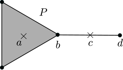
In this subsection we introduce mean dimension with potential for $\mathbb{R}^{d}$-actions. Let $P$ be a finite simplicial complex. (Here “finite” means that the number of faces is finite. In this paper we do not consider infinite simplicial complexes. Simplicial complexes are always finite.) For a point $a\in P$ we define $\dim_{a}P$ as the maximum of $\dim\Delta$ where $\Delta$ runs over all simplices of $P$ containing $a$. We call $\dim_{a}P$ the local dimension of $P$ at $a$. See Figure 1. (This is the same as [Tsu20, Fig. 1].)

Figure 1. Here $P$ has four vertexes (denoted by dots), four $1$-dimensional simplexes and one $2$-dimensional simplex. The points $b$ and $d$ are vertexes of $P$ wheres $a$ and $c$ are not. We have $\dim_{a}P=\dim_{b}P=2$ and $\dim_{c}P=\dim_{d}P=1$.

Let $(\mathcal{X},\mathbf{d})$ be a compact metric space. Let $\mathcal{Y}$ be a topological space and $f\colon\mathcal{X}\to\mathcal{Y}$ a continuous map. For a positive number $\varepsilon$ we call $f$ an $\varepsilon$-embedding if we have $\mathrm{Diam}f^{-1}(y)<\varepsilon$ for all $y\in\mathcal{Y}$. Let $\varphi:\mathcal{X}\to\mathbb{R}$ be a continuous function. We define the $\varepsilon$-width dimension with potential by

(1$$\cdot \begin{split}&\mathrm{Widim}_{\varepsilon}(\mathcal{X},\mathbf{d},\varphi)\\ &=\inf\left\{\max_{x\in\mathcal{X}}\left(\dim_{f(x)}P+\varphi(x)\right)\middle|\parbox{216.81pt}{\centering$P$ is a finite simplicial complex and $f:\mathcal{X}\to P$ is an $\varepsilon$-embedding\@add@centering}\right\}.\end{split}$$7)

Let $d$ be a natural number. We consider that $\mathbb{R}^{d}$ is equipped with the Euclidean topology and standard additive group structure. We denote the standard Lebesgue measure on $\mathbb{R}^{d}$ by $\mathbf{m}$. Let $T\colon\mathbb{R}^{d}\times\mathcal{X}\to\mathcal{X}$ be a continuous action of $\mathbb{R}^{d}$ on a compact metrizable space $\mathcal{X}$. Let $\mathbf{d}$ be a metric on $\mathcal{X}$ compatible with the topology, and let $\varphi\colon\mathcal{X}\to\mathbb{R}$ be a continuous function. For a bounded Borel subset $A\subset\mathbb{R}^{d}$ we define a new metric $\mathbf{d}_{A}$ and a new function $\varphi_{A}\colon\mathcal{X}\to\mathbb{R}$ by

$$\mathbf{d}_{A}(x,y)=\sup_{u\in A}\mathbf{d}(T^{u}x,T^{u}y),\quad\varphi_{A}(x)=\int_{A}\varphi(T^{u}x)\,d\mathbf{m}(u).$$

If $\varphi(x)\geq 0$ for all $x\in\mathcal{X}$ then we have:

1. Subadditivity: For bounded Borel subsets $A,B\subset\mathbb{R}^{d}$

   $$\mathrm{Widim}_{\varepsilon}\left(\mathcal{X},\mathbf{d}_{A\cup B},\varphi_{A\cup B}\right)\leq\mathrm{Widim}_{\varepsilon}\left(\mathcal{X},\mathbf{d}_{A},\varphi_{A}\right)+\mathrm{Widim}_{\varepsilon}\left(\mathcal{X},\mathbf{d}_{B},\varphi_{B}\right).$$

2. Monotonicity: If $A\subset B$ then

   $$0\leq\mathrm{Widim}_{\varepsilon}\left(\mathcal{X},\mathbf{d}_{A},\varphi_{A}\right)\leq\mathrm{Widim}_{\varepsilon}\left(\mathcal{X},\mathbf{d}_{B},\varphi_{B}\right).$$

3. Invariance: For $a\in\mathbb{R}^{d}$ and a bounded Borel subset $A\subset\mathbb{R}^{d}$

   $$\mathrm{Widim}_{\varepsilon}\left(\mathcal{X},\mathbf{d}_{a+A},\varphi_{a+A}\right)=\mathrm{Widim}_{\varepsilon}\left(\mathcal{X},\mathbf{d}_{A},\varphi_{A}\right),$$

   where $a+A=\{a+u\mid u\in A\}$.

Notice that we need to assume the nonnegativity of $\varphi$ for the properties (1) and (2).

For a positive number $L$ we denote $\mathbf{d}_{[0,L)^{d}}$ and $\varphi_{[0,L)^{d}}$ by $\mathbf{d}_{L}$ and $\varphi_{L}$ respectively for simplicity. We define the mean dimension with potential of $\left(\mathcal{X},T,\varphi\right)$ by

(1$$\cdot \mathrm{mdim}\left(\mathcal{X},T,\varphi\right)=\lim_{\varepsilon\to 0}\left(\lim_{L\to\infty}\frac{\mathrm{Widim}_{\varepsilon}(\mathcal{X},\mathbf{d}_{L},\varphi_{L})}{L^{d}}\right).$$8)

This is a topological invariant, namely its value is independent of the choice of the metric $\mathbf{d}$. Notice that we do not assume the nonnegativity of $\varphi$ in the definition (1$\cdot$8).

We need to check that the limits in the definition (1$\cdot$8) exist. The limit with respect to $\varepsilon$ exists because $\mathrm{Widim}_{\varepsilon}(\mathcal{X},\mathbf{d}_{L},\varphi_{L})$ is monotone in $\varepsilon$. We prove the existence of the limit with respect to $L$ in the next lemma.

Lemma 1.1.

The limit $\displaystyle\lim_{L\to\infty}\mathrm{Widim}_{\varepsilon}(\mathcal{X},\mathbf{d}_{L},\varphi_{L})/L^{d}$ exists in the definition (1$\cdot$8).

Proof.

Let $c$ be the minimum of $\varphi(x)$ over $x\in\mathcal{X}$ and set $\psi(x)=\varphi(x)-c$. Then $\psi$ is a nonnegative function with

$$\mathrm{Widim}_{\varepsilon}\left(\mathcal{X},\mathbf{d}_{A},\psi_{A}\right)=\mathrm{Widim}_{\varepsilon}\left(\mathcal{X},\mathbf{d}_{A},\varphi_{A}\right)-c\,\mathbf{m}(A).$$

Set $h(A)=\mathrm{Widim}_{\varepsilon}\left(\mathcal{X},\mathbf{d}_{A},\psi_{A}\right)$. It is enough to prove that the limit $\displaystyle\lim_{L\to\infty}h\left([0,L)^{d}\right)/L^{d}$ exists. For $0<L<R$, let $n=\lfloor R/L\rfloor$ be the integer part of $R/L$. We have

$$[0,R)^{d}\subset\bigcup_{u\in\mathbb{Z}^{d}\cap[0,n]^{d}}\left(Lu+[0,L)^{d}\right).$$

Since $\psi$ is nonnegative, $h(A)$ satisfies the subadditivity, monotonicity and invariance. Hence

$$h\left([0,R)^{d}\right)\leq(n+1)^{d}\cdot h\left([0,L)^{d}\right).$$

Dividing this by $R^{d}$ and letting $R\to\infty$, we get

$$\limsup_{R\to\infty}\frac{h\left([0,R)^{d}\right)}{R^{d}}\leq\frac{h\left([0,L)^{d}\right)}{L^{d}}.$$

Then letting $L\to\infty$ we get

$$\limsup_{R\to\infty}\frac{h\left([0,R)^{d}\right)}{R^{d}}\leq\liminf_{L\to\infty}\frac{h\left([0,L)^{d}\right)}{L^{d}}.$$

Therefore the limit $\displaystyle\lim_{L\to\infty}h\left([0,L)^{d}\right)/L^{d}$ exists. ∎

Remark 1.2.

By the Ornstein–Weiss quasi-tiling argument ([OS87], [Gro99, §1.3.1]) we can also prove that for any Følner sequence $A_{1},A_{2},A_{3},\dots$ of $\mathbb{R}^{d}$ the limit

$$\lim_{n\to\infty}\frac{\mathrm{Widim}_{\varepsilon}(\mathcal{X},\mathbf{d}_{A_{n}},\varphi_{A_{n}})}{\mathbf{m}(A_{n})}$$

exists and that its value is independent of the choice of a Følner sequence. In particular, we can define the mean dimension with potential by

$$\mathrm{mdim}\left(\mathcal{X},T,\varphi\right)=\lim_{\varepsilon\to 0}\left(\lim_{R\to\infty}\frac{\mathrm{Widim}_{\varepsilon}(\mathcal{X},\mathbf{d}_{B_{R}},\varphi_{B_{R}})}{\mathbf{m}(B_{R})}\right),$$

where $B_{R}=\{u\in\mathbb{R}^{d}\mid|u|\leq R\}$.

1.3. Main result

Let $\mathcal{X}$ be a compact metrizable space. Recall that we have denoted by $\mathscr{D}(\mathcal{X})$ the set of metrics $\mathbf{d}$ on $\mathcal{X}$ compatible with the given topology. Let $T\colon\mathbb{R}^{d}\times\mathcal{X}\to\mathcal{X}$ be a continuous action. A Borel probability measure $\mu$ on $\mathcal{X}$ is said to be $T$-invariant if $\mu(T^{-u}A)=\mu(A)$ for all $u\in\mathbb{R}^{d}$ and all Borel subsets $A\subset\mathcal{X}$. We define $\mathscr{M}^{T}(\mathcal{X})$ as the set of all $T$-invariant Borel probability measures $\mu$ on $\mathcal{X}$.

Take a metric $\mathbf{d}\in\mathscr{D}(\mathcal{X})$ and a measure $\mu\in\mathscr{M}^{T}(\mathcal{X})$. We randomly choose a point $x\in\mathcal{X}$ according to the distribution $\mu$ and consider the orbit $\{T^{u}x\}_{u\in\mathbb{R}^{d}}$. For a positive number $\varepsilon$ we define the rate distortion function $R(\mathbf{d},\mu,\varepsilon)$ as the minimum bits per unit volume for describing $\{T^{u}x\}_{u\in\mathbb{R}^{d}}$ with average distortion bounded by $\varepsilon$ with respect to $\mathbf{d}$. The precise definition of $R(\mathbf{d},\mu,\varepsilon)$ is given in §2.3.

We define the upper and lower rate distortion dimensions by

$$\overline{\mathrm{rdim}}(\mathcal{X},T,\mathbf{d},\mu)=\limsup_{\varepsilon\to 0}\frac{R(\mathbf{d},\mu,\varepsilon)}{\log(1/\varepsilon)},\quad\underline{\mathrm{rdim}}(\mathcal{X},T,\mathbf{d},\mu)=\liminf_{\varepsilon\to 0}\frac{R(\mathbf{d},\mu,\varepsilon)}{\log(1/\varepsilon)}.$$

The following is the main result of this paper.

Theorem 1.3 (Main theorem).

Let $T\colon\mathbb{R}^{d}\times\mathcal{X}\to\mathcal{X}$ be a continuous action of $\mathbb{R}^{d}$ on a compact metrizable space $\mathcal{X}$. Let $\varphi\colon\mathcal{X}\to\mathbb{R}$ be a continuous function. Then for any metric $\mathbf{d}\in\mathscr{D}(\mathcal{X})$

$$\mathrm{mdim}\left(\mathcal{X},T,\varphi\right)\leq\sup_{\mu\in\mathscr{M}^{T}(\mathcal{X})}\left(\underline{\mathrm{rdim}}(\mathcal{X},T,\mathbf{d},\mu)+\int_{\mathcal{X}}\varphi\,d\mu\right).$$

We propose a conjecture:

Conjecture 1.4.

In the setting of Theorem 1.3 we have

$$\begin{split}\mathrm{mdim}(\mathcal{X},T,\varphi)&=\min_{\mathbf{d}\in\mathscr{D}(\mathcal{X})}\left\{\sup_{\mu\in\mathscr{M}^{T}(\mathcal{X})}\left(\underline{\mathrm{rdim}}(\mathcal{X},T,\mathbf{d},\mu)+\int_{\mathcal{X}}\varphi\,d\mu\right)\right\}\\ &=\min_{\mathbf{d}\in\mathscr{D}(\mathcal{X})}\left\{\sup_{\mu\in\mathscr{M}^{T}(\mathcal{X})}\left(\overline{\mathrm{rdim}}(\mathcal{X},T,\mathbf{d},\mu)+\int_{\mathcal{X}}\varphi\,d\mu\right)\right\}.\end{split}$$

We think that probably we can prove this conjecture if $T\colon\mathbb{R}^{d}\times\mathcal{X}\to\mathcal{X}$ is a free minimal action. The proof will be rather lengthy and technically heavy. We postpone it to Part II of this series of papers.

Along the way to prove Theorem 1.3, we will introduce mean Hausdorff dimension with potential and metric mean dimension with potential for $\mathbb{R}^{d}$-actions and establish their basic properties. In particular we prove:

1. Mean Hausdorff dimension with potential bounds $\mathrm{mdim}\left(\mathcal{X},T,\varphi\right)$ from above (Theorem 3.4).

2. We can construct invariant probability measures which capture the complexity of dynamics expressed by mean Hausdorff dimension with potential (Dynamical Frostman’s lemma; Theorem 3.7).

3. Metric mean dimension with potential bounds $\displaystyle\overline{\mathrm{rdim}}(\mathcal{X},T,\mathbf{d},\mu)+\int_{\mathcal{X}}\varphi\,d\mu$ from above (Proposition 3.5).

4. Metric mean dimension with potential can be calculated by using only “local” information (Theorem 7.1).

The results (1) and (2) will be used in the proof of Theorem 1.3. The results (3) and (4) are not used in the proof of Theorem 1.3. We plan to use (3) in Part II of this series of papers. The result (4) may be useful when we study geometric examples of [Gro99, MT15, Tsu18] in a future.

1.4. Organization of the paper

In §2 we prepare basic definitions and results on mutual information and rate distortion theory. In §3 we introduce mean Hausdorff dimension with potential and metric mean dimension with potential for $\mathbb{R}^{d}$-actions. We also state their fundamental properties in §3. The proofs will be given in §5 and §6. Theorem 1.3 (Main Theorem) follows from the properties of mean Hausdorff dimension with potential stated in §3. In §4 we prepare some basic results on mean dimension theory of $\mathbb{Z}^{d}$-actions. They will be used in §5. In §5 we prove that $\mathrm{mdim}(\mathcal{X},T,\varphi)$ is bounded from above by mean Hausdorff dimension with potential. In §6 we prove dynamical Frostman’s lemma. In §7 we prove that metric mean dimension with potential can be calculated by using certain local information. §7 is independent of the proof of Theorem 1.3.

2. Mutual information and rate distortion theory

We prepare basics of rate distortion theory in this section. Throughout this paper $\log x$ denotes the logarithm of base two. The natural logarithm is denoted by $\ln x$:

$$\log x=\log_{2}x,\quad\ln x=\log_{e}x.$$

This section is rather long. This is partly because we have to be careful of measure theoretic details. Hopefully this section will become a useful reference in a future study of mean dimension of $\mathbb{R}^{d}$-actions. At the first reading, readers may skip the whole of Subsection 2.1 and most of Subsection 2.2. The crucial parts of this section are only the definition of mutual information in §2.2 and the definition of rate distortion function in §2.3. All the rest of this section are technical details.

2.1. Measure theoretic preparations

We need to prepare some basic results on measure theory. A measurable space is a pair $(\mathcal{X},\mathcal{A})$ of a set $\mathcal{X}$ and its $\sigma$-algebra $\mathcal{A}$. Two measurable spaces $(\mathcal{X},\mathcal{A})$ and $(\mathcal{Y},\mathcal{B})$ are said to be isomorphic if there exists a bijection $f\colon\mathcal{X}\to\mathcal{Y}$ such that both $f$ and $f^{-1}$ are measurable (i.e. $f(\mathcal{A})=\mathcal{B}$).

For a topological space $\mathcal{X}$, its Borel $\sigma$-algebra $\mathcal{B}_{\mathcal{X}}$ is the minimum $\sigma$-algebra containing all open subsets of $\mathcal{X}$. A Polish space is a topological space $\mathcal{X}$ admitting a metric $\mathbf{d}$ for which $(\mathcal{X},\mathbf{d})$ is a complete separable metric space.

A measurable space $(\mathcal{X},\mathcal{A})$ is said to be a standard Borel space if there exists a Polish space $\mathcal{Y}$ for which $(\mathcal{X},\mathcal{A})$ is isomorphic to $(\mathcal{Y},\mathcal{B}_{\mathcal{Y}})$ as measurable spaces. It is known that any two uncountable standard Borel spaces are isomorphic to each other (the Borel isomorphism theorem [Sri98, Theorem 3.3.13]). Therefore every standard Borel space is isomorphic to one of the following measurable spaces:

• A finite set $A$ with its discrete $\sigma$-algebra $2^{A}:=\{\text{subset of $A$}\}$.

• The set of natural numbers $\mathbb{N}$ with its discrete $\sigma$-algebra $2^{\mathbb{N}}:=\{\text{subset of $\mathbb{N}$}\}$.

• The Cantor set $\mathcal{C}=\{0,1\}^{\mathbb{N}}$ with its Borel $\sigma$-algebra $\mathcal{B}_{\mathcal{C}}$. (Here $\{0,1\}$ is endowed with the discrete topology and the topology of $\mathcal{C}$ is the product topology.)

An importance of standard Borel spaces is that we can prove the existence of regular conditional distribution under the assumption of “standard Borel”. Let $(\mathcal{X},\mathcal{A})$ and $(\mathcal{Y},\mathcal{B})$ be measurable spaces. A transition probability on $\mathcal{X}\times\mathcal{Y}$ is a map $\nu:\mathcal{X}\times\mathcal{B}\to[0,1]$ such that

• for every $x\in\mathcal{X}$, the map $\mathcal{B}\ni B\mapsto\nu(x,B)\in[0,1]$ is a probability measure on $(\mathcal{Y},\mathcal{B})$,

• for every $B\in\mathcal{B}$, the map $\mathcal{X}\ni x\mapsto\nu(x,B)\in[0,1]$ is measurable.

We often denote $\nu(x,B)$ by $\nu(B|x)$.

For two measurable spaces $(\mathcal{X},\mathcal{A})$ and $(\mathcal{Y},\mathcal{B})$ we denote their product by $(\mathcal{X}\times\mathcal{Y},\mathcal{A}\otimes\mathcal{B})$ where $\mathcal{A}\otimes\mathcal{B}$ is the minimum $\sigma$-algebra containing all the rectangles $A\times B$ $(A\in\mathcal{A},B\in\mathcal{B})$. For any $E\in\mathcal{A}\otimes\mathcal{B}$, it is known that the section $E_{x}:=\{y\in\mathcal{Y}\mid(x,y)\in E\}$ belongs to $\mathcal{B}$ for every $x\in\mathcal{X}$. (This fact is a part of the Fubini theorem. It can be easily proved by using Dynkin’s $\pi$-$\lambda$ theorem [Dur10, p.402 Theorem A.1.4].) Moreover, if $(\mathcal{Y},\mathcal{B})$ is a standard Borel space, then for any transition probability $\nu$ on $\mathcal{X}\times\mathcal{Y}$ and any $E\in\mathcal{A}\otimes\mathcal{B}$ the map $\mathcal{X}\ni x\mapsto\nu(E_{x}|x)\in[0,1]$ is measurable [Sri98, Proposition 3.4.24].

A probability space is a triplet $(\Omega,\mathcal{F},\mathbb{P})$ where $(\Omega,\mathcal{F})$ is a measurable space and $\mathbb{P}$ is a probability measure defined on it. Let $X\colon\Omega\to\mathcal{X}$ be a measurable map from a probability space $(\Omega,\mathcal{F},\mathbb{P})$ to a Borel space $(\mathcal{X},\mathcal{A})$. We denote the push-forward measure $X_{*}\mathbb{P}$ by $\mathrm{Law}X$ and call it the law of $X$ or the distribution of $X$. (Here $X_{*}\mathbb{P}(A)=\mathbb{P}\left(X\in A\right)=\mathbb{P}\left(X^{-1}(A)\right)$ for $A\in\mathcal{A}$.)

The next theorem is a fundamental result. It guarantees the existence of regular conditional probability. For the proof, see [IW81, p.15 Theorem 3.3 and its Corollary] or Gray [Gra09, p. 182 Corollary 6.2].

Theorem 2.1 (Existence of regular conditional distribution).

Let $(\Omega,\mathcal{F},\mathbb{P})$ be a probability space, and $(\mathcal{X},\mathcal{A})$ and $(\mathcal{Y},\mathcal{B})$ standard Borel spaces. Let $X:\Omega\to\mathcal{X}$ and $Y:\Omega\to\mathcal{Y}$ be measurable maps, and set $\mu:=\mathrm{Law}X$. Then there exists a transition probability $\nu$ on $\mathcal{X}\times\mathcal{Y}$ such that for any $E\in\mathcal{A}\otimes\mathcal{B}$ we have

$$\mathbb{P}\left((X,Y)\in E\right)=\int_{\mathcal{X}}\nu(E_{x}|x)\,d\mu(x).$$

If a transition probability $\nu^{\prime}$ on $\mathcal{X}\times\mathcal{Y}$ satisfies the same property then there exists a $\mu$-null set $N\in\mathcal{A}$ such that $\nu(B|x)=\nu^{\prime}(B|x)$ for all $x\in\mathcal{X}\setminus N$ and $B\in\mathcal{B}$.

The transition probability $\nu(\cdot|x)$ in this theorem is called the regular conditional distribution of $Y$ given $X=x$. We sometimes denote $\nu(B|x)$ by $\mathbb{P}(Y\in B|X=x)$ for $x\in\mathcal{X}$ and $B\in\mathcal{B}$. If $\mathcal{X}$ and $\mathcal{Y}$ are finite sets, then this coincides with the elementary notion of conditional probability:

$$\mathbb{P}(Y\in B|X=x)=\frac{\mathbb{P}(X=x,Y\in B)}{\mathbb{P}(X=x)},\quad\left(\text{if }\mathbb{P}(X=x)\neq 0\right).$$

In this case we usually denote $\nu\left(\{y\}|x\right)$ by $\nu(y|x)$ $(x\in\mathcal{X},y\in\mathcal{Y})$ and call it a conditional probability mass function.

By using the notion of regular conditional distribution, we can introduce the definition of conditional independence of random variables. Let $(\Omega,\mathbb{P})$ be a probability space and $(\mathcal{X},\mathcal{A}),(\mathcal{Y},\mathcal{B}),(\mathcal{Z},\mathcal{C})$ standard Borel spaces. Let $X\colon\Omega\to\mathcal{X}$, $Y\colon\Omega\to\mathcal{Y}$ and $Z\colon\Omega\to\mathcal{Z}$ be measurable maps. We say that $X$ and $Y$ are conditionally independent given $Z$ if we have

(2$$\cdot \mathbb{P}\left((X,Y)\in A\times B|Z=z\right)=\mathbb{P}\left(X\in A|Z=z\right)\cdot\mathbb{P}\left(Y\in B|Z=z\right)$$1)

for $Z_{*}\mathbb{P}$-a.e. $z\in\mathcal{Z}$ and all $A\in\mathcal{A}$ and $B\in\mathcal{B}$. Here $Z_{*}\mathbb{P}$ is the push-forward measure of $\mathbb{P}$ by $Z$. The left-hand side of (2$\cdot$1) is the conditional regular distribution of $(X,Y)\colon\Omega\to\mathcal{X}\times\mathcal{Y}$ given $Z=z$. The right-hand side is the multiple of the conditional distribution of $X$ given $Z=z$ and the conditional distribution of $Y$ given $Z=z$.

At the end of this subsection we explain the log-sum inequality. This will be used in the next subsection.

Lemma 2.2 (Log-sum inequality).

Let $(\mathcal{X},\mathcal{A})$ be a measurable space. Let $\mu$ be a measure on it with $0<\mu(\mathcal{X})<\infty$. Let $f$ and $g$ be nonnegative measurable functions defined on $\mathcal{X}$. Suppose that $g$ is $\mu$-integrable and $g(x)>0$ for $\mu$-a.e. $x\in\mathcal{X}$. Then

$$\left(\int_{\mathcal{X}}f(x)\,d\mu(x)\right)\log\frac{\int_{\mathcal{X}}f(x)\,d\mu(x)}{\int_{\mathcal{X}}g(x)\,d\mu(x)}\leq\int_{\mathcal{X}}f(x)\log\frac{f(x)}{g(x)}\,d\mu(x).$$

In particular, if the left-hand side is infinite then the right-hand side is also infinite.

Here we assume $0\log\frac{0}{a}=0$ for all $a>0$.

Proof.

Set $\phi(t)=t\log t$ for $t\geq 0$. Since $\phi^{\prime\prime}(t)=\log e/t>0$ for $t>0$, this is a convex function. We define a probability measure $w$ on $\mathcal{X}$ by

$$w(A)=\frac{\int_{A}g\,d\mu}{\int_{\mathcal{X}}g\,d\mu}\quad(A\subset\mathcal{X}).$$

The Radon–Nikodim derivative of $w$ by $\mu$ is given by

$$\frac{dw}{d\mu}=\frac{g}{\int_{\mathcal{X}}g\,d\mu}.$$

By Jensen’s inequality

(2$$\cdot \phi\left(\int_{\mathcal{X}}\frac{f}{g}\,dw\right)\leq\int_{\mathcal{X}}\phi\left(\frac{f}{g}\right)\,dw.$$2)

Here, if the left-hand side is infinite, then the right-hand side is also infinite. We have

$$\phi\left(\int_{\mathcal{X}}\frac{f}{g}\,dw\right)=\phi\left(\frac{\int_{\mathcal{X}}f\,d\mu}{\int_{\mathcal{X}}g\,d\mu}\right)=\frac{\int_{\mathcal{X}}f\,d\mu}{\int_{\mathcal{X}}g\,d\mu}\log\frac{\int_{\mathcal{X}}f\,d\mu}{\int_{\mathcal{X}}g\,d\mu}.$$

The right-hand side of (2$\cdot$2) is

$$\int_{\mathcal{X}}\phi\left(\frac{f}{g}\right)\,dw=\frac{1}{\int_{\mathcal{X}}g\,d\mu}\int_{\mathcal{X}}g\phi\left(\frac{f}{g}\right)\,d\mu=\frac{1}{\int_{\mathcal{X}}g\,d\mu}\int_{\mathcal{X}}f\log\frac{f}{g}\,d\mu.$$

Therefore (2$\cdot$2) provides

$$\left(\int_{\mathcal{X}}f\,d\mu\right)\log\frac{\int_{\mathcal{X}}f\,d\mu}{\int_{\mathcal{X}}g\,d\mu}\leq\int_{\mathcal{X}}f\log\frac{f}{g}\,d\mu.$$

∎

The following is the finitary version of the log-sum inequality:

Corollary 2.3.

Let $a_{1},\dots,a_{n}$ be nonnegative numbers and $b_{1},\dots,b_{n}$ positive numbers. Then

$$\left(\sum_{i=1}^{n}a_{i}\right)\log\frac{\sum_{i=1}^{n}a_{i}}{\sum_{i=1}^{n}b_{i}}\leq\sum_{i=1}^{n}a_{i}\log\frac{a_{i}}{b_{i}}.$$

Proof.

Apply Lemma 2.2 to the finite set $\mathcal{X}=\{1,2,\dots,n\}$ with the discrete $\sigma$-algebra and the counting measure. ∎

2.2. Mutual information

Let $(\Omega,\mathcal{F},\mathbb{P})$ be a probability space. We assume that all random variables in this subsection are defined on $(\Omega,\mathcal{F},\mathbb{P})$. In this paper a finite set is always assumed to be endowed with the discrete topology and the discrete $\sigma$-algebra (i.e. the set of all subsets). The purpose of this subsection is to define and study mutual information. A basic reference of mutual information is the book of Cover–Thomas [CT06]. A mathematically sophisticated presentation is given in the book of Gray [Gra11].

First we define the Shannon entropy. Let $(\mathcal{X},\mathcal{A})$ be a finite set with the discrete $\sigma$-algebra, and let $X\colon\Omega\to\mathcal{X}$ be a measurable map. We define the Shannon entropy of $X$ by

$$H(X)=-\sum_{x\in\mathcal{X}}\mathbb{P}(X=x)\log\mathbb{P}(X=x).$$

Here we assume $0\log 0=0$ as usual.

Next we define the mutual information. Let $(\mathcal{X},\mathcal{A})$ and $(\mathcal{Y},\mathcal{B})$ be two measurable spaces and let $X\colon\Omega\to\mathcal{X}$ and $Y\colon\Omega\to\mathcal{Y}$ be measurable maps. We want to define the mutual information $I(X;Y)$. Intuitively $I(X;Y)$ measure the amount of information shared by the random variables $X$ and $Y$.

• Case I: Suppose $(\mathcal{X},\mathcal{A})$ and $(\mathcal{Y},\mathcal{B})$ are finite sets with the discrete $\sigma$-algebras. Then we define

  (2$$\cdot I(X;Y)=H(X)+H(Y)-H(X,Y),$$3)

  where $H(X,Y)$ is the Shannon entropy of the measurable map $(X,Y):\Omega\to\mathcal{X}\times\mathcal{Y}$. Since $H(X,Y)\leq H(X)+H(Y)$, the mutual information $I(X;Y)$ is always nonnegative. The explicit formula is given by

  $$I(X;Y)=\sum_{x\in\mathcal{X},y\in\mathcal{Y}}\mathbb{P}(X=x,Y=y)\log\frac{\mathbb{P}(X=x,Y=y)}{\mathbb{P}(X=x)\mathbb{P}(Y=y)}.$$

  Here we assume $0\log\frac{0}{a}=0$ for any $a\geq 0$. The mutual information $I(X;Y)$ satisfies the following natural monotonicity: Let $\mathcal{X}^{\prime}$ and $\mathcal{Y}^{\prime}$ be finite sets (endowed with the discrete $\sigma$-algebras), and let $f\colon\mathcal{X}\to\mathcal{X}^{\prime}$ and $g\colon\mathcal{Y}\to\mathcal{Y}^{\prime}$ be any maps. Then it follows from the log-sum inequality (Corollary 2.3) that

  (2$$\cdot I\left(f(X);g(Y)\right)\leq I(X;Y).$$4)

• Case II: Here we define $I(X;Y)$ for general random variables $X$ and $Y$. (Namely $\mathcal{X}$ and $\mathcal{Y}$ may be infinite sets.) Let $\mathcal{X}^{\prime}$ and $\mathcal{Y}^{\prime}$ be arbitrary finite sets, and let $f\colon\mathcal{X}\to\mathcal{X}^{\prime}$ and $g\colon\mathcal{Y}\to\mathcal{Y}^{\prime}$ be any measurable maps. Then we can consider $I\left(f(X);g(Y)\right)$ by Case I. We define $I(X;Y)$ as the supremum of $I\left(f(X);g(Y)\right)$ over all finite sets $\mathcal{X}^{\prime},\mathcal{Y}^{\prime}$ and measurable maps $f\colon\mathcal{X}\to\mathcal{X}^{\prime}$ and $g\colon\mathcal{Y}\to\mathcal{Y}^{\prime}$. The mutual information $I(X,Y)$ is always nonnegative and symmetric: $I(X;Y)=I(Y;X)\geq 0$.

  If $f\colon\mathcal{X}\to\mathcal{X}^{\prime}$ and $g\colon\mathcal{Y}\to\mathcal{Y}^{\prime}$ are measurable maps to some other measurable spaces $(\mathcal{X}^{\prime},\mathcal{A}^{\prime})$ and $(\mathcal{Y}^{\prime},\mathcal{B}^{\prime})$ (not necessarily finite sets) then we have $I\left(f(X);g(Y)\right)\leq I\left(X;Y\right)$.

  If $\mathcal{X}$ and $\mathcal{Y}$ are finite sets, then the definition of Case II is compatible with Case I by the monotonicity (2$\cdot$4).

If $(\mathcal{X},\mathcal{A})$ and $(\mathcal{Y},\mathcal{B})$ are standard Borel spaces, then we can consider the regular conditional distribution of $Y$ given $X=x$. We denote

$$\nu(B|x)=\mathbb{P}(Y\in B|X=x)\quad(x\in\mathcal{X},B\in\mathcal{B}).$$

Let $\mu=X_{*}\mathbb{P}$ be the push-forward measure of $\mathbb{P}$ by $X$. The distribution of $(X,Y)$ is determined by $\mu$ and $\nu$. Hence the mutual information $I(X;Y)$ is also determined by $\mu$ and $\nu$. Therefore we sometimes denote $I(X;Y)$ by $I(\mu,\nu)$. An importance of this description comes from the fact that $I(\mu,\nu)$ is a concave function in $\mu$ and a convex function in $\nu$ (Proposition 2.10 below).

In the rest of this subsection we prepare several basic properties of mutual information. They are rather heavy. Readers may skip to the next subsection at the first reading.

If $(\mathcal{X},\mathcal{A})$ is a standard Borel space and if $\mathcal{Y}$ is a finite set, then we can express $I(X;Y)$ in another convenient way. For $x\in\mathcal{X}$ we set

$$H(Y|X=x)=-\sum_{y\in\mathcal{Y}}\mathbb{P}\left(Y=y|X=x\right)\log\mathbb{P}\left(Y=y|X=x\right).$$

We define the conditional entropy of $Y$ given $X$ by

$$H(Y|X)=\int_{\mathcal{X}}H(Y|X=x)\,d\mu(x),\quad(\mu:=X_{*}\mathbb{P}).$$

The next theorem is given in the book of Gray [Gra11, p. 213, Lemma 7.20].

Theorem 2.4.

Let $X$ and $Y$ be random variables taking values in a standard Borel space $(\mathcal{X},\mathcal{A})$ and a finite set $\mathcal{Y}$ respectively. Then we have

$$I(X;Y)=H(Y)-H(Y|X).$$

When both $\mathcal{X}$ and $\mathcal{Y}$ are finite sets, this theorem is a very well-known result. A point of the theorem is that we do not need to assume that $\mathcal{X}$ is a finite set.

The following is also a basic result. This is given in [Gra11, p. 211, Lemma 7.18].

Theorem 2.5.

Let $(\mathcal{X},\mathcal{A})$ and $\left(\mathcal{Y},\mathcal{B}\right)$ be standard Borel spaces. Then there exist sequences of measurable maps $f_{n}\colon\mathcal{X}\to\mathcal{X}_{n}$ and $g_{n}\colon\mathcal{Y}\to\mathcal{Y}_{n}$ to some finite sets $\mathcal{X}_{n}$ and $\mathcal{Y}_{n}$ $(n\geq 1)$ for which the following statement holds: If $X$ and $Y$ are random variables taking values in $(\mathcal{X},\mathcal{A})$ and $\left(\mathcal{Y},\mathcal{B}\right)$ respectively, then

$$I(X;Y)=\lim_{n\to\infty}I\left(f_{n}(X);g_{n}(Y)\right).$$

Sketch of the proof.

Standard Borel spaces are isomorphic to either countable sets or the Cantor sets. The case of countable sets is easier. So we assume that both $\mathcal{X}$ and $\mathcal{Y}$ are the Cantor set $\{0,1\}^{\mathbb{N}}$. Let $f_{n}\colon\mathcal{X}\to\{0,1\}^{n}$ and $g_{n}\colon\mathcal{Y}\to\{0,1\}^{n}$ be the natural projections to the first $n$ coordinates. Then we can check that $f_{n}$ and $g_{n}$ satisfy the statement. ∎

Lemma 2.6.

Let $X_{n}$ and $Y_{n}$ $(n\geq 1)$ be sequences of random variables taking values in finite sets $\mathcal{X}$ and $\mathcal{Y}$ respectively. Suppose $(X_{n},Y_{n})$ converges to $(X,Y)$ in law. (Namely $\mathbb{P}\left(X_{n}=x,Y_{n}=y\right)\to\mathbb{P}(X=x,Y=y)$ as $n\to\infty$ for all $(x,y)\in\mathcal{X}\times\mathcal{Y}$.) Then $I(X_{n};Y_{n})$ converges to $I(X;Y)$ as $n\to\infty$.

Proof.

This immediately follows from the definition (2$\cdot$3) in Case I above. ∎

Lemma 2.7 (Subadditivity of mutual information).

Let $X,Y,Z$ be random variables taking values in standard Borel spaces $(\mathcal{X},\mathcal{A}),(\mathcal{Y},\mathcal{B}),(\mathcal{Z},\mathcal{C})$ respectively. Suppose that $X$ and $Y$ are conditionally independent given $Z$. Then

$$I\left(X,Y;Z\right)\leq I(X;Z)+I(Y;Z),$$

where $I\left(X,Y;Z\right)=I\left((X,Y);Z\right)$ is the mutual information between the random variables $(X,Y)$ and $Z$.

Proof.

Let $f\colon\mathcal{X}\to\mathcal{X}^{\prime}$ and $g\colon\mathcal{Y}\to\mathcal{Y}^{\prime}$ be measurable maps to some finite sets $\mathcal{X}^{\prime}$ and $\mathcal{Y}^{\prime}$. Then by Theorem 2.4

$$I\left(f(X),g(Y);Z\right)=H\left(f(X),g(Y)\right)-H\left(f(X),g(Y)|Z\right).$$

We have [CT06, Theorem 2.6.6]

$$H\left(f(X),g(Y)\right)\leq H\left(f(X)\right)+H\left(g(Y)\right).$$

The random variables $f(X)$ and $g(Y)$ are conditionally independent given $Z$. Hence

$$H\left(f(X),g(Y)|Z\right)=H\left(f(X)|Z\right)+H\left(g(Y)|Z\right).$$

Therefore

$$\begin{split}I\left(f(X),g(Y);Z\right)&\leq\left\{H\left(f(X)\right)-H\left(f(X)|Z\right)\right\}+\left\{H\left(g(Y)\right)-H\left(g(Y)|Z\right)\right\}\\ &=I\left(f(X);Z\right)+I\left(g(Y);Z\right).\end{split}$$

We have $I\left(X,Y;Z\right)=\sup_{f,g}I\left(f(X),g(Y);Z\right)$ where $f\colon\mathcal{X}\to\mathcal{X}^{\prime}$ and $g\colon\mathcal{Y}\to\mathcal{Y}^{\prime}$ run over all measurable maps to some finite sets. This follows from the fact that $\mathcal{A}\otimes\mathcal{B}$ is generated by rectangles $A\times B$ $(A\in\mathcal{A},B\in\mathcal{B})$ [Gra11, p.175 Lemma 7.3]. Therefore we get

$$I\left(X,Y;Z\right)\leq I(X;Z)+I(Y;Z).$$

∎

As we briefly mentioned above, the mutual information $I(\mu,\nu)$ is a concave function in a probability measure $\mu$ and a convex function in a transition probability $\nu$. Next we are going to establish this fact. We need some preparations.

For a finite set $\mathcal{Y}$, a probability mass function $p$ on $\mathcal{Y}$ is a nonnegative function on $\mathcal{Y}$ satisfying $\sum_{y\in\mathcal{Y}}p(y)=1$. For a probability mass function $p$ on $\mathcal{Y}$ we define

$$H(p)=-\sum_{y\in\mathcal{Y}}p(y)\log p(y).$$

Lemma 2.8 (Concavity of the Shannon entropy).

Let $\mathcal{Y}$ be a finite set and let $(\mathcal{Z},\mathcal{C},m)$ be a probability space. Suppose that we are given a probability mass function $p_{z}$ on $\mathcal{Y}$ for each $z\in\mathcal{Z}$ and that the map $\mathcal{Z}\ni z\mapsto p_{z}(y)\in[0,1]$ is measurable for each $y\in\mathcal{Y}$. We define a probability mass function $p$ on $\mathcal{Y}$ by

$$p(y)=\int_{\mathcal{Z}}p_{z}(y)\,dm(z).$$

Then

$$H(p)\geq\int_{\mathcal{Z}}H(p_{z})\,dm(z).$$

Proof.

From the log-sum inequality (Lemma 2.2),

$$-p(y)\log p(y)\geq-\int_{\mathcal{Z}}p_{z}(y)\log p_{z}(y)\,dm(z).$$

Summing this over $y\in\mathcal{Y}$, we get the statement. ∎

Lemma 2.9.

Let $\mathcal{X}$ and $\mathcal{Y}$ be finite sets and $(\mathcal{Z},\mathcal{C},m)$ a probability space. Let $\mu$ be a probability mass function on $\mathcal{X}$. Suppose that, for each $z\in\mathcal{Z}$, we are given a conditional probability mass function $\nu_{z}(y|x)$ in $x\in\mathcal{X}$ and $y\in\mathcal{Y}$ such that the map $\mathcal{Z}\ni z\mapsto\nu_{z}(y|x)\in[0,1]$ is measurable for each $(x,y)\in\mathcal{X}\times\mathcal{Y}$. We define

$$\nu(y|x)=\int_{\mathcal{Z}}\nu_{z}(y|x)\,dm(z),\quad(x\in\mathcal{X},y\in\mathcal{Y}).$$

Then

$$I(\mu,\nu)\leq\int_{\mathcal{Z}}I(\mu,\nu_{z})\,dm(z).$$

Proof.

For $y\in\mathcal{Y}$ we set

$$p_{z}(y)=\sum_{x\in\mathcal{X}}\mu(x)\nu_{z}(y|x),\quad p(y)=\sum_{x\in\mathcal{X}}\mu(x)\nu(y|x).$$

We have

$$I(\mu,\nu)=\sum_{x,y}\mu(x)\nu(y|x)\log\frac{\mu(x)\nu(y|x)}{\mu(x)p(y)},\quad I(\mu,\nu_{z})=\sum_{x,y}\mu(x)\nu_{z}(y|x)\log\frac{\mu(x)\nu_{z}(y|x)}{\mu(x)p_{z}(y)}.$$

Here we assume $0\log\frac{a}{0}=0$ for all $a\geq 0$.

We estimate each summand of $I(\mu,\nu)$ and $I(\mu,\nu_{z})$. We fix $(x,y)\in\mathcal{X}\times\mathcal{Y}$ with $\mu(x)p(y)>0$. We define a subset $\mathcal{Z}^{\prime}\subset\mathcal{Z}$ by

$$\mathcal{Z}^{\prime}=\{z\mid p_{z}(y)>0\}\supset\{z\mid\nu_{z}(y|x)>0\}.$$

Since $\mu(x)p(y)>0$, we have $m\left(\mathcal{Z}^{\prime}\right)>0$. We have

$$\mu(x)\nu(y|x)=\int_{\mathcal{Z}^{\prime}}\mu(x)\nu_{z}(y|x)\,dm(z),\quad\mu(x)p(y)=\int_{\mathcal{Z}^{\prime}}\mu(x)p_{z}(y)\,dm(z).$$

By the log-sum inequality (Lemma 2.2)

$$\begin{split}\mu(x)\nu(y|x)\log\frac{\mu(x)\nu(y|x)}{\mu(x)p(y)}&\leq\int_{\mathcal{Z}^{\prime}}\mu(x)\nu_{z}(y|x)\log\frac{\mu(x)\nu_{z}(y|x)}{\mu(x)p_{z}(y)}dm(z)\\ &=\int_{\mathcal{Z}}\mu(x)\nu_{z}(y|x)\log\frac{\mu(x)\nu_{z}(y|x)}{\mu(x)p_{z}(y)}dm(z).\end{split}$$

Taking sums over $(x,y)\in\mathcal{X}\times\mathcal{Y}$, we get the statement. ∎

Proposition 2.10 ($I(\mu,\nu)$ is concaive in $\mu$ and convex in $\nu$).

Let $(\mathcal{X},\mathcal{A})$ and $(\mathcal{Y},\mathcal{B})$ be standard Borel spaces, and let $(\mathcal{Z},\mathcal{C},m)$ be a probability space.

1. Let $\nu$ be a transition probability on $\mathcal{X}\times\mathcal{Y}$. Suppose that we are given a probability measure $\mu_{z}$ on $\mathcal{X}$ for each $z\in\mathcal{Z}$ such that the map $\mathcal{Z}\ni z\mapsto\mu_{z}(A)\in[0,1]$ is measurable for every $A\in\mathcal{A}$. We define a probability measure $\mu$ on $(\mathcal{X},\mathcal{A})$ by

   $$\mu(A)=\int_{\mathcal{Z}}\mu_{z}(A)\,dm(z),\quad(A\in\mathcal{A}).$$

   Then we have

   (2$$\cdot I(\mu,\nu)\geq\int_{\mathcal{Z}}I(\mu_{z},\nu)\,dm(z).$$5)

2. Let $\mu$ be a probability measure on $\mathcal{X}$. Suppose that we are given a transition probability $\nu_{z}$ on $\mathcal{X}\times\mathcal{Y}$ for each $z\in\mathcal{Z}$ such that the map $\mathcal{X}\times\mathcal{Z}\ni(x,z)\mapsto\nu_{z}(B|x)\in[0,1]$ is measurable with respect to $\mathcal{A}\otimes\mathcal{C}$ for each $B\in\mathcal{B}$. We define a transition probability $\nu$ on $\mathcal{X}\times\mathcal{Y}$ by

   $$\nu(B|x)=\int_{\mathcal{Z}}\nu_{z}(B|x)dm(z),\quad(x\in\mathcal{X},B\in\mathcal{B}).$$

   Then we have

   $$I(\mu,\nu)\leq\int_{\mathcal{Z}}I(\mu,\nu_{z})\,dm(z).$$

Proof.

(1) By Lemma 2.5, there exists a sequence of measurable maps $g_{n}\colon\mathcal{Y}\to\mathcal{Y}_{n}$ to finite sets $\mathcal{Y}_{n}$ such that

$$I(\mu_{z},\nu)=\lim_{n\to\infty}I\left(\mu_{z},(g_{n})_{*}\nu\right),\quad I(\mu,\nu)=\lim_{n\to\infty}I\left(\mu,(g_{n})_{*}\nu\right).$$

Here $(g_{n})_{*}\nu$ is a transition probability on $\mathcal{X}\times\mathcal{Y}_{n}$ defined by

$$(g_{n})_{*}\nu(B|x)=\nu\left((g_{n})^{-1}B|x\right),\quad(B\subset\mathcal{Y}_{n}).$$

It is enough to prove that for each $n$ we have

$$I\left(\mu,(g_{n})_{*}\nu\right)\geq\int_{\mathcal{Z}}I\left(\mu_{z},(g_{n})_{*}\nu\right)\,dm(z).$$

If this is proved then we get the above (2$\cdot$5) by Fatou’s lemma. Therefore we can assume that $\mathcal{Y}$ itself is a finite set from the beginning.

We define probability mass functions $p(y)$ and $p_{z}(y)$ $(z\in\mathcal{Z}$) on $\mathcal{Y}$ by

$$p(y)=\int_{\mathcal{X}}\nu(y|x)\,d\mu(x),\quad p_{z}(y)=\int_{\mathcal{X}}\nu(y|x)\,d\mu_{z}(x).$$

We have $p(y)=\int_{\mathcal{Z}}p_{z}(y)\,dm(z)$. Then by Theorem 2.4

$$I(\mu,\nu)=H(p)-\int_{\mathcal{X}}H\left(\nu(\cdot|x)\right)\,d\mu(x),\quad I\left(\mu_{z},\nu\right)=H(p_{z})-\int_{\mathcal{X}}H\left(\nu(\cdot|x)\right)\,d\mu_{z}(x).$$

Here $H\left(\nu(\cdot|x)\right)=-\sum_{y\in\mathcal{Y}}\nu(y|x)\log\nu(y|x)$. Notice that in particular this shows that $I\left(\mu_{z},\nu\right)$ is a measurable function in the variable $z\in\mathcal{Z}$. By Lemma 2.8, we have $H(p)\geq\int_{\mathcal{Z}}H(p_{z})\,dm(z)$. We also have

$$\int_{\mathcal{X}}H\left(\nu(\cdot|x)\right)d\mu(x)=\int_{\mathcal{Z}}\left(\int_{\mathcal{X}}H\left(\nu(\cdot|x)\right)\,d\mu_{z}(x)\right)dm(z).$$

Thus

$$I(\mu,\nu)\geq\int_{\mathcal{Z}}I\left(\mu_{z},\nu\right)dm(z).$$

(2) Let $f\colon\mathcal{X}\to\mathcal{X}^{\prime}$ and $g\colon\mathcal{Y}\to\mathcal{Y}^{\prime}$ be measurable maps to finite sets $\mathcal{X}^{\prime}$ and $\mathcal{Y}^{\prime}$. We define a probability mass function $\mu^{\prime}$ on $\mathcal{X}^{\prime}$ by

$$\mu^{\prime}(x^{\prime})=\mu\left(f^{-1}(x^{\prime})\right)\quad(x^{\prime}\in\mathcal{X}^{\prime}).$$

We also define conditional probability mass functions $\nu^{\prime}$ and $\nu^{\prime}_{z}$ $(z\in\mathcal{Z})$ on $\mathcal{X}^{\prime}\times\mathcal{Y}^{\prime}$ by

$$\nu^{\prime}(y^{\prime}|x^{\prime})=\frac{\int_{f^{-1}(x^{\prime})}\nu\left(g^{-1}(y^{\prime})|x\right)d\mu(x)}{\mu\left(f^{-1}(x^{\prime})\right)},\quad\nu^{\prime}_{z}(y^{\prime}|x^{\prime})=\frac{\int_{f^{-1}(x^{\prime})}\nu_{z}\left(g^{-1}(y^{\prime})|x\right)d\mu(x)}{\mu\left(f^{-1}(x^{\prime})\right)}$$

where $x^{\prime}\in\mathcal{X}^{\prime}$ and $y^{\prime}\in\mathcal{Y}^{\prime}$. We have

$$\nu^{\prime}(y^{\prime}|x^{\prime})=\int_{\mathcal{Z}}\nu^{\prime}_{z}(y^{\prime}|x^{\prime})dm(z).$$

Then by Lemma 2.9

$$I(\mu^{\prime},\nu^{\prime})\leq\int_{\mathcal{Z}}I(\mu^{\prime},\nu^{\prime}_{z})\,dm(z).$$

It follows from the definition of mutual information that we have $I(\mu^{\prime},\nu^{\prime}_{z})\leq I(\mu,\nu_{z})$ for all $z\in\mathcal{Z}$. Hence

$$I(\mu^{\prime},\nu^{\prime})\leq\int_{\mathcal{Z}}I(\mu,\nu_{z})\,dm(z).$$

(It follows from Theorem 2.5 that $I(\mu,\nu_{z})$ is measurable in $z\in\mathcal{Z}$.) Taking the supremum over $f$ and $g$, we get

$$I(\mu,\nu)\leq\int_{\mathcal{Z}}I(\mu,\nu_{z})\,dm(z).$$

∎

Next we will establish a method to prove a lower bound on mutual information (Proposition 2.13 below). We need to use the following integral representation of $I(X;Y)$. This is given in [Gra11, p. 176 Lemma 7.4, p. 206 Equation (7.31)].

Theorem 2.11.

Let $(\Omega,\mathcal{F},\mathbb{P})$ be a probability space, and let $(\mathcal{X},\mathcal{A})$ and $(\mathcal{Y},\mathcal{B})$ be measurable spaces. Let $X\colon\Omega\to\mathcal{X}$ and $Y\colon\Omega\to\mathcal{Y}$ be measurable maps with distributions $\mu=\mathrm{Law}(X)=X_{*}\mathbb{P}$ and $\nu=\mathrm{Law}(Y)=Y_{*}\mathbb{P}$ respectively. Let $p=\mathrm{Law}(X,Y)=(X,Y)_{*}\mathbb{P}$ be the distribution of $(X,Y)\colon\Omega\to\mathcal{X}\times\mathcal{Y}$. Suppose that the mutual information $I(X;Y)$ is finite. Then $p$ is absolutely continuous with respect to the product measure $\mu\otimes\nu$. Moreover, letting $f=dp/d(\mu\otimes\nu)$ be the Radon–Nikodim derivative, we have

$$I(X;Y)=\int_{\mathcal{X}\times\mathcal{Y}}\log f\,dp=\int_{\mathcal{X}\times\mathcal{Y}}f\log f\,d(\mu\otimes\nu).$$

We learnt the next result from [KD94, Lemma A.1]. This is a kind of duality of convex programming.

Proposition 2.12.

Let $\varepsilon>0$ and $a\geq 0$ be real numbers. Let $(\mathcal{X},\mathcal{A})$ and $(\mathcal{Y},\mathcal{B})$ be measurable spaces and $\rho\colon\mathcal{X}\times\mathcal{Y}\to[0,+\infty)$ a measurable map. Let $\mu$ be a probability measure on $\mathcal{X}$. Suppose a measurable map $\lambda\colon\mathcal{X}\to[0,+\infty)$ satisfies

$$\forall y\in\mathcal{Y}:\quad\int_{\mathcal{X}}\lambda(x)2^{-a\rho(x,y)}\,d\mu(x)\leq 1.$$

If $X$ and $Y$ are random variables taking values in $\mathcal{X}$ and $\mathcal{Y}$ respectively and satisfying $\mathrm{Law}(X)=\mu$ and $\mathbb{E}\rho(X,Y)<\varepsilon$ then we have

(2$$\cdot I(X;Y)\geq-a\varepsilon+\int_{\mathcal{X}}\log\lambda(x)\,d\mu(x).$$6)

Proof.

Let $\nu=\mathrm{Law}(Y)$ and $p=\mathrm{Law}(X,Y)$ be the distributions of $Y$ and $(X,Y)$ respectively. If $I(X;Y)$ is infinite then the statement is trivial. So we assume $I(X;Y)<\infty$. Then by Theorem 2.11 the measure $p$ is absolutely continuous with respect to $\mu\otimes\nu$. Let $f=dp/d(\mu\otimes\nu)$ be the Radon–Nikodim derivative. We have

$$I(X;Y)=\int_{\mathcal{X}\times\mathcal{Y}}\log f\,dp.$$

Set $g(x,y)=\lambda(x)2^{-a\rho(x,y)}$. Since $-\varepsilon<-\mathbb{E}\rho(X,Y)=-\int_{\mathcal{X}\times\mathcal{Y}}\rho(x,y)dp(x,y)$, we have

$$\int_{\mathcal{X}\times\mathcal{Y}}\log g(x,y)\,dp(x,y) \geq-a\varepsilon+\int_{\mathcal{X}\times\mathcal{Y}}\log\lambda(x)\,dp(x,y)$$

$$=-a\varepsilon+\int_{\mathcal{X}}\log\lambda(x)\,d\mu(x).$$

Therefore

$$I(X;Y)+a\varepsilon-\int_{\mathcal{X}}\log\lambda(x)\,d\mu(x)\geq\int_{\mathcal{X}\times\mathcal{Y}}(\log f-\log g)\,dp=\int_{\mathcal{X}\times\mathcal{Y}}f\log(f/g)\,d\mu(x)d\nu(y).$$

Since $\ln t\leq t-1$, we have $\ln(1/t)\geq 1-t$ and hence $f\ln(f/g)\geq f-g$. Then

$$(\ln 2)\int_{\mathcal{X}\times\mathcal{Y}}f\log(f/g)\,d\mu(x)d\nu(y) =\int_{\mathcal{X}\times\mathcal{Y}}f\ln(f/g)\,d\mu(x)d\nu(y)$$

$$\geq\int_{\mathcal{X}\times\mathcal{Y}}\left(f(x,y)-g(x,y)\right)d\mu(x)d\nu(y)$$

$$=1-\int_{\mathcal{Y}}\left(\int_{\mathcal{X}}g(x,y)\,d\mu(x)\right)d\nu(y)\geq 0.$$

In the last inequality we have used the assumption $\int_{\mathcal{X}}g(x,y)\,d\mu(x)\leq 1$. ∎

The next proposition is a key result. We will use it for connecting geometric measure theory to rate distortion theory. This result is essentially due to Kawabata–Dembo [KD94, Proposition 3.2]. Recall that, for a metric space $(\mathcal{X},\mathbf{d})$, we use the notation

$$\mathrm{Diam}E=\sup\{\mathbf{d}(x,y)\mid x,y\in E\}\quad(E\subset\mathcal{X}).$$

Proposition 2.13 (Kawabata–Dembo estimate).

Let $\varepsilon$ and $\delta$ be positive numbers with $2\varepsilon\log(1/\varepsilon)\leq\delta$. Let $s$ be a nonnegative real number. Let $(\mathcal{X},\mathbf{d})$ be a separable metric space with a Borel probability measure $\mu$ satisfying

(2$$\cdot \mu(E)\leq\left(\mathrm{Diam}E\right)^{s}\quad\text{for all Borel sets $E\subset\mathcal{X}$ with $\mathrm{Diam}E<\delta$}.$$7)

Let $X$ and $Y$ be random variables taking values in $\mathcal{X}$ and satisfying $\mathrm{Law}X=\mu$ and $\mathbb{E}\mathbf{d}(X,Y)<\varepsilon$. Then

$$I(X;Y)\geq s\log(1/\varepsilon)-K(s+1).$$

Here $K$ is a universal positive constant independent of the given data (i.e. $\varepsilon,\delta,s,(\mathcal{X},\mathbf{d}),\mu$).

Proof.

The proof is almost identical with [LT19, Lemma 2.10]. But we repeat it for completeness. If $s=0$ then the statement is trivial. So we can assume $s>0$. We use Proposition 2.12. Set $a=s/\varepsilon$ and we estimate $\int_{\mathcal{X}}2^{-ad(x,y)}d\mu(x)$ for each $y\in\mathcal{X}$. By the Fubini theorem (see [Mat95, 1.15 Theorem])

$$\int_{\mathcal{X}}2^{-ad(x,y)}d\mu(x)=\int_{0}^{1}\mu\{x\mid 2^{-ad(x,y)}\geq u\}\,du.$$

Changing the variable $u=2^{-av}$, we have $du=-a(\ln 2)2^{-av}dv$ and hence

$$\int_{0}^{1}\mu\{x\mid 2^{-ad(x,y)}\geq u\}\,du =\int_{0}^{\infty}\mu\{x\mid d(x,y)\leq v\}a(\ln 2)2^{-av}\,dv$$

$$=a\ln 2\left(\int_{0}^{\delta/2}+\int_{\delta/2}^{\infty}\right)\mu\{x\mid d(x,y)\leq v\}2^{-av}\,dv.$$

By using (2$\cdot$7)

$$a\ln 2\int_{0}^{\delta/2}\mu\{x\mid d(x,y)\leq v\}2^{-av}\,dv \leq a\ln 2\int_{0}^{\delta/2}(2v)^{s}2^{-av}\,dv$$

$$=\int_{0}^{\frac{a\delta\ln 2}{2}}\left(\frac{2t}{a\ln 2}\right)^{s}e^{-t}\,dt,\quad(t=a(\ln 2)v)$$

$$\leq\left(\frac{2}{a\ln 2}\right)^{s}\int_{0}^{\infty}t^{s}e^{-t}\,dt$$

$$=\left(\frac{2\varepsilon}{\ln 2}\right)^{s}s^{-s}\Gamma(s+1),\quad\left(a=\frac{s}{\varepsilon}\right).$$

On the other hand

$$a\ln 2\int_{\delta/2}^{\infty}\mu\{x\mid d(x,y)\leq v\}2^{-av}\,dv \leq a\ln 2\int_{\delta/2}^{\infty}2^{-av}dv$$

$$=2^{-a\delta/2}$$

$$=\left(2^{-\delta/(2\varepsilon)}\right)^{s},\quad\left(a=\frac{s}{\varepsilon}\right).$$

Since $\delta\geq 2\varepsilon\log(1/\varepsilon)$, we have $-\frac{\delta}{2\varepsilon}\leq\log\varepsilon$. Hence $2^{-\delta/(2\varepsilon)}\leq\varepsilon$.

Summing the above estimates, we get

$$\int_{\mathcal{X}}2^{-ad(x,y)}d\mu(x)\leq\varepsilon^{s}\left\{1+\left(\frac{2}{\ln 2}\right)^{s}s^{-s}\Gamma(s+1)\right\}.$$

Using the Stirling formula $s^{-s}\Gamma(s+1)\sim e^{-s}\sqrt{2\pi s}$, we can find a constant $c>1$ such that the term $\{\cdots\}$ is bounded by $c^{s+1}$ from above and hence

$$\int_{\mathcal{X}}2^{-ad(x,y)}d\mu(x)\leq c^{s+1}\varepsilon^{s}.$$

We set $\lambda(x)=c^{-1-s}\varepsilon^{-s}$ for $x\in\mathcal{X}$. (This is a constant function.) Then for all $y\in\mathcal{X}$

$$\int_{\mathcal{X}}\lambda(x)2^{-ad(x,y)}d\mu(x)\leq 1.$$

We apply Proposition 2.12 and get

$$I(X;Y) \geq-a\varepsilon+\int_{\mathcal{X}}\log\lambda\,d\mu$$

$$=-s+\log\lambda,\quad\left(a=\frac{s}{\varepsilon}\right)$$

$$=s\log(1/\varepsilon)-(1+\log c)s-\log c.$$

Then the constant $K:=1+\log c$ satisfies the statement. ∎

2.3. Rate distortion theory

In this subsection we introduce a rate distortion function. A basic of rate distortion theory can be found in the book of Cover–Thomas [CT06, Chapter 10]. The rate distortion theory for continuous-time stochastic processes are presented in the paper of Pursley–Gray [PG77].

Recall that we have denoted the Lebesgue measure on $\mathbb{R}^{d}$ by $\mathbf{m}$. For a measurable function $f(u)$ on $\mathbb{R}^{d}$ we usually denote its integral with respect to $\mathbf{m}$ by

$$\int_{\mathbb{R}^{d}}f(u)du.$$

Let $(\mathcal{X},\mathbf{d})$ be a compact metric space. Let $A$ be a Borel subset of $\mathbb{R}^{d}$ of finite measure $\mathbf{m}(A)<\infty$. We define $L^{1}(A,\mathcal{X})$ as the space of all measurable maps $f\colon A\to\mathcal{X}$. We identify two maps if they coincide $\mathbf{m}$-almost everywhere. We define a metric on $L^{1}(A,\mathcal{X})$ by

$$D(f,g)=\int_{A}\mathbf{d}\left(f(u),g(u)\right)du\quad\left(f,g\in L^{1}(A,\mathcal{X})\right).$$

We need to check the following technical fact.

Lemma 2.14.

$\left(L^{1}(A,\mathcal{X}),D\right)$ is a complete separable metric space. Hence it is a standard Borel space with respect to the Borel $\sigma$-algebra.

Proof.

First we need to understand what happens if we change the metric $\mathbf{d}$ on $\mathcal{X}$. Let $\mathbf{d}^{\prime}$ be another metric on $\mathcal{X}$ compatible with the given topology. We define a metric $D^{\prime}$ on $L^{1}(A,\mathcal{X})$ by

$$D^{\prime}(f,g)=\int_{A}\mathbf{d}^{\prime}\left(f(u),g(u)\right)du.$$

Let $\varepsilon$ be a positive number. There exists $\delta>0$ such that $\mathbf{d}(x,y)<\delta\Longrightarrow\mathbf{d}^{\prime}(x,y)<\varepsilon$.

Suppose $f,g\in L^{1}(A,\mathcal{X})$ satisfy $D(f,g)<\varepsilon\delta$. Then

$$\mathbf{m}\{u\in A\mid\mathbf{d}\left(f(u),g(u)\right)\geq\delta\}\leq\frac{1}{\delta}\int_{A}\mathbf{d}\left(f(u),g(u)\right)du<\varepsilon.$$

We have $\mathbf{d}^{\prime}\left(f(u),g(u)\right)<\varepsilon$ on $\{u\in A\mid\mathbf{d}\left(f(u),g(u)\right)<\delta\}$. Hence

$$D^{\prime}(f,g)<\varepsilon\left(\mathrm{Diam}(\mathcal{X},\mathbf{d}^{\prime})+\mathbf{m}(A)\right).$$

So the identity map $\mathrm{id}\colon\left(L^{1}(A,\mathcal{X}),D\right)\to\left(L^{1}(A,\mathcal{X}),D^{\prime}\right)$ is uniformly continuous. The same is true if we exchange $D$ and $D^{\prime}$. Therefore if $\left(L^{1}(A,\mathcal{X}),D^{\prime}\right)$ is complete and separable then so is $\left(L^{1}(A,\mathcal{X}),D\right)$.

Every compact metric space topologically embeds into the Hilbert cube $[0,1]^{\mathbb{N}}$. We define a metric $\mathbf{d}^{\prime}$ on $[0,1]^{\mathbb{N}}$ by

$$\mathbf{d}^{\prime}(x,y)=\sum_{n=1}^{\infty}2^{-n}|x_{n}-y_{n}|.$$

Let $L^{1}\left(A,[0,1]^{\mathbb{N}}\right)$ be the space of measurable maps from $A$ to $[0,1]^{\mathbb{N}}$. We define a metric $D^{\prime}$ on $L^{1}\left(A,[0,1]^{\mathbb{N}}\right)$ as above. The space $L^{1}(A,\mathcal{X})$ is identified with a closed subspace of $L^{1}\left(A,[0,1]^{\mathbb{N}}\right)$. So it is enough to show that $\left(L^{1}\left(A,[0,1]^{\mathbb{N}}\right),D^{\prime}\right)$ is a complete separable metric space. This follows from the standard fact that $L^{1}(A,[0,1])$ is complete and separable with respect to the $L^{1}$-norm. ∎

In the following we always assume that $L^{1}(A,\mathcal{X})$ is endowed with the Borel $\sigma$-algebra (and hence it is a standard Borel space).

Let $(\mathcal{X},\mathbf{d})$ be a compact metric space, and let $T\colon\mathbb{R}^{d}\times\mathcal{X}\to\mathcal{X}$ be a continuous action of $\mathbb{R}^{d}$. Let $\mu$ be a $T$-invariant Borel probability measure on $\mathcal{X}$.

Let $\varepsilon>0$ and let $A$ be a bounded Borel subset of $\mathbb{R}^{d}$ with $\mathbf{m}(A)>0$. We define $R(\varepsilon,A)$ as the infimum of the mutual information $I(X;Y)$ where $X$ and $Y$ are random variables defined on some probability space $(\Omega,\mathcal{F},\mathbb{P})$ such that

• $X$ takes values in $\mathcal{X}$ and its distribution is given by $\mu$,

• $Y$ takes values in $L^{1}(A,\mathcal{X})$ and satisfies

  $$\mathbb{E}\left(\frac{1}{\mathbf{m}(A)}\int_{A}\mathbf{d}(T^{u}X,Y_{u})\,du\right)<\varepsilon.$$

Here $Y_{u}=Y_{u}(\omega)$ ($\omega\in\Omega$) is the value of $Y(\omega)\in L^{1}(A,\mathcal{X})$ at $u\in A$. We set $R(\varepsilon,A)=0$ if $\mathbf{m}(A)=0$.

Remark 2.15.

In the above definition of $R(\varepsilon,A)$, we can assume that $Y$ takes only finitely many values. Indeed let $X$ and $Y$ be random variables satisfying the conditions in the definition of $R(\varepsilon,A)$. We take a positive number $\tau$ satisfying

$$\mathbb{E}\left(\frac{1}{\mathbf{m}(A)}\int_{A}\mathbf{d}(T^{u}X,Y_{u})\,du\right)<\varepsilon-2\tau.$$

Since $L^{1}(A,\mathcal{X})$ is separable, it contains a dense countable subsets $\{f_{1},f_{2},f_{3},\dots\}$. We define a map $F\colon L^{1}(A,\mathcal{X})\to\{f_{1},f_{2},f_{3},\dots\}$ by $F(f)=f_{n}$ where $n$ is the smallest natural number satisfying $D(f,f_{n})<\tau\cdot\mathbf{m}(A)$. Set $Y^{\prime}=F(Y)$. Then we have

$$\mathbb{E}\left(\frac{1}{\mathbf{m}(A)}\int_{A}\mathbf{d}(T^{u}X,Y^{\prime}_{u})\,du\right)<\varepsilon-\tau.$$

Define $p_{n}=\mathbb{P}(Y^{\prime}=f_{n})$. We choose $n_{0}$ such that

$$\sum_{n>n_{0}}p_{n}\mathrm{Diam}(\mathcal{X},\mathbf{d})<\tau.$$

We define $G\colon\{f_{1},f_{2},f_{3},\dots\}\to\{f_{1},f_{2},\dots,f_{n_{0}}\}$ by

$$G(f)=\begin{cases}f&\text{if }f\in\{f_{1},f_{2},\dots,f_{n_{0}}\}\\ f_{n_{0}}&\text{otherwise}\end{cases}.$$

Set $Y^{\prime\prime}=G(Y^{\prime})$. Then $Y^{\prime\prime}$ takes only finitely many values (i.e. $f_{1},\dots,f_{n_{0}}$) and we have

$$\mathbb{E}\left(\frac{1}{\mathbf{m}(A)}\int_{A}\mathbf{d}(T^{u}X,Y^{\prime\prime}_{u})\,du\right)<\varepsilon,$$

$$I(X;Y^{\prime\prime})\leq I(X;Y^{\prime})\leq I(X;Y).$$

Therefore, when we consider the infimum in the definition of $R(\varepsilon,A)$, we only need to take into account such random variables $Y^{\prime\prime}$.

For a bounded Borel subset $A\subset\mathbb{R}^{d}$ and $r>0$ we define $N_{r}(A)$ as the $r$-neighborhood of $A$ with respect to the $\ell^{\infty}$-norm, i.e. $N_{r}(A)=\{u+v\mid u\in A,v\in(-r,r)^{d}\}$.

Lemma 2.16.

We have:

1. $R(\varepsilon,A)\leq\log\#\left(\mathcal{X},\mathbf{d}_{A},\varepsilon\right)\leq\mathbf{m}\left(N_{1/2}(A)\right)\log\#(\mathcal{X},\mathbf{d}_{(-1,1)^{d}},\varepsilon)$.

2. $R(\varepsilon,a+A)=R(\varepsilon,A)$ for any $a\in\mathbb{R}^{d}$.

3. If $A\cap B=\emptyset$ then $R(\varepsilon,A\cup B)\leq R(\varepsilon,A)+R(\varepsilon,B)$.

Proof.

(1) Let $\mathcal{X}=U_{1}\cup U_{2}\cup\dots\cup U_{n}$ be an open cover with $n=\#\left(\mathcal{X},\mathbf{d}_{A},\varepsilon\right)$ and $\mathrm{Diam}(U_{k},\mathbf{d}_{A})<\varepsilon$ for all $1\leq k\leq n$. Take a point $x_{k}\in U_{k}$ for each $k$ and define a map $f\colon\mathcal{X}\to\{x_{1},\dots,x_{n}\}$ by $f(x)=\{x_{k}\}$ for $x\in U_{k}\setminus(U_{1}\cup\dots\cup U_{k-1})$. Let $X$ be a random variable taking values in $\mathcal{X}$ according to $\mu$. We set $Y_{u}=T^{u}f(X)$ for $u\in A$. Then $X$ and $Y$ satisfy the conditions of the definition of $R(\varepsilon,A)$. We have

$$R(\varepsilon,A)\leq I(X;Y)\leq H(Y)\leq\log n=\log\#\left(\mathcal{X},\mathbf{d}_{A},\varepsilon\right).$$

We estimate $\log\#\left(\mathcal{X},\mathbf{d}_{A},\varepsilon\right)$. Let $\{u_{1},\dots,u_{a}\}$ be a maximal $1$-separated subset of $A$ where “$1$-separated” means $\left\lVert u_{i}-u_{j}\right\rVert_{\infty}\geq 1$ for $i\neq j$. Then $A\subset\bigcup_{i=1}^{a}\left(u_{i}+(-1,1)^{d}\right)$ and hence

$$\log\#\left(\mathcal{X},\mathbf{d}_{A},\varepsilon\right)\leq a\log\#\left(\mathcal{X},\mathbf{d}_{(-1,1)^{d}},\varepsilon\right).$$

The sets $u_{i}+(-1/2,1/2)^{d}$ $(1\leq i\leq a)$ are mutually disjoint and contained in $N_{1/2}(A)$. Therefore $a\leq\mathbf{m}\left(N_{1/2}(A)\right)$.

(2) Let $X$ and $Y$ be random variables satisfying the conditions of the definition of $R(\varepsilon,A)$ (i.e., $X$ is distributed according to $\mu$ and the average distance between $\{T^{u}X\}_{u\in A}$ and $Y$ is bounded by $\varepsilon$). We define new random variables $X^{\prime}$ and $Y^{\prime}$ by

$$X^{\prime}=T^{-a}X,\quad Y^{\prime}_{v}=Y_{v-a}\quad(v\in a+A).$$

Since $\mu$ is $T$-invariant, we have $\mathrm{Law}X^{\prime}=\mathrm{Law}X=\mu$. The random variable $Y^{\prime}$ takes values in $L^{1}(a+A,\mathcal{X})$ and

$$\int_{a+A}\mathbf{d}(T^{v}X^{\prime},Y^{\prime}_{v})\,dv =\int_{a+A}\mathbf{d}(T^{v-a}X,Y_{v-a})\,dv$$

$$=\int_{A}\mathbf{d}(T^{u}X,Y_{u})\,du,\quad(u=v-a).$$

We have $I(X^{\prime};Y^{\prime})=I(X;Y)$. Therefore $R(\varepsilon,a+A)=R(\varepsilon,A)$.

(3) Let $X$ and $Y$ be random variables satisfying the conditions of the definition of $R(\varepsilon,A)$ as above, and let $X^{\prime}$ and $Y^{\prime}$ be random variables satisfying the conditions of the definition of $R(\varepsilon,B)$. We denote by $\mathbb{P}(Y\in E\mid X=x)$ $(E\subset L^{1}(A,\mathcal{X}))$ the regular conditional distribution of $Y$ given $X=x$. Similarly for $\mathbb{P}(Y^{\prime}\in F\mid X^{\prime}=x)$.

We naturally identify $L^{1}(A\cup B,\mathcal{X})$ with $L^{1}(A,\mathcal{X})\times L^{1}(B,\mathcal{X})$. We define a transition probability $\nu$ on $\mathcal{X}\times L^{1}(A\cup B,\mathcal{X})$ by

$$\nu(E\times F|x)=\mathbb{P}(Y\in E\mid X=x)\mathbb{P}(Y^{\prime}\in F\mid X^{\prime}=x),$$

for $E\times F\subset L^{1}(A,\mathcal{X})\times L^{1}(B,\mathcal{X})=L^{1}(A\cup B,\mathcal{X})$ and $x\in\mathcal{X}$. We define a probability measure $Q$ on $\mathcal{X}\times L^{1}(A\cup B,\mathcal{X})$ by

$$Q(G)=\int_{\mathcal{X}}\nu(G_{x}|x)\,d\mu(x),\quad(G\subset\mathcal{X}\times L^{1}(A\cup B,\mathcal{X})),$$

where $G_{x}=\{f\in L^{1}(A\cup B,\mathcal{X})\mid(x,f)\in G\}$. Let $(X^{\prime\prime},Y^{\prime\prime})$ be the random variable taking values in $\mathcal{X}\times L^{1}(A\cup B,\mathcal{X})$ according to $Q$. Then $\mathrm{Law}X^{\prime\prime}=\mu$ and

$$\mathbb{E}\left(\int_{A\cup B}\mathbf{d}(T^{u}X^{\prime\prime},Y^{\prime\prime}_{u})\,du\right) =\mathbb{E}\left(\int_{A}\mathbf{d}(T^{u}X,Y_{u})\,du\right)+\mathbb{E}\left(\int_{B}\mathbf{d}(T^{u}X^{\prime},Y^{\prime}_{u})\,du\right)$$

$$<\varepsilon\,\mathbf{m}(A)+\varepsilon\,\mathbf{m}(B)=\varepsilon\,\mathbf{m}(A\cup B).$$

The random variables $Y^{\prime\prime}|_{A}$ and $Y^{\prime\prime}|_{B}$ is conditionally independent given $X^{\prime\prime}$. Therefore by Lemma 2.7

$$I(X^{\prime\prime};Y^{\prime\prime})=I(X^{\prime\prime};Y^{\prime\prime}|_{A},Y^{\prime\prime}|_{B})\leq I(X^{\prime\prime};Y^{\prime\prime}|_{A})+I(X^{\prime\prime};Y^{\prime\prime}|_{B})=I(X;Y)+I(X^{\prime},Y^{\prime}).$$

The statement (3) follows from this. ∎

Lemma 2.17.

The limit of $\displaystyle\frac{R\left(\varepsilon,[0,L)^{d}\right)}{L^{d}}$ as $L\to\infty$ exists and is equal to the infimum of $\displaystyle\frac{R\left(\varepsilon,[0,L)^{d}\right)}{L^{d}}$ over $L>0$.

Proof.

Let $0<\ell<L$. We divide $L$ by $\ell$ and let $L=q\ell+r$ where $q$ is a natural number and $0\leq r<\ell$. Set

$$\Gamma=\{(\ell n_{1},\dots,\ell n_{d})\mid n_{i}\in\mathbb{Z},\,0\leq n_{i}<q\>(1\leq i\leq d)\}.$$

The cubes $u+[0,\ell)^{d}$ $(u\in\Gamma)$ are disjoint and contained in $[0,L)^{d}$. Let $A$ be the complement:

$$A=[0,L)^{d}\setminus\bigcup_{u\in\Gamma}\left(u+[0,\ell)^{d}\right).$$

The volume of the $1/2$-neighborhood of $A$ is $O(L^{d-1})$:

$$\mathbf{m}\left(N_{1/2}(A)\right)\leq d(r+1)(L+1)^{d-1}.$$

By Lemma 2.16

$$R\left(\varepsilon,[0,L)^{d}\right) \leq\sum_{u\in\Gamma}R\left(\varepsilon,u+[0,\ell)^{d}\right)+R(\varepsilon,A)$$

$$\leq q^{d}R\left(\varepsilon,[0,\ell)^{d}\right)+C(L+1)^{d-1}.$$

By dividing this by $L^{d}$ and letting $L\to\infty$, we get

$$\limsup_{L\to\infty}\frac{R\left(\varepsilon,[0,L)^{d}\right)}{L^{d}}\leq\frac{R\left(\varepsilon,[0,\ell)^{d}\right)}{\ell^{d}}.$$

Then

$$\limsup_{L\to\infty}\frac{R\left(\varepsilon,[0,L)^{d}\right)}{L^{d}}\leq\inf_{\ell>0}\frac{R\left(\varepsilon,[0,\ell)^{d}\right)}{\ell^{d}}\leq\liminf_{\ell\to\infty}\frac{R\left(\varepsilon,[0,\ell)^{d}\right)}{\ell^{d}}$$

∎

Recall that $T\colon\mathbb{R}^{d}\times\mathcal{X}\to\mathcal{X}$ is a continuous action of $\mathbb{R}^{d}$ on a compact metric space $(\mathcal{X},\mathbf{d})$ with an invariant probability measure $\mu$. For $\varepsilon>0$ we define the rate distortion function $R(\mathbf{d},\mu,\varepsilon)$ $(\varepsilon>0)$ by

$$R(\mathbf{d},\mu,\varepsilon)=\lim_{L\to\infty}\frac{R\left(\varepsilon,[0,L)^{d}\right)}{L^{d}}=\inf_{L>0}\frac{R\left(\varepsilon,[0,L)^{d}\right)}{L^{d}}.$$

We define the upper/lower rate distortion dimensions of $(\mathcal{X},T,\mathbf{d},\mu)$ by

$$\overline{\mathrm{rdim}}(\mathcal{X},T,\mathbf{d},\mu)=\limsup_{\varepsilon\to 0}\frac{R(\mathbf{d},\mu,\varepsilon)}{\log(1/\varepsilon)},\quad\underline{\mathrm{rdim}}(\mathcal{X},T,\mathbf{d},\mu)=\liminf_{\varepsilon\to 0}\frac{R(\mathbf{d},\mu,\varepsilon)}{\log(1/\varepsilon)}.$$

Remark 2.18.

A tiling argument similar to the proof of Lemma 2.17 shows that if $\Lambda_{1},\Lambda_{2},\Lambda_{3},\dots$ are a sequence of rectangles of $\mathbb{R}^{d}$ such that the minimum side length of $\Lambda_{n}$ diverges to infinity then we have

$$R(\mathbf{d},\mu,\varepsilon)=\lim_{n\to\infty}\frac{R(\varepsilon,\Lambda_{n})}{\mathbf{m}(\Lambda_{n})}.$$

With a bit more effort we can also prove that

$$R(\mathbf{d},\mu,\varepsilon)=\lim_{r\to\infty}\frac{R(\varepsilon,B_{r})}{\mathbf{m}(B_{r})}$$

where $B_{r}$ is the Euclidean $r$-ball of $\mathbb{R}^{d}$ centered at the origin. But we are not sure whether, for any Følner sequence $A_{1},A_{2},A_{3},\dots$ of $\mathbb{R}^{d}$, the limit of $\frac{R(\varepsilon,A_{n})}{\mathbf{m}(A_{n})}$ exists or not. (Maybe not.) Probably we need to modify the definition of rate distortion function when we study the rate distortion theory for actions of general amenable groups.

3. Metric mean dimension with potential and mean Hausdorff dimension with potential

The purpose of this section is to introduce metric mean dimension with potential and mean Hausdorff dimension with potential for $\mathbb{R}^{d}$-actions. These are dynamical versions of Minkowski dimension and Hausdorff dimension. Mean Hausdorff dimension with potential is a main ingredient of the proof of Theorem 1.3. Metric mean dimension with potential is not used in the proof of Theorem 1.3. But it is also an indispensable tool of mean dimension theory. Therefore we develop its basic theory. We plan to use it in Part II of this series of papers.

Let $(\mathcal{X},\mathbf{d})$ be a compact metric space and $\varphi\colon\mathcal{X}\to\mathbb{R}$ a continuous function. Let $\varepsilon$ be a positive number. We define covering number with potential by

$$\#\left(\mathcal{X},\mathbf{d},\varphi,\varepsilon\right)=\inf\left\{\sum_{i=1}^{n}(1/\varepsilon)^{\sup_{U_{i}}\varphi}\middle|\,\parbox{216.81pt}{\centering$\mathcal{X}=U_{1}\cup\dots\cup U_{n}$ is an open cover with $\mathrm{Diam}\,U_{i}<\varepsilon$ for all $1\leq i\leq n$\@add@centering}\right\}.$$

Let $s$ be a real number larger than the maximum value of $\varphi$. We define

$$\mathcal{H}^{s}_{\varepsilon}(\mathcal{X},\mathbf{d},\varphi)=\inf\left\{\sum_{n=1}^{\infty}\left(\mathrm{Diam}E_{n}\right)^{s-\sup_{E_{n}}\varphi}\middle|\,\mathcal{X}=E_{1}\cup E_{2}\cup E_{3}\cup\dots\text{ with }\mathrm{Diam}E_{n}<\varepsilon\right\}.$$

Here we assume that the empty set has diameter zero. We define Hausdorff dimension with potential at the scale $\varepsilon$ by

$$\dim_{\mathrm{H}}(\mathcal{X},\mathbf{d},\varphi,\varepsilon)=\inf\{s\mid\mathcal{H}^{s}_{\varepsilon}(\mathcal{X},\mathbf{d},\varphi)<1,\,s>\max\varphi\}.$$

When the function $\varphi$ is identically zero ($\varphi\equiv 0$), we denote $\#\left(\mathcal{X},\mathbf{d},\varphi,\varepsilon\right)$, $\mathcal{H}^{s}_{\varepsilon}(\mathcal{X},\mathbf{d},\varphi)$ and $\dim_{\mathrm{H}}(\mathcal{X},\mathbf{d},\varphi,\varepsilon)$ by $\#\left(\mathcal{X},\mathbf{d},\varepsilon\right)$, $\mathcal{H}^{s}_{\varepsilon}(\mathcal{X},\mathbf{d})$ and $\dim_{\mathrm{H}}(\mathcal{X},\mathbf{d},\varepsilon)$ respectively:

$$\#\left(\mathcal{X},\mathbf{d},\varepsilon\right) =\min\left\{n\middle|\,\parbox{216.81pt}{\centering$\mathcal{X}=U_{1}\cup\dots\cup U_{n}$ is an open cover with $\mathrm{Diam}\,U_{i}<\varepsilon$ for all $1\leq i\leq n$\@add@centering}\right\},$$

$$\mathcal{H}^{s}_{\varepsilon}(\mathcal{X},\mathbf{d}) =\inf\left\{\sum_{n=1}^{\infty}\left(\mathrm{Diam}E_{n}\right)^{s}\middle|\,\mathcal{X}=E_{1}\cup E_{2}\cup E_{3}\cup\dots\text{ with }\mathrm{Diam}E_{n}<\varepsilon\right\},$$

$$\dim_{\mathrm{H}}(\mathcal{X},\mathbf{d},\varepsilon) =\inf\{s\mid\mathcal{H}^{s}_{\varepsilon}(\mathcal{X},\mathbf{d})<1,\,s>0\}.$$

We assume that $\dim_{\mathrm{H}}(\mathcal{X},\mathbf{d},\varepsilon)=-\infty$ if $\mathcal{X}$ is the empty set.

Lemma 3.1.

For $0<\varepsilon<1$, we have $\displaystyle\dim_{\mathrm{H}}(\mathcal{X},\mathbf{d},\varphi,\varepsilon)\leq\frac{\log\#(\mathcal{X},\mathbf{d},\varphi,\varepsilon)}{\log(1/\varepsilon)}$.

Proof.

Suppose $\displaystyle\frac{\log\#(\mathcal{X},\mathbf{d},\varphi,\varepsilon)}{\log(1/\varepsilon)}<s$. We have $s>\max\varphi$. There is an open cover $\mathcal{X}=U_{1}\cup\dots\cup U_{n}$ with $\mathrm{Diam}U_{i}<\varepsilon$ and

$$\sum_{i=1}^{n}(1/\varepsilon)^{\sup_{U_{i}}\varphi}<(1/\varepsilon)^{s}.$$

Then

$$\sum_{i=1}^{n}(\mathrm{Diam}U_{i})^{s-\sup_{U_{i}}\varphi}\leq\sum_{i=1}^{n}\varepsilon^{s-\sup_{U_{i}}\varphi}<1.$$

Hence $\mathcal{H}^{s}_{\varepsilon}(\mathcal{X},\mathbf{d},\varepsilon)<1$ and we have $\dim_{\mathrm{H}}(\mathcal{X},\mathbf{d},\varphi,\varepsilon)\leq s$. ∎

Let $T\colon\mathbb{R}^{d}\times\mathcal{X}\to\mathcal{X}$ be a continuous action of the group $\mathbb{R}^{d}$. For a bounded Borel subset $A$ of $\mathbb{R}^{d}$, as in §1.2, we define a metric $\mathbf{d}_{A}$ and a function $\varphi_{A}$ on $\mathcal{X}$ by

$$\mathbf{d}_{A}(x,y)=\sup_{u\in A}\mathbf{d}(T^{u}x,T^{u}y),\quad\varphi_{A}(x)=\int_{A}\varphi(T^{u}x)\,du.$$

In particular, for a positive number $L$, we set $\mathbf{d}_{L}=\mathbf{d}_{[0,L)^{d}}$ and $\varphi_{L}=\varphi_{[0,L)^{d}}$. We define upper/lower metric mean dimension with potential by

(3$$\cdot \begin{split}\overline{\mathrm{mdim}}_{\mathrm{M}}(\mathcal{X},T,\mathbf{d},\varphi)&=\limsup_{\varepsilon\to 0}\left(\lim_{L\to\infty}\frac{\log\#\left(\mathcal{X},\mathbf{d}_{L},\varphi_{L},\varepsilon\right)}{L^{d}\log(1/\varepsilon)}\right),\\ \underline{\mathrm{mdim}}_{\mathrm{M}}(\mathcal{X},T,\mathbf{d},\varphi)&=\liminf_{\varepsilon\to 0}\left(\lim_{L\to\infty}\frac{\log\#\left(\mathcal{X},\mathbf{d}_{L},\varphi_{L},\varepsilon\right)}{L^{d}\log(1/\varepsilon)}\right).\end{split}$$1)

Here the limit with respect to $L$ exists. The proof is similar to the proof of Lemma 1.1. (The quantity $\log\#\left(\mathcal{X},\mathbf{d}_{A},\varphi_{A},\varepsilon\right)$ satisfies the natural subadditivity, monotonicity and invariance if $\varphi(x)$ is a nonnegative function.)

We define upper/lower mean Hausdorff dimension with potential by

$$\overline{\mathrm{mdim}}_{\mathrm{H}}(\mathcal{X},T,\mathbf{d},\varphi) =\lim_{\varepsilon\to 0}\left(\limsup_{L\to\infty}\frac{\dim_{\mathrm{H}}\left(\mathcal{X},\mathbf{d}_{L},\varphi_{L},\varepsilon\right)}{L^{d}}\right),$$

$$\underline{\mathrm{mdim}}_{\mathrm{H}}(\mathcal{X},T,\mathbf{d},\varphi) =\lim_{\varepsilon\to 0}\left(\liminf_{L\to\infty}\frac{\dim_{\mathrm{H}}\left(\mathcal{X},\mathbf{d}_{L},\varphi_{L},\varepsilon\right)}{L^{d}}\right).$$

Remark 3.2.

We are not sure whether or not these definitions of the upper and lower mean Hausdorff dimensions with potential coincide with the following:

$$\lim_{\varepsilon\to 0}\left(\limsup_{r\to\infty}\frac{\dim_{\mathrm{H}}\left(\mathcal{X},\mathbf{d}_{B_{r}},\varphi_{B_{r}},\varepsilon\right)}{\mathbf{m}(B_{r})}\right),\quad\lim_{\varepsilon\to 0}\left(\liminf_{r\to\infty}\frac{\dim_{\mathrm{H}}\left(\mathcal{X},\mathbf{d}_{B_{r}},\varphi_{B_{r}},\varepsilon\right)}{\mathbf{m}(B_{r})}\right).$$

(Maybe not in general.) Here $B_{r}$ is the Euclidean $r$-ball of $\mathbb{R}^{d}$ centered at the origin.

The next lemma is a dynamical version of the fact that Hausdorff dimension is smaller than or equal to Minkowski dimension.

Lemma 3.3.

$\overline{\mathrm{mdim}}_{\mathrm{H}}(\mathcal{X},T,\mathbf{d},\varphi)\leq\underline{\mathrm{mdim}}_{\mathrm{M}}(\mathcal{X},T,\mathbf{d},\varphi)$.

Proof.

This follows from Lemma 3.1. ∎

For the proof of Theorem 1.3 we need another version of mean Hausdorff dimension. For a positive number $L$ we define a metric $\overline{\mathbf{d}}_{L}$ on $\mathcal{X}$ by

$$\overline{\mathbf{d}}_{L}(x,y)=\frac{1}{L^{d}}\int_{[0,L)^{d}}d(T^{u}x,T^{u}y)\,du.$$

This is also compatible with the given topology of $\mathcal{X}$. We define upper/lower $L^{1}$-mean Hausdorff dimension with potential by

(3$$\cdot \begin{split}\overline{\mathrm{mdim}}_{\mathrm{H},L^{1}}(\mathcal{X},T,\mathbf{d},\varphi)&=\lim_{\varepsilon\to 0}\left(\limsup_{L\to\infty}\frac{\dim_{\mathrm{H}}\left(\mathcal{X},\overline{\mathbf{d}}_{L},\varphi_{L},\varepsilon\right)}{L^{d}}\right),\\ \underline{\mathrm{mdim}}_{\mathrm{H},L^{1}}(\mathcal{X},T,\mathbf{d},\varphi)&=\lim_{\varepsilon\to 0}\left(\liminf_{L\to\infty}\frac{\dim_{\mathrm{H}}\left(\mathcal{X},\overline{\mathbf{d}}_{L},\varphi_{L},\varepsilon\right)}{L^{d}}\right).\end{split}$$2)

We have $\overline{\mathbf{d}}_{L}(x,y)\leq\mathbf{d}_{L}(x,y)$ and hence

$$\overline{\mathrm{mdim}}_{\mathrm{H},L^{1}}(\mathcal{X},T,\mathbf{d},\varphi)\leq\overline{\mathrm{mdim}}_{\mathrm{H}}(\mathcal{X},T,\mathbf{d},\varphi),\quad\underline{\mathrm{mdim}}_{\mathrm{H},L^{1}}(\mathcal{X},T,\mathbf{d},\varphi)\leq\underline{\mathrm{mdim}}_{\mathrm{H}}(\mathcal{X},T,\mathbf{d},\varphi).$$

It is well-known that topological dimension is smaller than or equal to Hausdorff dimension. The next result is its dynamical version. The proof will be given in §5.

Theorem 3.4.

$\mathrm{mdim}(\mathcal{X},T,\varphi)\leq\underline{\mathrm{mdim}}_{\mathrm{H},L^{1}}(\mathcal{X},T,\mathbf{d},\varphi)$.

Notice that this also implies $\mathrm{mdim}(\mathcal{X},T,\varphi)\leq\underline{\mathrm{mdim}}_{\mathrm{H}}(\mathcal{X},T,\mathbf{d},\varphi)$.

Metric mean dimension with potential is related to rate distortion dimension by the following result.

Proposition 3.5.

For any $T$-invariant Borel probability measure $\mu$ on $\mathcal{X}$ we have

$$\overline{\mathrm{rdim}}(\mathcal{X},T,\mathbf{d},\mu)+\int_{\mathcal{X}}\varphi\,d\mu \leq\overline{\mathrm{mdim}}_{\mathrm{M}}(\mathcal{X},T,\mathbf{d},\varphi),$$

$$\underline{\mathrm{rdim}}(\mathcal{X},T,\mathbf{d},\mu)+\int_{\mathcal{X}}\varphi\,d\mu \leq\underline{\mathrm{mdim}}_{\mathrm{M}}(\mathcal{X},T,\mathbf{d},\varphi).$$

Proof.

We will use the following well-known inequality. For the proof see [Wal75, §9.3, Lemma 9.9].

Lemma 3.6.

Let $a_{1},\dots,a_{n}$ be real numbers and $(p_{1},\dots,p_{n})$ a probability vector. For a positive number $\varepsilon$ we have

$$\sum_{i=1}^{n}\left(-p_{i}\log p_{i}+p_{i}a_{i}\log(1/\varepsilon)\right)\leq\log\sum_{i=1}^{n}(1/\varepsilon)^{a_{i}}.$$

Let $L$ and $\varepsilon$ be positive numbers. Let $\mathcal{X}=U_{1}\cup\dots\cup U_{n}$ be an open cover with $\mathrm{Diam}(U_{i},\mathbf{d}_{L})<\varepsilon$. Take a point $x_{i}\in U_{i}$ for each $1\leq i\leq n$. Set $E_{i}=U_{i}\setminus(U_{1}\cup\dots\cup U_{i-1})$ and $p_{i}=\mu(E_{i})$. We define $f\colon\mathcal{X}\to\{x_{1},\dots,x_{n}\}$ by $f(E_{i})=\{x_{i}\}$. Let $X$ be a random variable taking values in $\mathcal{X}$ according to $\mu$. Set $Y_{u}=T^{u}f(X)$ for $u\in[0,L)^{d}$. Then almost surely we have $\mathbf{d}(T^{u}X,Y_{u})<\varepsilon$ for all $u\in[0,L)^{d}$. Therefore

$$R\left(\varepsilon,[0,L)^{d}\right)\leq H(Y)=H\left(f(X)\right)=-\sum_{i=1}^{n}p_{i}\log p_{i}.$$

On the other hand

$$\int_{\mathcal{X}}\varphi\,d\mu=\int_{\mathcal{X}}\frac{\varphi_{L}}{L^{d}}\,d\mu\leq\frac{1}{L^{d}}\sum_{i=1}^{n}p_{i}\sup_{U_{i}}\varphi_{L}.$$

By Lemma 3.6

$$R\left(\varepsilon,[0,L)^{d}\right)+L^{d}\log(1/\varepsilon)\int_{\mathcal{X}}\varphi\,d\mu \leq\sum_{i=1}^{n}\left(-p_{i}\log p_{i}+p_{i}\sup_{U_{i}}\varphi_{L}\log(1/\varepsilon)\right)$$

$$\leq\log\sum_{i=1}^{n}(1/\varepsilon)^{\sup_{U_{i}}\varphi_{L}}.$$

Therefore

$$\frac{R\left(\varepsilon,[0,L)^{d}\right)}{L^{d}\log(1/\varepsilon)}+\int_{\mathcal{X}}\varphi\,d\mu\leq\frac{\log\#\left(\mathcal{X},\mathbf{d}_{L},\varphi_{L},\varepsilon\right)}{L^{d}\log(1/\varepsilon)}.$$

Letting $L\to\infty$

$$\frac{R(\mathbf{d},\mu,\varepsilon)}{\log(1/\varepsilon)}+\int_{\mathcal{X}}\varphi\,d\mu\leq\lim_{L\to\infty}\frac{\log\#\left(\mathcal{X},\mathbf{d}_{L},\varphi_{L},\varepsilon\right)}{L^{d}\log(1/\varepsilon)}.$$

Letting $\varepsilon\to 0$ we get the statement. ∎

$L^{1}$-mean Hausdorff dimension with potential is related to rate distortion dimension by the next theorem. We call this result “dynamical Frostman’s lemma” because the classical Frostman’s lemma [Mat95, Sections 8.14-8.17] plays an essential role in its proof. Recall that we have denoted by $\mathscr{M}^{T}(\mathcal{X})$ the set of $T$-invariant Borel probability measures on $\mathcal{X}$.

Theorem 3.7 (Dynamical Frostman’s lemma).

$$\overline{\mathrm{mdim}}_{\mathrm{H},L^{1}}(\mathcal{X},T,\mathbf{d},\varphi)\leq\sup_{\mu\in\mathscr{M}^{T}(\mathcal{X})}\left(\underline{\mathrm{rdim}}(\mathcal{X},T,\mathbf{d},\mu)+\int_{\mathcal{X}}\varphi\,d\mu\right).$$

The proof of this theorem is the most important step of the proof of Theorem 1.3. It will be given in §6.

By combining Theorems 3.4 and 3.7, we get

$$\mathrm{mdim}(\mathcal{X},T,\varphi)\leq\sup_{\mu\in\mathscr{M}^{T}(\mathcal{X})}\left(\underline{\mathrm{rdim}}(\mathcal{X},T,\mathbf{d},\mu)+\int_{\mathcal{X}}\varphi\,d\mu\right).$$

This is the statement of Theorem 1.3. Therefore the proof of Theorem 1.3 is reduced to the proofs of Theorems 3.4 and 3.7.

Conjecture 3.8.

Let $T\colon\mathbb{R}^{d}\times\mathcal{X}\to\mathcal{X}$ be a continuous action of $\mathbb{R}^{d}$ on a compact metrizable space $\mathcal{X}$. For any continuous function $\varphi\colon\mathcal{X}\to\mathbb{R}$ there exists a metric $\mathbf{d}$ on $\mathcal{X}$ compatible with the given topology satisfying

(3$$\cdot \mathrm{mdim}(\mathcal{X},T,\varphi)=\overline{\mathrm{mdim}}_{\mathrm{M}}(\mathcal{X},T,\mathbf{d},\varphi).$$3)

Suppose that this conjecture is true and let $\mathbf{d}$ be a metric satisfying (3$\cdot$3). Then by Proposition 3.5

$$\begin{split}\mathrm{mdim}(\mathcal{X},T,\varphi)&=\sup_{\mu\in\mathscr{M}^{T}(\mathcal{X})}\left(\underline{\mathrm{rdim}}(\mathcal{X},T,\mathbf{d},\mu)+\int_{\mathcal{X}}\varphi\,d\mu\right)\\ &=\sup_{\mu\in\mathscr{M}^{T}(\mathcal{X})}\left(\overline{\mathrm{rdim}}(\mathcal{X},T,\mathbf{d},\mu)+\int_{\mathcal{X}}\varphi\,d\mu\right).\end{split}$$

Namely Conjecture 3.8 implies Conjecture 1.4 in §1.3. Conjecture 3.8 is widely open in general. We plan to prove it for free minimal $\mathbb{R}^{d}$-actions in Part II of this series of papers.

At the end of this section we present a small technical result on $L^{1}$-mean Hausdorff dimension with potential. This will be used in §4.

Lemma 3.9.

In the definition (3$\cdot$2) we can restrict the parameter $L$ to natural numbers. Namely we have

$$\overline{\mathrm{mdim}}_{\mathrm{H},L^{1}}(\mathcal{X},T,\mathbf{d},\varphi) =\lim_{\varepsilon\to 0}\left(\limsup_{\begin{subarray}{c}N\in\mathbb{N}\\ N\to\infty\end{subarray}}\frac{\dim_{\mathrm{H}}\left(\mathcal{X},\overline{\mathrm{d}}_{N},\varphi_{N},\varepsilon\right)}{N^{d}}\right)$$

$$\underline{\mathrm{mdim}}_{\mathrm{H},L^{1}}(\mathcal{X},T,\mathbf{d},\varphi) =\lim_{\varepsilon\to 0}\left(\liminf_{\begin{subarray}{c}N\in\mathbb{N}\\ N\to\infty\end{subarray}}\frac{\dim_{\mathrm{H}}\left(\mathcal{X},\overline{\mathrm{d}}_{N},\varphi_{N},\varepsilon\right)}{N^{d}}\right).$$

Here the parameter $N$ runs over natural numbers. A similar result also holds for upper and lower mean Hausdorff dimensions with potential.

Proof.

We prove the lower case. The upper case is similar. By adding a positive constant to $\varphi$, we can assume that $\varphi$ is a nonnegative function. Set

$$\underline{\mathrm{mdim}}_{\mathrm{H},L^{1}}(\mathcal{X},T,\mathbf{d},\varphi)^{\prime}=\lim_{\varepsilon\to 0}\left(\liminf_{\begin{subarray}{c}N\in\mathbb{N}\\ N\to\infty\end{subarray}}\frac{\dim_{\mathrm{H}}\left(\mathcal{X},\overline{\mathrm{d}}_{N},\varphi_{N},\varepsilon\right)}{N^{d}}\right).$$

It is obvious that $\underline{\mathrm{mdim}}_{\mathrm{H},L^{1}}(\mathcal{X},T,\mathbf{d},\varphi)\leq\underline{\mathrm{mdim}}_{\mathrm{H},L^{1}}(\mathcal{X},T,\mathbf{d},\varphi)^{\prime}$. We prove the reverse inequality. Let $L$ be a positive real number. We assume that it is sufficiently large so that

$$\left(\frac{L}{L-1}\right)^{d}<2.$$

Let $N:=\lfloor L\rfloor$ be the natural number not greater than $L$. Then for any $x,y\in\mathcal{X}$ we have $\overline{\mathbf{d}}_{N}(x,y)\leq 2\,\overline{\mathbf{d}}_{L}(x,y)$. We also have $\varphi_{N}(x)\leq\varphi_{L}(x)$.

Let $0<\varepsilon<1/2$. We prove that for any $s>\max\varphi_{L}$

(3$$\cdot \mathcal{H}^{s-\frac{s}{\log\varepsilon}}_{\varepsilon}\left(\mathcal{X},\overline{\mathbf{d}}_{N},\varphi_{N}\right)\leq\mathcal{H}^{s}_{\varepsilon/2}\left(\mathcal{X},\overline{\mathbf{d}}_{L},\varphi_{L}\right).$$4)

Indeed let $E$ be a subset of $\mathcal{X}$ with $\mathrm{Diam}(E,\overline{\mathbf{d}}_{L})<\varepsilon/2$. Then

$$\mathrm{Diam}(E,\overline{\mathbf{d}}_{N})\leq 2\,\mathrm{Diam}(E,\overline{\mathbf{d}}_{L})<\varepsilon.$$

Moreover

$$\mathrm{Diam}(E,\overline{\mathbf{d}}_{N})^{s-\frac{s}{\log\varepsilon}-\sup_{E}\varphi_{N}} \leq\mathrm{Diam}(E,\overline{\mathbf{d}}_{N})^{s-\frac{s}{\log\varepsilon}-\sup_{E}\varphi_{L}}\quad\text{by $\varphi_{N}\leq\varphi_{L}$}$$

$$\leq\left(2\,\mathrm{Diam}(E,\overline{\mathbf{d}}_{L})\right)^{s-\frac{s}{\log\varepsilon}-\sup_{E}\varphi_{L}}$$

$$\leq\varepsilon^{-\frac{s}{\log\varepsilon}}\cdot\left(2\,\mathrm{Diam}(E,\overline{\mathbf{d}}_{L})\right)^{s-\sup_{E}\varphi_{L}}$$

$$=2^{-s}\left(2\,\mathrm{Diam}(E,\overline{\mathbf{d}}_{L})\right)^{s-\sup_{E}\varphi_{L}}$$

$$\leq\mathrm{Diam}(E,\overline{\mathbf{d}}_{L})^{s-\sup_{E}\varphi_{L}}\quad\text{by $\varphi_{L}\geq 0$}.$$

Therefore we have (3$\cdot$4) and hence

$$\dim_{\mathrm{H}}(\mathcal{X},\overline{\mathbf{d}}_{N},\varphi_{N},\varepsilon)\leq\left(1-\frac{1}{\log\varepsilon}\right)\dim_{\mathrm{H}}\left(\mathcal{X},\overline{\mathbf{d}}_{L},\varphi_{L},\frac{\varepsilon}{2}\right).$$

We divide this by $L^{d}$ and let $L\to\infty$ and $\varepsilon\to 0$. Then we get $\underline{\mathrm{mdim}}_{\mathrm{H},L^{1}}(\mathcal{X},T,\mathbf{d},\varphi)^{\prime}\leq\underline{\mathrm{mdim}}_{\mathrm{H},L^{1}}(\mathcal{X},T,\mathbf{d},\varphi)$. ∎

Remark 3.10.

In the definitions (1$\cdot$8) and (3$\cdot$1) of mean dimension with potential and (upper/lower) metric mean dimension with potential, the limits with respect to $L$ exist. Therefore we can also restrict the parameter $L$ to natural numbers when we take the limits.

4. Mean dimension of $\mathbb{Z}^{d}$-actions

In this section we prepare some basic results on mean dimension theory of $\mathbb{Z}^{d}$-actions. We need it in the proof of Theorem 3.4. This is a rather technical and indirect approach. It is desirable to find a more direct proof of Theorem 3.4. However we have not found it so far.

The paper of Huo–Yuan [HY] studies the variational principle for mean dimension of $\mathbb{Z}^{d}$-actions. Proposition 4.3 and Theorem 5.4 below were already mentioned in their paper [HY, Lemma 2.12 and Lemma 2.15] in the case that the potential function is zero.

4.1. Definitions of various mean dimensions for $\mathbb{Z}^{d}$-actions

For a natural number $N$ we set

$$[N]^{d}=\{0,1,2,\dots,N-1\}^{d}.$$

Let $T\colon\mathbb{Z}^{d}\times\mathcal{X}\to\mathcal{X}$ be a continuous action of the group $\mathbb{Z}^{d}$ on a compact metrizable space $\mathcal{X}$. Let $\mathbf{d}$ be a metric on $\mathcal{X}$ and $\varphi\colon\mathcal{X}\to\mathbb{R}$ a continuous function. For a natural number $N$ we define metrics $\mathbf{d}_{N}$ and $\overline{\mathbf{d}}_{N}$ and a function $\varphi_{N}$ on $\mathcal{X}$ by

$$\mathbf{d}_{N}(x,y)=\max_{u\in[N]^{d}}\mathbf{d}(T^{u}x,T^{u}y),\quad\overline{\mathbf{d}}_{N}(x,y)=\frac{1}{N^{d}}\sum_{u\in[N]^{d}}\mathbf{d}(T^{u}x,T^{u}y),$$

$$\varphi_{N}(x)=\sum_{u\in[N]^{d}}\varphi(T^{u}x).$$

In the sequel we will sometimes consider $\mathbb{Z}^{d}$-actions and $\mathbb{R}^{d}$-actions simultaneously. In that case we use the notations $\mathbf{d}_{N}^{\mathbb{Z}},\overline{\mathbf{d}}_{N}^{\mathbb{Z}},\varphi^{\mathbb{Z}}_{N}$ for clarifying that these quantities are defined with respect to $\mathbb{Z}^{d}$-actions. (On the other hand, we will use the notations $\mathbf{d}_{N}^{\mathbb{R}},\overline{\mathbf{d}}_{N}^{\mathbb{R}},\varphi^{\mathbb{R}}_{N}$ when they are defined with respect to $\mathbb{R}^{d}$-actions.)

We define mean dimension with potential by

$$\mathrm{mdim}(\mathcal{X},T,\varphi)=\lim_{\varepsilon\to 0}\left(\lim_{N\to\infty}\frac{\mathrm{Widim}_{\varepsilon}(\mathcal{X},\mathbf{d}_{N},\varphi_{N})}{N^{d}}\right).$$

This is a topological invariant (i.e. independent of the choice of $\mathbf{d}$). We define upper/lower mean Hausdorff dimension with potential by

$$\overline{\mathrm{mdim}}_{\mathrm{H}}(\mathcal{X},T,\mathbf{d},\varphi) =\lim_{\varepsilon\to 0}\left(\limsup_{N\to\infty}\frac{\dim_{\mathrm{H}}(\mathcal{X},\mathbf{d}_{N},\varphi_{N},\varepsilon)}{N^{d}}\right),$$

$$\underline{\mathrm{mdim}}_{\mathrm{H}}(\mathcal{X},T,\mathbf{d},\varphi) =\lim_{\varepsilon\to 0}\left(\liminf_{N\to\infty}\frac{\dim_{\mathrm{H}}(\mathcal{X},\mathbf{d}_{N},\varphi_{N},\varepsilon)}{N^{d}}\right).$$

We define upper/lower $L^{1}$-mean Hausdorff dimension with potential by

$$\overline{\mathrm{mdim}}_{\mathrm{H},L^{1}}(\mathcal{X},T,\mathbf{d},\varphi) =\lim_{\varepsilon\to 0}\left(\limsup_{N\to\infty}\frac{\dim_{\mathrm{H}}(\mathcal{X},\overline{\mathbf{d}}_{N},\varphi_{N},\varepsilon)}{N^{d}}\right),$$

$$\underline{\mathrm{mdim}}_{\mathrm{H},L^{1}}(\mathcal{X},T,\mathbf{d},\varphi) =\lim_{\varepsilon\to 0}\left(\liminf_{N\to\infty}\frac{\dim_{\mathrm{H}}(\mathcal{X},\overline{\mathbf{d}}_{N},\varphi_{N},\varepsilon)}{N^{d}}\right).$$

Since $\overline{\mathbf{d}}_{N}(x,y)\leq\mathbf{d}_{N}(x,y)$, we have

$$\overline{\mathrm{mdim}}_{\mathrm{H},L^{1}}(\mathcal{X},T,\mathbf{d},\varphi)\leq\overline{\mathrm{mdim}}_{\mathrm{H}}(\mathcal{X},T,\mathbf{d},\varphi),\quad\underline{\mathrm{mdim}}_{\mathrm{H},L^{1}}(\mathcal{X},T,\mathbf{d},\varphi)\leq\underline{\mathrm{mdim}}_{\mathrm{H}}(\mathcal{X},T,\mathbf{d},\varphi).$$

We can also consider upper/lower metric mean dimension with potential for $\mathbb{Z}^{d}$-actions. But we do not need them in this paper.

4.2. Tame growth of covering numbers

The purpose of this subsection is to establish a convenient sufficient condition under which mean Hausdorff dimension with potential and $L^{1}$-mean Hausdorff dimension with potential coincide.

The following is a key definition [LT18, Condition 3].

Definition 4.1.

A compact metric space $(\mathcal{X},\mathbf{d})$ is said to have tame growth of covering numbers if for any positive number $\delta$ we have

$$\lim_{\varepsilon\to 0}\varepsilon^{\delta}\log\#\left(\mathcal{X},\mathbf{d},\varepsilon\right)=0.$$

Recall that $\#\left(\mathcal{X},\mathbf{d},\varepsilon\right)$ is the minimum number $n$ such that there is an open cover $\mathcal{X}=U_{1}\cup U_{2}\cup\dots\cup U_{n}$ with $\mathrm{Diam}U_{i}<\varepsilon$ for all $1\leq i\leq n$. Notice that this is purely a condition on metric geometry. It does not involve dynamics.

For example, every compact subset of the Euclidean space $\mathbb{R}^{n}$ has the tame growth of covering numbers with respect to the Euclidean metric. The Hilbert cube $[0,1]^{\mathbb{N}}$ has the tame growth of covering numbers with respect to the metric

$$\mathbf{d}\left((x_{n})_{n\in\mathbb{N}},(y_{n})_{n\in\mathbb{N}}\right)=\sum_{n=1}^{\infty}2^{-n}|x_{n}-y_{n}|.$$

The next lemma shows that every compact metrizable space admits a metric having the tame growth of covering numbers [LT19, Lemma 3.10].

Lemma 4.2.

For any compact metric space $(\mathcal{X},\mathbf{d})$ there exists a metric $\mathbf{d}^{\prime}$ on $\mathcal{X}$ compatible with the given topology satisfying the following two conditions.

• For all $x,y\in\mathcal{X}$ we have $\mathbf{d}^{\prime}(x,y)\leq\mathbf{d}(x,y)$.

• The space $(\mathcal{X},\mathbf{d}^{\prime})$ has the tame growth of covering numbers.

Proof.

Take a countable dense subset $\{x_{1},x_{2},x_{3},\dots\}$ of $\mathcal{X}$. We define a metric $\mathbf{d}^{\prime}$ by

$$\mathbf{d}^{\prime}(x,y)=\sum_{n=1}^{\infty}2^{-n}\left|d(x,x_{n})-d(y,x_{n})\right|.$$

It is easy to check that this satisfies the statement. ∎

Proposition 4.3.

Let $(\mathcal{X},\mathbf{d})$ be a compact metric space having the tame growth of covering numbers. Let $T\colon\mathbb{Z}^{d}\times\mathcal{X}\to\mathcal{X}$ be a continuous action of the group $\mathbb{Z}^{d}$. For any continuous function $\varphi\colon\mathcal{X}\to\mathbb{R}$ we have

$$\overline{\mathrm{mdim}}_{\mathrm{H},L^{1}}(\mathcal{X},T,\mathbf{d},\varphi)=\overline{\mathrm{mdim}}_{\mathrm{H}}(\mathcal{X},T,\mathbf{d},\varphi),$$

$$\underline{\mathrm{mdim}}_{\mathrm{H},L^{1}}(\mathcal{X},T,\mathbf{d},\varphi)=\underline{\mathrm{mdim}}_{\mathrm{H}}(\mathcal{X},T,\mathbf{d},\varphi).$$

Proof.

The case of $d=1$ was proved in [Tsu20, Lemma 4.3]. The following argument is its simple generalization. We prove the lower case. The upper case is similar.

It is obvious that $\underline{\mathrm{mdim}}_{\mathrm{H},L^{1}}(\mathcal{X},T,\mathbf{d},\varphi)\leq\underline{\mathrm{mdim}}_{\mathrm{H}}(\mathcal{X},T,\mathbf{d},\varphi)$. We prove the reverse inequality. By adding a positive constant to $\varphi$, we can assume that $\varphi$ is a nonnegative function. For a finite subset $A$ of $\mathbb{Z}^{d}$ we define a metric $\mathbf{d}_{A}$ on $\mathcal{X}$ by

$$\mathbf{d}_{A}(x,y)=\max_{u\in A}\mathbf{d}(T^{u}x,T^{u}y).$$

Let $s$ be an arbitrary positive number with $\underline{\mathrm{mdim}}_{\mathrm{H},L^{1}}(\mathcal{X},T,\mathbf{d},\varphi)<s$. Let $0<\delta<1/2$ be arbitrary. For each positive number $\tau$ we take an open cover $\mathcal{X}=W^{\tau}_{1}\cup\dots\cup W^{\tau}_{M(\tau)}$ with $M(\tau)=\#\left(\mathcal{X},\mathbf{d},\tau\right)$ and $\mathrm{Diam}(W^{\tau}_{i},\mathbf{d})<\tau$ for all $1\leq i\leq M(\tau)$. From the condition of tame growth of covering numbers, we can find $0<\varepsilon_{0}<1$ satisfying

(4$$\cdot M(\tau)^{\tau^{\delta}}<2\quad\text{for all $0<\tau<\varepsilon_{0}$},$$1)

(4$$\cdot 2^{2+(1+2\delta)s}\,\varepsilon_{0}^{s\delta(1-2\delta)}<1.$$2)

Let $0<\varepsilon<\varepsilon_{0}$. We have $\dim_{\mathrm{H}}(\mathcal{X},\overline{\mathbf{d}}_{N},\varphi_{N},\varepsilon)<sN^{d}$ for infinitely many $N$. Pick up such an $N$. Then there is a covering $\mathcal{X}=\bigcup_{n=1}^{\infty}E_{n}$ with $\tau_{n}:=\mathrm{Diam}(E_{n},\overline{\mathbf{d}}_{N})<\varepsilon$ for all $n\geq 1$ and

(4$$\cdot \sum_{n=1}^{\infty}\tau_{n}^{sN^{d}-\sup_{E_{n}}\varphi_{N}}<1.$$3)

Set $L_{n}=\tau_{n}^{-\delta}$. Pick $x_{n}\in E_{n}$ for each $n$. Every $x\in E_{n}$ satisfies $\overline{\mathbf{d}}_{N}(x,x_{n})\leq\tau_{n}$ and hence

$$\left|\{u\in[N]^{d}\mid\mathbf{d}(T^{u}x,T^{u}x_{n})\geq L_{n}\tau_{n}\}\right|\leq\frac{N^{d}}{L_{n}}.$$

Namely there is $A\subset[N]^{d}$ (depending on $x$) such that $|A|\leq N^{d}/L_{n}$ and $\mathbf{d}_{[N]^{d}\setminus A}(x,x_{n})<L_{n}\tau_{n}$. Therefore

$$E_{n}\subset\bigcup_{\begin{subarray}{c}A\subset[N]^{d}\\ |A|\leq N^{d}/L_{n}\end{subarray}}B_{L_{n}\tau_{n}}(x_{n},\mathbf{d}_{[N]^{d}\setminus A}).$$

Here $B_{L_{n}\tau_{n}}(x_{n},\mathbf{d}_{[N]^{d}\setminus A})$ is the ball of radius $L_{n}\tau_{n}$ with respect to $\mathbf{d}_{[N]^{d}\setminus A}$ centered at $x_{n}$. For $A=\{a_{1},\dots,a_{r}\}\subset[N]^{d}$ and $1\leq i_{1},\dots,i_{r}\leq M(\tau_{n})$ we set

$$W(A,\tau_{n},i_{1},\dots,i_{r})=T^{-a_{1}}W_{i_{1}}^{\tau_{n}}\cap\dots\cap T^{-a_{r}}W_{i_{r}}^{\tau_{n}}.$$

We have

$$\mathcal{X}=\bigcup_{1\leq i_{1},\dots,i_{r}\leq M(\tau_{n})}W(A,\tau_{n},i_{1},\dots,i_{r}),\quad(\text{here $A$ and $\tau_{n}$ are fixed}),$$

and hence

$$B_{L_{n}\tau_{n}}(x_{n},\mathbf{d}_{[N]^{d}\setminus A})=\bigcup_{1\leq i_{1},\dots,i_{r}\leq M(\tau_{n})}B_{L_{n}\tau_{n}}(x_{n},\mathbf{d}_{[N]^{d}\setminus A})\cap W(A,\tau_{n},i_{1},\dots,i_{r}).$$

Then

$$\mathcal{X}=\bigcup_{n=1}^{\infty}\bigcup_{\begin{subarray}{c}A\subset[N]^{d}\\ r:=|A|\leq N^{d}/L_{n}\end{subarray}}\bigcup_{1\leq i_{1},\dots,i_{r}\leq M(\tau_{n})}E_{n}\cap B_{L_{n}\tau_{n}}(x_{n},\mathbf{d}_{[N]^{d}\setminus A})\cap W(A,\tau_{n},i_{1},\dots,i_{r}).$$

The diameter of $E_{n}\cap B_{L_{n}\tau_{n}}(x_{n},\mathbf{d}_{[N]^{d}\setminus A})\cap W(A,\tau_{n},i_{1},\dots,i_{r})$ with respect to $\mathbf{d}_{N}$ is less than or equal to $2L_{n}\tau_{n}=2\tau_{n}^{1-\delta}<2\varepsilon^{1-\delta}$. Hence

$$\mathcal{H}^{(1+2\delta)sN^{d}}_{2\varepsilon^{1-\delta}}\left(\mathcal{X},\mathbf{d}_{N},\varphi_{N}\right)\leq\sum_{n=1}^{\infty}2^{N^{d}}\,M(\tau_{n})^{N^{d}/L_{n}}\left(2\tau_{n}^{1-\delta}\right)^{(1+2\delta)sN^{d}-\sup_{E_{n}}\varphi_{N}}.$$

Here the factor $2^{N^{d}}$ comes from the choice of $A\subset[N]^{d}$. By $L_{n}=\tau_{n}^{-\delta}$ and (4$\cdot$1)

$$M(\tau_{n})^{N^{d}/L_{n}}=\left(M(\tau_{n})^{\tau_{n}^{\delta}}\right)^{N^{d}}<2^{N^{d}}.$$

Since $\varphi$ is a nonnegative function,

$$2^{(1+2\delta)sN^{d}-\sup_{E_{n}}\varphi_{N}}\leq 2^{(1+2\delta)sN^{d}}.$$

Hence

$$\mathcal{H}^{(1+2\delta)sN^{d}}_{2\varepsilon^{1-\delta}}\left(\mathcal{X},\mathbf{d}_{N},\varphi_{N}\right)\leq\sum_{n=1}^{\infty}\left(2^{2+(1+2\delta)s}\right)^{N^{d}}\left(\tau_{n}^{1-\delta}\right)^{(1+2\delta)sN^{d}-\sup_{E_{n}}\varphi_{N}}.$$

We have

$$\left(\tau_{n}^{1-\delta}\right)^{(1+2\delta)sN^{d}-\sup_{E_{n}}\varphi_{N}} =\tau_{n}^{-\delta\left\{(1+2\delta)sN^{d}-\sup_{E_{n}}\varphi_{N}\right\}}\cdot\tau_{n}^{(1+2\delta)sN^{d}-\sup_{E_{n}}\varphi_{N}}$$

$$=\tau_{n}^{\delta\left\{(1-2\delta)sN^{d}+\sup_{E_{n}}\varphi_{n}\right\}}\cdot\tau_{n}^{sN^{d}-\sup_{E_{n}}\varphi_{N}}.$$

Since $\varphi$ is nonnegative and $\tau_{n}<\varepsilon<\varepsilon_{0}<1$

$$\tau_{n}^{\delta\left\{(1-2\delta)sN^{d}+\sup_{E_{n}}\varphi_{n}\right\}}\leq\tau_{n}^{\delta(1-2\delta)sN^{d}}<\varepsilon_{0}^{\delta(1-2\delta)sN^{d}}.$$

Therefore

$$\mathcal{H}^{(1+2\delta)sN^{d}}_{2\varepsilon^{1-\delta}}\left(\mathcal{X},\mathbf{d}_{N},\varphi_{N}\right) \leq\sum_{n=1}^{\infty}\underbrace{\left(2^{2+(1+2\delta)s}\cdot\varepsilon_{0}^{\delta(1-2\delta)s}\right)^{N^{d}}}_{\text{$<1$ by (\ref{eq: varepsilon_0 is small})}}\,\tau_{n}^{sN^{d}-\sup_{E_{n}}\varphi_{N}}$$

$$\leq\sum_{n=1}^{\infty}\tau_{n}^{sN^{d}-\sup_{E_{n}}\varphi_{N}}<1\quad\text{by (\ref{eq: choice of tau_n})}.$$

Thus

$$\dim_{\mathrm{H}}(\mathcal{X},\mathbf{d}_{N},\varphi_{N},2\varepsilon^{1-\delta})\leq(1+2\delta)sN^{d}.$$

This holds for infinitely many $N$. Hence

$$\liminf_{N\to\infty}\frac{\dim_{\mathrm{H}}(\mathcal{X},\mathbf{d}_{N},\varphi_{N},2\varepsilon^{1-\delta})}{N^{d}}\leq(1+2\delta)s.$$

Letting $\varepsilon\to 0$

$$\underline{\mathrm{mdim}}_{\mathrm{H}}(\mathcal{X},T,\mathbf{d},\varphi)\leq(1+2\delta)s.$$

Letting $\delta\to 0$ and $s\to\underline{\mathrm{mdim}}_{\mathrm{H},L^{1}}(\mathcal{X},T,\mathbf{d},\varphi)$, we get

$$\underline{\mathrm{mdim}}_{\mathrm{H}}(\mathcal{X},T,\mathbf{d},\varphi)\leq\underline{\mathrm{mdim}}_{\mathrm{H},L^{1}}(\mathcal{X},T,\mathbf{d},\varphi).$$

∎

4.3. $\mathbb{R}^{d}$-actions and $\mathbb{Z}^{d}$-actions

We naturally consider $\mathbb{Z}^{d}$ as a subgroup of $\mathbb{R}^{d}$. Let $T\colon\mathbb{R}^{d}\times\mathcal{X}\to\mathcal{X}$ be a continuous action of $\mathbb{R}^{d}$ on a compact metrizable space $\mathcal{X}$. We denote by $T|_{\mathbb{Z}^{d}}\colon\mathbb{Z}^{d}\times\mathcal{X}\to\mathcal{X}$ the restriction of $T$ to the subgroup $\mathbb{Z}^{d}$. In this subsection we study relations between various mean dimensions of $T$ and $T|_{\mathbb{Z}^{d}}$.

Let $\mathbf{d}$ be a metric on $\mathcal{X}$ and $\varphi\colon\mathcal{X}\to\mathbb{R}$ a continuous function.

Lemma 4.4.

We have:

$$\mathrm{mdim}(\mathcal{X},T,\varphi)=\mathrm{mdim}(\mathcal{X},T|_{\mathbb{Z}^{d}},\varphi^{\mathbb{R}}_{1}),$$

$$\overline{\mathrm{mdim}}_{\mathrm{H},L^{1}}(\mathcal{X},T,\mathbf{d},\varphi)=\overline{\mathrm{mdim}}_{\mathrm{H},L^{1}}(\mathcal{X},T|_{\mathbb{Z}^{d}},\overline{\mathbf{d}}^{\mathbb{R}}_{1},\varphi^{\mathbb{R}}_{1}),$$

$$\underline{\mathrm{mdim}}_{\mathrm{H},L^{1}}(\mathcal{X},T,\mathbf{d},\varphi)=\underline{\mathrm{mdim}}_{\mathrm{H},L^{1}}(\mathcal{X},T|_{\mathbb{Z}^{d}},\overline{\mathbf{d}}^{\mathbb{R}}_{1},\varphi^{\mathbb{R}}_{1}).$$

Here $\overline{\mathbf{d}}^{\mathbb{R}}_{1}$ and $\varphi^{\mathbb{R}}_{1}$ are a metric and a function on $\mathcal{X}$ defined by

$$\overline{\mathbf{d}}^{\mathbb{R}}_{1}(x,y)=\int_{[0,1)^{d}}\mathbf{d}(T^{u}x,T^{u}y)\,du,\quad\varphi^{\mathbb{R}}_{1}(x)=\int_{[0,1)^{d}}\varphi(T^{u}x)\,du.$$

We also have a similar result for mean Hausdorff dimension with potential by replacing $\overline{\mathbf{d}}_{1}^{\mathbb{R}}(x,y)$ by $\mathbf{d}_{1}^{\mathbb{R}}(x,y)=\sup_{u\in[0,1)^{d}}\mathbf{d}(T^{u}x,T^{u}y)$.

Proof.

Set $\rho=\overline{\mathbf{d}}^{\mathbb{R}}_{1}$ and $\psi=\varphi^{\mathbb{R}}_{1}$. For a natural number $N$ we have

$$\overline{\rho}^{\mathbb{Z}}_{N}(x,y) =\frac{1}{N^{d}}\sum_{u\in[N]^{d}}\rho(T^{u}x,T^{u}y)=\frac{1}{N^{d}}\sum_{u\in[N]^{d}}\int_{v\in[0,1)^{d}}\mathbf{d}(T^{u+v}x,T^{u+v}y)\,dv$$

$$=\frac{1}{N^{d}}\int_{[0,N)^{d}}\mathbf{d}(T^{v}x,T^{v}y)\,dv=\overline{\mathbf{d}}^{\mathbb{R}}_{N}(x,y).$$

Similarly

$$\psi^{\mathbb{Z}}_{N}(x)=\sum_{u\in[N]^{d}}\psi(T^{u}x)=\int_{[0,N)^{d}}\varphi(T^{v}x)\,dv=\varphi^{\mathbb{R}}_{N}.$$

By using Lemma 3.9

$$\underline{\mathrm{mdim}}_{\mathrm{H},L^{1}}(\mathcal{X},T,\mathbf{d},\varphi) =\lim_{\varepsilon\to 0}\left(\liminf_{\begin{subarray}{c}N\in\mathbb{N}\\ N\to\infty\end{subarray}}\frac{\dim_{\mathrm{H}}\left(\mathcal{X},\overline{\mathbf{d}}^{\mathbb{R}}_{N},\varphi^{\mathbb{R}}_{N},\varepsilon\right)}{N^{d}}\right)$$

$$=\lim_{\varepsilon\to 0}\left(\liminf_{\begin{subarray}{c}N\in\mathbb{N}\\ N\to\infty\end{subarray}}\frac{\dim_{\mathrm{H}}\left(\mathcal{X},\overline{\rho}^{\mathbb{Z}}_{N},\psi^{\mathbb{Z}}_{N},\varepsilon\right)}{N^{d}}\right)$$

$$=\underline{\mathrm{mdim}}_{\mathrm{H},L^{1}}(\mathcal{X},T|_{\mathbb{Z}^{d}},\rho,\psi).$$

We can prove the case of upper $L^{1}$-mean Hausdorff dimension with potential in the same way. The case of (topological) mean dimension with potential can be also proved similarly by using $\left(\mathbf{d}^{\mathbb{R}}_{1}\right)^{\mathbb{Z}}_{N}=\mathbf{d}_{N}^{\mathbb{R}}$. ∎

5. Mean dimension is bounded by mean Hausdorff dimension: proof of Theorem 3.4

In this section we prove Theorem 3.4.

5.1. A variation of the definition of mean dimension with potential

This subsection is a simple generalization of [Tsu20, §3.2]. Here we introduce a variation of the definition of mean dimension with potential. Let $P$ be a finite simplicial complex and $a\in P$. We define small local dimension $\dim^{\prime}_{a}P$ as the minimum of $\dim\Delta$ where $\Delta$ is a simplex of $P$ containing $a$. See Figure 2. (This is the same as [Tsu20, Figure 2].)

Figure 2. Here $P$ has four vertexes (denoted by dots), four $1$-dimensional simplexes and one $2$-dimensional simplex. The points $b$ and $d$ are vertexes of $P$ wheres $a$ and $c$ are not. We have $\dim^{\prime}_{a}P=2$, $\dim^{\prime}_{b}P=0$, $\dim^{\prime}_{c}P=1$ and $\dim^{\prime}_{d}P=0$. Recall $\dim_{a}P=\dim_{b}P=2$ and $\dim_{c}P=\dim_{d}P=1$.

Let $(\mathcal{X},\mathbf{d})$ be a compact metric space and $\varphi\colon\mathcal{X}\to\mathbb{R}$ a continuous function. For $\varepsilon>0$ we set

$$\begin{split}&\mathrm{Widim}^{\prime}_{\varepsilon}(\mathcal{X},\mathbf{d},\varphi)\\ &=\inf\left\{\sup_{x\in\mathcal{X}}\left(\dim^{\prime}_{f(x)}P+\varphi(x)\right)\middle|\parbox{216.81pt}{\centering$P$ is a finite simplicial complex and $f:\mathcal{X}\to P$ is an $\varepsilon$-embedding\@add@centering}\right\}.\end{split}$$

We also set

$$\mathrm{var}_{\varepsilon}(\varphi,\mathbf{d})=\sup\{|\varphi(x)-\varphi(y)|\,|\,\mathbf{d}(x,y)<\varepsilon\}.$$

The following lemma is given in [Tsu20, Lemma 3.4].

Lemma 5.1.

$$\mathrm{Widim}^{\prime}_{\varepsilon}(\mathcal{X},\mathbf{d},\varphi)\leq\mathrm{Widim}_{\varepsilon}(\mathcal{X},\mathbf{d},\varphi)\leq\mathrm{Widim}^{\prime}_{\varepsilon}(\mathcal{X},\mathbf{d},\varphi)+\mathrm{var}_{\varepsilon}(\varphi,\mathbf{d}).$$

The next lemma shows that we can use $\mathrm{Widim}^{\prime}_{\varepsilon}(\mathcal{X},\mathbf{d},\varphi)$ instead of $\mathrm{Widim}_{\varepsilon}(\mathcal{X},\mathbf{d},\varphi)$ in the definition of mean dimension with potential.

Lemma 5.2.

Let $T\colon\mathbb{Z}^{d}\times\mathcal{X}\to\mathcal{X}$ be a continuous action of $\mathbb{Z}^{d}$ on a compact metrizable space $\mathcal{X}$. Let $\mathbf{d}$ be a metric on $\mathcal{X}$ and $\varphi\colon\mathcal{X}\to\mathbb{R}$ a continuous function. Then

(5$$\cdot \mathrm{mdim}(\mathcal{X},T,\varphi)=\lim_{\varepsilon\to 0}\left(\lim_{N\to\infty}\frac{\mathrm{Widim}^{\prime}_{\varepsilon}(\mathcal{X},\mathbf{d}_{N},\varphi_{N})}{N^{d}}\right).$$1)

Here the limits in the right-hand side exist as in §1.2.

Proof.

By Lemma 5.1, for any natural number $N$, we have

$$\mathrm{Widim}^{\prime}_{\varepsilon}(\mathcal{X},\mathbf{d}_{N},\varphi_{N})\leq\mathrm{Widim}_{\varepsilon}(\mathcal{X},\mathbf{d}_{N},\varphi_{N})\leq\mathrm{Widim}^{\prime}_{\varepsilon}(\mathcal{X},\mathbf{d}_{N},\varphi_{N})+\mathrm{var}_{\varepsilon}(\varphi_{N},\mathbf{d}_{N}).$$

We have

$$\mathrm{var}_{\varepsilon}(\varphi_{N},\mathbf{d}_{N})\leq N^{d}\mathrm{var}_{\varepsilon}(\varphi,\mathbf{d}).$$

Then

$$\lim_{\varepsilon\to 0}\left(\limsup_{N\to\infty}\frac{\mathrm{var}_{\varepsilon}(\varphi_{N},\mathbf{d}_{N})}{N^{d}}\right)\leq\lim_{\varepsilon\to 0}\mathrm{var}_{\varepsilon}(\varphi,\mathbf{d})=0.$$

∎

5.2. Case of $\mathbb{Z}^{d}$-actions

In this subsection we prove that, for $\mathbb{Z}^{d}$-actions, mean dimension with potential is bounded from above by lower mean Hausdorff dimension with potential. A key ingredient of the proof is the following result on metric geometry. This was proved in [Tsu20, Lemma 3.8].

Lemma 5.3.

Let $(\mathcal{X},\mathbf{d})$ be a compact metric space and $\varphi\colon\mathcal{X}\to\mathbb{R}$ a continuous function. Let $\varepsilon$ and $L$ be positive numbers, and let $s$ be a real number with $s>\max_{\mathcal{X}}\varphi$. Suppose there exists a map $f\colon\mathcal{X}\to[0,1]^{N}$ such that

• $\left\lVert f(x)-f(y)\right\rVert_{\infty}\leq L\,\mathbf{d}(x,y)$ for all $x,y\in\mathcal{X}$,

• if $d(x,y)\geq\varepsilon$ then $\left\lVert f(x)-f(y)\right\rVert_{\infty}=1$.

Here $\left\lVert\cdot\right\rVert_{\infty}$ is the $\ell^{\infty}$-norm. Moreover we assume

$$4^{N}(L+1)^{1+s+\left\lVert\varphi\right\rVert_{\infty}}\mathcal{H}_{1}^{s}\left(\mathcal{X},\mathbf{d},\varphi\right)<1,$$

where $\left\lVert\varphi\right\rVert_{\infty}=\max_{x\in\mathcal{X}}|\varphi(x)|$. Then we conclude that

$$\mathrm{Widim}^{\prime}_{\varepsilon}(\mathcal{X},\mathbf{d},\varphi)\leq s+1.$$

The following theorem is the main result of this subsection.

Theorem 5.4.

Let $T\colon\mathbb{Z}^{d}\times\mathcal{X}\to\mathcal{X}$ be a continuous action of $\mathbb{Z}^{d}$ on a compact metrizable space $\mathcal{X}$. Let $\mathbf{d}$ be a metric on $\mathcal{X}$ and $\varphi\colon\mathcal{X}\to\mathbb{R}$ a continuous function. Then

$$\mathrm{mdim}(\mathcal{X},T,\varphi)\leq\underline{\mathrm{mdim}}_{\mathrm{H}}(\mathcal{X},T,\mathbf{d},\varphi).$$

Proof.

If $\underline{\mathrm{mdim}}_{\mathrm{H}}(\mathcal{X},T,\mathbf{d},\varphi)$ is infinite then the statement is trivial. So we assume that it is finite. Let $s$ be an arbitrary number larger than $\underline{\mathrm{mdim}}_{\mathrm{H}}(\mathcal{X},T,\mathbf{d},\varphi)$. We prove that $\mathrm{mdim}(\mathcal{X},T,\varphi)\leq s$.

Let $\varepsilon$ be a positive number. There is a Lipschitz map $f\colon\mathcal{X}\to[0,1]^{M}$ such that if $\mathbf{d}(x,y)\geq\varepsilon$ then $\left\lVert f(x)-f(y)\right\rVert_{\infty}=1$. Let $L$ be a Lipschitz constant of $f$. Namely we have $\left\lVert f(x)-f(y)\right\rVert_{\infty}\leq L\,\mathbf{d}(x,y)$. For each natural number $N$ we define $f_{N}\colon\mathcal{X}\to\left([0,1]^{M}\right)^{[N]^{d}}$ by

$$f_{N}(x)=\left(f(T^{u}x)\right)_{u\in[N]^{d}}.$$

Then we have

• $\left\lVert f_{N}(x)-f_{N}(y)\right\rVert_{\infty}\leq L\,\mathbf{d}_{N}(x,y)$ for all $x,y\in\mathcal{X}$,

• if $\mathbf{d}_{N}(x,y)\geq\varepsilon$ then $\left\lVert f_{N}(x)-f_{N}(y)\right\rVert_{\infty}=1$.

Let $\tau$ be an arbitrary positive number. We choose a positive number $\delta<1$ satisfying

(5$$\cdot 4^{M}(L+1)^{1+s+\tau+\left\lVert\varphi\right\rVert_{\infty}}\,\delta^{\tau}<1.$$2)

From $\underline{\mathrm{mdim}}_{\mathrm{H}}(\mathcal{X},T,\mathbf{d},\varphi)<s$, there is a sequence of natural numbers $N_{1}<N_{2}<N_{3}<\dots$ such that

$$\dim_{\mathrm{H}}\left(\mathcal{X},\mathbf{d}_{N_{n}},\varphi_{N_{n}},\delta\right)<sN_{n}^{d}\quad\text{for all $n\geq 1$}.$$

Then $\mathcal{H}^{sN_{n}^{d}}_{\delta}\left(\mathcal{X},\mathbf{d}_{N_{n}},\varphi_{N_{n}}\right)<1$ and hence

$$\mathcal{H}_{\delta}^{(s+\tau)N_{n}^{d}}\left(\mathcal{X},\mathbf{d}_{N_{n}},\varphi_{N_{n}}\right)\leq\delta^{\tau N_{n}^{d}}\mathcal{H}^{sN_{n}^{d}}_{\delta}\left(\mathcal{X},\mathbf{d}_{N_{n}},\varphi_{N_{n}}\right)<\delta^{\tau N_{n}^{d}}.$$

Therefore

$$4^{MN_{n}^{d}}(L+1)^{1+(s+\tau)N_{n}^{d}+\left\lVert\varphi_{N_{n}}\right\rVert_{\infty}}\,\mathcal{H}_{1}^{(s+\tau)N_{n}^{d}}\left(\mathcal{X},\mathbf{d}_{N_{n}},\varphi_{N_{n}}\right) <\left\{4^{M}(L+1)^{1+s+\tau+\left\lVert\varphi\right\rVert_{\infty}}\,\delta^{\tau}\right\}^{N_{n}^{d}}$$

$$<1\quad(\text{by (\ref{eq: choice of delta in proof of mdim is bounded by mdimh})}).$$

Here we have used $\left\lVert\varphi_{N_{n}}\right\rVert_{\infty}\leq N_{n}^{d}\left\lVert\varphi\right\rVert_{\infty}$ in the first inequality. Now we can use Lemma 5.3 and conclude

$$\mathrm{Widim}^{\prime}_{\varepsilon}\left(\mathcal{X},\mathbf{d}_{N_{n}},\varphi_{N_{n}}\right)\leq(s+\tau)N_{n}^{d}+1.$$

Therefore

$$\lim_{N\to\infty}\frac{\mathrm{Widim}^{\prime}_{\varepsilon}\left(\mathcal{X},\mathbf{d}_{N},\varphi_{N}\right)}{N^{d}}=\lim_{n\to\infty}\frac{\mathrm{Widim}^{\prime}_{\varepsilon}\left(\mathcal{X},\mathbf{d}_{N_{n}},\varphi_{N_{n}}\right)}{N_{n}^{d}}\leq s+\tau.$$

Since $\tau>0$ is arbitrary, we have

$$\lim_{N\to\infty}\frac{\mathrm{Widim}^{\prime}_{\varepsilon}\left(\mathcal{X},\mathbf{d}_{N},\varphi_{N}\right)}{N^{d}}\leq s.$$

Thus, letting $\varepsilon\to 0$, we have $\mathrm{mdim}(\mathcal{X},T,\varphi)\leq s$ by Lemma 5.2. ∎

5.3. Proof of Theorem 3.4

Now we can prove Theorem 3.4. We write the statement again.

Theorem 5.5 ($=$ Theorem 3.4).

Let $T\colon\mathbb{R}^{d}\times\mathcal{X}\to\mathcal{X}$ be a continuous action of $\mathbb{R}^{d}$ on a compact metrizable space $\mathcal{X}$. Let $\mathbf{d}$ be a metric on $\mathcal{X}$ and $\varphi\colon\mathcal{X}\to\mathbb{R}$ a continuous function. Then we have

$$\mathrm{mdim}(\mathcal{X},T,\varphi)\leq\underline{\mathrm{mdim}}_{\mathrm{H},L^{1}}\left(\mathcal{X},T,\mathbf{d},\varphi\right).$$

Proof.

We use the notations in Lemma 4.4. Namely, we denote by $T|_{\mathbb{Z}^{d}}\colon\mathbb{Z}^{d}\times\mathcal{X}\to\mathcal{X}$ the restriction of $T$ to the subgroup $\mathbb{Z}^{d}$. We define a metric $\overline{\mathbf{d}}_{1}^{\mathbb{R}}$ and a function $\varphi^{\mathbb{R}}_{1}$ on $\mathcal{X}$ by

$$\overline{\mathbf{d}}_{1}^{\mathbb{R}}(x,y)=\int_{[0,1)^{d}}\mathbf{d}(T^{u}x,T^{u}y)\,du,\quad\varphi^{\mathbb{R}}_{1}(x)=\int_{[0,1)^{d}}\varphi(T^{u}x)\,du.$$

By Lemma 4.4

$$\mathrm{mdim}(\mathcal{X},T,\varphi) =\mathrm{mdim}\left(\mathcal{X},T|_{\mathbb{Z}^{d}},\varphi^{\mathbb{R}}_{1}\right)$$

$$\underline{\mathrm{mdim}}_{\mathrm{H},L^{1}}\left(\mathcal{X},T,\mathbf{d},\varphi\right) =\underline{\mathrm{mdim}}_{\mathrm{H},L^{1}}\left(\mathcal{X},T|_{\mathbb{Z}^{d}},\overline{\mathbf{d}}^{\mathbb{R}}_{1},\varphi^{\mathbb{R}}_{1}\right).$$

By Lemma 4.2 there exists a metric $\mathbf{d}^{\prime}$ on $\mathcal{X}$ such that $\mathbf{d}^{\prime}(x,y)\leq\overline{\mathbf{d}}^{\mathbb{R}}_{1}(x,y)$ for all $x,y\in\mathcal{X}$ and that $(\mathcal{X},\mathbf{d}^{\prime})$ has the tame growth of covering numbers. By $\mathbf{d}^{\prime}(x,y)\leq\overline{\mathbf{d}}^{\mathbb{R}}_{1}(x,y)$ we have

$$\underline{\mathrm{mdim}}_{\mathrm{H},L^{1}}\left(\mathcal{X},T|_{\mathbb{Z}^{d}},\mathbf{d}^{\prime},\varphi^{\mathbb{R}}_{1}\right)\leq\underline{\mathrm{mdim}}_{\mathrm{H},L^{1}}\left(\mathcal{X},T|_{\mathbb{Z}^{d}},\overline{\mathbf{d}}^{\mathbb{R}}_{1},\varphi^{\mathbb{R}}_{1}\right).$$

Since $(\mathcal{X},\mathbf{d}^{\prime})$ has the tame growth of covering numbers, we can apply Proposition 4.3 to it and get

$$\underline{\mathrm{mdim}}_{\mathrm{H},L^{1}}\left(\mathcal{X},T|_{\mathbb{Z}^{d}},\mathbf{d}^{\prime},\varphi^{\mathbb{R}}_{1}\right)=\underline{\mathrm{mdim}}_{\mathrm{H}}\left(\mathcal{X},T|_{\mathbb{Z}^{d}},\mathbf{d}^{\prime},\varphi^{\mathbb{R}}_{1}\right).$$

By Theorem 5.4

$$\mathrm{mdim}\left(\mathcal{X},T|_{\mathbb{Z}^{d}},\varphi^{\mathbb{R}}_{1}\right)\leq\underline{\mathrm{mdim}}_{\mathrm{H}}\left(\mathcal{X},T|_{\mathbb{Z}^{d}},\mathbf{d}^{\prime},\varphi^{\mathbb{R}}_{1}\right).$$

Combining all the above inequalities, we conclude

$$\mathrm{mdim}(\mathcal{X},T,\varphi)\leq\underline{\mathrm{mdim}}_{\mathrm{H},L^{1}}\left(\mathcal{X},T,\mathbf{d},\varphi\right).$$

∎

Remark 5.6.

Since $\underline{\mathrm{mdim}}_{\mathrm{H},L^{1}}\left(\mathcal{X},T,\mathbf{d},\varphi\right)\leq\underline{\mathrm{mdim}}_{\mathrm{H}}\left(\mathcal{X},T,\mathbf{d},\varphi\right)$, we also have

$$\mathrm{mdim}(\mathcal{X},T,\varphi)\leq\underline{\mathrm{mdim}}_{\mathrm{H}}\left(\mathcal{X},T,\mathbf{d},\varphi\right).$$

We can directly prove this inequality (for $\mathbb{R}^{d}$-actions) without using $\mathbb{Z}^{d}$-actions. The proof is almost the identical with the proof of Theorem 5.4. However we have not found a direct proof Theorem 3.4 (the $L^{1}$ version) so far.

6. Mean Hausdorff dimension is bounded by rate distortion dimension: proof of Theorem 3.7

In this section we prove Theorem 3.7 (dynamical Frostman’s lemma). The proof is based on results on mutual information prepared in §2.2. Another key ingredient is the following version of Frostman’s lemma. This was proved in [LT19, Corollary 4.4].

Lemma 6.1.

For any $0<c<1$ there exists $\delta_{0}=\delta_{0}(c)\in(0,1)$ such that for any compact metric space $(\mathcal{X},\mathbf{d})$ and any $0<\delta\leq\delta_{0}$ there exists a Borel probability measure $\nu$ on $\mathcal{X}$ satisfying

$$\nu(E)\leq\left(\mathrm{Diam}\,E\right)^{c\cdot\dim_{\mathrm{H}}(\mathcal{X},\mathbf{d},\delta)}\quad\text{for all Borel sets $E\subset\mathcal{X}$ with }\mathrm{Diam}\,E<\frac{\delta}{6}.$$

We also need the following elementary lemma. This was proved in [LT18, Appendix].

Lemma 6.2.

Let $A$ be a finite set and $\{\mu_{n}\}$ a sequence of probability measures on $A$. Suppose that $\mu_{n}$ converges to some probability measure $\mu$ in the weak^∗ topology (i.e. $\mu_{n}(a)\to\mu(a)$ for every $a\in A$). Then there exists a sequence of probability measures $\pi_{n}$ on $A\times A$ such that

• $\pi_{n}$ is a coupling between $\mu_{n}$ and $\mu$, i.e., the first and second marginals of $\pi_{n}$ are $\mu_{n}$ and $\mu$ respectively,

• $\pi_{n}$ converges to $(\mathrm{id}\times\mathrm{id})_{*}\mu$ in the weak^∗ topology, namely

  $$\pi_{n}(a,b)\to\begin{cases}\mu(a)&(\text{if $a=b$})\\ 0&(\text{if $a\neq b$})\end{cases}.$$

We write the statement of Theorem 3.7 again.

Theorem 6.3 ($=$ Theorem 3.7).

Let $T\colon\mathbb{R}^{d}\times\mathcal{X}\to\mathcal{X}$ be a continuous action of $\mathbb{R}^{d}$ on a compact metrizable space $\mathcal{X}$. Let $\mathbf{d}$ be a metric on $\mathcal{X}$ and $\varphi\colon\mathcal{X}\to\mathbb{R}$ a continuous function. Then we have

$$\overline{\mathrm{mdim}}_{\mathrm{H},L^{1}}\left(\mathcal{X},T,\mathbf{d},\varphi\right)\leq\sup_{\mu\in\mathscr{M}^{T}(\mathcal{X})}\left(\underline{\mathrm{rdim}}(\mathcal{X},T,\mathbf{d},\mu)+\int_{\mathcal{X}}\varphi\,d\mu\right).$$

Here recall that $\mathscr{M}^{T}(\mathcal{X})$ is the set of all $T$-invariant Borel probability measures on $\mathcal{X}$.

Proof.

Let $c$ and $s$ be arbitrary real numbers with $0<c<1$ and $s<\overline{\mathrm{mdim}}_{\mathrm{H},L^{1}}(\mathcal{X},T,\mathbf{d},\varphi)$. We will construct $\mu\in\mathscr{M}^{T}(\mathcal{X})$ satisfying

(6$$\cdot \underline{\mathrm{rdim}}(\mathcal{X},T,\mathbf{d},\mu)+\int_{\mathcal{X}}\varphi\,d\mu\geq cs-(1-c)\left\lVert\varphi\right\rVert_{\infty}.$$1)

If this is proved then we get the claim of the theorem by letting $c\to 1$ and $s\to\overline{\mathrm{mdim}}_{\mathrm{H},L^{1}}(\mathcal{X},T,\mathbf{d},\varphi)$.

Take $\eta>0$ with $\overline{\mathrm{mdim}}_{\mathrm{H},L^{1}}(\mathcal{X},T,\mathbf{d},\varphi)>s+2\eta$. Let $\delta_{0}=\delta_{0}(c)\in(0,1)$ be the constant introduced in Lemma 6.1. There are $\delta\in(0,\delta_{0})$ and a sequence of positive numbers $L_{1}<L_{2}<L_{3}<\dots\to\infty$ satisfying

$$\dim_{\mathrm{H}}\left(\mathcal{X},\overline{\mathbf{d}}_{L_{n}},\varphi_{L_{n}},\delta\right)>(s+2\eta)L_{n}^{d}$$

for all $n\geq 1$.

For a real number $t$ we set

$$\mathcal{X}_{n}(t):=\left(\frac{\varphi_{L_{n}}}{L_{n}^{d}}\right)^{-1}[t,t+\eta]=\left\{x\in\mathcal{X}\middle|\,t\leq\frac{\varphi_{L_{n}}(x)}{L_{n}^{d}}\leq t+\eta\right\}.$$

Claim 6.4.

We can choose $t\in[-\left\lVert\varphi\right\rVert_{\infty},\left\lVert\varphi\right\rVert_{\infty}]$ such that for infinitely many $n$ we have

$$\dim_{\mathrm{H}}\left(\mathcal{X}_{n}(t),\overline{\mathbf{d}}_{L_{n}},\delta\right)\geq(s-t)L_{n}^{d}.$$

Notice that, in particular, this inequality implies that $\mathcal{X}_{n}(t)$ is not empty because we assumed that $\dim_{\mathrm{H}}(\cdot)$ is $-\infty$ for the empty set.

Proof.

We have $\mathcal{H}^{(s+2\eta)L_{n}^{d}}_{\delta}\left(\mathcal{X},\overline{\mathbf{d}}_{L_{n}},\varphi_{L_{n}}\right)\geq 1$. Set $m=\lceil 2\left\lVert\varphi\right\rVert_{\infty}/\eta\rceil$. We have

$$\mathcal{X}=\bigcup_{\ell=0}^{m-1}\mathcal{X}_{n}\left(-\left\lVert\varphi\right\rVert_{\infty}+\ell\eta\right).$$

Then there exists $t\in\{-\left\lVert\varphi\right\rVert_{\infty}+\ell\eta\mid\ell=0,1,\dots,m-1\}$ such that

$$\mathcal{H}^{(s+2\eta)L_{n}^{d}}_{\delta}\left(\mathcal{X}_{n}(t),\overline{\mathbf{d}}_{L_{n}},\varphi_{L_{n}}\right)\geq\frac{1}{m}\quad\text{for infinitely many $n$}.$$

On the set $\mathcal{X}_{n}(t)$ we have

$$(s+2\eta)L_{n}^{d}-\varphi_{L_{n}}\geq(s+2\eta)L_{n}^{d}-(t+\eta)L_{n}^{d}=(s-t+\eta)L_{n}^{d}.$$

Hence

$$\mathcal{H}^{(s+2\eta)L_{n}^{d}}_{\delta}\left(\mathcal{X}_{n}(t),\overline{\mathbf{d}}_{L_{n}},\varphi_{L_{n}}\right) \leq\mathcal{H}^{(s-t+\eta)L_{n}^{d}}_{\delta}\left(\mathcal{X}_{n}(t),\overline{\mathbf{d}}_{L_{n}}\right)$$

$$\leq\delta^{\eta L_{n}^{d}}\mathcal{H}^{(s-t)L_{n}^{d}}_{\delta}\left(\mathcal{X}_{n}(t),\overline{\mathbf{d}}_{L_{n}}\right).$$

Therefore for infinitely many $n$ we have

$$\mathcal{H}^{(s-t)L_{n}^{d}}_{\delta}\left(\mathcal{X}_{n}(t),\overline{\mathbf{d}}_{L_{n}}\right)\geq\frac{\delta^{-\eta L_{n}^{d}}}{m}\to\infty\quad(n\to\infty).$$

Thus $\dim_{\mathrm{H}}\left(\mathcal{X}_{n}(t),\overline{\mathbf{d}}_{L_{n}},\delta\right)\geq(s-t)L_{n}^{d}$ for infinitely many $n$. ∎

We fix $t\in[-\left\lVert\varphi\right\rVert_{\infty},\left\lVert\varphi\right\rVert_{\infty}]$ satisfying the statement of this claim. By choosing a subsequence (also denoted by $L_{n}$) we can assume that

$$\dim_{\mathrm{H}}\left(\mathcal{X}_{n}(t),\overline{\mathbf{d}}_{L_{n}},\delta\right)\geq(s-t)L_{n}^{d}\quad\text{for all $n$}.$$

By a version of Frostman’s lemma (Lemma 6.1), there is a Borel probability measure $\nu_{n}$ on $\mathcal{X}_{n}(t)$ such that

(6$$\cdot \nu_{n}(E)\leq\left(\mathrm{Diam}\left(E,\overline{\mathbf{d}}_{L_{n}}\right)\right)^{c(s-t)L_{n}^{d}}\quad\text{for all Borel sets $E\subset\mathcal{X}$ with }\mathrm{Diam}\left(E,\overline{\mathbf{d}}_{L_{n}}\right)<\frac{\delta}{6}.$$2)

We define a Borel probability measure $\mu_{n}$ on $\mathcal{X}$ by

$$\mu_{n}=\frac{1}{L_{n}^{d}}\int_{[0,L_{n})^{d}}T^{u}_{*}\nu_{n}\,du.$$

By choosing a subsequence (also denoted by $\mu_{n}$) we can assume that $\mu_{n}$ converges to $\mu\in\mathscr{M}^{T}(\mathcal{X})$ in the weak^∗ topology. We have

$$\int_{\mathcal{X}}\varphi\,d\mu_{n}=\int_{\mathcal{X}}\frac{\varphi_{L_{n}}}{L_{n}^{d}}\,d\nu_{n}=\int_{\mathcal{X}_{n}(t)}\frac{\varphi_{L_{n}}}{L_{n}^{d}}\,d\nu_{n}\geq t.$$

Here we have used that $\nu_{n}$ is supported in $\mathcal{X}_{n}(t)$ in the second inequality and that $\varphi_{L_{n}}/L_{n}^{d}\geq t$ on $\mathcal{X}_{n}(t)$ in the last inequality. Since $\mu_{n}\rightharpoonup\mu$, we have

$$\int_{\mathcal{X}}\varphi\,d\mu\geq t.$$

If $t\geq s$ then (6$\cdot$1) trivially holds (recalling $0<c<1$):

$$\underline{\mathrm{rdim}}(\mathcal{X},T,\mathbf{d},\mu)+\int_{\mathcal{X}}\varphi\,d\mu\geq t\geq cs-(1-c)\left\lVert\varphi\right\rVert_{\infty}.$$

Therefore we assume $s>t$.

We will prove that for sufficiently small $\varepsilon>0$

(6$$\cdot R(\mathbf{d},\mu,\varepsilon)\geq c(s-t)\log(1/\varepsilon)-Kc(s-t),$$3)

where $R(\mathbf{d},\mu,\varepsilon)$ is the rate distortion function and $K$ is the universal positive constant introduced in Proposition 2.13. Once this is proved, we have

$$\underline{\mathrm{rdim}}(\mathcal{X},T,\mathbf{d},\mu)=\liminf_{\varepsilon\to 0}\frac{R(\mathbf{d},\mu,\varepsilon)}{\log(1/\varepsilon)}\geq c(s-t).$$

Then we get (6$\cdot$1) by

$$\underline{\mathrm{rdim}}(\mathcal{X},T,\mathbf{d},\mu)+\int_{\mathcal{X}}\varphi\,d\mu\geq c(s-t)+t=cs+(1-c)t\geq cs-(1-c)\left\lVert\varphi\right\rVert_{\infty}.$$

Here we have used $0<c<1$ and $t\geq-\left\lVert\varphi\right\rVert_{\infty}$. So the task is to prove (6$\cdot$3).

Let $\varepsilon$ be a positive number with $2\varepsilon\log(1/\varepsilon)<\delta/6$. Let $M$ be a positive number, and let $X$ and $Y$ be random variables such that

• $X$ takes values in $\mathcal{X}$ with $\mathrm{Law}X=\mu$,

• $Y$ takes values in $L^{1}([0,M)^{d},\mathcal{X})$ with $\mathbb{E}\left(\int_{[0,M)^{d}}\mathbf{d}(T^{v}X,Y_{v})\,dv\right)<\varepsilon\,M^{d}$.

We want to prove

$$\frac{1}{M^d}I(X;Y)\ge c(s-t)\log (1/\epsilon )-Kc(s-$$