Mobile Impurity in a Two-Leg Bosonic Ladder

Abstract

We study the dynamics of a mobile impurity in a two-leg bosonic ladder. The impurity moves both along and across the legs and interacts with a bath of interacting bosonic particles present in the ladder. We use both analytical (Tomonaga-Luttinger liquid - TLL) and numerical (Density Matrix Renormalization Group - DMRG) methods to compute the Green’s function of the impurity. We find that for a small impurity-bath interaction, the bonding mode of the impurity effectively couples only to the gapless mode of the bath while the anti-bonding mode of the impurity couples to both gapped and gapless mode of the bath. We compute the time dependence of the Green’s function of the impurity, for impurity created either in the anti-bonding or bonding mode with a given momentum. The later case leads to a decay as a power-law below a critical momentum and exponential above, while the former case always decays exponentially. We compare the DMRG results with analytical results using the linked cluster expansion and find a good agreement. In addition we use DMRG to extract the lifetime of the quasi-particle, when the Green’s function decays exponentially. We also treat the case of an infinite bath-impurity coupling for which both the bonding and antibonding modes are systematically affected. For this case the impurity Green’s function in the bonding mode decays as a power-law at zero momentum.The corresponding exponent increases with increasing transverse-tunneling of the impurity. We compare our results with the other impurity problems for which the motion of either the impurity or the bath is limited to a single chain. Finally we comments on the consequences of our findings for experiments with the ultracold gasses.

I Introduction

In a high dimensional bath, a mobile impurity behaves as a free particle, with a renormalized mass and lifetime, this description of the impurity is known as quasi-particle (QP) [1, 2, 3, 4]. The QP description is successfully applied to many problems from condensed matter to ultracold gases [5, 6, 7]. One classic example is the motion of an electron in the bath of phonons where the mass of the electron renormalizes and the electron behaves like a QP, known as polaron.

However it is known that several mechanisms can lead to a very different physics than simple quasiparticles. This is the case in the celebrated X-ray edge problem where the appearance of a static impurity induces an infinite number of excitations in the bath leading to the famous Anderson orthogonality catastrophe [8, 9]. Similar physics occurs also in the Caldeira-Leggett problem where coupling to a bath can impede the tunnelling of a macroscopic quantum variable [3, 4]. Recently similar phenomonena were shown to drastically affect the motion of impurities moving in a one dimensional bath of quantum interacting particles, leading to a motion quite different from a QP with a renormalized mass, namely to subdiffusion and a Green’s function of the impurity exhibiting a powerlaw decay for a wide range of momenta [10, 11, 12, 13, 14, 15, 16]. A part of this physics is due to the fact that in one dimension (1D) the recoil due to the motion of the impurity does not totally suppress Anderson orthogonality catastrophe, contrarily to what happens in higher dimensions. Thus one of the questions of interest is how a mobile impurity will behave in a bath which has both transverse and horizontal extensions. This is a first step towards studying the the dimensional crossover in the impurity dynamics. To answer these questions, the dynamics of a mobile impurity in the ladder bath has been recently investigated for a system for which the impurity moves only along the legs of the ladder [17] and in two decoupled chains where an impurity tunnels in both longitudinal and transverse directions [18, 19]. For such systems, the impurity exhibits a similar class of dynamics as that of the 1D bath, but the power-law exponent becomes smaller in comparison to the one-dimensional bath.

The study of a mobile impurity in a quantum bath is not limited to the theoretical and experiments on the ultracold gasses  [20, 21, 22, 23] provide in particular a platform to investigate such problem with a large flexibility and control on the impurity and the bath.

In this work, we address the dynamics of a mobile impurity in a two-leg bosonic ladder with the impurity being able to tunnel between the two legs. Compared to the single chain case, or to the case for which the impurity was restricted to a 1D motion, we can expect in the present case that the recoil could have more drastic effects than for the pure 1D case for the impurity [24]. Another way to study such a problem is to consider the leg index as some “spin” index both for the bath and the impurity. In such a description the present problem would be a generalization of the Kondo problem (by opposition to the X-ray edge one with a featureless impurity) but with the possibility of motion of the impurity. This poses the question of the subtle coupling of the internal and center of mass degrees of freedom.

We study this problem using the numerical method time-dependent density matrix renormalization group (t-DMRG) [25, 26] and analytical methods such as Tomonaga-Luttinger liquid (TLL) [27, 9] and linked cluster expansion (LCE) [28]. The t-DMRG allows us to access the impurity dynamics from weak to strong interactions with the bath, while LCE describes the impurity dynamics in the weak coupling limit. We compare our results with previous studies on the impurity dynamics in the one-dimensional bath [29] and the ladder bath [17].

The plan of the paper is as follows: In Sec. II, we describe the model on the lattice and in the continuum limit, its bosonization representation, and various observables. In Sec. III, we describe the analytical expression of the observables by using bosonization and the LCE. In Sec. IV, we present the numerical t-DMRG [25, 26], analysis of this problem, and the results for the Green’s function of the impurity. Sec. V, discusses these results both in connection with the one-dimensional motion of an impurity in a ladder’s results and in view of the possible extensions. Finally, Sec. VI concludes the paper and presents some perspectives in connection with experiments. The analytical expression of the Green’s function is given in the appendix A.

II Mobile Impurity in a Two Leg Bosonic Ladder

II.1 Model

We consider a mobile impurity moving in a two-leg Bosonic ladder in both horizontal and transverse directions. The model we consider is depicted in Fig. 1.

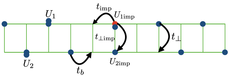
Figure 1: (color online) Impurity in a two-leg bosonic ladder. The blue solid circles represent the bath particles and the red circle represents the impurity. The bath particles move along the legs (resp. between the legs) with hopping $t_{b}$ (resp. $t_{\perp}$)(see text). The impurity moves in both longitudinal and transverse directions with amplitudes $t_{\text{imp}}$ and $t_{\perp\text{imp}}$ (see text) respectively. The impurity and the bath particles interact by the contact interactions $U_{1\text{imp}}$ and $U_{2\text{imp}}$ in leg 1 and leg 2 respectively.

The full Hamiltonian is given by

$$H=H_{K}+H_{\text{lad}}+U_{1\text{imp}}\sum_{j=1}^{L}\rho_{1,j}\rho_{\text{imp},1,j}$$ (1)

$$+U_{2\text{imp}}\sum_{j=1}^{L}\rho_{2,j}\rho_{\text{imp},2,j},$$

where $U_{1\text{imp}}$, $U_{2\text{imp}}$, and $L$ are the interactions strength between the particles in the leg 1, in the leg 2 with the impurity, and the ladder size along longitudinal direction, respectively. We consider $U_{1\text{imp}}=U_{2\text{imp}}=U_{b}$.

The impurity kinetic energy is given by the tight-binding Hamiltonian

$$H_{K}=-t_{\text{imp}}\sum_{j=1}^{L-1}(d^{\dagger}_{1,j+1}d_{1,j}+d^{\dagger}_{2,j+1}d_{2,j}+\text{h.c.})\\ -t_{\perp\text{imp}}\sum_{j=1}^{L}(d^{\dagger}_{1,j}d_{2,j}+\text{h.c.}).$$ (2)

We diagonalize $H_{K}$ by using symmetric and anti-symmetric combinations of $d_{1,j}$ and $d_{2,j}$, and $H_{K}$ can be re-expressed as

$$H_{\text{imp}}=\sum_{q}\epsilon_{s}(q)d^{\dagger}_{s,q}d_{s,q}+\epsilon_{a}(q)d^{\dagger}_{a,q}d_{a,q}$$ (3)

where $d_{\gamma,j}$ ($d^{\dagger}_{\gamma,j}$) are the destruction (creation) operators of the impurity on site $j$ in leg $\gamma=1,2$, $d_{s,q}=\frac{d_{1,q}+d_{2,q}}{\sqrt{2}},d_{a,q}=\frac{d_{1,q}-d_{2,q}}{\sqrt{2}}$, $\epsilon_{a}(q)=-2t_{\text{imp}}\cos(q)+t_{\perp\text{imp}}$, and $\epsilon_{s}(q)=-2t_{\text{imp}}\cos(q)-t_{\perp\text{imp}}$. The density of the impurity on site $j$ is

$$\rho_{\text{imp},1,j}=d^{\dagger}_{1,j}d_{1,j}.$$ (4)

The ladder Hamiltonian $H_{\text{lad}}$ is given by

$$H_{\text{lad}}=H^{0}_{1}+H^{0}_{2}-t_{\perp}\sum_{j=1}^{L}(b^{\dagger}_{1,j}b_{2,j}+\text{h.c.})$$ (5)

where $b_{a,j}$ ($b^{\dagger}_{a,j}$) are the destruction (creation) operators of a boson of the bath on chain $a$ and site $j$. The operators $b$ obey the usual commutation relation rules. The single chain Hamiltonian is the Bose-Hubbard one

$$H^{0}_{i}=-t_{b}\sum_{j=1}^{L-1}(b^{\dagger}_{i,j+1}b_{i,j}+\text{h.c.})+\frac{U_{i}}{2}\sum_{j=1}^{L}\rho_{i,j}(\rho_{i,j}-1)-\mu_{i}\sum_{j}\rho_{i,j}.$$ (6)

The eq. (1) is convenient for the numerical study. In order to make connection with the field theory analysis we can also consider the same problem in a continuum. In that case the Hamiltonian becomes

$$H=\frac{P^{2}}{2M}-t_{\perp\text{imp}}(|1\rangle\langle 2|+|2\rangle\langle 1|)\\ +H_{\text{lad}}+U(\rho_{1}(X)|1\rangle\langle 1|+\rho_{2}(X)|2\rangle\langle 2|),$$ (7)

where $X$ and $P$ are the position and momentum operators of the impurity.

The ladder Hamiltonian (5) in the continuum becomes as

$$H_{\text{lad}}=H^{0}_{1}+H^{0}_{2}-t_{\perp}\int dx(\psi^{\dagger}_{1}(x)\psi_{2}(x)+\text{h.c.}),$$ (8)

and the single chain Hamiltonian is

$$H^{0}_{i}=\frac{1}{2m}\int dx|\nabla\psi_{i}(x)|^{2}+\frac{U_{i}}{2}\int dx\rho_{i}(x)^{2}-\mu_{i}\int dx\rho_{i}(x),$$ (9)

where $m$ is the mass of the bosons, $\mu_{i}$ is the chemical potential and $U_{i}$ is the intrachain interaction.

II.2 Observables

To characterize the dynamics of the impurity in the ladder we mostly focus on the Green’s function of the impurity. We study it at zero temperature both analytically and numerically via DMRG. Compared to the case [9, 17] where the impurity was confined to a single chain, it is now necessary to introduce two independent Green’s functions for the impurity. The Green’s function are in the chain basis

$$G_{\alpha\beta}(p,t)=\langle\hat{d}_{\alpha,p}(t)\hat{d}_{\beta,p}^{\dagger}(t=0)\rangle,$$ (10)

where $\alpha$ and $\beta$ can take the values $1,2$ corresponding to the chain index and $\langle\cdots\rangle$ denotes the average in the ground state of the bath, and with zero impurities present. $O(t)$ denotes the usual Heisenberg time evolution of the operator

$$O(t)=e^{iHt}Oe^{-iHt},$$ (11)

and the operator $\hat{d}_{1p}$ is the operator destroying an impurity with momentum $p$ given by

$$\hat{d}_{1,p}=\sum_{j}e^{ipr_{j}}d_{1,j},$$ (12)

with $r_{j}=aj$ on the lattice and the corresponding integral

$$\hat{d}_{1,p}=\int dxe^{ipx}d_{1}(x),$$ (13)

in the continuum. By symmetry we can restrict ourselves to $G_{11}(p,t)$ and $G_{12}(p,t)$. The two other Green’s function are simply related to (10) by $G_{22}(p,t)=G_{11}(p,t)$ and $G_{12}(p,t)=G_{21}(p,t)$,

Instead of using the chain basis it can be more convenient to use the symmetric $s$ and antisymmetric $a$ operators leading to the two Green’s functions

$$\begin{split}G_{s}(p,t)&=\langle\hat{d}_{s,p}(t)\hat{d}_{s,p}^{\dagger}(t=0)\rangle,\\ G_{a}(p,t)&=\langle\hat{d}_{a,p}(t)\hat{d}_{a,p}^{\dagger}(t=0)\rangle,\end{split}$$ (14)

all other combinations being zero by symmetry. One has $G_{s}(p,t)=G_{11}(p,t)+G_{12}(p,t)$, $G_{a}(p,t)=G_{11}(p,t)-G_{12}(p,t)$.

II.3 Bosonization representation

To deal with the Hamiltonian defined in the previous section, we use the fields $\theta_{\alpha}(x)$ and $\phi_{\alpha}(x)$  [9] for chain $\alpha=1,2$ which are related to the field operators of the system via

$$\rho_{\alpha}(x)=\rho_{0,\alpha}-\frac{\nabla\phi_{\alpha}(x)}{\pi}+\rho_{0}\sum_{p\neq 0}e^{2ip(\pi\rho_{0,\alpha}x-\phi_{\alpha}(x))},$$ (15)

where $\rho_{0,\alpha}$ is the average density on the chain $\alpha=1,2$. The creation operator of a particle in the bath in term of $\theta$ and $\phi$ is given to lowest order by

$$\psi_{\alpha}^{\dagger}(x)=\rho_{0,\alpha}^{1/2}e^{-i\theta_{\alpha}(x)}.$$ (16)

The conjugate field operators $\phi_{1,2}$ and $\theta_{1,2}$ obeys

$$[\phi(x_{1}),\frac{\nabla\theta(x_{2})}{\pi}]=i\delta(x_{1}-x_{2}).$$ (17)

Using the bosonization framework, the Hamiltonian of the ladder is given by

$$H_{\text{lad}}=H_{s}+H_{a},$$ (18)

with

$$\begin{split}H_{s}=&\frac{1}{2\pi}\int dx[u_{s}K_{s}(\partial_{x}\theta_{s})^{2}+\frac{u_{s}}{K_{s}}(\partial_{x}\phi_{s})^{2}],\\ H_{a}=&\frac{1}{2\pi}\int dx[u_{a}K_{a}(\partial_{x}\theta_{a})^{2}+\frac{u_{a}}{K_{a}}(\partial_{x}\phi_{a})^{2}]\\ &-2\rho_{0}t_{\perp}\int dx\cos(\sqrt{2}\theta_{a}(x)),\end{split}$$ (19)

and

$$\begin{split}\theta_{s,a}=&\frac{\theta_{1}\pm\theta_{2}}{\sqrt{2}},\\ \phi_{s,a}=&\frac{\phi_{1}\pm\phi_{2}}{\sqrt{2}}.\end{split}$$ (20)

The cosine term [9, 17] opens a gap in the antisymmetric sector when $K_{a}>1/4$. This massive phase for the antisymmetric phase excitations signals the existence of phase coherence across the two legs of the ladder, with exponentially decreasing correlations for the antisymmetric density-density correlations. The symmetric sector is described by the usual TLL Hamiltonian, and has powerlaw correlations. A numerical calculation of the TLL parameters for the massless phase can be found in [30].

III Analytical solution for weak coupling

Let us now investigate the full Hamiltonian (7) (or (1)) to compute the Green’s function of the impurity (10).

Using (15) the interaction term $H_{\text{coup}}$ with the impurity in terms of the $d_{s}$ and $d_{a}$ becomes

$$H_{\text{coup}}=\frac{U}{2}\int dx(\rho_{1}(x)+\rho_{2}(x))(d_{s}(x)^{\dagger}d_{s}(x)+d_{a}(x)^{\dagger}d_{a}(x))\\ +\frac{U}{2}\int dx(\rho_{1}(x)-\rho_{2}(x))(d_{s}(x)^{\dagger}d_{a}(x)+h.c),$$ (21)

which leads to the expression, in terms of the symmetric and anti-symmetric modes of the bath,

$$H_{\text{coup}}=\frac{-U}{\sqrt{2}\pi}\int dx\nabla\phi_{s}(x)(d_{s}(x)^{\dagger}d_{s}(x)+d_{a}(x)^{\dagger}d_{a}(x))\\ -\frac{U}{\sqrt{2}\pi}\int dx\nabla\phi_{a}(x)(d_{s}(x)^{\dagger}d_{a}(x)+h.c).$$ (22)

Note that we have kept in (22) only the most relevant term, which for bosons is the forward scattering on the symmetric and anti-symmetric modes of the bath.

To compute the Green’s functions We use same approach as in [17], namely the linked cluster expansion (LCE) [24, 10, 31]. The calculation is detailed in Appendix A and gives the asymptotic behavior of the impurity Green’s function (10) for $2t_{\perp\text{imp}}>\frac{\Delta_{a}\sqrt{2u_{a}\pi}}{\sqrt{K_{a}}}$ as

$$\begin{split}|G_{s}(p,t)|&=e^{-\frac{K_{s}U_{s}^{2}}{4\pi^{2}u_{s}^{2}}(1+\frac{12t_{\text{imp}}^{2}p^{2}}{u_{s}^{2}})\log(t)},\\ |G_{a}(0,t)|&=e^{-aU_{a}^{2}t}\end{split}$$ (23)

where $K_{s}=.835$, $u_{s}=1.86$ for $t_{b}=t_{\perp}=1,U_{1}=U_{2}=\infty,\rho_{0}=1/3$ [30] and

$$a \simeq\frac{K_{a}}{4u_{a}\pi^{2}}\frac{(u_{a}^{2}q_{-}^{2}+\tilde{\Delta}^{2})}{q_{-}(2t_{\text{imp}}\sqrt{u_{a}^{2}q_{-}^{2}+\tilde{\Delta}^{2}}+u_{a}^{2})},$$ (24)

where $q_{-}$ and $\tilde{\Delta}$ are expressed in A. In our LCE calculation we also finds that for $2t_{\perp\text{imp}}<\frac{\Delta_{a}\sqrt{2u_{a}\pi}}{\sqrt{K_{a}}}$ the Green’s function in both symmetric and anti-symmetric sectors decay as a power-law at $p=0$. However, the Green’s functions of the impurity at $p=0$ in two-decoupled chains [18] always decay as power-law and exponentially in the symmetric and anti-symmetric sector at any finite transverse tunneling of the impurity, respectively. For this case, one needs to choose a sufficiently small $t_{\perp\text{imp}}$. However, to compare the LCE with the t-DMRG results, we need to wait for a longer time for which the impurity will realize the effect of the $t_{\perp\text{imp}}$. Such time is inaccessible in t-DMRG because of the entanglement growth in the system with time, which is often linear [32]. So, in order to compare t-DMRG results with LCE, we chose a sufficiently large $t_{\perp\text{imp}}$ in our work. For a weak repulsion between the impurity and the bath we thus find that the Green’s function in the symmetric mode decays as a power-law with time as was the case with an impurity confined to a single chain [17]. In the anti-symmetric mode on the other hand it decays exponentially.

IV Numerical solution

Analyzing the regime $U\gg\Delta_{a}$ is much more involved since now excitations across the antisymmetric gap can be created. We thus turn to a numerical analysis of this problem.

IV.1 Method

We use time-dependent DMRG (t-DMRG) [32] to compute the Green’s function of the impurity, and we follow the method described in Ref. [31, 17, 33]. For completeness let us recall the method, which is described below.

We map the ladder-impurity problem to a one-dimensional problem by a supercell approach. We denote bath particles in leg 1 and leg 2 by $B$ and $C$, the impurity in leg 1 and leg 2 by $A$ and $D$ and the total number of bath particles and number of impurity are conserved separately. The local dimension of Hilbert space for A, B, C, D is two for hardcore bosons hence the dimension of local Hilbert space of supercell (A, B, C, D) is $2\times 2\times 2\times 2=16$. We compute the Green’s function of the impurity in the ground state of the ladder . The ground state $(|GS_{b}\rangle)$ is computed using DMRG. The Green’s functions $G_{11}(x,t)(G_{12}(x,t))$ of the impurity in Heisenberg picture is given by

$$G_{11}(x,t)=e^{iE_{GS_{b}}t}\langle GS_{b}|d_{1,\frac{L+1}{2}-x}e^{-iHt}d^{\dagger}_{1,\frac{L+1}{2}}|GS_{b}\rangle,$$

$$G_{12}(x,t)=e^{iE_{GS_{b}}t}\langle GS_{b}|d_{2,\frac{L+1}{2}-x}e^{-iHt}d^{\dagger}_{1,\frac{L+1}{2}}|GS_{b}\rangle,$$ (25)

where $E_{GS_{b}}$ is ground state energy of the bath. We compute $e^{-iHt}d^{\dagger}_{1,\frac{L+1}{2}}|GS_{b}\rangle$ using t-DMRG and $\langle GS_{b}|d_{2,\frac{L+1}{2}-x}$$(\langle GS_{b}|d_{1,\frac{L+1}{2}-x})$ are computed using DMRG. By using $G_{11}(x,t)$ and $G_{12}(x,t)$, we compute $G_{s}(x,t)=G_{11}(x,t)+G_{12}(x,t)$ and $G_{a}(x,t)=G_{11}(x,t)-G_{12}(x,t)$. For the numerical calculation we have used a bath of hardcore bosons at a density of $\rho_{0}=1/3$. This choice avoids the Mott-insulating phase that the ladder’s symmetric mode might enters at commensurate density [30]. We have used a bond dimension $\chi=400$ to compute the Green’s function in a reasonable time. We chose Hamiltonian parameters $t_{\perp}=t_{b}=t_{\text{imp}}=1,U_{1}=U_{2}=\infty$ and various values of $t_{\perp\text{imp}}$ and $U$. We fix the size of the system to $L=101$ sites per leg.

IV.2 Zero momentum regime

We show the Green’s function of the impurity in the anti-symmetric and symmetric modes $|G_{a}(p,t)|,|G_{s}(p,t)|$ at momentum $p=0$ in Fig. 2 on semi-log and log-log scales, we find that $|G_{s}(0,t)|$ decays as a power-law which is similar to one observed in one-dimensional motion of the impurity in a two-leg bosonic ladder [17]. However, the Green’s function of the impurity in the anti-symmetric mode shows an exponential decay.

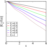
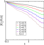
Figure 2: (color online) The modulus of the green’s function of the impurity in anti-symmetric (left panel) and symmetric sectors (right panel) as a function of time for hardcore bosonic bath at $t_{\text{imp}}=t_{\text{b}}=1$, $\text{t}_{\perp}=1$, $\text{U}=0.5-1$, $t_{\perp\text{imp}}=3$ and $\text{p}=0$. The left panel is depicted on semi-log scale show a linear behavior while right panel shows a linear behavior on log-log scale.

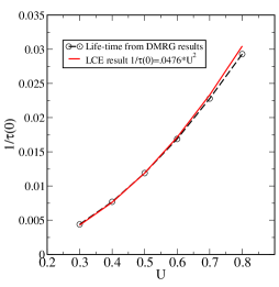
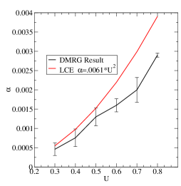
Figure 3: (color online) Life-time of the impurity in anti-symmetric sector (upper panel) and power-law exponent (lower panel) in the symmetric at $t_{\text{imp}}=t_{\text{b}}=1$, $\text{t}_{\perp}=1$, $t_{\perp\text{imp}}=3$ as function of $U$ at zero momentum. The black lines are numerical results and the red lines are LCE results, both numerical and analytical results show a nice agreement for small $U$.

For the parameters used in these two figures the gap in the antisymmetric sector is $\Delta_{a}=.33t_{b}$. This value of the impurity-bath interaction corresponds to the regime of weak coupling for which a comparison with the analytical results of Sec. III is meaningful. The comparison of the numerical results with the analytical results (23) is shown in Fig. 3. The numerical analysis thus fully confirms that in this regime the $G_{s}(0,t)$ and $G_{a}(0,t)$ decay as power-law and exponentially, respectively. To further analyze the data we fit the numerical results to the form

$$\begin{split}|G_{a}(p=0,t)|\propto\exp(-t/\tau(0))\\ |G_{s}(p=0,t)|\propto\left(\frac{1}{t}\right)^{\alpha}\end{split}$$ (26)

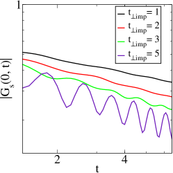
Figure 4: (color online) Modulus of the Green’s function of the impurity (see text) $|G_{s}(p,t)|$ at momentum $p=0$ for the impurity. Parameters for the intra-chain hopping, inter-chain hopping (for the ladder), impurity hopping, impurity interaction, impurity transverse tunneling in the ladder are respectively $t_{b}=1$, $t_{\perp}=1$, $t_{\text{imp}}=1$, $t_{\perp\text{imp}}=1,2,3,5$, and $U=\infty$.

IV.2.1 Small U

To analyze the data, we use the analytic estimates of Sec. III which suggest a power law and an exponential decay of the Green’s function of the symmetric and the anti-symmetric mode respectively.

We fit the numerical data with the linked cluster expansion (LCE) result at $p=0$ and they agree very well with numerical results. The numerical and analytical results for $G_{a}$ and $G_{s}$ are shown in Fig. 3.

IV.2.2 Hardcore bath-impurity repulsion

In the case of $U\to\infty$, $|G_{s}(p,t)|$ is plotted on the log-log scale in Fig. 4 for different value of $t_{\perp\text{imp}}$ at $p=0$. As shown, $|G_{s}(p,t)|$ decays as a power-law and the power-law exponent as function of $t_{\perp\text{imp}}$ is depicted in Fig. 5.

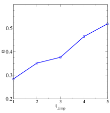
Figure 5: (color online) Power-law exponent of the symmetric Green’s function of the impurity with a hardcore repulsion with the bath of hardcore bosons at filling $1/3$ as a function of $t_{\perp\text{imp}}$ at $t_{\text{imp}}=1$, $U\rightarrow\infty$ and p=0. Circles are the numerical data for $\chi=400$ and the line is a guide to the eyes.

The power-law exponent increases as a function of $t_{\perp\text{imp}}$. For a small $t_{\perp\text{imp}}$, the exponent is similar to the one observed for the purely one-dimensional motion of an impurity in a two-leg ladder bath [17], while for a large $t_{\perp\text{imp}}$, it is similar to the motion of an impurity in a one-dimensional bath  [14, 29].

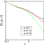
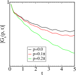
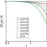
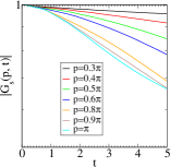
Figure 6: (color online) Modulus of the Green’s function of the impurity in the symmetric sector (see text) $|G_{s}(p,t)|$ at different momentum $p$ (c.f. legend) for the impurity. The Hamiltonian parameters are $t_{b}=1$, $t_{\perp}=1$, $t_{\text{imp}}=1$, $t_{\perp\text{imp}}=3$ and $U=1.0$ on log-log scale (right panel) and semi-log scale (left panel) . We observe a linear behavior on log-log scale for small momenta ($\text{p}=0-0.2\pi$), and linear behavior for large momenta $\text{p}=0.3\pi-\pi$ on semi-log scale.

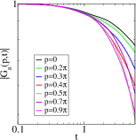
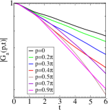
Figure 7: Modulus of the Green’s function of the impurity in ant-symmetric sector (see text) $|G_{a}(p,t)|$ at different momentum $p$ (shown in inset) for the impurity. The Hamiltonian parameters are $t_{b}=1$, $t_{\perp}=1$, $t_{\text{imp}}=1$, $t_{\perp\text{imp}}=3$ and $U=1.0$ on log-log scale (right panel) and semi-log scale (left panel) . We observe a linear behavior on semi-log scale for all momenta ($\text{p}=0-0.9\pi$).

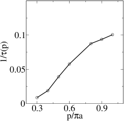
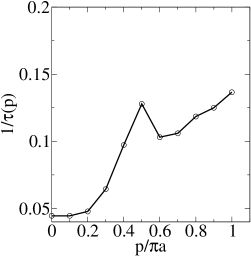
Figure 8: Inverse life-time of the impurity in both symmetric (upper panel) and anti-symmetric (lower panel) sectors as function of momentum at $t_{b}=1$, $t_{\perp}=1$, $t_{\text{imp}}=1$, $t_{\perp\text{imp}}=3$ and $U=1.0$.

IV.3 Green’s function at finite momentum

As we have seen previously that the Green’s function decays as a power-law in the symmetric mode and exponentially in the anti-symmetric mode at $p=0$, now we turn on finite momentum. The Green’s functions $|G_{s}(p,t)|$ and $|G_{a}(p,t)|$ for finite momentum are shown in Fig. 6 and 7, respectively, for various momenta $p$ of the impurity. We find that $|G_{s}(p,t)|$ decays as power-law below $p=0.3\pi$ and beyond $p=0.3\pi$. Beyond this point, it decays exponentially and the impurity in the symmetric mode enters into a QP regime. An analogus crossover has been established in the one-dimensional motion of an impurity in a one-dimensional bath  [31] and two-leg bosonic ladder bath [17, 33].

The crossover depends on the TLL characteristics of the bath in the symmetric sector, namely the velocity of sound $u_{s}$ in the ladder and the TLL parameter $K_{s}$. Using the values extracted from [30] we get

$$p^{*}=\frac{u_{s}}{2t_{b}}=.93$$ (27)

which is in reasonably good agreement with the observed change of behavior in Fig. 6.

Beyond $\text{p}=\text{p}^{*}$ and for small $U$, the Green’s function decays exponentially, the impurity behaves like a QP and the Green’s function of the impurity in term of life time $\tau(p)$ is given by

$$\begin{split}|G_{s}(p,t)|&=\exp(-t/\tau(p))\end{split}$$ (28)

In the top panel of the Fig. 8, we plot the inverse of life time $1/\tau(p)$ in the symmetric mode of the impurity, defined in eq. (28) of the QP as function of p for interaction $U=1,t_{\perp\text{imp}}=3$. As can be expected $1/\tau(p)$ increases with increasing p.

In Fig. 7, we have shown $|G_{a}(p,t)|$ on semi-log and log-log scales, we find that the $|G_{a}(p,t)|$ always decays as exponentially for all momenta, and the impurity in the anti-symmetric band always behaves like a QP. In the bottom panel of the Fig. 8, we have shown the inverse lifetime as a function $p$, it shows a non-monotonic behavior but overall increases with increasing $p$.

V Discussion

Our findings suggest that the impurity exhibits a very different dynamics in the ladder because of the motion in the horizontal and transverse directions than ones observed in one-dimensional (1D) motion of an impurity in a ladder and 1D bath.

Let us first discuss the weak interaction limit. Initially, both the symmetric and anti-symmetric modes of the impurity couple to both gapless and gapped mode of the bath, but our numerical and analytical findings suggest that in the long-time limit the impurity in the anti-symmetric sector effectively couples to the gapped mode of the bath and the impurity in the symmetric mode couples to the gapless mode of the bath with an effective interaction $U/\sqrt{2}$. Both the numerical and analytical results show an excellent agreement as depicted in Fig. 2 and 3.

The transverse tunneling of the impurity is the main ingredient in the exponential decay of the Green’s function of the impurity in the anti-symmetric mode while for the Green’s function in the symmetric mode, the power-law exponent does not depend on the transverse tunneling of the impurity.

Now let us turn to infinite interaction limit between the impurity and the bath. We find that the Green’s function in the symmetric sector decays as a power law at zero momentum, which is similar to the one observed in the impurity dynamics in a one-dimensional (1D) bath and two-leg ladder bath. However, the power-law exponent increases with the tunneling amplitude of the impurity which is contrasted the one observed for small $U$, where power-law exponent does not depend on $t_{\perp\text{imp}}$. We find that for small $t_{\perp\text{imp}}$, the power-law exponent is same as the one observed in 1D motion in the ladder bath but for larger value the power law exponent is equal to one observed in the 1D bath. As a function of $t_{\perp\text{imp}}$, we observed that the impurity dynamics exhibits a dimensional crossover from ladder to 1D bath. For large transverse tunneling, one can understand that the impurity will energetically favor the symmetric mode of the impurity, and it would be hard to excite the impurity from symmetric to anti-symmetric mode and vice versa. Hence the impurity effectively moves in a gapless 1D bath formed by the ladder’s symmetric mode. This description contradicts our common understanding that in a ladder the power-law exponent should be smaller than that of 1D motion in the ladder [17].

It will be interesting to investigate how the dynamics of the impurity behaves with increasing the number of legs and this needs a further study.

Our findings also suggest that the impurity in the symmetric sector at the zero momentum in the ladder can be viewed as an X-ray edge problem [9]. The Green’s function in the X-ray edge problem has similar behaviour as the Green’s function of the symmetric mode at zero momentum. Of course in this case, contrarily to the historical X-ray edge problem the impurity can move. At zero longitudinal tunneling of the impurity the impurity-ladder problem can be mapped into a spin-boson problem [4] and by using an unitary transformation it can also be mapped into a Kondo problem [34]. The impurity-ladder problem can be viewed as a quantum simulator for the spin-boson model and Kondo problem.

Now we finally turn to the case of finite momentum. For small interaction and small momentum, the Green’s functions in the symmetric mode of the impurity decay as a power-law which are shown in the upper panel of the Fig. 6 . Beyond a critical momentum $\text{p}^{\ast}$, the Green’s function is depicted in the lower panel of the Fig. 6, it decays exponentially, and the impurity enters into a QP regime which is very similar to ones observed in the 1D motion of an impurity in a one-dimensional bath and in a two-leg bosonic ladder when $t_{\perp\text{imp}}$ is zero. The critical momentum is precisely equal to that of 1D motion of an impurity in a ladder and in a 1D bath. The Green’s functions of the impurity in the anti-symmetric mode are depicted in Fig. 7, and they always decay exponentially for all momenta, and the impurity in the anti-symmetric mode always behave like a QP.

VI Conclusion and perspectives

We have studied the dynamics of an impurity in a reservoir of hard-core bosons moving in a two-leg ladder where the impurity may tunnel in both transverse and horizontal directions. We have computed the Green’s function of the impurity for different momenta in order to understand the dynamics of the impurity. We use both analytical and numerical approaches, where later are comprised of the time-dependent DMRG.

When impurity-bath interactions are weak, the Green’s function of the impurity in the symmetric sector decays as a power-law below a critical momentum and exponentially above the critical momentum like the 1D dynamics of an impurity in a two-leg ladder bath where transverse tunneling of the impurity is suppressed. However, in the anti-symmetric sector the Green’s function of the impurity always decays exponentially and the impurity behaves like a quasi-particle. One can expect that when the bath is made of several 1D chains then in the lowest energy band of the impurity, the impurity would exhibit a crossover (beyond a critical momentum) from a power-law to an exponential decay. However, in the other energy sectors of the impurity, the Green’s function would decay exponentially.

The above observations suggest that the crossover of the dynamics of the impurity from a one-dimensional bath to a two-dimensional bath made up of finite number of 1D baths is not smoothly connected.

The system we have studied can be tested experimentally in the context of circuit QED  [35, 36] and cold atoms. When the impurity moves only in transverse direction, the impurity acts like a two-level system which is analogous to a supercondcting qubit, and the two-leg ladder bath acts like a one-dimensinal wave guide, and the impurity-reservoir interaction is the equivalent of the standard qubit-waveguide coupling. The bosonic ladder has been realized experimentally in ultracold gasses  [37, 38] and atom chips [39] .The impurity dynamics in one-dimensional bath has been investigated experimentally using ultracold gasses [20, 21, 22, 23]. Combination of these aspects and ongoing experimental advancement in the ultracold gasses could provide the ideal testbed for our findings in near future.

Appendix A Green’s function of the mobile impurity in the two-leg bosonic Ladder

As we have shown in the main text (see section III) that for small interaction $U$ between the impurity and the ladder bath the impurity effectively coupled to the forward scattering terms of the gapped and gapless modes of the bath.

In this section, we give a linked-cluster expansion (LCE) expression of the Green’s function of the impurity. We express $\cos(\sqrt{2}\theta_{a})=1-\theta_{a}^{2}$ and use the continuity equation

$$\nabla\phi_{a}(q,t)=\frac{\partial\theta_{a}(q,t)}{\partial t}.$$ (29)

The impurity-bath Hamiltonian is expressed as

$$\begin{split}H&=H_{s}+H_{a}+H_{\text{imp}}+H_{\text{coup}},\end{split}$$ (30)

where $H_{\text{s}}$, $H_{\text{a}}$, $H_{\text{imp}}$, and $H_{\text{coup}}$ are the symmetric mode, anti-symmetric mode of the bath, the impurity Hamiltonian, and the coupling between the impurity and the bath, respectively, and these terms in bosonized language are expressed as

$$\begin{split}H_{s}&=\sum_{q}u_{s}|q|b^{\dagger}_{s,q}b_{s,q},\\ H_{a}&=\frac{1}{2\pi}\int dx\Big{[}u_{a}K_{a}(\partial_{x}\theta_{a})^{2}+\frac{u_{a}}{K_{a}}(\partial_{x}\phi_{a})^{2}\Big{]}\\ &-\Delta_{a}^{2}\int dx\theta(x)^{2},\\ H_{\text{coup}}&=\sum_{{q},{k}}\Big{[}V(q)(d^{\dagger}_{s,{k}+{q}}d_{s,{k}}+d^{\dagger}_{a,{k}+{q}}d_{a,{k}})(b_{{s,q}}+b^{\dagger}_{{s,-q}})\\ &+\tilde{U}(d^{\dagger}_{a,{k}+{q}}d_{s,{k}}+d^{\dagger}_{s,{k}+{q}}d_{a,{k}})\frac{\partial\theta_{a}(q,t)}{\partial t}\Big{]},\\ H_{\text{imp}}&=\sum_{q}\epsilon_{s}(q)d^{\dagger}_{s,q}d_{sq}+\epsilon_{a}(q)d^{\dagger}_{a,q}d_{a,q},\end{split}$$ (31)

where $\tilde{U}=-\frac{U}{\sqrt{2}\pi}$, $b^{\dagger}$ and $d^{\dagger}$ are the creation operators for the bath in the bosonized language and the impurity respectively, $\epsilon_{a}(p)=-2t_{\text{imp}}\cos(p)+t_{\perp\text{imp}}$, $\epsilon_{s}(p)=-2t_{\text{imp}}\cos(p)-t_{\perp\text{imp}}$. $\Delta_{a}$ is the gap in the anti-symmetric mode of the bath. The coupling term $V(q)$ can be expressed as

$$V(q) = \frac{U}{\sqrt{2}}\sqrt{\frac{K_{s}|q|}{2\pi L}}\exp\Big{(}-\frac{|q|}{2q_{c}}\Big{)}.$$ (32)

The Green’s function of the impurity in symmetric and ant-symmetric sectors are defined by

$$\begin{split}G_{s}(p,t)&=-i\langle d_{s,p}(t)d^{\dagger}_{s,p}(0)\rangle,\\ G_{a}(p,t)&=-i\langle d_{a,p}(t)d^{\dagger}_{a,p}(0)\rangle.\end{split}$$ (33)

By using LCE, (33) can be written as

$$G_{s}(p,t) = -{i}e^{-i\epsilon_{s}(p)t}e^{F_{2s}(p,t)},$$

$$G_{a}(p,t) = -{i}e^{-i\epsilon_{a}(p)t}e^{F_{2a}(p,t)},$$ (34)

where $F_{2,s/a}(p,t)$ is defined as

$$F_{2s/a}(p,t) = e^{i\epsilon_{s/a}(p)t}W_{2s/a}(p,t).$$ (35)

$W_{2s/a}(p,t)$ is given by

$$W_{2s/a}(p,t) = -\frac{1}{2}\int_{0}^{t}dt_{1}\int_{0}^{t}dt_{2}$$

$$\times\langle T_{t}d_{s/a,p}(t)H_{\text{coup}}(t_{1})H_{\text{coup}}(t_{2})d^{\dagger}_{s/a,p}(0)\rangle.$$

By employing the Wick’s theorem $W_{2a}(p,t)$ can be expressed as

$$W_{2a}(p,t) =-\sum_{q}\int_{0}^{t}dt_{1}\int_{0}^{t}dt_{2}Y(t-t_{1})Y(t_{1}-t_{2})$$ (37)

$$\times Y(t_{2})\Big{[}V(q)^{2}e^{-i\epsilon_{a}(p)(t-t_{1})}e^{-i\epsilon_{a}(p+q)(t_{1}-t_{2})}$$

$$\times e^{-i\epsilon_{a}(p)t_{2}}e^{-i(u_{a}|q|(t_{1}-t_{2}))}$$

$$+\frac{U_{a}^{2}}{4\pi}\sqrt{K_{a}^{2}q^{2}+\frac{2\pi\Delta_{a}^{2}K_{a}}{u_{a}}}e^{-i\epsilon_{a}(p)(t-t_{1})}$$

$$\times e^{-i\epsilon_{s}(p+q)(t_{1}-t_{2})}e^{-i\epsilon_{a}(p)t_{2}}$$

$$\times e^{-i\Big{(}\sqrt{u_{a}^{2}q^{2}+\frac{2\pi\Delta_{a}^{2}u_{a}}{K_{a}}}(t_{1}-t_{2})\Big{)}}\Big{]},$$

where $Y(t)$ is a step function, which is zero for $t<0$ and one for $t>0$. $U_{a}$ is coupling between the impurity and the anti-symmetric mode of the bath, at this moment $U_{a}=U$. $Y(t)$ changes the limit of integration of $t_{2}$ and $t_{1}$, and $F_{2a}(p,t)$ is modified as

$$F_{2a}(p,t) =-\sum_{q}\int_{0}^{t}dt_{1}\int_{0}^{t_{1}}dt_{2}\Big{[}V(q)^{2}e^{i\epsilon_{a}(p)t_{1}}e^{-i\epsilon_{a}(p+q)(t_{1}-t_{2})}$$

$$\times e^{-i\epsilon_{a}(p)t_{2}}e^{-i(u_{a}|q|(t_{1}-t_{2}))}+\frac{U_{a}^{2}}{4\pi}$$

$$\times\sqrt{K_{a}^{2}q^{2}+\frac{2\pi\Delta_{a}^{2}K_{a}}{u_{a}}}e^{i\epsilon_{a}(p)t_{1}}e^{-i\epsilon_{s}(p+q)(t_{1}-t_{2})}$$

$$\times e^{-i\epsilon_{a}(p)t_{2}}e^{-i\Big{(}\sqrt{u_{a}^{2}q^{2}+\frac{2\pi\Delta_{a}^{2}u_{a}}{K_{a}}}(t_{1}-t_{2})\Big{)}}\Big{]}.$$ (38)

We can simplify eq. (A) as

$$\begin{split}F_{2a}(p,t)&=-\sum_{q}\int du\int_{0}^{t}dt_{1}\int_{0}^{t_{1}}dt_{2}\\ &\times\Big{[}V(q)^{2}e^{it_{1}u}e^{-it_{2}u}\delta(u-\epsilon(p)+\epsilon(p+q)+u_{a}|q|)\\ &+\frac{U_{a}^{2}}{4\pi}\sqrt{K_{a}^{2}q^{2}+\frac{2\pi\Delta_{a}^{2}K_{a}}{u_{a}}}e^{-it_{1}(u-2t_{\perp\text{imp}})}e^{it_{2}(u-2t_{\perp\text{imp}})}\\ &\times\delta\Big{(}u+\epsilon(p)-\epsilon(p+q)-\sqrt{u_{a}^{2}q^{2}+\frac{2\pi\Delta_{a}^{2}K_{a}}{u_{a}}}\Big{)}\Big{]}.\end{split}$$ (39)

Finally, we integrate over $t_{1}$ and $t_{2}$ and the real part of $F_{2a}$ can be expressed as

$$\begin{split}\text{Re}[F_{2a}(p,t)]&=-\sum_{q}\int du\Big{[}V(q)^{2}\frac{(1-\cos(ut))}{u^{2}}\\ &\times\delta(u-\epsilon(p)+\epsilon(p+q)+u_{a}|q|)\\ &+\frac{U_{a}^{2}}{4\pi}\sqrt{K_{a}^{2}q^{2}+\frac{2\pi\Delta_{a}^{2}K_{a}}{u_{a}}}\frac{(1-\cos(t(u-2t_{\perp\text{imp}})))}{(u-2t_{\perp\text{imp}})^{2}}\\ &\times\delta(u+\epsilon(p)-\epsilon(p+q)-\sqrt{u_{a}^{2}q^{2}+\frac{2\pi\Delta_{a}^{2}K_{a}}{u_{a}}})\Big{]}.\end{split}$$ (40)

Similarly one can show that

$$\begin{split}\text{Re}[F_{2s}(p,t)]&=-\sum_{q}\int du\\ &\times\Big{[}V(q)^{2}\delta(u-\epsilon(p)+\epsilon(p+q)+u_{s}|q|))\\ &\times\frac{(1-\cos(ut))}{u^{2}}+\frac{U_{a}^{2}}{4\pi}\sqrt{K_{a}^{2}q^{2}+\frac{2\pi\Delta_{a}^{2}K_{a}}{u_{a}}}\\ &\times\frac{(1-\cos(t(u+2t_{\perp\text{imp}})))}{(u+2t_{\perp\text{imp}})^{2}}\\ &\times\delta\Big{(}u+\epsilon(p)-\epsilon(p+q)-\sqrt{u_{a}^{2}q^{2}+\frac{2\pi\Delta_{a}^{2}u_{a}}{K_{a}}}\Big{)}\Big{]},\\ &=-\int du\Big{[}\frac{(1-\cos(ut))}{u^{2}}R_{1s}(u,p)\\ &+\frac{(1-\cos(t(u+2t_{\perp\text{imp}})))}{(u+2t_{\perp\text{imp}})^{2}}R_{2}(u,p)\Big{]}.\end{split}$$ (41)

$R_{1s/a}(u)$ and $R_{2}$ are expressed as

$$\begin{split}R_{1s/a}(u,p)&=\frac{1}{2\pi}\int dqV(q)^{2}\\ &\times\delta(u-(\epsilon(p)-\epsilon(p+q)-u_{s/a}|q|)),\\ \end{split}$$ (42)

$$\begin{split}R_{2}(u,p)&=\frac{U_{a}^{2}}{8\pi^{2}}\int dq\sqrt{K_{a}^{2}q^{2}+\frac{2\Delta_{a}^{2}K_{a}\pi}{u_{a}}}\\ &\times\delta\Big{(}u+\epsilon(p)-\epsilon(p+q)-\sqrt{u_{a}^{2}q^{2}+\frac{\Delta_{a}^{2}u_{a}2\pi}{K_{a}}}\Big{)}.\end{split}$$ (43)

For small $p$, $\epsilon(p)\simeq 2t_{{\mbox{\scriptsize imp}}}p^{2}$ . $R_{1}(u,p)$ is computed in Ref. [31, 17] for $(p-\frac{u_{s}}{2t_{\text{imp}}})<0,\wedge u<0$. However, the computation of $R_{2}(u,p)$ for an arbitrary $p$ is difficult analytically so we restrict at $p=0$. At $p=0$, $R_{1}$ is non-zero for $u<0$ can be expressed as

$$R_{1s/a}(u,0) \propto u,$$ (44)

and for $u>0$

$$R_{2}(u,0) \propto A_{2}.$$ (45)

Let us define $A_{s}(u,t)$ and $A_{a}(u,t)$ as

$$\begin{split}A_{a}(u,t)&=\int_{0}^{\infty}du\Big{[}\frac{1-\cos(ut)}{u}\Big{]}\\ &+\int_{\frac{\Delta_{a}\sqrt{2u_{a}\pi}}{\sqrt{K_{a}}}-2t_{\perp\text{imp}}}^{\infty}du\Big{[}\frac{1-\cos(ut)}{u^{2}}A_{2}\Big{]},\\ A_{s}(u,t)&=\int_{0}^{\infty}du\Big{[}\frac{1-\cos(ut)}{u}\Big{]}\\ &+\int_{\frac{\Delta_{a}\sqrt{2u_{a}\pi}}{\sqrt{K_{a}}}+2t_{\perp\text{imp}}}^{\infty}du\Big{[}\frac{1-\cos(ut)}{u^{2}}A_{2}\Big{]}.\end{split}$$ (46)

In the long time limit $A_{s}$ and $A_{a}$ can be expressed as

$$\begin{split}A_{a}(u,t)&\simeq A_{2}\pi t,\\ A_{s}(u,t)&\simeq-\log(t),\end{split}$$ (47)

where $A_{2}$ is expressed as

$$A_{2}\simeq\frac{U^{2}K_{a}}{4u_{a}\pi^{2}}\frac{(u_{a}^{2}q_{-}^{2}+\tilde{\Delta}^{2})}{q_{-}(2t_{\text{imp}}\sqrt{u_{a}^{2}q_{-}^{2}+\tilde{\Delta}^{2}}+u_{a}^{2})},$$ (48)

and $\tilde{\Delta}$ and $q_{-}$ are expressed as

$$\begin{split}\tilde{\Delta}&=\frac{\Delta_{a}\sqrt{u_{a}2\pi}}{\sqrt{K_{a}}},\\ q_{-}&=\sqrt{\frac{2t_{\perp\text{imp}}}{t_{\text{imp}}}+\frac{u_{a}^{2}}{2{t_{\text{imp}}^{2}}}-\sqrt{\Big{(}\frac{2t_{\perp\text{imp}}}{t_{\text{imp}}}+\frac{u_{a}^{2}}{2{t_{\text{imp}}}^{2}}\Big{)}^{2}-\frac{(4t_{\perp\text{imp}}^{2}-\tilde{\Delta}^{2})}{t_{\text{imp}}^{2}}}}.\end{split}$$ (49)

By using equations (40, 41, 46, 47), the final expression of $F_{2s},F_{2a}$ for $2t_{\perp\text{imp}}>\frac{\Delta_{a}\sqrt{2u_{a}\pi}}{\sqrt{K_{a}}}$ in long-time limit is given by

$$\text{Re}[F_{2a}(0,t)] \simeq -A_{2}\pi t$$ (50)

$$\text{Re}[F_{2s}(0,t)] \simeq -\log(t)$$ (51)

For $2t_{\perp\text{imp}}<\frac{\Delta_{a}\sqrt{2u_{a}\pi}}{\sqrt{K_{a}}}$

$$\text{Re}[F_{2a}(0,t)] \simeq -\log(t)$$ (52)

$$\text{Re}[F_{2s}(0,t)] \simeq -\log(t)$$ (53)

leading to the Green’s functions decay as

$$|G_{a}(0,t)|=e^{-A_{2}\pi t},$$ (54)

$$|G_{s}(p,t)|=e^{-\frac{K_{s}U^{2}}{4\pi^{2}u_{s}^{2}}(1+\frac{12t_{\text{imp}}^{2}p^{2}}{v^{2}})\log(t)}.$$ (55)

In the anti-symmetric mode of the impurity the Green’s function decays exponentially but in the symmetric mode the Green’s function decays as power-law.

References

- Feynman [1955] R. P. Feynman, Slow electrons in a polar crystal, Physical Review 97, 660 (1955).
- Feynman [1972] R. P. Feynman, Statistical Mechanics (Benjamin, MA, 1972).
- Caldeira and Leggett [1983] A. O. Caldeira and A. J. Leggett, Annalen der Physik 149, 374 (1983).
- Leggett et al. [1987] A. J. Leggett, S. Chackravarty, A. T. D. M. P. A. Fisher, A. Garg, and W. Zwerger, No Title, Reviews of Modern Physics 59, 1 (1987).
- Franchini et al. [2021] C. Franchini, M. Reticcioli, M. Setvin, and U. Diebold, Polarons in materials, Nature Reviews Materials 6, 560 (2021).
- Dao et al. [2007] T.-L. Dao, A. Georges, J. Dalibard, C. Salomon, and I. Carusotto, Measuring the one-particle excitations of ultracold fermionic atoms by stimulated raman spectroscopy, Phys. Rev. Lett. 98, 240402 (2007).
- Skou et al. [2021] M. G. Skou, T. G. Skov, N. B. Jørgensen, K. K. Nielsen, A. Camacho-Guardian, T. Pohl, G. M. Bruun, and J. J. Arlt, Non-equilibrium quantum dynamics and formation of the bose polaron, Nature Physics 17, 731 (2021).
- Anderson [1967] P. W. Anderson, Infrared catastrophe in fermi gases with local scattering potentials, Phys. Rev. Lett. 18, 1049 (1967).
- Giamarchi [2004] T. Giamarchi, Quantum Physics in One Dimension (The International Series of Monographs on Physics) (Clarendon Press, 2004).
- Zvonarev et al. [2007] M. Zvonarev, V. V. Cheianov, and T. Giamarchi, Physical Review Letters 99, 240404 (2007).
- Kamenev and Glazman [2009] A. Kamenev and L. Glazman, Physical Review A 80, 011603(R) (2009).
- Matveev and Furusaki [2008] A. Matveev and A. Furusaki, Physical Review Letters 101, 170403 (2008).
- Schecter et al. [2012] M. Schecter, A. Kamenev, D. Gangardt, and A. Lamacraft, Critical velocity of a mobile impurity in one-dimensional quantum liquids, Physical Review Letters 108, 207001 (2012).
- Lamacraft [2009] A. Lamacraft, Dispersion relation and spectral function of an impurity in a one-dimensional quantum liquid, Phys. Rev. B 79, 241105 (2009).
- Zvonarev et al. [2009a] M. B. Zvonarev, V. V. Cheianov, and T. Giamarchi, Dynamical properties of the one-dimensional spin-1/2 bose-hubbard model near a mott-insulator to ferromagnetic-liquid transition, Physical Review Letters 103, 110401 (2009a).
- Zvonarev et al. [2009b] M. B. Zvonarev, V. V. Cheianov, and T. Giamarchi, Edge exponent in the dynamic spin structure factor of the yang-gaudin model, Physical Review B 81, 201102(R) (2009b).
- Kamar et al. [2019] N. A. Kamar, A. Kantian, and T. Giamarchi, Dynamics of a mobile impurity in a two-leg bosonic ladder, Phys. Rev. A 100, 023614 (2019).
- Stefanini et al. [2021] M. Stefanini, M. Capone, and A. Silva, Motion of an impurity in a two-leg ladder, Phys. Rev. B 103, 094310 (2021).
- Stefanini et al. [2023] M. Stefanini, M. Capone, and A. Silva, Full view on the dynamics of an impurity coupled to two one-dimensional baths, Phys. Rev. B 107, 184316 (2023).
- Palzer et al. [2009] S. Palzer, C. Zipkes, C. Sias, and M. Köhl, Quantum transport through a tonks-girardeau gas, Phys. Rev. Lett. 103, 150601 (2009).
- Catani et al. [2012] J. Catani, G. Lamporesi, D. Naik, M. Gring, M. Inguscio, F. Minardi, A. Kantian, and T. Giamarchi, Quantum dynamics of impurities in a one-dimensional bose gas, Phys. Rev. A 85, 023623 (2012).
- Fukuhara et al. [2013] T. Fukuhara, A. Kantian, M. Endres, M. Cheneau, P. Schauß, S. Hild, D. Bellem, U. Schollwöck, T. Giamarchi, C. Gross, et al., Quantum dynamics of a mobile spin impurity, Nature Physics 9, 235 (2013).
- Meinert et al. [2017] F. Meinert, M. Knap, E. Kirilov, K. Jag-Lauber, M. B. Zvonarev, E. Demler, and H.-C. Nägerl, Science 356, 945 (2017).
- Kopp et al. [1990] T. Kopp, A. Ruckenstein, and S. Schmitt-Rink, Single spin flip in the Nagaoka state: Problems with the Gutzwiller wave function, Phys. Rev. B 42, 6850 (1990).
- White [1992] S. R. White, Physical Review Letters 69, 2863 (1992).
- Schollwöck [2005] U. Schollwöck, The density-matrix renormalization group, Reviews of Modern Physics 77 (2005).
- Haldane [1981] F. D. M. Haldane, phys. Lett. A 81, 153 (1981).
- Mahan [2000] G. D. Mahan, Many-particle physics (Springer Science & Business Media, 2000).
- Kantian et al. [2014a] A. Kantian, U. Schollwöck, and T. Giamarchi, Competing regimes of motion of 1d mobile impurities, Phys. Rev. Lett. 113, 070601 (2014a).
- Crépin et al. [2011] F. Crépin, N. Laflorencie, G. Roux, and P. Simon, Phase diagram of hard-core bosons on clean and disordered two-leg ladders: Mott insulator–luttinger liquid–bose glass, Phys. Rev. B 84, 054517 (2011).
- Kantian et al. [2014b] A. Kantian, U. Schollwöck, and T. Giamarchi, Competing regimes of motion of 1d mobile impurities, Phys. Rev. Lett. 113, 070601 (2014b).
- Schollwöck [2011] U. Schollwöck, The density-matrix renormalization group in the age of matrix product states, Annals of Physics 326, 96 (2011).
- Kamar [2019] N. A. Kamar, Quantum dynamics in one-dimensional and two-leg ladder systems, Ph.D. thesis, University of Geneva (2019).
- Blume et al. [1970] M. Blume, V. J. Emery, and A. Luther, Spin-boson systems: One-dimensional equivalents and the kondo problem, Phys. Rev. Lett. 25, 450 (1970).
- Forn-Díaz et al. [2017] P. Forn-Díaz, J. J. García-Ripoll, B. Peropadre, J.-L. Orgiazzi, M. Yurtalan, R. Belyansky, C. M. Wilson, and A. Lupascu, Ultrastrong coupling of a single artificial atom to an electromagnetic continuum in the nonperturbative regime, Nature Physics 13, 39 (2017).
- Magazzù et al. [2018] L. Magazzù, P. Forn-Díaz, R. Belyansky, J.-L. Orgiazzi, M. Yurtalan, M. R. Otto, A. Lupascu, C. Wilson, and M. Grifoni, Probing the strongly driven spin-boson model in a superconducting quantum circuit, Nature communications 9, 1403 (2018).
- Atala et al. [2014] M. Atala, M. Aidelsburger, M. Lohse, J. T. Barreiro, B. Paredes, and I. Bloch, Observation of chiral currents with ultracold atoms in bosonic ladders, Nature Physics 10, 588 (2014).
- Stöferle et al. [2004] T. Stöferle, H. Moritz, C. Schori, M. Köhl, and T. Esslinger, Transition from a strongly interacting 1d superfluid to a mott insulator, Phys. Rev. Lett. 92, 130403 (2004).
- Hofferberth et al. [2008] S. Hofferberth, I. Lesanovsky, T. Schumm, A. Imambekov, V. Gritsev, E. Demler, and J. Schmiedmayer, Nature Physics 4, 489 (2008).
- [40] https://people.smp.uq.edu.au/IanMcCulloch/mptoolkit/ .