Physics Informed Neural Network Code for 2D Transient Problems (PINN-2DT) Compatible with Google Colab

Abstract

We present an open-source Physics Informed Neural Network environment for simulations of transient phenomena on two-dimensional rectangular domains, with the following features: (1) it is compatible with Google Colab which allows automatic execution on cloud environment; (2) it supports two dimensional time-dependent PDEs; (3) it provides simple interface for definition of the residual loss, boundary condition and initial loss, together with their weights; (4) it support Neumann and Dirichlet boundary conditions; (5) it allows for customizing the number of layers and neurons per layer, as well as for arbitrary activation function; (6) the learning rate and number of epochs are available as parameters; (7) it automatically differentiates PINN with respect to spatial and temporal variables; (8) it provides routines for plotting the convergence (with running average), initial conditions learnt, 2D and 3D snapshots from the simulation and movies (9) it includes a library of problems: (a) non-stationary heat transfer; (b) wave equation modeling a tsunami; (c) atmospheric simulations including thermal inversion; (d) tumor growth simulations.

Keywords: Physics Informed Neural Networks, 2D non-stationary problems, Google Colab, Wave equations, Atmospheric simulations, Tumor growth simulations

1 Program summary

Program Title: PINN-2DT

Licensing provisions: MIT license (MIT)

Programming language: Python

Nature of problem: Solving non-stationary problems in 2D

Solution method: Physics Informed Neural Networks. The implementation requires definition of PDE loss, initial conditions loss, and boundary conditions loss

Additional comments including Restrictions and Unusual features: The code is prepared in a way to be compatible with Google Colab

2 Introduction

The goal of this paper is to replace the functionality of the time-dependent solver we published using isogeometric analysis and fast alternating directions solver [5, 6, 7] with the Physics Informed Neural Network (PINN) python library that can be easily executed on Colab. The PINN proposed in 2019 by Prof. Karniadakis revolutionized the way in which neural networks find solutions to initial-value problems described using partial differential equations [1] This method treats the neural network as a function approximating the solution of the given partial differential equation $u(x)=PINN(x)$. After computing the necessary differential operators, the neural network and its appropriate differential operators are inserted into the partial differential equation. The residuum of the partial differential equation and the boundary-initial conditions are assumed as the loss function. The learning process involves sampling the loss function at different points by calculating the PDE residuum and the initial boundary conditions. The PINN methodology has had exponential growth in the number of papers and citations since its creation in 2019. It has multiple applications, from solid mechanics [15], geology [4], medical applications [11], and even the phase-field modeling of fracture [14]. Why use PINN solvers instead of classical or higher order finite element methods (e.g., isogeometric analysis) solvers? PINN/VPINN solvers have affordable computational costs. They can be easily implemented using pre-existing libraries and environments (like Pytorch and Google Colab). They are easily parallelizable, especially on GPU. They have great approximation capabilities, and they enable finding solutions to a family of problems. With the introduction of modern stochastic optimizers such as ADAM [3], they easily find high-quality minimizers of the loss functions employed.

In this paper, we present the PINN library with the following features

• It is implemented in Pythorch and compatible with Google Colab.

• It supports two-dimensional problems defined on a rectangular domain.

• It is suitable for smooth problems without singularities resulting from large contrast material data.

• It enables the definition of the PDE residual loss function in the space-time domain.

• It supports the loss function for defining the initial condition.

• It provides loss functions for Neumann and Dirichlet boundary conditions.

• It allows for customization of the loss functions and their weights.

• It allows for defining an arbitrary number of layers of the neural network and an arbitrary number of neurons per layer.

• The learning rate, the kind of activation function, and a number of epochs are problem-specific parameters.

• It automatically performs differentiation of the PINN with respect to spatial and temporal variables.

• It provides tools for plotting the convergence of all the loss functions, together with the running average.

• It enables the plotting of the exact and learned initial conditions.

• It plots 2D or 3D snapshots from the simulations.

• It generates gifs with the simulation animation.

We illustrate our PINN-2DT code with four numerical examples. The first one concerns the model heat transfer problem. The second one presents the solution to the wave equation. The third one is the simulation of the thermal inversion, and the last one is the simulation of brain tumor growth.

There are the following available PINN libraries. First and most important is the DeepXDE library [12] by the team of Prof. Karniadakis. It is an extensive library with huge functionality, including ODEs, PDEs, complex geometries, different initial and boundary conditions, and forward and inverse problems. It supports several tensor libraries such as TensorFlow, PyTorch, JAX, and PaddlePaddle.

Another interesting library is IDRLnet [13]. It uses pytorch, numpy, and Matplotlib. This library is illustrated on four different examples, namely the wave equation, Allan-Cahn equations, Volterra integrodifferential equations, and variational minimization problems.

What is the novelty of our library? Our library is very simple to use and compatible with Google Colab. It is a natural “copy" of the functionality of the IGA-ADS library [5] into the PINN methodology. It contains a simple, straightforward interface for solving different time-dependent problems. Our library can be executed without accessing the HPC center just by using the Colab functionality.

The structure of the paper is the following. In Section 2, we recall the general idea of PINN on the example of the heat transfer problem. Section 3 is devoted to our code structure, from Colab implementation, model parameters, basic Python classes, how we define initial and boundary conditions, loss functions, how we run the training, and how we process the output. Section 4 provides four examples from heat transfer, wave equation, thermal inversion, and tumor growth simulations. We conclude the paper in Section 5.

3 Physics Informed Neural Network for transient problems on the example of heat transfer problem

Let us consider a strong form of the exemplary transient PDE, the heat transfer problem. Find $u\in C^{2}(0,1)$ for $(x,y)\in\Omega=[0,1]^{2}$, $t\in[0,T]$ such that

$$\underbrace{\frac{\partial u(x,y,t)}{\partial t}}_{\textrm{temperature evolution}}\underbrace{-\epsilon\frac{\partial^{2}u(x,y,t)}{\partial x^{2}}-\epsilon\frac{\partial^{2}u(x,y,t)}{\partial y^{2}}}_{\textrm{diffusion term}}=\underbrace{f(x,y,t)}_{\textrm{forcing}},(x,y,t)\in\Omega\times[0,T],$$ (1)

with initial condition

$$u(x,y,0)=u_{0}(x,y)$$ (2)

and zero-Neumann boundary condition

$$\frac{\partial u}{\partial n}=0\textrm{ }(x,y)\in\partial\Omega$$ (3)

In the Physics Informed Neural Network approach, the neural network is the solution, namely

$$u(x,y,t)=PINN(x,y,t)=A_{n}\sigma\left(A_{n-1}\sigma(...\sigma(A_{1}[x,y,t]+B_{1})...+B_{n-1}\right)+B_{n}$$ (4)

where $A_{i}$ are matrices representing DNN layers, $B_{i}$ represent bias vectors, and $\sigma$ is the non-linear activation function, e.g., sigmoid, which as we have shown in [2], is the best choice for PINN. We define the loss function as the residual of the PDE

$$LOSS_{PDE}(x,y,t)=\left(\frac{\partial PINN(x,y,t)}{\partial t}-\epsilon\frac{\partial^{2}PINN(x,y,t)}{\partial x^{2}}-\epsilon\frac{\partial^{2}PINN(x,y,t)}{\partial y^{2}}-f(x,y,t)\right)^{2}$$ (5)

We also define the loss for training the initial condition as the residual of the initial condition

$$LOSS_{Init}(x,y,0)=\left(PINN(x,y,0)-u_{0}(x,y)\right)^{2}$$ (6)

as well as the loss of the residual of the boundary condition

$$LOSS_{BC}(x,y,t)=\left(\frac{\partial PINN(x,y,t)}{\partial n}(x,y,t)-0\right)^{2}$$ (7)

The sketch of the training procedure is the following

• Repeat

  • Select points $(x,y,t)\in\Omega\times[0,T]$ randomly

  • Correct the weights using the strong loss

    $$A^{k}_{i,j}=A^{k}_{i,j}-\eta\frac{\partial LOSS_{PDE}(x,y,t)}{\partial A^{k}_{i,j}}$$ (8)

    $$B^{k}_{i}=B^{k}_{i}-\eta\frac{\partial LOSS_{PDE}(x,y,t)}{\partial B^{k}_{i}}$$ (9)

    where $\eta\in(0,1)$ is the training rate.

  • Select point $(x,y)\in\partial\Omega$ randomly

    $$A^{k}_{i,j}=A^{k}_{i,j}-\eta\frac{\partial LOSS_{BC}(x,y,t)}{\partial A^{k}_{i,j}}$$ (10)

    $$B^{k}_{i}=B^{k}_{i}-\eta\frac{\partial LOSS_{BC}(x,y,t)}{\partial B^{k}_{i}}$$ (11)

    where $\eta\in(0,1)$.

  • Select point $(x,y,0)\in\Omega\times\{0\}$ randomly

    $$A^{k}_{i,j}=A^{k}_{i,j}-\eta\frac{\partial LOSS_{Init}(x,y,0)}{\partial A^{k}_{i,j}}$$ (12)

    $$B^{k}_{i}=B^{k}_{i}-\eta\frac{\partial LOSS_{Init}(x,y,0)}{\partial B^{k}_{i}}$$ (13)

    where $\eta\in(0,1)$.

• Until $w_{PDE}LOSS_{PDE}+w_{BC}LOSS_{BC}+w_{Init}LOSS_{Init}\leq\delta$

In practice, this simple stochastic gradient method is replaced by a more sophisticated e.g., ADAM method [3].

4 Structure of the code

4.1 Colab implementation

Our code is available at

https://github.com/pmaczuga/pinn-notebooks

The code can be downloaded, openned in Google Colab, and executed in the fully automatic mode.

The code has been created to be compatible with Google Colab, and it employs the pytorch library.

⬇

from typing import Callable

import matplotlib.pyplot as plt

import numpy as np

import torch

...

The code can automatically run on a cluster of GPUs, as provided by the Google Colab computing environment

⬇

device = torch.device("cuda" if torch.cuda.is_available() else "cpu")

4.2 Parameters

There are the following model parameters that the user can define

• LENGTH, TOTAL_TIME. The code works in the space-time domain, where the training is performed by selecting point along $x$, $y$ and $t$ axes. The LENGTH parameter defines the dimension of the domain along $x$ and $y$ axes. The domain dimension is [0,LENGTH]x[0,LENGTH]x[0,TOTAL_TIME]. The TOTAL_TIME parameter defines the length of the space-time domain along the $t$ axis. It is the total time of the transient phenomena we want to simulate.

• N_POINTS. This parameter defines the number of points used for training. By default, the points are selected randomly along $x$, $y$, and $t$ axes. It is easily possible to extend the code to support different numbers of points or different distributions of points along different axes of the coordinate system.

• N_POINTS_PLOT. This parameter defines the number of points used for probing the solution and plotting the output plots after the training.

• WEIGHT_RESIDUAL, WEIGHT_INITIAL, WEIGHT_BOUNDARY. These parameters define the weights for the training of residual, initial condition, and boundary condition loss functions.

• LAYERS, NEURONS_PER_LAYER. These parameters define the neural network by providing the number of layers and number of neurons per neural network layer.

• EPOCHS, and LEARNING_RATE provide a number of epochs and the training rate for the training procedure.

Below we provide the exemplary values of the parameters as employed for the wave equation simulations

⬇

## Parameters

LENGTH = 2.

TOTAL_TIME = .5

N_POINTS = 15

N_POINTS_PLOT = 150 WEIGHT_RESIDUAL = 0.03

WEIGHT_INITIAL = 1.0

WEIGHT_BOUNDARY = 0.0005

LAYERS = 10

NEURONS_PER_LAYER = 120

EPOCHS = 150_000

LEARNING_RATE = 0.00015

GRAVITY=9.81

4.3 PINN class

The PINN class defines the functionality for a simple neural network accepting three features as input, namely the values of $(x,y,t)$ and returning a single output, namely the value of the solution $u(x,y,t)$. We provide the following features:

• The f routine compute the values of the approximate solution at point $(x,y,t)$.

• The routines dfdt, dfdx, dfdy compute the derivatives of the approximate solution at point $(x,y,t)$ with respect to either $x$, $y$, or $t$ using the pytorch autograd method.

⬇

class PINN(nn.Module):

def __init__(self, num_hidden: int, dim_hidden: int, act=nn.Tanh()):

def f(pinn: PINN, x: torch.Tensor, y: torch.Tensor, t: torch.Tensor) -> torch.Tensor:

return pinn(x, y, t)

def df(output: torch.Tensor, input: torch.Tensor, order: int = 1) -> torch.Tensor:

df_value = output

for _ in range(order):

df_value = torch.autograd.grad(

df_value,

input,

grad_outputs=torch.ones_like(input),

create_graph=True,

retain_graph=True,

)[0]

return df_value

def dfdt(pinn: PINN, x: torch.Tensor, y: torch.Tensor, t: torch.Tensor, order: int = 1):

f_value = f(pinn, x, y, t)

return df(f_value, t, order=order)

def dfdx(pinn: PINN, x: torch.Tensor, y: torch.Tensor, t: torch.Tensor, order: int = 1):

f_value = f(pinn, x, y, t)

return df(f_value, x, order=order)

def dfdy(pinn: PINN, x: torch.Tensor, y: torch.Tensor, t: torch.Tensor, order: int = 1):

f_value = f(pinn, x, y, t)

return df(f_value, y, order=order)

4.4 Processing initial and boundary conditions

Since the training is performed in the space-time domain [0,LENGTH]x[0,LENGTH]x[0,TOTAL_TIME], we provide in

• get_interior_points the functionality to identify the points from the training of the residual loss, in

• get_initial_points the functionality to identify points for the training of the initial loss, and in

• get_boundary_points the functionality for training the boundary loss.

⬇

def get_boundary_points(x_domain, y_domain, t_domain, n_points, \

device = torch.device("cpu"), requires_grad=True):

"""

.+------+

.’ | .’|

+---+--+’ |

| | | |

y | ,+--+---+

|.’ | .’ t

+------+’

x

"""

x_linspace = torch.linspace(x_domain[0], x_domain[1], n_points)

y_linspace = torch.linspace(y_domain[0], y_domain[1], n_points)

t_linspace = torch.linspace(t_domain[0], t_domain[1], n_points)

x_grid, t_grid = torch.meshgrid( x_linspace, t_linspace, indexing="ij")

y_grid, _ = torch.meshgrid( y_linspace, t_linspace, indexing="ij")

x_grid = x_grid.reshape(-1, 1).to(device)

x_grid.requires_grad = requires_grad

y_grid = y_grid.reshape(-1, 1).to(device)

y_grid.requires_grad = requires_grad

t_grid = t_grid.reshape(-1, 1).to(device)

t_grid.requires_grad = requires_grad

x0 = torch.full_like(t_grid, x_domain[0], requires_grad=requires_grad)

x1 = torch.full_like(t_grid, x_domain[1], requires_grad=requires_grad)

y0 = torch.full_like(t_grid, y_domain[0], requires_grad=requires_grad)

y1 = torch.full_like(t_grid, y_domain[1], requires_grad=requires_grad)

down = (x_grid, y0, t_grid)

up = (x_grid, y1, t_grid)

left = (x0, y_grid, t_grid)

right = (x1, y_grid, t_grid)

return down, up, left, right

⬇

def get_initial_points(x_domain, y_domain, t_domain, n_points, \

device = torch.device("cpu"), requires_grad=True):

x_linspace = torch.linspace(x_domain[0], x_domain[1], n_points)

y_linspace = torch.linspace(y_domain[0], y_domain[1], n_points)

x_grid, y_grid = torch.meshgrid( x_linspace, y_linspace, indexing="ij")

x_grid = x_grid.reshape(-1, 1).to(device)

x_grid.requires_grad = requires_grad

y_grid = y_grid.reshape(-1, 1).to(device)

y_grid.requires_grad = requires_grad

t0 = torch.full_like(x_grid, t_domain[0], requires_grad=requires_grad)

return (x_grid, y_grid, t0)

⬇

def get_interior_points(x_domain, y_domain, t_domain, n_points, \

device = torch.device("cpu"), requires_grad=True):

x_raw = torch.linspace(x_domain[0], x_domain[1], steps=n_points, requires_grad=requires_grad)

y_raw = torch.linspace(y_domain[0], y_domain[1], steps=n_points, requires_grad=requires_grad)

t_raw = torch.linspace(t_domain[0], t_domain[1], steps=n_points, requires_grad=requires_grad)

grids = torch.meshgrid(x_raw, y_raw, t_raw, indexing="ij")

x = grids[0].reshape(-1, 1).to(device)

y = grids[1].reshape(-1, 1).to(device)

t = grids[2].reshape(-1, 1).to(device)

return x, y, t

4.5 Loss functions

Inside the Loss class, we provide interfaces for the definition of the loss functions. Namely, we define the residual_loss, initial_loss and boundary_loss. Since the initial and boundary loss is universal, and residual loss is problem specific, we provide fixed implementations for the initial and boundary losses, assuming that the initial state is prescribed in the initial_condition routine and that the boundary conditions are zero Neumann. The code can be easily extended to support different boundary conditions.

⬇

class Loss:

...

def residual_loss(self, pinn: PINN):

x, y, t = get_interior_points(self.x_domain, self.y_domain, self.t_domain, \

self.n_points, pinn.device())

u = f(pinn, x, y, t)

z = self.floor(x, y)

loss = #HERE DEFINE RESIDUAL LOSS

return loss.pow(2).mean()

def initial_loss(self, pinn: PINN):

x, y, t = get_initial_points(self.x_domain, self.y_domain, self.t_domain, \

self.n_points, pinn.device())

pinn_init = self.initial_condition(x, y)

loss = f(pinn, x, y, t) - pinn_init

return loss.pow(2).mean()

def boundary_loss(self, pinn: PINN):

down, up, left, right = get_boundary_points(self.x_domain, self.y_domain, self.t_domain, \

self.n_points, pinn.device())

x_down, y_down, t_down = down

x_up, y_up, t_up = up

x_left, y_left, t_left = left

x_right, y_right, t_right = right

loss_down = dfdy( pinn, x_down, y_down, t_down )

loss_up = dfdy( pinn, x_up, y_up, t_up )

loss_left = dfdx( pinn, x_left, y_left, t_left )

loss_right = dfdx( pinn, x_right, y_right, t_right )

return loss_down.pow(2).mean() + \

loss_up.pow(2).mean() + \

loss_left.pow(2).mean() + \

loss_right.pow(2).mean()

The initial condition is defined in the initial_condition routine, which returns a value of the initial condition at point $(x,y,0)$.

⬇

# Initial condition

def initial_condition(x: torch.Tensor, y: torch.Tensor) -> torch.Tensor:

...

res = #HERE DEFINE THE INITIAL CONDITION AT (x,y,0)

return res

4.6 Training

During the training, we select the Adam [3] optimizer, and we prescribe that for every 1000 epochs of training, we will write the summary of the values of the residual, initial, and boundary losses. The user can modify this optimizer and the reporting frequency.

⬇

def train_model(

nn_approximator: PINN,

loss_fn: Callable,

learning_rate: int = 0.01,

max_epochs: int = 1_000

) -> PINN:

optimizer = torch.optim.Adam(nn_approximator.parameters(), lr=learning_rate)

loss_values = []

residual_loss_values = []

initial_loss_values = []

boundary_loss_values = []

start_time = time.time()

for epoch in range(max_epochs):

try:

loss: torch.Tensor = loss_fn(nn_approximator)

optimizer.zero_grad()

loss[0].backward()

optimizer.step()

loss_values.append(loss[0].item())

residual_loss_values.append(loss[1].item())

initial_loss_values.append(loss[2].item())

boundary_loss_values.append(loss[3].item())

if (epoch + 1) % 1000 == 0:

epoch_time = time.time() - start_time

start_time = time.time()

print(f"Epoch: {epoch + 1} - Loss: {float(loss[0].item()):>7f}, \

Residual Loss: {float(loss[1].item()):>7f}, \

Initital Loss: {float(loss[2].item()):>7f}, \

Boundary Loss: {float(loss[3].item()):>7f}")

except KeyboardInterrupt:

break

return nn_approximator, np.array(loss_values), \

np.array(residual_loss_values), \

np.array(initial_loss_values), \

np.array(boundary_loss_values)

4.7 Output

We provide several routines for plotting the convergence of the loss function (see Fig. 1,

⬇

# Plotting

# Loss function

average_loss = running_average(loss_values, window=100)

fig, ax = plt.subplots(figsize=(8, 6), dpi=100)

ax.set_title("Loss function (runnig average)")

ax.set_xlabel("Epoch")

ax.set_ylabel("Loss")

ax.plot(average_loss)

ax.set_yscale(’log’)

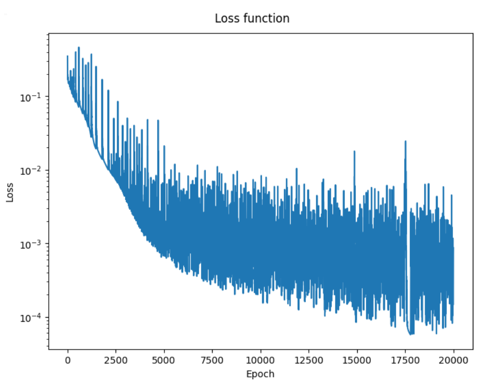
Figure 1: Heat equation. Convergence of the residual loss function.

for plotting the running average of the loss (see Fig. 2),

⬇

average_loss = running_average(initial_loss_values, window=100)

fig, ax = plt.subplots(figsize=(8, 6), dpi=100)

ax.set_title("Initial loss function (running average)")

ax.set_xlabel("Epoch")

ax.set_ylabel("Loss")

ax.plot(average_loss)

ax.set_yscale(’log’)

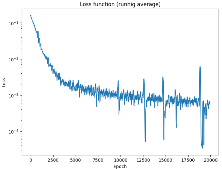
Figure 2: Heat equation. Running average from the convergence of the residual loss function.

for plotting the initial conditions in 2D (see Fig. 3)

⬇

# Plotting

# Initial condition

base_dir = ’.’

x, y, _ = get_initial_points(x_domain, y_domain, t_domain, N_POINTS_PLOT, requires_grad=False)

z = initial_condition(x, y)

fig = plot_color(z, x, y, N_POINTS_PLOT, N_POINTS_PLOT, "Initial condition - exact")

t_value = 0.0

t = torch.full_like(x, t_value)

z = pinn(x, y, t)

fig = plot_color(z, x, y, N_POINTS_PLOT, N_POINTS_PLOT, "Initial condition - PINN")

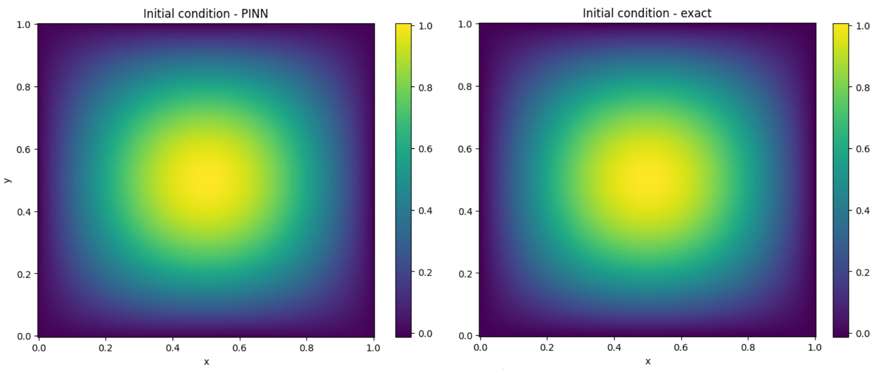
Figure 3: Heat equation. Initial conditions in 2D.

for plotting the initial conditions in 3D (see Fig. 4)

⬇

# Plotting

# Initial condition

x, y, _ = get_initial_points(x_domain, y_domain, t_domain, N_POINTS_PLOT, requires_grad=False)

z = initial_condition(x, y)

fig = plot_3D(z, x, y, N_POINTS_PLOT, N_POINTS_PLOT, "Initial condition - exact")

z = pinn(x, y ,t)

fig = plot_3D(z, x, y, N_POINTS_PLOT, N_POINTS_PLOT, f"Initial condition - pinn")

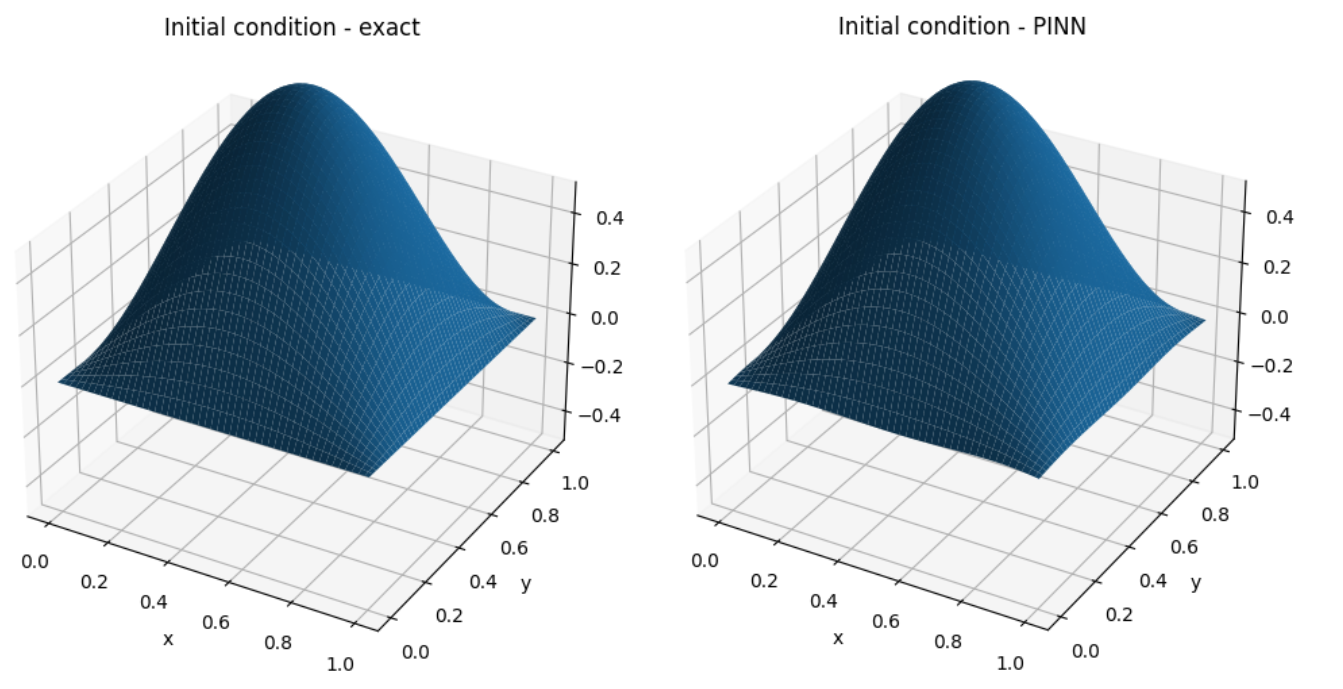
Figure 4: Heat equation. Initial conditions in 3D.

for plotting the snapshots of the solution (see Fig. 5)

⬇

def plot(idx, t_value):

t = torch.full_like(x, t_value)

z = pinn(x, y, t)

fig = plot_color(z, x, y, N_POINTS_PLOT, N_POINTS_PLOT, f"PINN for t = {t_value}")

fig = plot_3D(z, x, y, N_POINTS_PLOT, N_POINTS_PLOT, f"PINN for t = {t_value}")

#plt.savefig(base_dir + ’/img/img_{:03d}.png’.format(idx))

time_values = np.arange(0, TOTAL_TIME, 0.01)

for idx, t_val in enumerate(time_values):

plot(idx, t_value)

z = pinn(x, y, t)

fig = plot_color(z, x, y, N_POINTS_PLOT, N_POINTS_PLOT, f"PINN for t = {t_value}")

fig = plot_3D(z, x, y, N_POINTS_PLOT, N_POINTS_PLOT, f"PINN for t = {t_val}")

#plt.savefig(base_dir + ’/img/img_{:03d}.png’.format(idx))

time_values = np.arange(0, TOTAL_TIME, 0.01)

for idx, t_val in enumerate(time_values):

plot(idx, t_val)

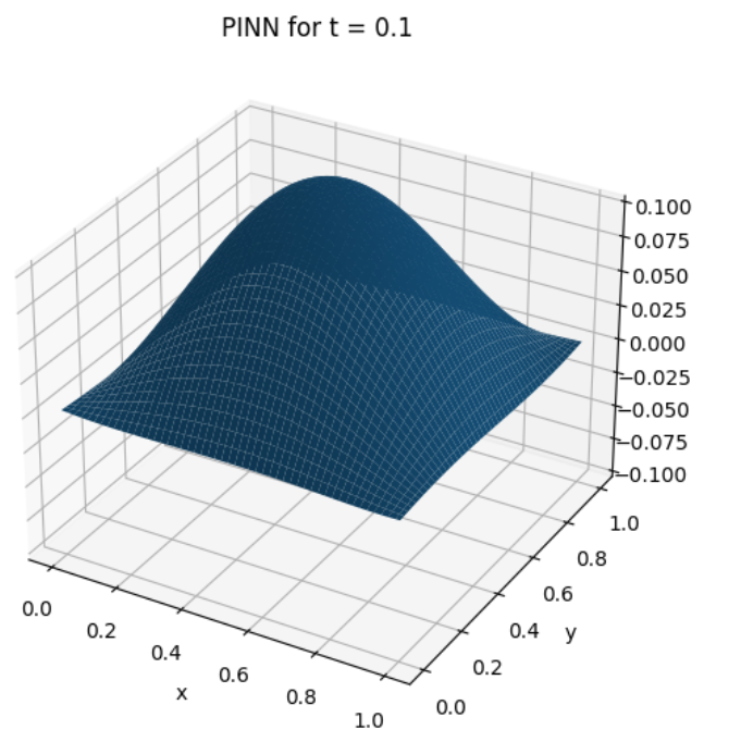
Figure 5: Heat equation. Snapshot from the simulation.

and for the generation of the animated gif with the simulation results.

⬇

from google.colab import drive

drive.mount(’/content/drive’)

import imageio

frames = []

for idx in range(len(time_values)):

image = imageio.v2.imread(base_dir + ’/img/img_{:03d}.png’.format(idx))

frames.append(image)

imageio.mimsave(’./tsunami_wave12.gif’, # output gif

frames, # array of input frames

duration=0.1) # optional: frames per secon

5 Examples of the instantiation

5.1 Heat transfer

In this section, we present the numerical results for the model heat transfer problem described in Section 2. The residual loss function $LOSS_{PDE}(x,y,t)=\left(\frac{\partial PINN(x,y,t)}{\partial t}-\frac{\partial^{2}PINN(x,y,t)}{\partial x^{2}}-\frac{\partial^{2}PINN(x,y,t)}{\partial y^{2}}-f(x,y,t)\right)^{2}$ translates into the following code

⬇

def residual_loss(self, pinn: PINN):

x, y, t = get_interior_points(self.x_domain,

self.y_domain, self.t_domain, self.n_points, pinn.device())

u = f(pinn, x, y, t)

z = self.floor(x, y)

loss = dfdt(pinn, x, y, t, order=1) - \

dfdx(pinn, x, y, t) ** 2 - \

dfdy(pinn, x, y, t) ** 2

We employ the manufactured solution technique, where we assume the solution of the following form

$$u(x,y,t)=\exp^{-2\Pi^{2}t}\sin{\Pi x}\sin{\Pi y}$$ (14)

over $\Omega=[0,1]^{2}$ To obtain this particular solution, we set up the zero Dirichlet boundary conditions, which require the following code

⬇

def boundary_loss_dirichlet(self, pinn: PINN):

down, up, left, right = get_boundary_points(self.x_domain,

self.y_domain, self.t_domain, self.n_points, pinn.device())

x_down, y_down, t_down = down

x_up, y_up, t_up = up

x_left, y_left, t_left = left

x_right, y_right, t_right = right

loss_down = f( pinn, x_down, y_down, t_down )

loss_up = f( pinn, x_up, y_up, t_up )

loss_left = f( pinn, x_left, y_left, t_left )

loss_right = f( pinn, x_right, y_right, t_right )

return loss_down.pow(2).mean() + \

loss_up.pow(2).mean() + \

loss_left.pow(2).mean() + \

loss_right.pow(2).mean()

We also setup the initial state

$$u_{0}(x,y)=\sin{(\Pi x)}\sin{(\Pi y)}$$ (15)

which translates into the following code

⬇

def initial_condition(x: torch.Tensor, y: torch.Tensor) -> torch.Tensor:

res = torch.sin(torch.pi*x) * torch.sin(torch.pi*y)

return res

The default setup of the parameters for this simulation is the following:

⬇

LENGTH = 1.

TOTAL_TIME = 1.

N_POINTS = 15

N_POINTS_PLOT = 150

WEIGHT_RESIDUAL = 1.0

WEIGHT_INITIAL = 1.0

WEIGHT_BOUNDARY = 1.0

LAYERS = 4

NEURONS_PER_LAYER = 80

EPOCHS = 20_000

LEARNING_RATE = 0.002

The convergence of the loss function is presented in Fig. 1. The running average of the loss is presented in Fig. 2. The comparison of exact and trained initial conditions is presented in Fig. 3 in 2D and Fig. 4 in 3D. The snapshot from the simulation is presented in Fig. 5 for time moment $t=0.1$. The mean square error of the computed simulation is presented in Fig. 6. We can see the high accuracy of the trained PINN results.

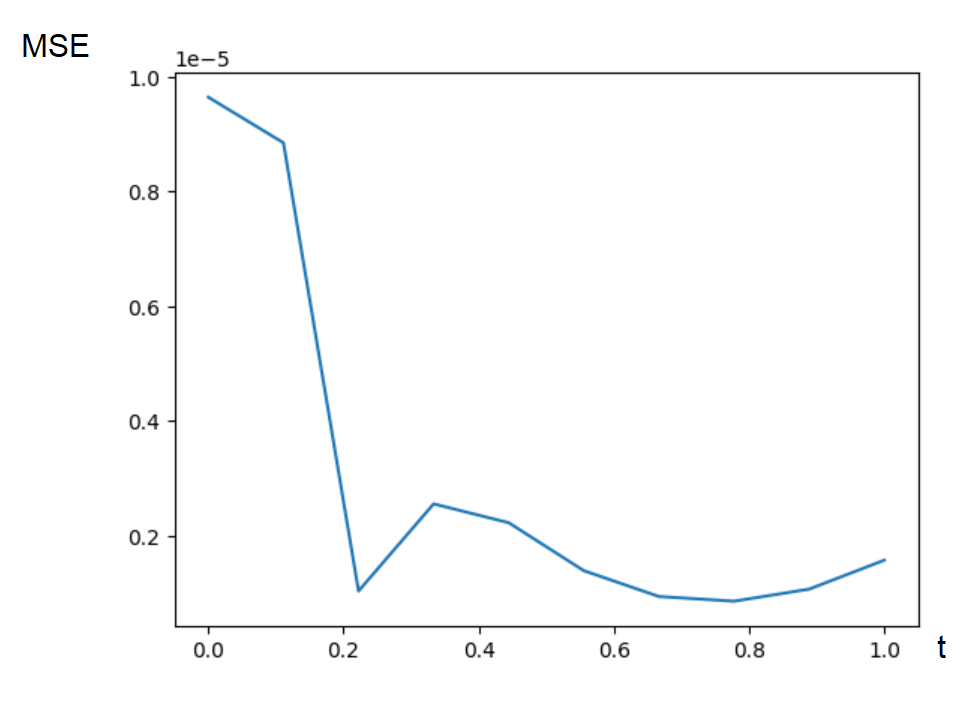
Figure 6: Heat equation. Numerical error of the trained PINN solution to the heat transfer problem with manufactured solution.

5.2 Wave equations

In this section, we consider the simulations of the wave equation, as motivated by the finite element method model described in [8]. Let us consider a strong form of the wave equation: Find $u\in C^{2}(0,1)$ for $(x,y)\in\Omega=[0,1]^{2}$, $t\in[0,T]$ such that

$$\frac{\partial^{2}u(x,y,t)}{\partial t^{2}}-\left(\frac{\partial}{\partial x},\frac{\partial}{\partial y}\right)\cdot\left(g(u(x,y,t)-z(x,y))\left(\frac{\partial u}{\partial x},\frac{\partial u}{\partial y}\right)\right)=0,\quad(x,y,t)\in\Omega\times[0,T],$$ (16)

with initial condition

$$u(x,y,0)=u_{0}(x,y)$$ (17)

and zero-Neumann boundary condition

$$\frac{\partial u}{\partial n}=0\textrm{ }(x,y)\in\partial\Omega$$ (18)

In our simulation, we run the wave propagation in the “swimming pool"; thus, we assume $z(x,y)=0$. It implies some simplifications in the PDE

$$\frac{\partial^{2}u(x,y,t)}{\partial t^{2}}-\left(g\left(\frac{\partial u(x,y,t)}{\partial x}-\cancel{\frac{\partial z(x,y)}{\partial x}}\right)\frac{\partial u(x,y,t)}{\partial x}\right)-\left(g\left(u(x,y,t)-z(x,y)\right)\frac{\partial^{2}u(x,y,t)}{\partial x^{2}}\right)$$

$$-\left(g\left(\frac{\partial u(x,y,t)}{\partial y}-\cancel{\frac{\partial z(x,y)}{\partial y}}\right)\frac{\partial u(x,y,t)}{\partial y}\right)=0-\left(g\left(u(x,y,t)-z(x,y)\right)\frac{\partial^{2}u(x,y,t)}{\partial y^{2}}\right)=0$$ (19)

In the Physics Informed Neural Network approach, the neural network represents the solution,

$$u(x,y,t)=PINN(x,y,t)=A_{n}\sigma\left(A_{n-1}\sigma(...\sigma(A_{1}[x,y,t]+B_{1})...+B_{n-1}\right)+B_{n}$$ (20)

with $A_{i}$ being the matrices representing layers, $B_{i}$ are vectors representing biases, and $\sigma$ is sigmoid activation function [2]. We define the loss function as the residual of the PDE

$$LOSS_{PDE}(x,y,t)=\left(\frac{\partial^{2}PINN(x,y,t)}{\partial t^{2}}-g\left(\frac{\partial PINN(x,y,t)}{\partial x}\right)^{2}-g\left(PINN(x,y,t)-z(x,y)\right)\frac{\partial^{2}PINN(x,y,t)}{\partial x^{2}}\right.$$

$$\left.-g\left(\frac{\partial PINN(x,y,t)}{\partial y}\right)^{2}-g\left(PINN(x,y,t)-z(x,y)\right)\frac{\partial^{2}PINN(x,y,t)}{\partial y^{2}}\right)^{2}$$ (21)

This residual translates into the following code

⬇

def residual_loss(self, pinn: PINN):

x, y, t = get_interior_points(self.x_domain, self.y_domain, self.t_domain,

self.n_points, pinn.device())

u = f(pinn, x, y, t)

z = self.floor(x, y)

loss = dfdt(pinn, x, y, t, order=2) - GRAVITY * ( dfdx(pinn, x, y, t) ** 2

+ (u-z) * dfdx(pinn, x, y, t, order=2) + dfdy(pinn, x, y, t) ** 2

+ (u-z) * dfdy(pinn, x, y, t, order=2)

)

return loss.pow(2).mean()

We also define the loss for training of the initial condition. It is defined as the residual of the initial condition

$$LOSS_{Init}(x,y,0)=\left(PINN(x,y,0)-u_{0}(x,y)\right)^{2}$$ (22)

Similarly, we define the loss of the residual of the boundary conditions

$$LOSS_{BC}(x,y,t)=\left(\frac{\partial PINN(x,y,t)}{\partial n}(x,y,t)-0\right)^{2}$$ (23)

We do not have to change the code for the initial and boundary conditions, we just provide an implementation of the initial state

⬇

def initial_condition(x: torch.Tensor, y: torch.Tensor) -> torch.Tensor:

r = torch.sqrt((x-LENGTH/2)**2 + (y-LENGTH/2)**2)

res = 2 * torch.exp(-(r)**2 * 30) + 2

return res

The convergence of the loss is summarized in Fig. 7. The snapshots of the simulation are presented in Fig. 8.

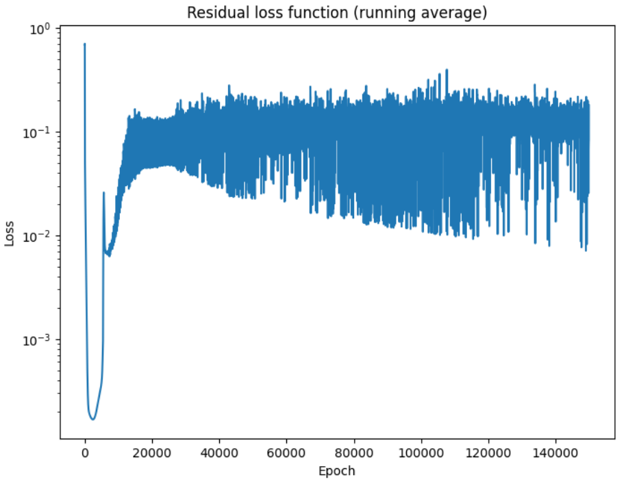
Figure 7: Wave equation. Convergence of the loss function.

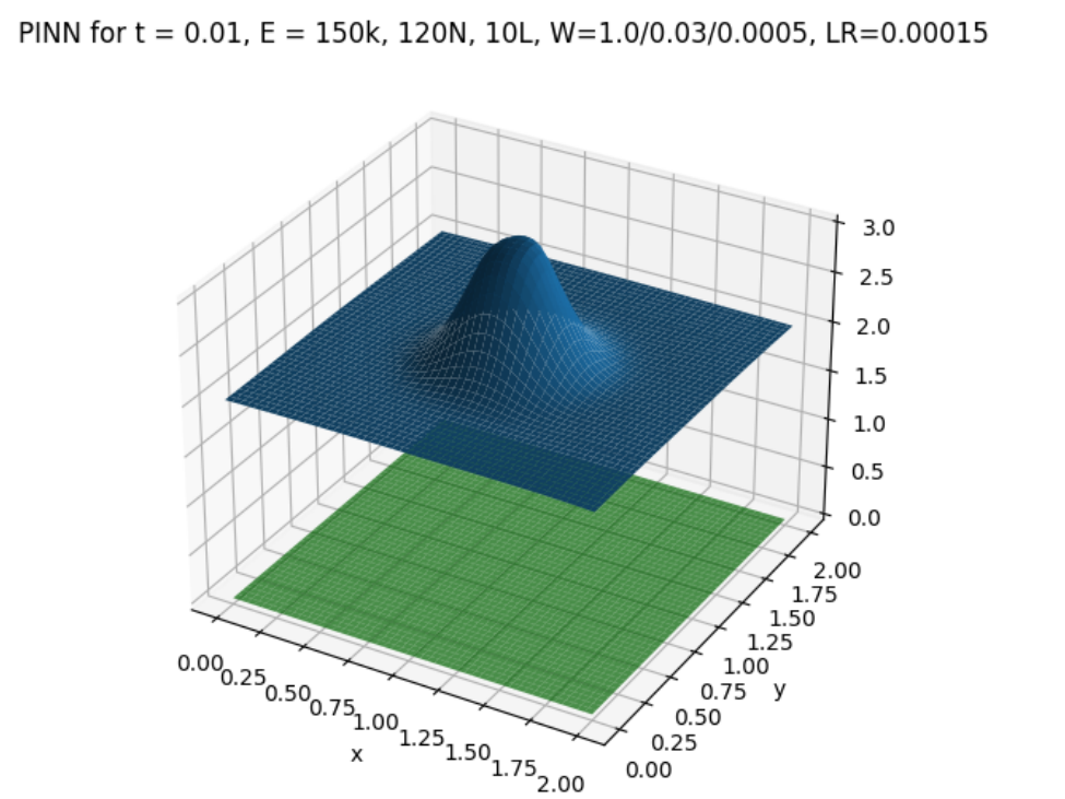
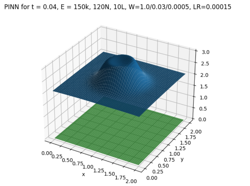
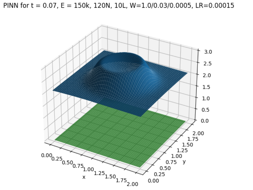
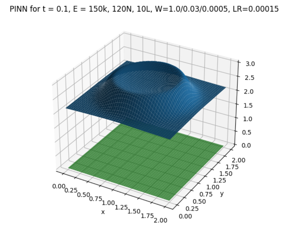
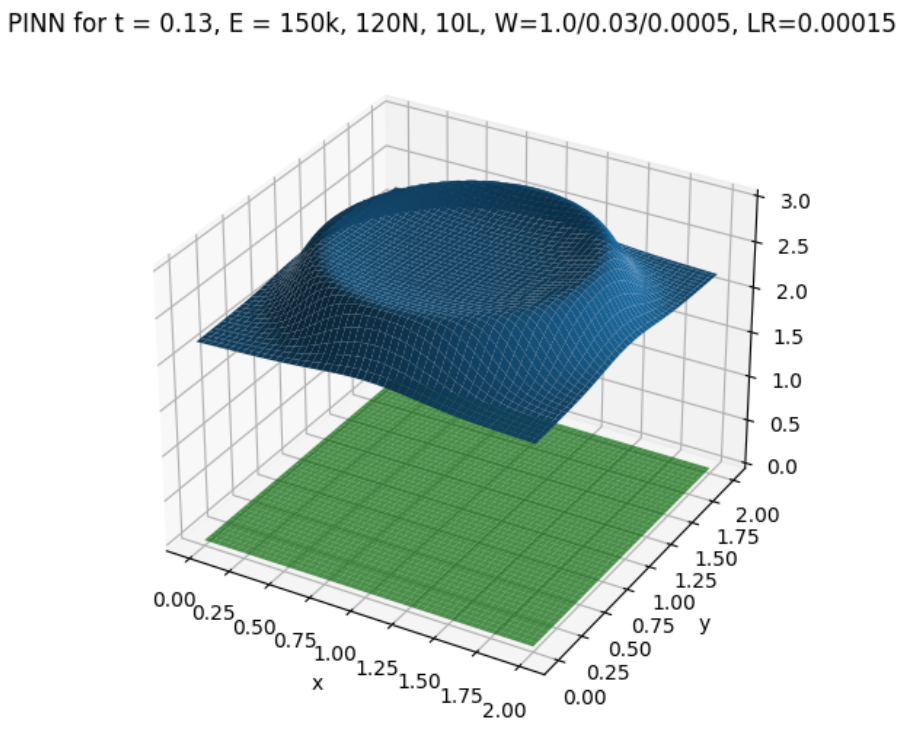
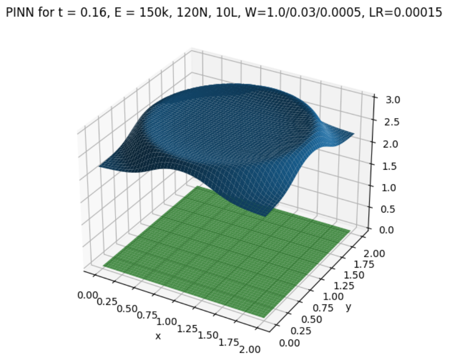
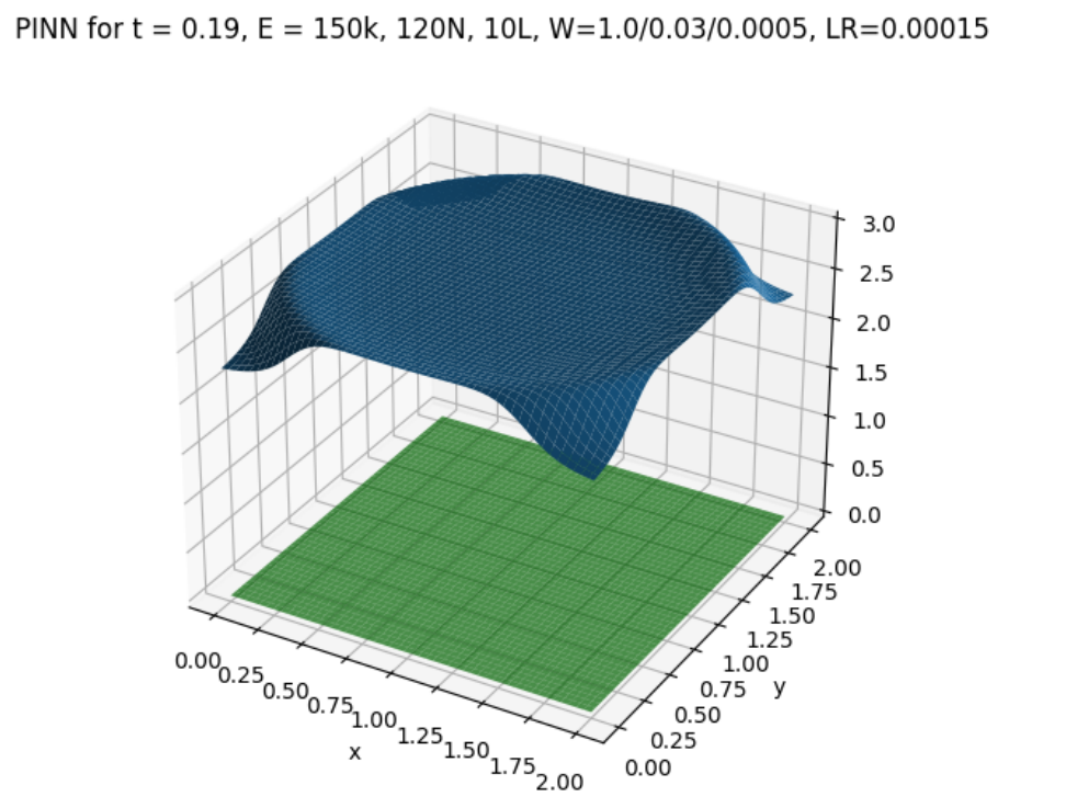
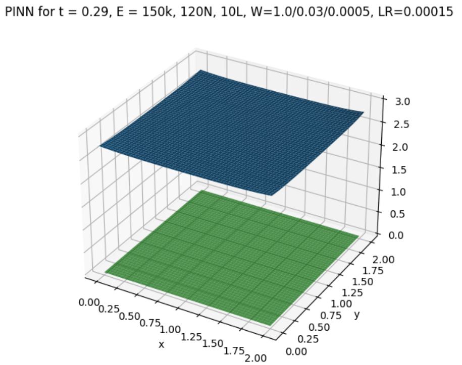
Figure 8: Wave equation simulation.

5.3 Thermal inversion

In this example, we aim to model the thermal inversion effect. The numerical results presented in this section are the PINN version of the thermal inversion simulation performed using isogeometric finite element method code [5] described in [9]. The scalar field $u$ in our simulation represents the water vapor forming a cloud. The source represents the evaporation of the cloud evaporation of water particles near the ground. The thermal inversion effect is obtained by introducing the advection field as the gradient of the temperature. Following [10] we define $\frac{\partial T}{\partial y}=-2$ for lower half of the domain ($y<0.5$), and $\frac{\partial T}{\partial y}=2$ for upper half of the domain ($y>0.5$).

We focus on advection-diffusion equations in the strong form. We seek the cloud vapor concentration field $[0,1]^{2}\times[0,1]\ni(x,y,t)\rightarrow u(x,y,t)\in{\cal R}$

$$\frac{\partial u(x,y,t)}{\partial t}+\left(b(x,y,t)\cdot\nabla\right)u(x,y,t)-\nabla\cdot\left(K\nabla u(x,y,t)\right)=f(x,y,t)\textrm{ }(x,y,t)\in\Omega\times(0,T]$$ (24)

$$\nabla u\cdot n=0\textrm{ in }\partial\Omega\times(0,T]$$ (25)

$$u(x,y,0)=u_{0}(x,y)\textrm{ in }\Omega\times 0$$ (26)

This PDE translates into

$$\frac{\partial u(x,y,t)}{\partial t}+\frac{\partial T(y)}{\partial y}\frac{\partial u(x,y,t)}{\partial y}-0.1\frac{\partial u(x,y,t)}{\partial x^{2}}-0.01\frac{\partial u(x,y,t)}{\partial y^{2}}=f(x,y,t)\textrm{ }(x,y,t)\in\Omega\times(0,T]$$ (28)

$$\nabla u\cdot n=0\textrm{ in }\partial\Omega\times(0,T]$$ (29)

$$u(x,y,0)=u_{0}(x,y)\textrm{ in }\Omega\times 0$$ (30)

In PINN, the neural network represents the solution,

$$u(x,y,t)=PINN(x,y,t)=A_{n}\sigma\left(A_{n-1}\sigma(...\sigma(A_{1}[x,y,t]+B_{1})...+B_{n-1}\right)+B_{n}$$ (32)

where $A_{i}$ are matrices representing DNN layers, $B_{i}$ represent bias vectors, and $\sigma$ is the sigmoid activation function. We define the loss function as the residual of the PDE

$$LOSS_{PDE}(x,y,t)=$$

$$\left(\frac{\partial PINN(x,y,t)}{\partial t}+\frac{\partial T(y)}{\partial y}\frac{\partial PINN(x,y,t)}{\partial y}-0.1\frac{\partial PINN(x,y,t)}{\partial x^{2}}-0.01\frac{\partial PINN(x,y,t)}{\partial y^{2}}-f(x,y,t)\right)^{2}$$ (33)

This residual translates to the following code

⬇

def residual_loss(self, pinn: PINN):

x, y, t = get_interior_points(self.x_domain, self.y_domain, self.t_domain,

self.n_points, pinn.device())

loss = dfdt(pinn, x, y, t).to(device)

- self.dTy(y, t)*dfdy(pinn, x, y, t).to(device)

- self.Kx*dfdx(pinn, x, y, t,order=2).to(device)

- self.Ky*dfdy(pinn, x, y, t, order=2).to(device)

- self.source(y,t).to(device)

return loss.pow(2).mean

We add the definitions of the Kx and Ky variables into the Loss class. We do not change the implementation of the initial and boundary conditions, but we provide the definition of the initial state and forcing

⬇

def source(self,y,t):

d=0.7

res = torch.clamp((torch.cos(t*math.pi) - d)*1/(1-d), min = 0)

res2 = (150 - 1200 * y) * res

res3 = torch.where(t <= 0.3, res2, 0)

res4 = torch.where(y <= 0.125, res3, 0)

return res4.to(device)

During the training, we use the following global parameters

⬇

LENGTH = 1.

TOTAL_TIME = 1.

N_POINTS = 15

N_POINTS_PLOT = 150

WEIGHT_RESIDUAL = 20.0

WEIGHT_INITIAL = 1.0

WEIGHT_BOUNDARY = 10.0

LAYERS = 2

NEURONS_PER_LAYER = 600

EPOCHS = 30_000

LEARNING_RATE = 0.002

The convergence of the loss function is summarized in Fig. 9. The snapshots from the simulations are presented in Fig. 10. In the thermal inversion, the cloud vapor that evaporated from the ground stays close to the ground, due to the distribution of the temperature gradients.

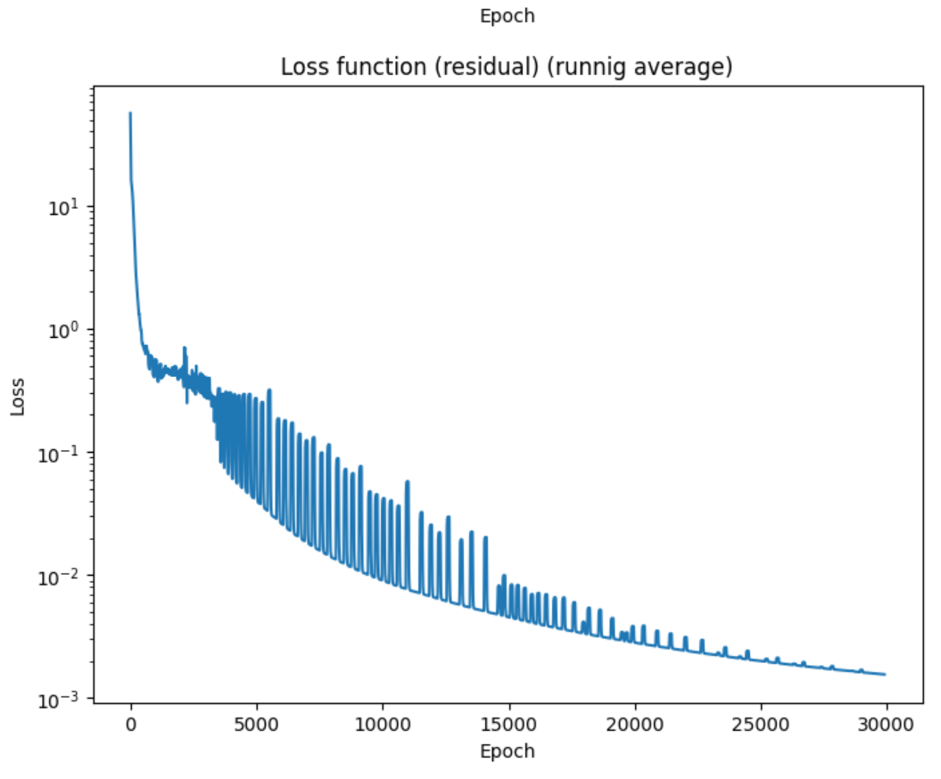
Figure 9: Thermal inversion. Convergence of the loss function.

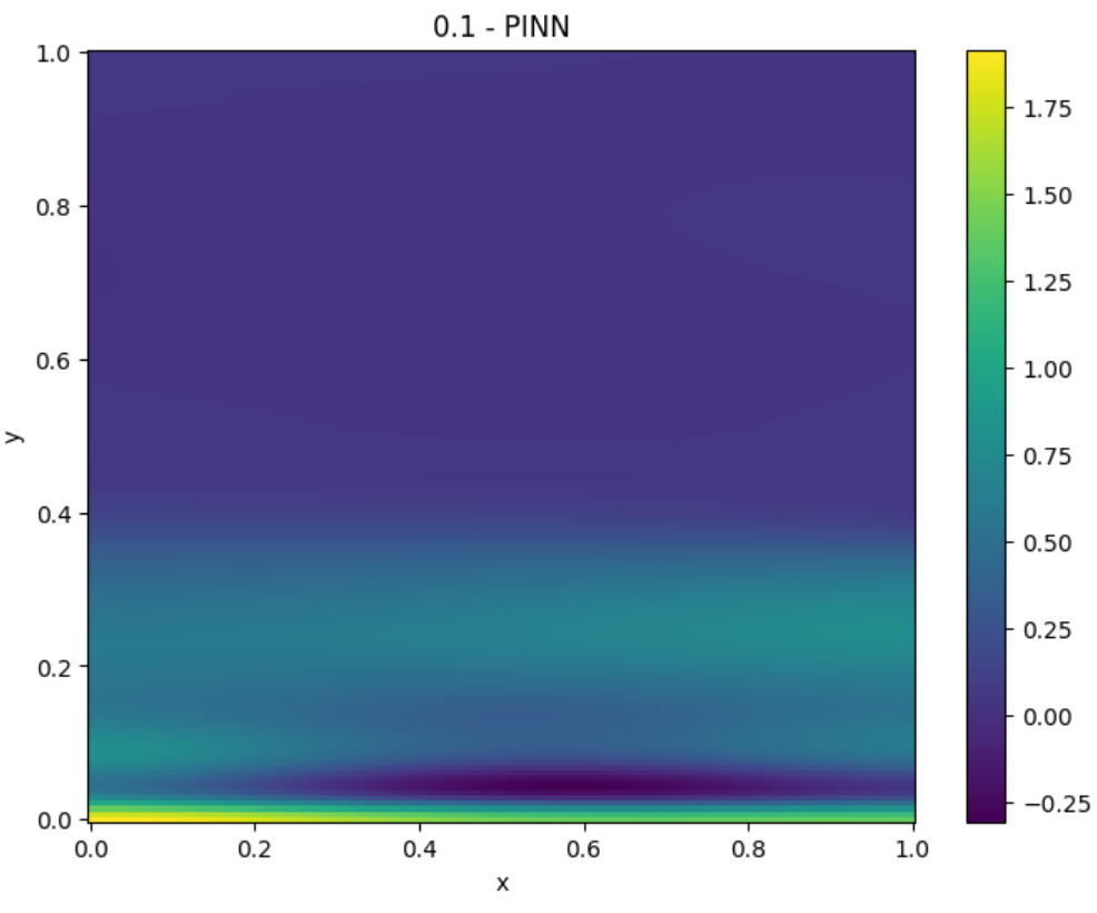
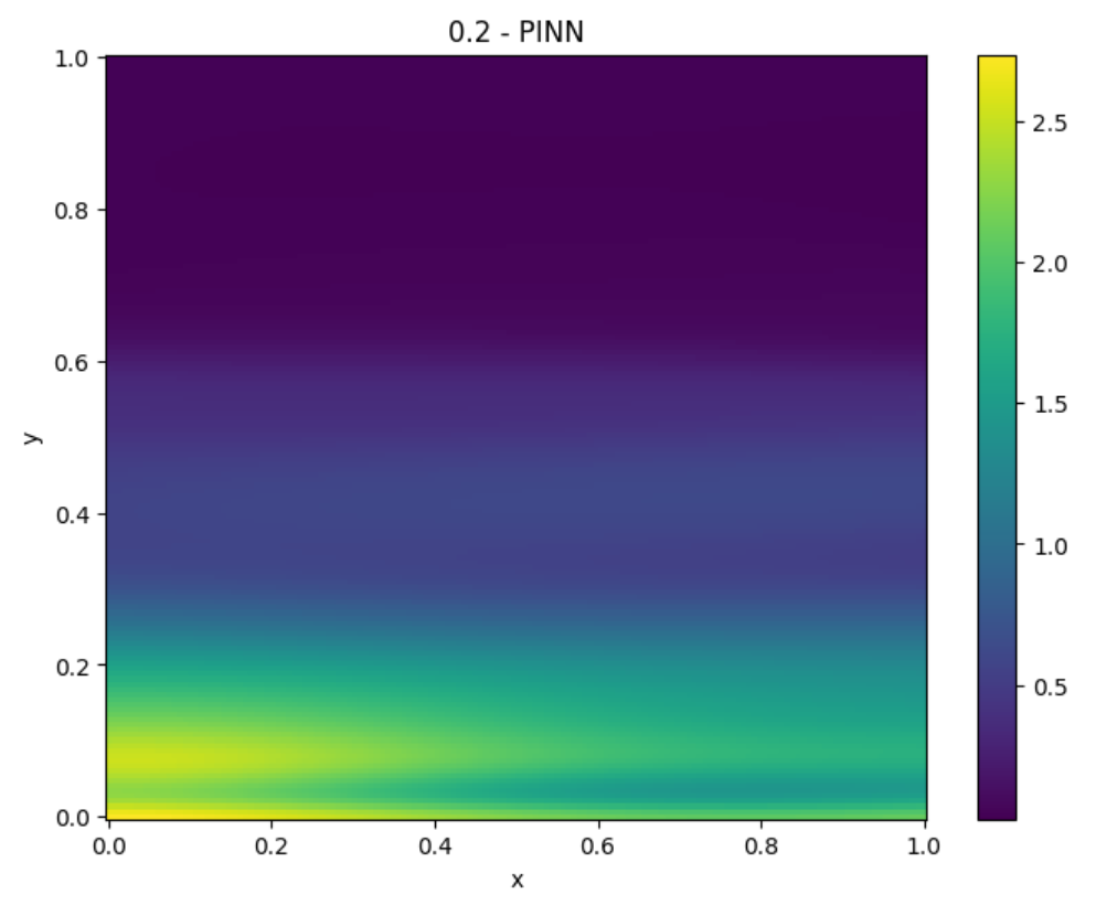
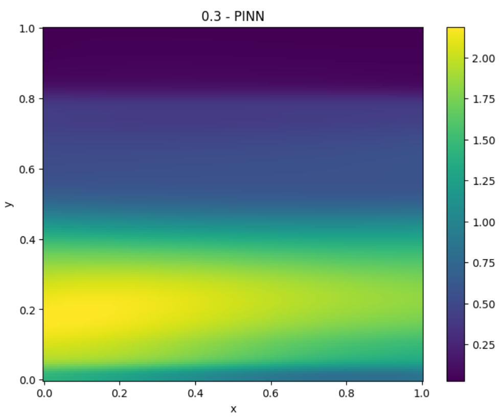
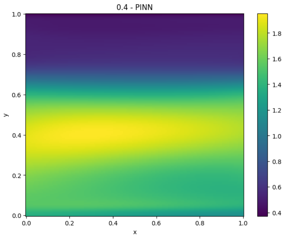
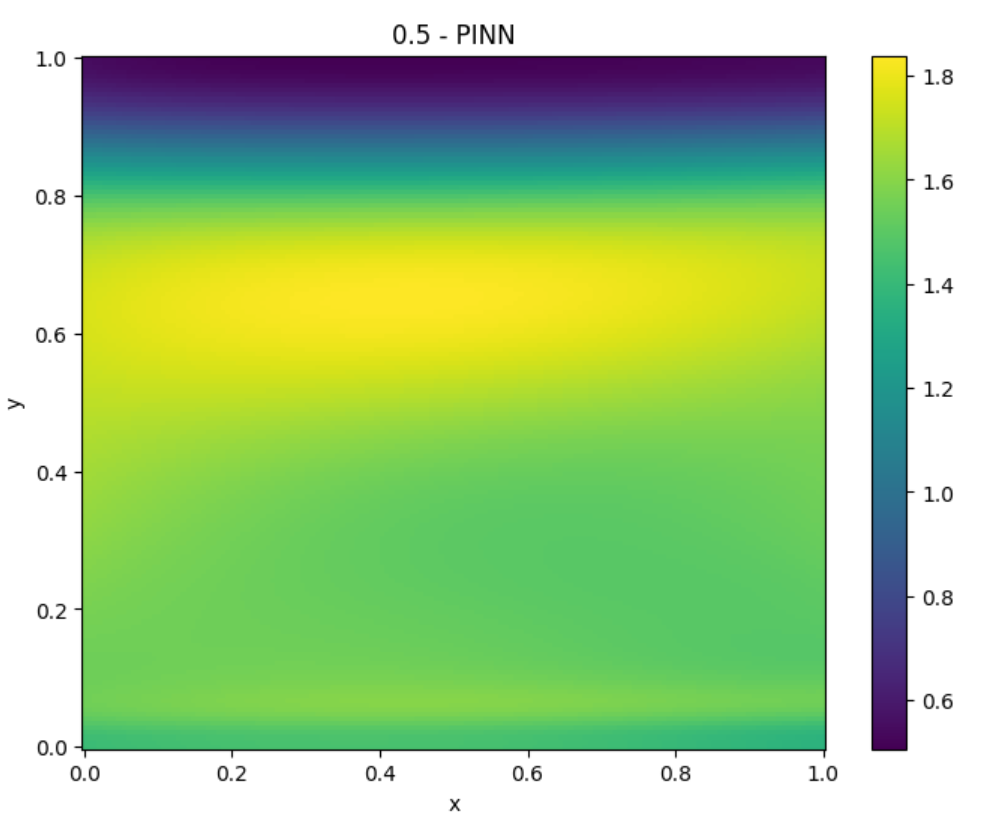
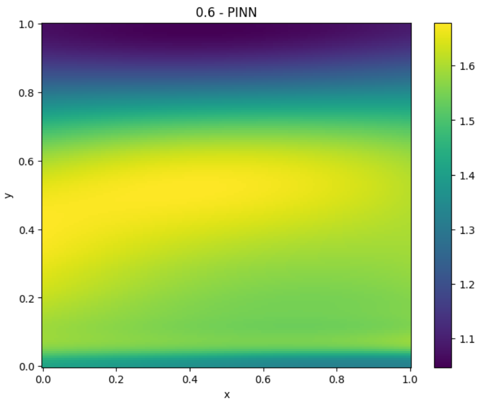
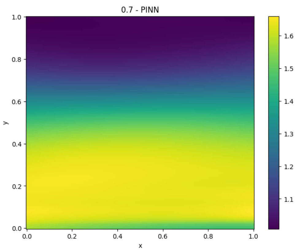
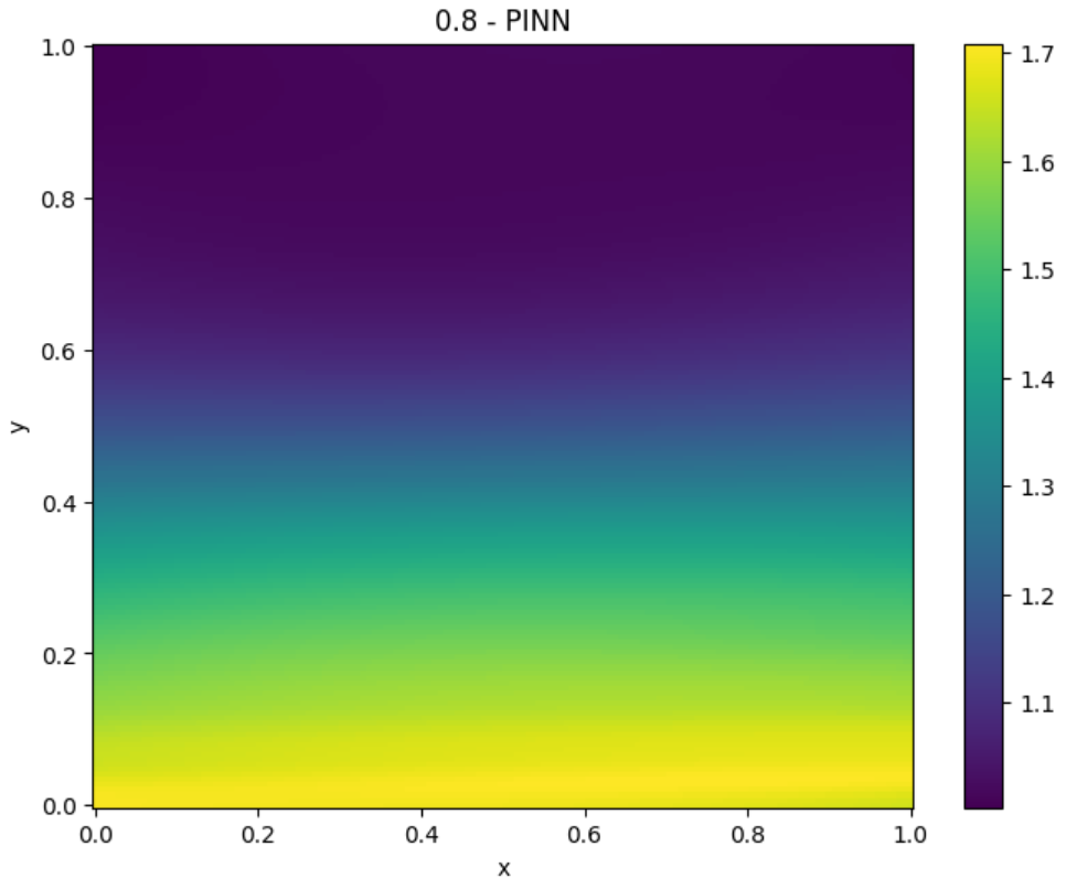
Figure 10: Thermal inversion simulation.

5.4 Tumor growth

The last example concerns the brain tumor growth model, as described in [11]. We seek the tumor cell density $[0,1]^{2}\times[0,1]\ni(x,y,t)\rightarrow u(x,y,t)\in{\cal R}$, such that

$$\frac{\partial u(x,y,t)}{\partial t}=\nabla\cdot\left(D(x,y)\nabla u(x,y,t)\right)+\rho u(x,y,t)\left(1-u(x,y,t)\right)\textrm{ }(x,y,t)\in\Omega\times(0,T]$$ (34)

$$\nabla u\cdot n=0\textrm{ in }\partial\Omega\times(0,T]$$ (35)

$$u(x,y,0)=u_{0}(x,y)\textrm{ in }\Omega\times 0$$ (36)

which translates into

$$\frac{\partial u(x,y,t)}{\partial t}-\frac{\partial D(x,y)}{\partial x}\frac{\partial u(x,y,t)}{\partial x}-D(x,y)\frac{\partial^{2}u(x,y,t)}{\partial x^{2}}$$

$$-\frac{\partial D(x,y)}{\partial y}\frac{\partial u(x,y,t)}{\partial y}-D(x,y)\frac{\partial^{2}u(x,y,t)}{\partial x^{y}}-\rho u(x,y,t)\left(1-u(x,y,t)\right)=0$$ (38)

Here, $D(x,y)$ represents the tissue density coefficient, where $D(x,y)=0.13$ for the white matter, $D(x,y)=.013$ for the gray matter, and $D(x,y)=0$ for the cerebrospinal fluid (see [11] for more details). Additionally, $\rho=0.025$ denotes the proliferation rate of the tumor cells. We simplify the model, and remove the derivatives of the tissue density coefficient:

$$\frac{\partial u(x,y,t)}{\partial t}-D(x,y)\frac{\partial^{2}u(x,y,t)}{\partial x^{2}}-D(x,y)\frac{\partial^{2}u(x,y,t)}{\partial x^{y}}-\rho u(x,y,t)\left(1-u(x,y,t)\right)=0.$$ (39)

As usual, in PINN, the neural network represents the solution,

$$u(x,y,t)=PINN(x,y,t)=A_{n}\sigma\left(A_{n-1}\sigma(...\sigma(A_{1}[x,y,t]+B_{1})...+B_{n-1}\right)+B_{n}$$ (40)

with $A_{i}$, and $B_{i}$ representing matrices and bias vectors, and $\sigma$ is the sigmoid activation function. We define the loss function as the residual of the PDE

$$LOSS_{PDE}(x,y,t)=$$

$$\left(\frac{\partial u(x,y,t)}{\partial t}-\frac{\partial D(x,y)}{\partial x}\frac{\partial u(x,y,t)}{\partial x}-D(x,y)\frac{\partial^{2}u(x,y,t)}{\partial x^{2}}\right.$$

$$\left.-\frac{\partial D(x,y)}{\partial y}\frac{\partial u(x,y,t)}{\partial y}-D(x,y)\frac{\partial^{2}u(x,y,t)}{\partial x^{y}}-\rho u(x,y,t)\left(1-u(x,y,t)\right)\right)^{2}$$ (41)

This translates into the following code:

⬇

def residual_loss(self, pinn: PINN):

x, y, t = get_interior_points(

self.x_domain, self.y_domain,

self.t_domain, self.n_points,

pinn.device())

rho = 0.025

def D_fun(x, y) -> torch.Tensor:

res = torch.zeros(x.shape, dtype=x.dtype, device=pinn.device())

dist = (x-0.5)**2 + (y-0.5)**2

res[dist < 0.25] = 0.13

res[dist < 0.02] = 0.013

return res

D = D_fun(x, y)

u = f(pinn, x, y, t)

loss = dfdt(pinn, x, y, t) \

- D * dfdx(pinn, x, y, t, order=2) \

- D * dfdy(pinn, x, y, t, order=2) \

- rho * u * (1 - u)

return loss.pow(2).mean()

The initial and boundary condition loss functions are unchanged. The initial state is given as follows:

⬇

def initial_condition(x: torch.Tensor, y: torch.Tensor) -> torch.Tensor:

d = torch.sqrt((x-0.6)**2 + (y-0.6)**2)

res = -d**2 - 4*d + 0.4

res = res * (res > 0)

return res

We setup the following model parameters

⬇

LENGTH = 1.

TOTAL_TIME = 1.

N_POINTS = 20

N_POINTS_PLOT = 150

WEIGHT_RESIDUAL = 1.0

WEIGHT_INITIAL = 1.0

WEIGHT_BOUNDARY = 1.0

LAYERS = 4

NEURONS_PER_LAYER = 80

EPOCHS = 50_000

LEARNING_RATE = 0.005

We summarize in Fig. 11 the convergence of the loss function. We also show how the initial data has been trained in Fig. 12. Additionally, Fig. 13 presents the snapshots from the simulation.

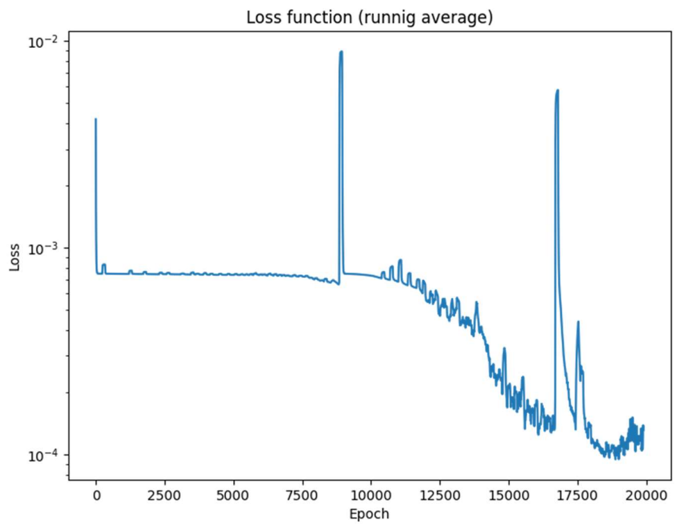
Figure 11: Tumor growth. Convergence of the loss function.

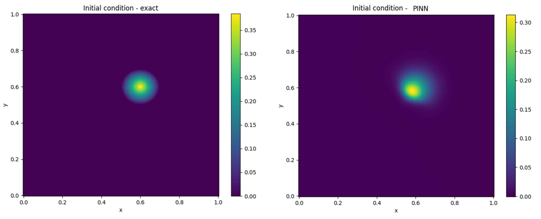
Figure 12: Tumor growth. Convergence of the loss function.

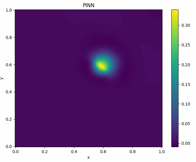
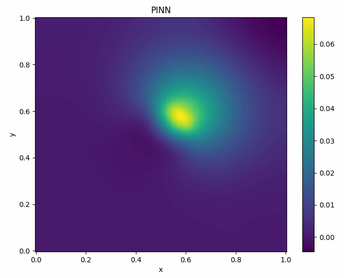
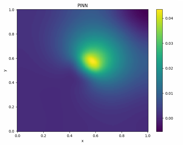
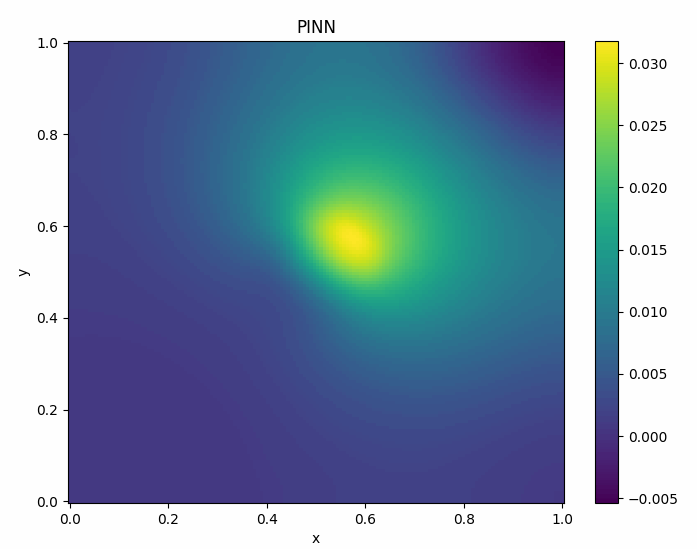
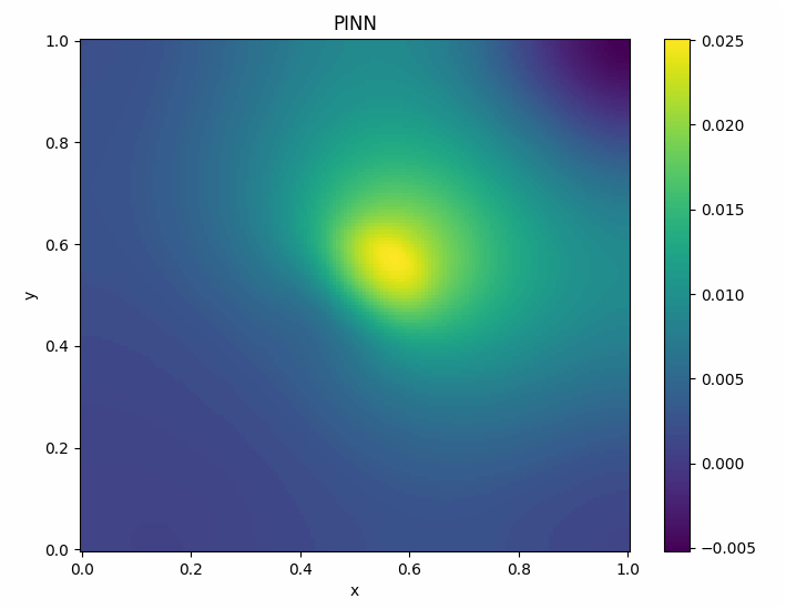
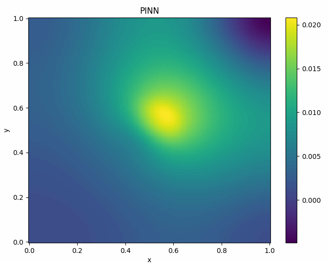
Figure 13: Tumor growth. Snapshots from the simulation.

6 Conclusions

We have created a code https://github.com/pmaczuga/pinn-notebooks that can be downloaded and opened in the Google Colab. It can be automatically executed using Colab functionality. The code provides a simple interface for running two-dimensional time-dependent simulations on a rectangular grid. It provides an interface to define residual loss, initial condition loss, and boundary condition loss. It provides examples of Dirichlet and Neumann boundary conditions. The code also provides routines for plotting the convergence, generating snapshots of the simulations, verifying the initial condition, and generating the animated gifs. We also provide four examples, the heat transfer, the wave equation, the thermal inversion from advection-diffusion equations, and the brain tumor model.

7 Acknowledgements

The work of Maciej Paszyński, Witold Dzwinel, Paweł Maczuga, and Marcin Łoś was supported by the program “Excellence initiative - research university" for the AGH University of Science and Technology. The visit of Maciej Paszyński at Oden Institute was partially supported by J. T. Oden Research Faculty Fellowship.

References

- [1] M. Raissi, P.Perdikaris, G.E.Karniadakis, Physics-informed neural networks: A deep learning framework for solving forward and inverse problems involving nonlinear partial differential equations, Journal of Computational Physics, 378 (2019) 686-707
- [2] Paweł Maczuga, Maciej Paszyński, Influence of Activation Functions on the Convergence of Physics-Informed Neural Networks for 1D Wave Equation, Computational Science – ICCS 2023: 23rd International Conference, Prague, Czech Republic, July 3-5, 2023, Proceedings, Part I, (2023) 74–88, https://doi.org/10.1007/978-3-031-35995-8_6
- [3] D. P. Kingma, J. Lei Ba, ADAM: A method for stochastic optimization, arXiv:1412.6980 (2014)
- [4] Yang Chen, Yongfu Xu, Lei Wang, Tianyi Li, Modeling water flow in unsaturated soils through physics-informed neural network with principled loss function, Computers and Geotechnics, 161 (2023) 105546, https://doi.org/10.1016/j.compgeo.2023.105546
- [5] Marcin Łoś, Maciej Woźniak, Maciej Paszyński, Andrew Lenharth, Keshav Pingali, IGA-ADS : Isogeometric Analysis FEM using ADS solver, Computer & Physics Communications, 217 (2017) 99-116.
- [6] Marcin Łoś, Maciej Paszyński, Adriank Kłusek, Witold Dzwinel, Application of fast isogeometric L2 projection solver for tumor growth simulations, Computer Methods in Applied Mechanics and Engineering, 316 (2017) 1257-1269.
- [7] Marcin łoś, Adriank Kłusek, M. Amber Hassaan, Keshav Pingali, Witold Dzwinel, Maciej Paszyński. Parallel fast isogeometric L2 projection solver with GALOIS system for 3D tumor growth simulations, Computer Methods in Applied Mechanics and Engineering, 343 (2019) 1-22.
- [8] Paweł Maczuga, Albert Oliver-Serra, Anna Paszyńska, Eirik Valseth, Maciej Paszyński, Graph-grammar based algorithm for asteroid tsunami simulations, Journal of Computational Science, 64 (2022) 101856, https://doi.org/10.1016/j.jocs.2022.101856.
- [9] Krzysztof Misan, Weronika Ormaniec, Adam Kania, Maciej Kozieja, Marcin łoś, Dominik Gryboś, Jaciek Leszczyński, Maciej Paszyński, Fast isogeometric analysis simulationsof a process of air pollution removal byartificially generated shock waves, Computational Science – ICCS 2022: 22rd International Conference, London, UK, June 21-23, 2022, Proceedings, Part I, (2022) 298-311, https://link.springer.com/chapter/10.1007/978-3-031-08757-8_26
- [10] U.S. Standard Atmosphere vs. Altitude, Engineering ToolBox (2003) https://www.engineeringtoolbox.com/standard-atmosphere-d_604.html,
- [11] Andy Zhu, Jonathan Vo, John Lowengrub, Accelerating Parameter Inference in Diffusion-Reaction Models of Glioblastoma Using Physics-Informed Neural Networks https://www.siam.org/Portals/0/Publications/SIURO/Vol15/S147281R.pdf?ver=2022-10-11-122057-963
- [12] Lu Lu, Xuhui Meng, Zhiping Mao, George Em Karniadakis, DeepXDE: A deep learning library for solving differential equations, SIAM Review, 63(1), (2021) 208-228.
- [13] Wei Peng and Jun Zhang and Weien Zhou and Xiaoyu Zhao and Wen Yao and Xiaoqian Chen, IDRLnet: A Physics-Informed Neural Network Library, arxiv.2107.04320 (2021)
- [14] Somdatta Goswami, Cosmin Anitescu, Souvik Chakraborty, Timon Rabczuk, Transfer learning enhanced physics informed neural network for phase-field modeling of fracture, Theoretical and Applied Fracture Mechanics, 106 (2020) 102447, 10.1016/j.tafmec.2019.102447
- [15] Ehsan Haghighat, Maziar Raissi, Adrian Moure, Hector Gomez, Ruben Juanes, A physics-informed deep learning framework for inversion and surrogate modeling in solid mechanics, Computer Methods in Applied Mechanics and Engineering, 379 (2021) 1879-2138, 10.1016/j.cma.2021.113741