ECGNet: A generative adversarial network (GAN) approach to the synthesis of 12-lead ECG signals from single lead inputs

Abstract

Electrocardiography (ECG) signal generation has been heavily explored using generative adversarial networks (GAN) because the implementation of 12-lead ECGs is not always feasible. The GAN models have achieved remarkable results in reproducing ECG signals but are only designed for multiple lead inputs and the features the GAN model preserves have not been identified—limiting the generated signals use in cardiovascular disease (CVD)-predictive models. This paper presents ECGNet which is a procedure that generates a complete set of 12-lead ECG signals from any single lead input using a GAN framework with a bidirectional long short-term memory (LSTM) generator and a convolutional neural network (CNN) discriminator. Cross and auto-correlation analysis performed on the generated signals identifies features conserved during the signal generation—i.e., features that can characterize the unique-nature of each signal and thus likely indicators of CVD. Finally, by using ECG signals annotated with the CVD-indicative features detailed by the correlation analysis as inputs for a CVD-onset-predictive CNN model, we overcome challenges preventing the prediction of multiple-CVD targets. Our models are experimented on 15s 12-lead ECG dataset recorded using MyoVista’s wavECG. Functional outcome data for each patient is recorded and used in the CVD-predictive model. Our best GAN model achieves state-of-the-art accuracy with Fréchet Distance (FD) scores of 4.73, 4.89, 5.18, 4.77, 4.71, and 5.55 on the V1-V6 pre-cordial leads respectively and shows strength in preserving the P-Q segments and R-peaks in the generated signals. To the best of our knowledge, ECGNet is the first to predict all of the remaining eleven leads from the input of any single lead. Because of ECGNet’s ability to conserve aspects of the PQRST complex, our work is useful for feature extraction that combats the black box nature of the GAN signal generation and ultimately future CVD-predictive models.

ECGNet: A generative adversarial network (GAN) approach to the synthesis of 12-lead ECG signals from single lead inputs

Max Bagga Department of Computer Science Emory University Atlanta, GA, 30322, USA max.bagga@emory.edu                        Hyunbae Jeon Department of Computer Science Emory University Atlanta, GA, 30322, USA harry.jeon@emory.edu                        Alex Issokson Department of Computer Science Emory University Atlanta, GA, 30322, USA alex.issokson@emory.edu

1 Introduction

With cardiovascular disease (CVD) being the leading cause of death, understanding CVD predictors is vital Roth et al. (2020). Traditionally, cardiologists can use twelve-lead electrocardiography (ECG) signals to predict major CVD events near onset through the diagnosis of risk factors Dawber et al. (1952). These risk factors are determined by observing abnormal electrical signal patterns produced by each lead in the ECG Chiou et al. (2021). However, these patterns tend to become recognizable to cardiologists only near inevitable CVD onset Ebrahimi et al. (2020). Consequently, through the availability of large data sets of patients’ ECG signals, there has been a growing interest to use deep learning (DL) algorithms to extract features of ECG signals and use them to predict CVD before irreversible onset Li and Boulanger (2020). Despite the advancement in constructing DL-based CVD-predictive models, clinical implementation is challenging because of the models’ inability to classify multiple-disease targets Stracina et al. (2022).
CVD manifests into disorders that can be categorized: structural heart disease, functional heart disease, and hemodynamic disorders. Several studies have proposed DL models to overcome the multiple-disease target barrier by predicting CVDs within a single category. The convolutional neural network (CNN) rECHOmmend combines the outcomes of multiple structural diseases into a single prediction that outperforms single-disease target models Ulloa-Cerna et al. (2022). While rECHOmmend takes the indicators of multiple different structural CVDs and successfully predicts future onset of generic structural CVD, it fails to classify the onset of a specific structural CVD. Moreover, deep learning models predicting functional heart disease do not significantly outperform classical risk calculators, and those that are on par are single-disease target models—i.e. the models make predictions on just one functional heart disease Zhou et al. (2021). Therefore, clinical implementation is still limited by the inability to specifically classify a disease or take multiple disease features as inputs Stracina et al. (2022). Zhou et al. (2021) argued that deep learning models could add unnecessary complexity and make it hard to investigate crucial feature inputs due to their black box nature. Applying this logic from Zhou et al. (2021), because the true interactions between the input variables of rECHOmmend are obscured by the CNN’s black box, the process cannot be extended to solve the functional heart disease models’ inabilities to take multiple disease inputs and vice versa.
In this paper, we present ECGNet: a Generative Adversarial Network (GAN) model with a bidirectional grid long short-term memory (LSTM) generator and a CNN discriminator trained to be able to reconstruct a complete twelve-lead ECG lead signal set from an input of any one ECG lead signal. The latent features conserved by the GAN model will be extracted from the reconstructed signals using signal cross-correlation and passed as input to another CNN model to predict the onset of multiple structural, functional, and hemodynamic CVDs. We hypothesize that our method can successfully classify multiple-disease targets because by first reconstructing ECG signals and identifying the conserved electrical motifs, we can understand the distinguishing ECG characteristics that the model actually uses, and thus the black-box process previously preventing transfer learning can be illuminated. Our approach uses a bidirectional LSTM-CNN GAN because one LSTM dimension can encode the signal’s temporal trends while the other can encode the other features Hazra and Byun (2020). Zhu et al. (2019) used a bidirectional LSTM-CNN GAN model to generate entire 12-signal data sets from patient features—a similar outcome as ours but with features instead of signals as inputs.
Our approach is evaluated on ECG and functional outcome data from 976 patients with diverse racial, gender, physical, socioeconomic, and medical histories (Section 4). The models operate on the 15-second MyoVista wavECG recordings Sengupta et al. (2018a, b) and over 2000 functional outcomes—e.g., biometrics and disease diagnosis—collected for each patient. We expect our experiments to show that our GAN architecture can recreate a full set of ECG signals from any single ECG lead input that the CNN discriminator cannot consistently distinguish from the actual signals. The signal cross-correlation analysis is expected to identify electric motifs that are conserved in intra-individual ECG signals. With the predictive model taking the conserved electric motifs as inputs, the onsets of CVDs are expected to be predicted and classified.
This work makes three main contributions as follows:

1. We train a GAN model to reconstruct the remaining eleven ECG lead signals from an input of any single ECG leads

2. We extract connections between each reconstructed signal’s characteristics

3. The extracted features are used as inputs to predict and classify multiple CVDs

To the best of our knowledge, this is the first work that reconstructs all twelve ECG signals from the input of any one lead signal.

2 Related Work

The ECGNet procedure focuses on three aspects: reconstructing electrocardiography (ECG) lead signals, mathematical feature extraction from ECG lead signals, and deep learning methods for predicting cardiovascular disease (CVD).

2.1 Reconstructing ECG Lead Signals

The task of reconstructing ECG lead signals is not a new endeavor. Toyoshima et al. (1958) attempted to reconstruct the QRS ECG complexes by summing the ventricular activation or electrical potential changes of the heart in order to diagnose myocardial infarction; however, as demonstrated by Oosterom (2002), the accurate diagnosis of CVD by these methods cannot proceed without prior knowledge of the QRS complex trends corresponding to the CVD and performing the inverse operation on the ECG signal to identify the electrical potential changes of the heart. The mechanism proposed by Toyoshima et al. (1958) is thus rendered obsolete as the QRS trends are what the mechanism attempts to establish yet is also required to make the mechanism accurate. This circular challenge persists throughout modern techniques as well and subsequently is a problem we attempt to circumnavigate by first using the GAN model (3.2) to identify the latent motifs of ECG signal leads (5) and then using the motifs as inputs to the predictive model (3.4).
Drew et al. (2002) was the first to construct multiple lead signals from the input of other lead signals. Using mathematical interpolation on a reduced lead data set, the four missing precordial lead signals were reconstructed in order to diagnose arrhythmia and myocardial ischemia. The reconstructed lead signals preserved the features of the CVDs. Consequently, if the interpolation is clinically implemented, the eight leads can be placed optimally instead of in their traditional twelve-lead placement. Despite the great work of Drew et al. (2002), the interpolation cannot be generalized to even a particular category of CVDs as the eliminated leads of the analysis are invaluable in the diagnosis of other CVDs; therefore, with the advent of DL, many studies have sought to reconstruct ECG lead signals without losing the features of the eliminated leads.
A major breakthrough was made when Sohn et al. (2020) used a LSTM Network to reconstruct a full twelve-lead ECG set from the signal inputs of a portable three-lead ECG hardware. The network outperformed a three-lead input interpolation approach proposed by Hsu and Wu (2014) which already had state-of-the-art results proving the viability of long-term, reduced-lead ECG portable monitoring. This analysis, in addition to a single-electrode device proposed by Lee et al. (2017a), validates the feasibility and clinical viability of our full-set derivation from just two leads. Further analyses verify the necessity of DL in the reconstruction of ECG lead signals either by comparing DL performance to the previous interpolation approaches Grande-Fidalgo et al. (2021); Craven et al. (2017) or by highlighting avenues facilitated only by the DL approach Lee et al. (2017a). Although these DL models accomplish their intended goals, they fail to classify multiple-disease targets much like the aforementioned structural CVD predictor rECHOmmend Ulloa-Cerna et al. (2022) and functional CVD models Zhou et al. (2021). Our approach aims to overcome the shortcomings of these models by using the conserved signal patterns identified by the GAN model to predict multiple-disease targets. Seo et al. (2022) attempted to reconstruct a full twelve-lead ECG from the slightly more ambitious one-lead input by also using a GAN model; however, their study is limited to reconstruction solely considering the limb lead I as the input and does not aim to classify CVD motifs in the reconstructed signals. Therefore, our work is distinguished because our model will take any single lead’s signal to not only reconstruct the remaining signals but to identify highly conserved signal patterns and use the motifs to predict CVD onset: a more informative task.
The methods of our approach can be divided into two categories: pre-processing (3.1) and model design (3.2, 5, 3.4). There has been a concerted effort to use DL to denoise ECG signals Mir and Singh (2021); Singh and Pradhan (2021) and to classify the various components of the heartbeat Burguera (2019); He et al. (2018)—both of which are used as inputs for our GAN model. While these efforts have fruitful results, implementing these models in our pre-processing efforts may introduce training bias (or they may not be substantially cross-validated to be compatible with our dataset) which will be exasperated in the downstream components of our approach; therefore, we adapted a purely mathematical Daubechie wavelet denoising and a non-DL-based heartbeat classification pre-processing procedure validated by Hazra and Byun (2020) and Kachuee et al. (2018) respectively.
Zhu et al. (2019) was the first to show that Electrocardiogram (ECG) signals can be generated using a generative adversarial network (GAN) model where a bidirectional long short-term memory (LSTM) framework is used as a generator while a convolutional neural network (CNN) is used as the discriminator. The model was successfully used to synthesize complete 12-signal data sets from patient features. Given the great success of this framework, we believe that adapting it to take signal inputs instead of patient features can improve the quality of the signal generated allowing for effective classification. Hazra and Byun (2020) used the same model architecture as Zhu et al. (2019) and significantly improved the resolution of the signals generated by tuning the pre-processing and updating both the convolutional and pooling layers of the CNN discriminator. The GAN model’s resulting signals will subsequently be classified (5)—aided by this improved reconstructed signal resolution—providing further support for the architecture. The 15s twelve-lead ECG data used by our analysis is also the input format used in both the adapted pre-processing methods Hazra and Byun (2020); Kachuee et al. (2018) and the various architectures Zhu et al. (2019); Hazra and Byun (2020).

2.2 Mathematical Feature Extraction

Ramli and Ahmad (2003) proved that by taking the cross-correlation between any two signals and by comparing the auto-correlation function of the signals to the original signal, the dependent features can be extracted. Attempts to verify this process have produced successful models identifying specific arrhythmia-indicating signal features Chiu et al. (2005) and even drowsiness predictors Lee et al. (2017b). The analysis of Ramli and Ahmad (2003) was performed between leads from the same person; therefore, the novelty of our approach does not derive from the use of this technique, but because it is used to unveil the properties of the lead signals that the GAN model preserves. By piercing the black box this way, transfer learning can occur—i.e., applying the learning of ECG signal synthesis to the prediction of CVD.

2.3 Deep Learning Methods for Predicting Cardiovascular Disease

CNN models have been remarkably successful using annotated ECG signal inputs to predict CVD of a signal type Wu et al. (2021); Shankar et al. (2020); Dutta et al. (2020). Sajja and Kalluri (2020) validated the superiority of CNN models in this regard by comparing their performance to that of various other machine-learning algorithms. Furthermore, attempts to involve CNN models in CVD-predictive transfer learning have had preliminary successes and thus they can be the vehicle of multiple-disease prediction Weimann and Conrad (2021). Considering this, a predictive CNN model taking the conserved signal motifs identified in the signal cross-correlation feature extraction was implemented (3.4). The patient functional outcome data used in our analysis compares favorably in terms of its comprehensiveness to the data used in the aforementioned analysis Wu et al. (2021); Shankar et al. (2020); Dutta et al. (2020). While all three main components of our approach have been explored independently, the use of each in succession to solve the next task’s flaws produces our study’s novelty.
Herein, we focus on predicting mutliple-CVD onset by presenting a bidirectional grid LSTM-CNN GAN model to reconstruct ECG signals (3.2), identifying the features the GAN model conserves (5), and using the features as inputs for a predictive model (3.4).

3 Approach

Here, the pre-processing procedure (Figure 1) that the individual 15s ECG lead signals are subjected to is outlined.

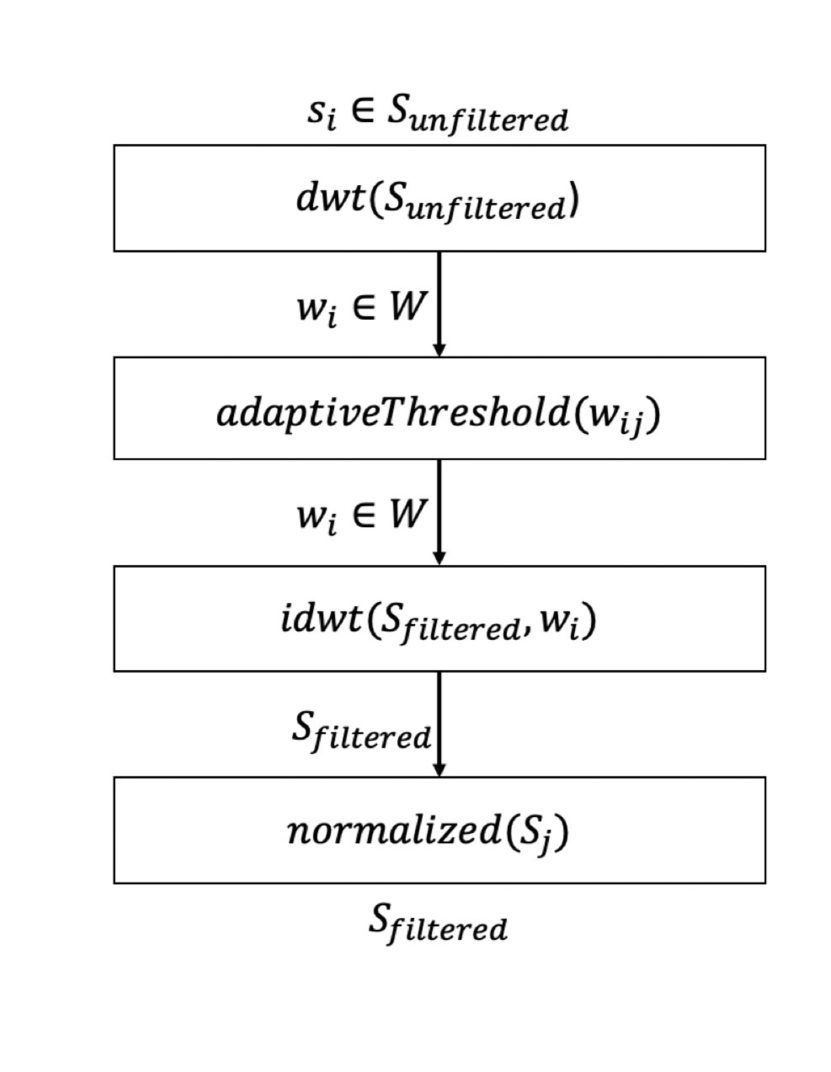
Figure 1: Progression of pre-processing $P:S\textsubscript{unfiltered}\mapsto P:S\textsubscript{filtered}$.

The procedure (3.1) outputs the denoised signal. The architecture of the Generative Adversarial Network (GAN) model (3.2) that inputs the pre-processed signal is subsequently detailed along with the signal-correlation analysis (5) performed on the model’s outputs. Then, the cardiovascular disease (CVD)-predictive model (3.4) that inputs the features identified by the signal-correlation analysis is described. Overall, the approach facilitates the evolution of an input of any 15s lead signal to the output of a CVD prediction. The approach is executed in Python 3.10 Van Rossum and Drake Jr (1995).

3.1 Pre-processing

Pre-processing takes each 15s electrocardiogram (ECG) lead signal as input S_unfiltered and denoises them (Algorithm 1). There are n_filters = 4 high-low pass Daubechie discrete wavelet transforms (dwtHP and dwtLP respectively) from the pywt 1.4.1 package Lee et al. (2022) performed. Upon completion of each dwt_i, the low pass signal cA_i is subsampled (resample) by two and passed to the next round of filters while the high pass signal cD_i is subsampled by two (resample) and extracted to become a wavelet (w_i). After all filters are applied, adaptive thresholding is performed on each of the i wavelets at each signal time point j with moving average window of length r = 32 Hazra and Byun (2020):

$$adaptiveThreshold(w_{ij})=$$ (1)

$$1/r\sum_{n=r*(j-1)}^{rj-1}\mid w_{1j}\mid\ *2^{i}$$

To construct the denoised signal, the inverse Daubechie DWT (idwt) function from the pywt 1.4.1 package Lee et al. (2022) is performed on the threshold-ed wavelets (w_i). These denoised signals (S) at each time point j are subsequently normalized to be between zero and one:

$$normalized(S_{j})=(S_{j}-min(S))/$$ (2)

$$(max(S)-min(S))$$

Examples of the pre-processing output are provided in (4.2).

Algorithm 1 Daubechie denoising algorithm

Input: S_unfiltered, n_filters
Output: S_filtered

1:$cA_{0}\leftarrow resample(dwtLP(S\textsubscript{unfiltered}))$

2:$cD_{0}\leftarrow dwtHP(S\textsubscript{unfiltered})$

3:$w_{0}\leftarrow resample(cD)$

4:for i=2 to n-1 do

5:     $cA_{i}\leftarrow resample(dwtLP(cA\textsubscript{i-1}))$

6:     $cD_{i}\leftarrow dwtHP(cA\textsubscript{i-1})$

7:     $w_{i}\leftarrow resample(cD_{i})$

8:end for

9:$w_{n}\leftarrow resample(cA\textsubscript{n-1})$

10:for i=2 to n do

11:     $w_{i}\leftarrow adaptiveThreshold(w_{i})$

12:end for

13:$S\textsubscript{filtered}\leftarrow idwt(w_{n},w\textsubscript{n-1})$

14:for i=n-2 down to 1 do

15:     $S\textsubscript{filtered}\leftarrow idwt(S\textsubscript{filtered},w\textsubscript{i})$

16:end for

3.2 GAN Model

Our GAN model consists of a bidirectional long short-term memory (LSTM) generator that aims to recreate ECG lead signals—from a two-signal input—that the discriminator cannot distinguish from the patient’s actual signal (Figure 2).

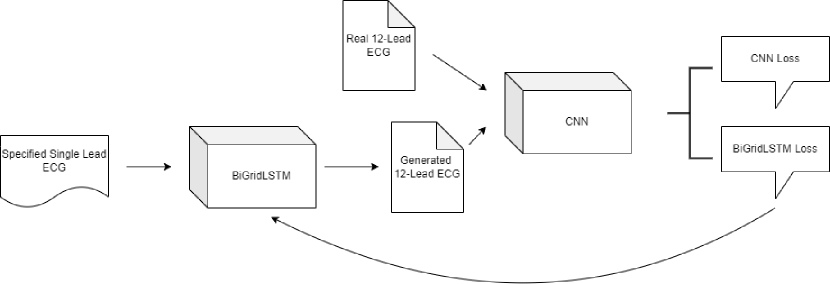
Figure 2: Overview of the GAN model. The generator is a bidirectional LSTM that takes a single lead input and the discriminator is a CNN that attempts to distinguish the real signal from the generated signal.

The discriminator of the GAN model is a convolutional neural network (CNN) that attempts to differentiate the artificial signals from the patients’ actual lead signals. Mathematically, the baseline GAN model can be modeled as a minmax game represented by the generator loss function—i.e., the penalties paid by either the generator or discriminator for failing to perform their respective tasks. The generator aims to minimize this loss while the discriminator attempts to maximize the loss for the generator. To mathematically represent the situation, the domain of all N pre-processed signals can be defined as ${s_{i}}\in S\textsubscript{filtered}$ while the M signals of the generator output, or in other words, the discriminator domain, are defined as ${q_{i}}\in Q$. The generator is thus a mapping defined as $G:S\textsubscript{filtered}\mapsto Q$. The loss function can then be defined as

$$\mathcal{L}(G,D,S\textsubscript{filtered},Q)=$$ (3)

$$min_{D}max_{G}\>\mathbb{E}_{q\sim p(q)}[log(D(q)]$$

$$+\mathbb{E}_{s\sim p(s)}[log(1-D(G(s)))]$$

where D is the discriminator, $\mathbb{E}_{q\sim p(q)}$ is the expectation of the probability given by the discriminator of a real signal being real on random input $p(q)$ over the distribution of ${q}$, and $\mathbb{E}_{s\sim p(s)}$ is the expectation of the probability given by the discriminator of a generated signal being real on random input $p(s)$ over the distribution of ${s}$ Zhu et al. (2017).

3.2.1 Bidirectional LSTM Generator

The baseline LSTM structure allows for long term dependencies to be considered in the model architecture. A LSTM is generally defined in terms of cell states which control what information is considered by the model through a series of gates. The sigmoid forget layer removes information from consideration, the sigmoidal input gate selects values of the cell state to be updated, the input hyperbolic tangent gate inputs new candidate values to the cell state, and finally sigmoidal and hyperbolic tangent output layers select the output information Hochreiter and Schmidhuber (1997). The cell state output is subsequently passed to the corresponding layer of the underlying recurrent neural network (RNN)—a type of neural network where the hidden layer outputs can be used to update prior layers—preserving the long term dependencies Sherstinsky (2020). This process is susceptible to the vanishing gradient problem: the gradient of the backpropagation updating the sigmoidal layers approaches zero due to the small derivatives at the sigmoid function extremes. The vanishing gradient problem prevents further model training. To prevent the gradient from vanishing, the baseline LSTM structure can be extended into a bidirectional grid. Instead of the information being passed from the hidden layers only temporally, the layers and corresponding cell states are stacked on top of each other to add a depth layer that decreases the probability that the backpropagation produces a near-zero gradient Schuster and Paliwal (1997). This more advanced, bidirectional grid approach is implemented as the generator $G:S\textsubscript{filtered}\mapsto Q$ according to the LSTM state variables, time block, and depth block outlined by Hazra and Byun (2020). The approach of Hazra and Byun (2020) is favored to the bidirectional LSTM-based ECG signal generator presented by Zhu et al. (2019) because of the explicit consideration of the vanishing gradient by Hazra and Byun (2020).

3.2.2 CNN Discriminator

The time-series nature of the ECG signal confers the use of one-dimensional convolutions in the CNN discriminator as opposed to the more traditional two-dimensional convolution used in computer vision Zhu et al. (2019). A one-dimensional CNN is modeled in terms the number and size (input and output) of its convolution and pooling layers, number of kernels per layer, and final activation function Kiranyaz et al. (2021) as defined for the discriminator here (Table 3). The kernels in each convolutional layer serve as feature filters that parse through both the generated and real ECG signals according to the defined stride length—computing the dot product between the kernel and signal while reducing the dimensions of the data Kiranyaz et al. (2019). Each kernel produces a feature map that represent certain characteristics of the ECG signal. To prevent over-fitting, the pooling layers sub-sample the feature maps. The final convolution produces a fully connected hidden layer whose outputs are subjected to the softmax activation function which gives the probability that the signal is generated or real Iwana et al. (2019). The probabilities are passed to the aforementioned loss function (Equation 3).

3.3 Cross-correlation analysis

The baseline signal correlation test is the cross-correlation function computed as

$$r(q,s)=\sum_{j=0}^{T}q_{j}s_{j}$$ (4)

where $q\in Q$ and $s\in S_{filtered}$ for all time points $T$ in the ECG signals Podobnik and Stanley (2008). For each of the 12 ECG leads, the cross-correlation function between every synthesized lead signal and the original patient signal is calculated and averaged across the entire data set. The function is subsequently charted and analyzed by cardiologists at the Robert Wood Johnson University Hospital for feature extraction. The efficiency of the feature extraction is compared to the studies by Ramli and Ahmad (2003), Chiu et al. (2005), and Lee et al. (2017b). While the cross-correlation function acts as a baseline mechanism for extracting the latent relationships learned by the GAN model, the auto-correlation function defined

$$r(q,i)=\sum_{j=i}^{T}q_{j}q_{j-i}$$ (5)

where $i$ is a time-translation introduced to the generated signal, may provide further, more definitive features Ramli and Ahmad (2003). This is because repeated, important patterns from each heartbeat should be perpetuated throughout the entirety of the signal which would only be captured by the auto-correlation function. The auto-correlation function is once again charted and analyzed by cardiologists at the Robert Wood Johnson University Hospital for feature extraction. The analysis done by Ramli and Ahmad (2003) serves as the baseline comparison.

3.4 CVD-Predictive CNN Model

We cannot write the approach for this section yet because it depends on how successful the aforementioned cross-correlation analysis is. Until we know what features are successfully identified, we cannot design a model structure; however, we include it here because the novelty of our research is not apparent without this model. We will implement it in the future. We anticipate using a CNN-predictive model as the models that have come closest to achieving multiple-CVD onset predictions are CNN-based models. That being said, the novelty of the analysis derives from utilizing all three components: using the GAN model to understand the latent relations of ECG signals, the cross-correlation analysis to identify the latent connections the GAN model is making, and the CVD-predictive model to predict multiple-CVD onsets which has never been done before successfully. The approach is generalizable as it can take any ECG input to train the GAN model, update the cross-correlation analysis, and fine-tune the CVD-predictive model. Furthermore, the ultimate aim of the approach is so that the resulting CVD-predictive model is generalizable for any ECG signal input and most CVD predictions.

4 Experiments

We implement our models in TensorFlow and experiment with three different generative models: our baseline GAN model, the one-lead predictive model by Seo et al. (2022), and our advanced bidirectional LSTM-1d CNN GAN model. All our models are evaluated on our dataset (4.1).

4.1 MyoVista Dataset

Our MyoVista dataset consists of 15s 12-lead ECG data measured using MyoVista’s wavECG patient data from three different hospitals: West Virginia University, Mount Sanai, and Windsor. Functional outcome data for each patient in the 1000-patient dataset is recorded. Patient ages ranged from 18-96 years old with a mean age of $56.8\pm{15}$ and patient gender is 46.6% and 53.4% female and male respectively. Each race is represented in the data set, but Caucasians are overrepresented (Table 1). Weight measurements (mean $86.8\pm{23}$kg) indicate a well-distributed sample with SD accounting for more than $25\%$ of the mean. The distribution of height (mean $169.5\pm{10}$cm) is more conservative but indicative of a distributed sample. Over 2000 functional outcomes are recorded—e.g., ejection fraction, Rsign, and blood pressure—for each patient. This dataset was collected because with a large array of functional outcomes, we expect to be able to extract features from the generated signals that can then be used to predict at least some of the functional outcomes. Furthermore, with MyoVista ECG signal data having been used to successfully predict CVD-onset in the past Sengupta et al. (2018a), signal data from the wavECG is used. Due to HIPAA regulations, other datasets cannot be accessed and therefore, the models are only evaluated on our dataset.

	Caucasian	African-American	Hispanic	Asian	Mean
%	80.5	5.7	3.7	6.3	NA
% Male	49.7	37.1	29.3	58.5	53.4
Age (years)	$\bf 56.7\pm{17}$	$53.1\pm{13}$	$53.4\pm{14}$	$50.6\pm{15}$	$56.8\pm{15}$
Weight (kg)	$89.2\pm{25}$	$\bf 93.2\pm{26}$	$79.8\pm{17}$	$68.1\pm{14}$	$86.8\pm{23}$
Height (cm)	$\bf 169.6\pm{10}$	$169.3\pm{10}$	$164.8\pm{8.7}$	$164.8\pm{8.4}$	$169.5\pm{10}$

Table 1: Percentage of MyoVista dataset represented by each race along with the racial breakdown of the generic patient data. The largest values for each category are bolded.

4.2 Pre-processing Validation

For each signal recorded by the wavECG, the pre-processing procedure outlined in Section 3.1 is performed. The denoised signals clearly display the correct number of heartbeats and fundamental components of a heartbeat: the P-Q segment, the QRS complex, and the S-T segment (Figure 3(b)). Furthermore, for each R-peak in the original signal (Figure 3(a)), there is an R-peak in the denoised signal (Figure 3(b)), further validating the correctness of the pre-processing procedure. Upon completion of the pre-processing procedure, the R-peak time intervals are calculated and each heartbeat is segmented. Padding is added to the signal according to the maximum R-peak time interval across all patients.

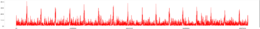
(a) Sub-figure 1. The original signal recorded by wavECG.

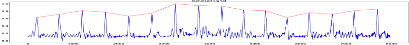
(b) Sub-figure 2. A representative denoised signal. The blue line is the result of the original signal being subjected to four high-low pass Daubechie discrete wavelet transforms, adaptive thresholding, four high-low pass Daubechie inverse wavelet transforms, and normalization as described in Section 3.1. The red line serves as proof that the algorithm is able to successfully identify each peak—i.e. R complex—of each heartbeat.

Figure 3: Comparison of the original signal recorded by wavECG and the denoised signal after the procedure outlined in Section 3.1 is performed.

Set	Total Number of Heartbeats	Heartbeats per Lead
Training	1,584,000	132,000
Validation	198,000	16,500
Test	198,000	16,500

Table 2: Data split for the GAN model inputs (Section 4.3)

For the GAN model (Section 4.3), the sequential time-series representation of each heartbeat constitutes the input. For each of the 1000 patients, there are 15 heartbeats. For each of the patient’s lead’s heartbeats, we are trying to predict the other 11 heartbeats; therefore, there are $1000*15*12*11=1,980,000$ model inputs. Because of the size of the pre-processed dataset, we randomly shuffled the heartbeats and allocated 80% for training, 10% for validation, and 10% for training (Table 2).

4.3 Generation of ECG signals

To reiterate, we train a basic LSTM generator and one-layer 1d-CNN discriminator for our baseline GAN model. We then compare the results to our advanced GAN model with the bidirectional LSTM generator and multi-layer 1d-CNN discriminator optimized for each lead. Both of these results are subsequently compared to Seo et al. (2022) GAN model that was specifically designed to synthesize the signals from just one lead. Note we did not have the requisite time to the model from the Seo et al. (2022) study, but instead only present it here as a data point. In the future, we will reconstruct the model and test it on our dataset and compare the results to our model.
To evaluate how similar the generated signal is to the input signal, we use Fréchet Distance (FD) defined as:

$$FD(s\in S_{filtered},q\in Q)=$$ (6)

$$min(max_{i=1,...,n}(||s_{i},q_{i}||))$$

where $||s_{i},q_{i}||$ is the Euclidean distance between points $s_{i}$ and $q_{i}$. In other words, FD computes the maximum distance of $s_{i}$ and $q_{i}$ in a given alignment for all alignments of n points from s and from q and then finds the minimum of these maximum distances. Therefore, FD evaluates similarity based on both the ordering and location of the signals’ points. Both factors are considered in the cross-correlation analysis (5), thus FD is the chosen similarity metric. Because the model proposed by Seo et al. (2022) is specifically designed for the limb lead I as the sole input, the individual FD scores for this model will likely not be as low, but comparable—i.e., within one standard deviation.
Our baseline model is trained for nine epochs using the learning rate of $1\mathrm{e}{-4}$. Note that because we did not have enough time to optimize hyperparameters, we did not optimize the learning rate but we did optimize the number of epochs. We saved the model after each epoch so that the epoch that produced the lowest FD during validation could be selected for the generation. Epoch 1 was selected because it produced the lowest FD score in the validation (Figure 4).

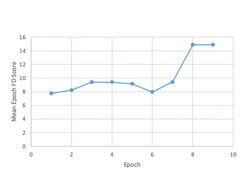
Figure 4: The model’s mean FD score on the validation score after each epoch.

The input batch size was 256. Cross-entropy was used as the loss function and the Adam algorithm was used as our optimizer. For the bidirectional LSTM generator, a time-distributed 1-unit dense layer with a sigmoidal activation was applied. The details of the CNN discriminator are presented in Table 3. The Relu activation function is used for the convolution and final convolution (FC) layers.

Layer	Number of Kernels	Filter Size	Stride
$C_{1}$	64	3	3
$P_{1}$	1	2	2
$C_{...}$	64	3	3
$P_{...}$	1	2	2
FC	100	1	1
Softmax	1	1	1

Table 3: The definition of each CNN layer of the GAN discriminator

The mean FD scores comparing our baseline model and the one-lead model created by Seo et al. (2022) are presented in Table 4. Our baseline model outperforms the model by Seo et al. (2022) in two of the three experiments. Further inspection of the experiments by Seo et al. (2022) indicates FD scores for the limb leads that are far lower than ours but far higher FD scores for the pre-cordial leads. Biologically, this can be explained by visualizing our prediction (Figure 5). Our generated signal clearly preserves all of the fundamental components of a heartbeat: the P-Q segment, the QRS complex, and the S-T segment. These fundamental components of the heartbeat are better preserved in the pre-cordial leads as they are closer to the heart; therefore, it appears that our model is trained better to generate the pre-cordial signals than it is to the limb leads. This could be explained by the noisiness of the limb leads prior to pre-processing. The limb leads were noticeably more noisy before the pre-processing and although the signals were processed successfully, the QPRST components were less distinct for the limb leads than the pre-cordial leads.

Metric	Baseline	Seo et al. (2022) E1	Seo et al. (2022) E2	Seo et al. (2022) E3
FD	7.77	9.062	8.124	6.071

Table 4: Mean FD scores from our baseline model, our advanced model, and the three experiments that Seo et al. (2022) used.

Figure 5: Representative generated signal by the baseline model. Each heartbeat of the signal clearly contains the P-Q segment, the QRS complex, and the S-T segment.

4.4 Features of ECG Signals that Predict CVD

	1	2	3
1	N/A	0.53	-0.33
2	0.53	N/A	0.48
3	-0.33	0.48	N/A
4	-0.83	-0.88	-0.11
5	0.80	0.05	-0.77
6	0.14	0.86	0.82
7	-0.38	-0.35	-0.01
8	0.02	-0.08	-0.15
9	0.30	0.29	0.02
10	0.45	0.46	0.06
11	0.55	0.52	0.01
12	0.57	0.53	0.01

(a) Sub-table 1. Precordial leads 1-3

	4	5	6
1	-0.83	0.80	0.14
2	-0.88	0.05	0.86
3	-0.11	-0.77	0.82
4	N/A	-0.42	-0.56
5	-0.42	N/A	-0.35
6	-0.56	-0.35	N/A
7	0.43	-0.18	-0.19
8	0.06	0.15	-0.10
9	-0.30	0.22	0.22
10	-0.49	0.28	0.33
11	-0.58	0.35	0.33
12	-0.60	0.37	0.34

(b) Sub-table 2. Precordial leads 4-6

Table 5: The average correlation coefficient between each of the first three precordial leads signals (Table 5(a)) and the other eleven leads. The average correlation coefficient between each of the other precordial leads signals of IV, V, and VI (Table 5(b)) and the other eleven leads. All patient data were included in the calculations.

To determine baseline relationships between the more informative precordial leads—i.e., the leads positioned next to the heart—and the other leads, the average correlation coefficient between each precordial lead and the other remaining eleven leads is calculated with consideration of all patients in the study prior to pre-processing (Table 5). The correlation coefficients taken here initially will eventually then be compared to the correlation coefficient results of the generated GAN model signals. Note that because this was a part of Max’s individual project and we barely had enough time to finish the group experiment during this time (we are using our group member’s GPU and we could not get time to perform the analysis) we could not repeat the analysis for the generated signals. This section is included once again to address the novelty of the project and will be completed for the final publication.

4.5 Validation of Multiple-CVD Predictions

This section is included once again to address the novelty of the project and will be completed for the final publication.

5 Analysis

In order to understand the biological underpinnings of the model’s performance and to assess the model’s performance in predicting the signals of specific leads, we split the validation and testing sets in terms of the predicted lead to produce the advanced model. In other words, we train 12 generators (and consequently 12 discriminators) which are each specialized in generating a particular lead. For each predicted lead, the epoch that performed best on the development set corresponding to that lead is used on the test set for that lead (Figure 6). The batch size for the advanced model is 128.

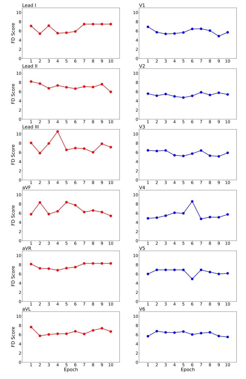
Figure 6: The model’s mean FD score on the validation set for the generated signal of each lead after each of the ten epochs. The mean FD scores for six limb leads (red) are on the left and the six pre-cordial leads (blue) are on the right. The best epoch for each lead is subsequently chosen (Table 6).

5.1 Performance Analysis

In Table 6, the mean FD score of each lead’s best model’s performance on the testing set is compared to the best mean FD score of Seo et al. (2022). While our model’s overall mean FD score of $6.38\pm{0.1}$ outperforms all three of Seo et al. (2022) models’ mean FD scores, further inspection of the specific leads in which our model performs better yields a distinct trend. For each of the limb leads (Table 6(a)), Seo et al. (2022) outperforms our model. Specifically, the signals generated for aVR and aVL by their model are much more similar to the patient’s actual signal than our model; however, when examining the pre-cordial leads (Table 6(b)), our model consistently outperforms for every lead. When comparing within our model, only one of the two limb leads (AVR and AVF) better the worst performing pre-cordial lead (V6), and neither outperforms any of the other pre-cordial leads. This differentiation in model performance between the limb and pre-cordial leads perhaps can be explained by three different explanations: biological, mechanical, and computational.

	I	II	III	aVR	aVL	aVF
Epoch	1	9	1	9	3	1
Mean FD	5.76	6.28	5.74	5.45	7.06	5.50
Seo et al. (2022) FD	NA	4.55	4.93	0.94	1.48	5.25

(a) Sub-table 1. Limb leads

	V1	V2	V3	V4	V5	V6
Epoch	8	4	8	6	5	9
Mean FD	4.73	4.89	5.18	4.77	4.71	5.55
Seo et al. (2022) FD	13.64	10.85	17.64	15.27	13.60	11.50

(b) Sub-table 2. Pre-cordial leads

Table 6: The epoch producing the best FD score of each lead that is subsequently used in the prediction of that lead’s signal is presented. The mean FDs from the model’s prediction of each lead are then calculated and compared to the mean FD from Seo et al. (2022) for each lead. Lead I is omitted from Seo et al. (2022) because their model is designed to take lead I as input. The better mean FD of the two models is bolded.

From a biological perspective, limb lead position is less defined amongst physicians Tung (2021), and thus, since the MyoVista dataset (4.1) was collected from multiple hospitals across multiple states, the positioning preferences between physicians could interfere with the model’s ability to pinpoint predictive heuristics. Furthermore, the wavECG used to record the patient signals for the MyoVista dataset was designed to be able to identify left ventricular diastolic dysfunction or LVDD Sengupta et al. (2018a). LVDD is characterized by p-wave dispersion which is more identifiable in abnormalities in pre-cordial leads Taha et al. (2016). Consequently, the wavECG hardware may have been implicitly designed to be more sensitive to the pre-cordial leads and thus the model may be able to identify more well-defined features in those leads as opposed to the limb leads. Computationally, following the application of the pre-processing procedure (3.1) the denoised samples of our pre-cordial leads contain better-defined PQRST wave characteristics along with less noise overall when compared to the limb leads (Figure 7). In particular, the P-wave is far more defined in each heartbeat of the pre-cordial lead (Figure 7(b)) which also provides further credence to the aforementioned argument that the wavECG is more sensitive to the pre-cordial leads.

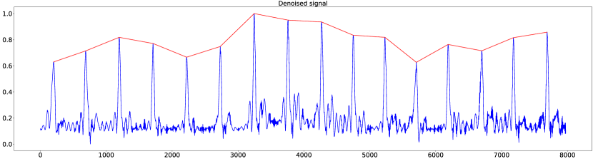
(a) Sub-figure 1. Denoised limb lead representative sample

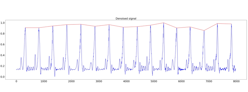
(b) Sub-figure 1. Denoised pre-cordial lead representative sample

Figure 7: Comparison of a representative denoised limb lead signal and a representative pre-cordial lead signal.

5.2 Error Analysis

To understand the trends the model identifies in each lead and the inability of the model to reproduce all characteristics of the PQRST complex, we detailed manual error analysis of predictive examples from the lead best-predicted by the model (V5), the lead worst-predicted by the model (AVL), and a representative lead (V1). The lead for which the model performs the best for, V5, simply captures the downslope of the R peak and no other feature (Figure 8).

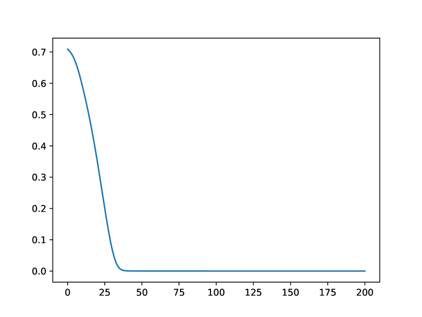
Figure 8: A representative sample of a generated V5-lead signal. The V5 had the best mean predicted FD score during testing but fails to capture any PQRST complex features.

This points to flaws in the FD score as the only metric to validate and test the model. Comparatively, the worst-predicted lead by the model, AVL, captures more features, notably a P-wave; however, it seems to predict multiple heartbeats instead of the intended single heartbeat (Figure 9). In this context, the depth dimension of the bidirectional LSTM generator (3.2) appears to fail in differentiating between the heights of the P-wave peak, R-peak, and T-wave peak.

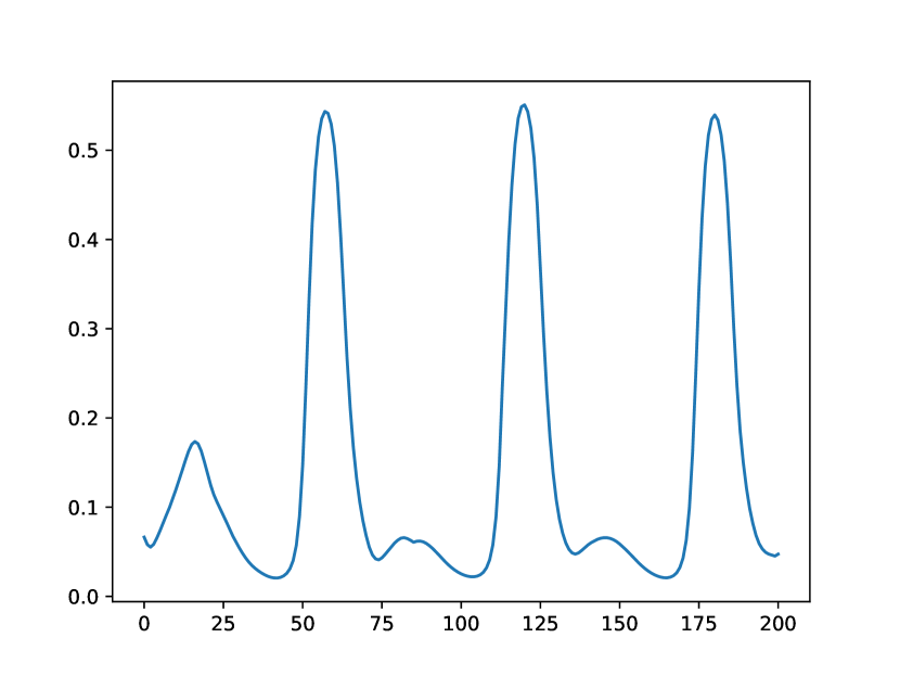
Figure 9: A representative sample of a generated AVL-lead signal. The AVL-lead had the worst mean predicted FD score during testing and incorrectly generates heartbeats that have P-wave and T-wave peak magnitudes comparable to the R-peak.

The V1 lead, on the other hand, captures multiple features along with representing only one heartbeat despite having a middling FD score (Figure 10). The generated signal contains not only the down-slope of the previous R peak but a clear P-wave whose peak is accurately diminished compared to the predicted heartbeat’s R peak; however, it still does not capture the T-wave. This can be attributed to the extensive zero-value padding that is sometimes appended to the end of each of the denoised signals (3.1) in order to make all the heartbeats the same length for model input. Since the T-wave peaks’ magnitudes are generally dampened in comparison to the P-wave peaks and R-peak Costa et al. (2021), the model could mischaracterize the T-wave as signal noise and thus the generator perhaps never learned how to generate the T-wave. This could also point to flaws in our denoising procedure. Note I could not find a way to provide distributions of the categorized errors in a figure (see below) because the automatic identification of the components of the PQRST complexes themselves would require the training of an entirely new deep learning model; however, for publication, I will try to annotate as many of the figures as possible.

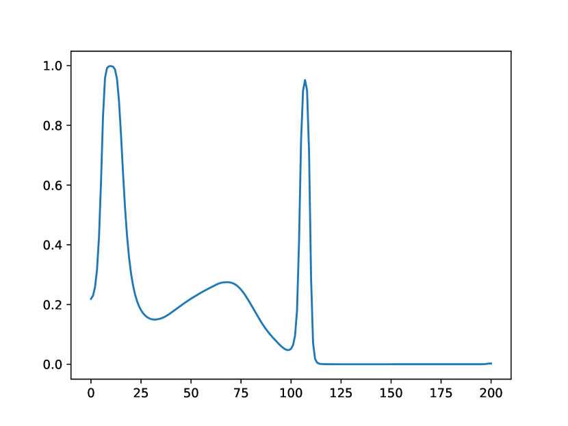
Figure 10: A representative sample of a generated V1-lead signal. Out of all the generated signals, the V1 correctly preserves the most PQRST signals, most notably a dampened P-wave and a distinct R-peak.

5.3 Future Directions

Because of the inability of the model to consistently and correctly characterize the necessary components of the PQRST complex for every lead, the model can be improved in future work in order to eventually identify conserved features that can be used as an input to a CVD-predictive model. This can be done by correcting the identified limitations mentioned in Section 5.2. Foremost, the model is limited because we did not optimize the pre-processing algorithm—most notably the denoising algorithm—and thus a more advanced pre-processing algorithm could perhaps denoise the signal better such that the T-wave is not lost in signal generation. Although many previous generative and predictive models that take ECG signal inputs employ Daubechie discrete wavelet transforms (DWT) Hazra and Byun (2020); Singh and Pradhan (2021), other models incorporate other methods. For example, Zhu et al. (2019) employs a variational autoencoder to correctly capture the distribution of data before performing a DWT-like procedure. Perhaps by training, validating, testing, and comparing multiple models that each take signals with a different pre-processing procedure performed, an optimal procedure can be identified and implemented so that more PQRST complex features are not misinterpreted as noise during model training. Furthermore, heartbeats with R-peak differentials that can be classified as statistical outliers can be eliminated in order to prevent extensive zero-padding to the segmented ECG signals which could also aid with T-wave preservation. This would also remove the need for the resampling we perform to reduce the input shape of the input layers of the bidirectional LSTM. By allocating time to tuning the hyperparameters of the bidirectional LSTM, perhaps the depth layers can effectively generate P-wave and T-wave peaks with the correct magnitudes. Finally, our analysis also hints at the flaws in Fréchet Distance as the evaluation metric for ECG signal generation and we will attempt to construct a novel evaluation metric. The hallmark of an accurately generated signal is the preservation of the PQRST complex and perhaps a metric that also measures the generated heartbeat’s similarity to a standardized PQRST complex will prove successful.

6 Conclusion

We present ECGNet that ultimately improves the accuracy of CVD-onset predictions by first improving the generation of a complete 12-lead ECG set from a single ECG lead signal input. Our generative adversarial network (GAN) model shows state-of-the-art accuracy in the generation of the pre-cordial lead signals—preserving distinct elements of the heartbeat’s PQRST complex electrical signals. By applying cross-correlation analysis on ECGNet’s GAN model’s generated signals, latent features essential to the generation of accurate signals, and thus fundamental to the classification of CVD-onset, are identified. Note that the cross-correlation analysis and predictive CNN model were a part of Max’s personal project and could not be completed during the semester’s time frame; however, we chose to write about it hypothetically in the conclusion because it will be in the final publication and is essential in justifying the need for the project. Because of the identification of these hidden features, ECGNet allows cardiology to overcome the previous black box barriers that prevented the prediction of multiple-CVD targets. All our resources besides the dataset (due to HIPAA protections), but including models and source codes, are available through our open-source project at https://github.com/maxbagga/ScarletEagle1. Despite a decent performance, the GAN model still underperforms other state-of-the-art models in the generation of limb lead signals. We plan to tackle this challenge by collecting a second data set to train the limb lead generation with a different, non-MyoVista waveECG device. This will supplement the strengths of the waveECG in producing clearer pre-cordial lead signals while compensating for its tendencies to produce more noisy limb lead signals. Then, we will optimize pre-processing methods to give better limb lead inputs by experimenting with different denoising techniques and employing variational autoenconders to first capture the distribution of the data. Finally, we will aim to develop a new evaluation metric that considers the preservation of the PQRST complex in evaluating the accuracy of signal generation as the current metric employed—Fréchet Distance (FD)—only evaluates the location and orderings of signal points. Consequently, the leads with generated signals preserving the most PQRST complex elements often have middling FD scores which, with a novel method, will be rectified.

References

- Burguera (2019) Antoni Burguera. 2019. Fast qrs detection and ecg compression based on signal structural analysis. volume 23, pages 123–131.
- Chiou et al. (2021) YA Chiou, JY Syu, SY Wu, Lian-Yu Lin, Li Tzu Yi, Ting-Tse Lin, and Shien-Fong Lin. 2021. Electrocardiogram lead selection for intelligent screening of patients with systolic heart failure. In Scientific Reports Volume 11(1948), page NA, London, United Kingdom. Nature Research.
- Chiu et al. (2005) Chuang-Chien Chiu, Tong-Hong Lin, and Ben-Yi Liau. 2005. Using correlation coefficient in ecg waveform for arrhythmia detection. Biomedical Engineering: Applications, Basis and Communications, 17(03):147–152.
- Costa et al. (2021) Renan Costa, Thaís Winkert, Aline Manhães, and João Paulo Teixeira. 2021. Qrs peaks, p and t waves identification in ecg. Procedia Computer Science, 181:957–964. CENTERIS 2020 - International Conference on ENTERprise Information Systems / ProjMAN 2020 - International Conference on Project MANagement / HCist 2020 - International Conference on Health and Social Care Information Systems and Technologies 2020, CENTERIS/ProjMAN/HCist 2020.
- Craven et al. (2017) Darren Craven, Brian McGinley, Liam Kilmartin, Martin Glavin, and Edward Jones. 2017. Adaptive dictionary reconstruction for compressed sensing of ecg signals. volume 21, pages 645–654.
- Dawber et al. (1952) TR Dawber, WB Kannel, DE Love, and RB Streeper. 1952. The electrocardiogram in heart disease detection a comparison of the multiple and single lead procedures. In Circulation Volume V, pages 559–566, NA. Lippincott Williams & Wilkins.
- Drew et al. (2002) Barbara J. Drew, Michele M. Pelter, Donald E. Brodnick, Anil V. Yadav, Debbie Dempel, and Mary G. Adams. 2002. Comparison of a new reduced lead set ecg with the standard ecg for diagnosing cardiac arrhythmias and myocardial ischemia. In Journal of Electrocardiology Volume 35(4B), pages 13–21, NA. Elsevier.
- Dutta et al. (2020) Aniruddha Dutta, Tamal Batabyal, Meheli Basu, and Scott T. Acton. 2020. An efficient convolutional neural network for coronary heart disease prediction. Expert Systems with Applications, 159:113408.
- Ebrahimi et al. (2020) Zahra Ebrahimi, Mohammad Loni, Masoud Daneshtalab, and Arash Gharehbaghi. 2020. A review on deep learning methods for ecg arrhythmia classification. In Expert Systems with Applications: X Volume 7, page NA, NA. Elsevier.
- Grande-Fidalgo et al. (2021) Alejandro Grande-Fidalgo, Javier Calpe, Mónica Redón, Carlos Millán-Navarro, and Emilio Soria-Olivas. 2021. Lead reconstruction using artificial neural networks for ambulatory ecg acquisition. volume 21.
- Hazra and Byun (2020) Debapriaya Hazra and Yung-Cheol Byun. 2020. Synsiggan: Generative adversarial networks for synthetic biomedical signal generation. In Biology Volume 9(12), page NA, NA. Multidisciplinary Digital Publishing Institute.
- He et al. (2018) Jinyuan He, Le Sun, Jia Rong, Hua Wang, and Yanchun Zhang. 2018. A pyramid-like model for heartbeat classification from ecg recordings. volume 13.
- Hochreiter and Schmidhuber (1997) Sepp Hochreiter and Jürgen Schmidhuber. 1997. Long Short-Term Memory. Neural Computation, 9(8):1735–1780.
- Hsu and Wu (2014) Chih-Hao Hsu and Sau-Hsuan Wu. 2014. Robust signal synthesis of the 12-lead ecg using 3-lead wireless ecg systems. In 2014 IEEE International Conference on Communications (ICC), pages 3517–3522.
- Iwana et al. (2019) Brian Kenji Iwana, Ryohei Kuroki, and Seiichi Uchida. 2019. Explaining convolutional neural networks using softmax gradient layer-wise relevance propagation. In 2019 IEEE/CVF International Conference on Computer Vision Workshop (ICCVW), pages 4176–4185.
- Kachuee et al. (2018) Mohammad Kachuee, Shayan Fazeli, and Majid Sarrafzadeh. 2018. Ecg heartbeat classification: A deep transferable representation. In 2018 IEEE International Conference on Healthcare Informatics (ICHI), pages 443–444.
- Kiranyaz et al. (2021) Serkan Kiranyaz, Onur Avci, Osama Abdeljaber, Turker Ince, Moncef Gabbouj, and Daniel J. Inman. 2021. 1d convolutional neural networks and applications: A survey. Mechanical Systems and Signal Processing, 151:107398.
- Kiranyaz et al. (2019) Serkan Kiranyaz, Turker Ince, Osama Abdeljaber, Onur Avci, and Moncef Gabbouj. 2019. 1-d convolutional neural networks for signal processing applications. In ICASSP 2019 - 2019 IEEE International Conference on Acoustics, Speech and Signal Processing (ICASSP), pages 8360–8364.
- Lee et al. (2022) Gregory Lee, Ralf Gommers, Kai Wohlfahrt, Filip Wasilewski, Aaron O’Leary, Holger Nahrstaedt, Alexandre Sauvé, Ankit Agrawal, Daniel M. Pelt, Helder Oliveira, Thomas Arildsen, Christian Clauss, Frank Yu, Matthew Brett, Michel Pelletier, SylvainLan, Daniele Tricoli, Saket Choudhary, asnt, Arfon Smith, 0-tree, Balint Reczey, Corey Goldberg, Daniel Goertzen, Dawid Laszuk, ElConno, Jacopo Antonello, Jakub Mandula, jakirkham, and Jonathan Dan. 2022. Pywavelets/pywt: v1.4.1.
- Lee et al. (2017a) Hong J. Lee, Dong S. Lee, Hyun B. Kwon, Do Y. Kim, and Kwang S. Park. 2017a. Reconstruction of 12-lead ecg using a single-patch device. volume 56, page 319–327.
- Lee et al. (2017b) Jaewon Lee, Jinwoo Kim, and Miyoung Shin. 2017b. Correlation analysis between electrocardiography (ecg) and photoplethysmogram (ppg) data for driver’s drowsiness detection using noise replacement method. Procedia Computer Science, 116:421–426. Discovery and innovation of computer science technology in artificial intelligence era: The 2nd International Conference on Computer Science and Computational Intelligence (ICCSCI 2017).
- Li and Boulanger (2020) Hongzu Li and Pierre Boulanger. 2020. A survey of heart anomaly detection using ambulatory electrocardiogram (ecg). In Sensors Volume 20(5), page NA, NA. Multidisciplinary Digital Publishing Institute.
- Mir and Singh (2021) Haroon Yousuf Mir and Omkar Singh. 2021. Ecg denoising and feature extraction techniques – a review. volume 45, pages 672–684. Taylor & Francis. PMID: 34463593.
- Oosterom (2002) A. van Oosterom. 2002. Solidifying the solid angle. In Journal of Electrocardiology Volume 35(4), pages 181–192, NA. Elsevier.
- Podobnik and Stanley (2008) Boris Podobnik and H. Eugene Stanley. 2008. Detrended cross-correlation analysis: A new method for analyzing two nonstationary time series. Phys. Rev. Lett., 100:084102.
- Ramli and Ahmad (2003) A.B. Ramli and P.A. Ahmad. 2003. Correlation analysis for abnormal ecg signal features extraction. In 4th National Conference of Telecommunication Technology, 2003. NCTT 2003 Proceedings., pages 232–237.
- Roth et al. (2020) GA Roth, GA Mensah, CO Johnson, G Addolorato, E Ammirati, LM Baddour, NC Barengo, AZ Beaton, EJ Benjamin, CP Benzinger, A Bonny, M Brauer, M Brodmann, TJ Cahill, J Carapetis, AL Catapano, SS Chugh, LT Cooper, J Coresh, M Criqui, N DeCleene, KA Eagle, S Emmons-Bell, VL Feigin, J Fernández-Solà, G Fowkes, E Gakidou, SM Grundy, FJ He, G Howard, F Hu, L Inker, G Karthikeyan, N Kassebaum, W Koroshetz, C Lavie, D Lloyd-Jones, HS Lu, A Mirijello, AM Temesgem, A Mokdad, AE Moran, P Muntner, J Narula, B Neal, M Ntsekhe, G Moraes de Oliveira, C Otto, M Owolabi, M Pratt, S Rajagopalan, M Reitsma, ALP Ribeiro, N Rigotti, A Rodgers, C Sable, S Shakil, K Sliwa-Hahnle, B Stark, J Sundström, P Timpel, IM Tleyjeh, M Valgimigli, T Vos, PK Whelton, M Yacoub, L Zuhlke, C Murray, and V Fuster. 2020. Global burden of cardiovascular diseases and risk factors, 1990–2019. In Journal of the American College of Cardiology Volume 76 (25), pages 2982–3021, NA. Elsevier.
- Sajja and Kalluri (2020) Tulasi Krishna Sajja and Hemantha Kumar Kalluri. 2020. A deep learning method for prediction of cardiovascular disease using convolutional neural network. Revue d’Intelligence Artificielle, 34(5):601–606.
- Schuster and Paliwal (1997) M. Schuster and K.K. Paliwal. 1997. Bidirectional recurrent neural networks. IEEE Transactions on Signal Processing, 45(11):2673–2681.
- Sengupta et al. (2018a) Partho P. Sengupta, Hemant Kulkarni, and Jagat Narula. 2018a. Prediction of abnormal myocardial relaxation from signal processed surface ecg. Journal of the American College of Cardiology, 71(15):1650–1660.
- Sengupta et al. (2018b) Partho P. Sengupta, Hemant Kulkarni, and Jagat Narula. 2018b. Prediction of abnormal myocardial relaxation from signal processed surface ecg. Journal of the American College of Cardiology, 71(15):1650–1660.
- Seo et al. (2022) Hyo-Chang Seo, Gi-Won Yoon, Segyeong Joo, and Gi-Byoung Nam. 2022. Multiple electrocardiogram generator with single-lead electrocardiogram. volume 221, page 106858.
- Shankar et al. (2020) VirenViraj Shankar, Varun Kumar, Umesh Devagade, Vinay Karanth, and K. Rohitaksha. 2020. Heart disease prediction using cnn algorithm. SN Computer Science, 1(3).
- Sherstinsky (2020) Alex Sherstinsky. 2020. Fundamentals of recurrent neural network (rnn) and long short-term memory (lstm) network. Physica D: Nonlinear Phenomena, 404:132306.
- Singh and Pradhan (2021) Pratik Singh and Gayadhar Pradhan. 2021. A new ecg denoising framework using generative adversarial network. volume 18, pages 759–764.
- Sohn et al. (2020) Jangjay Sohn, Seungman Yang, Yunseo Lee, Joonnyong Ku, and Hee Chan Kim. 2020. Reconstruction of 12-lead electrocardiogram from a three-lead patch-type device using a lstm network. In Sensors Volume 20(11), page NA, NA. Multidisciplinary Digital Publishing Institute.
- Stracina et al. (2022) Tibor Stracina, Marina Ronzhina, Richard Redina, and Marie Novakova. 2022. Golden standard or obsolete method? review of ecg applications in clinical and experimental context. In Frontiers in Physiology Volume, page NA, NA. Frontiers Media S.A.
- Taha et al. (2016) Tamer Taha, Khaled Sayed, Mohamad Saad, and Mohammed Samir. 2016. How accurate can electrocardiogram predict left ventricular diastolic dysfunction? The Egyptian Heart Journal, 68(2):117–123.
- Toyoshima et al. (1958) Hideo Toyoshima, Hiroshi Kato, Takehiko Isobe, Yoshio Kutsuna, Teruo Nagaya, and Yoshiko Saruhashi. 1958. Electrocardiogram and vectorcardiogram reconstruction and its application to clinical diagnosis of myocardial infarction. In American Heart Journal Volume 56(2), pages 165–194, NA. Elsevier.
- Tung (2021) Robert T Tung. 2021. Electrocardiographic limb leads placement and its clinical implication: Two cases of electrocardiographic illustrations. Kans J Med, 14:229–230.
- Ulloa-Cerna et al. (2022) Alvaro Ulloa-Cerna, Linyuan Jing, John Pfeifer, Sushravya Raghunath, Jeffrey Ruhl, Daniel Rocha, Joseph Leader, Noah Zimmerman, Greg Lee, Christopher Steinhubl, Steven Good, Christopher Haggerty, and Brandon Fornwalt. 2022. rechommend: An ecg-based machine learning approach for identifying patients at increased risk of undiagnosed structural heart disease detectable by echocardiography. In Circulation Volume 146(1), pages 36–47, NA. Lippincott Williams & Wilkins.
- Van Rossum and Drake Jr (1995) Guido Van Rossum and Fred L Drake Jr. 1995. Python reference manual. Centrum voor Wiskunde en Informatica Amsterdam.
- Weimann and Conrad (2021) Kuba Weimann and Tim O. Conrad. 2021. Transfer learning for ecg classification. Scientific Reports, 11(1).
- Wu et al. (2021) Mengze Wu, Yongdi Lu, Wenli Yang, and Shen Yuong Wong. 2021. A study on arrhythmia via ecg signal classification using the convolutional neural network. Frontiers in Computational Neuroscience, 14.
- Zhou et al. (2021) Liye Zhou, Zhifei Guo, Bijue Wang, Yongqin Wu, Zhi Li, Hongmei Yao, Ruiling Fang, Haitao Yang, Hongyan Cao, and Yuehua Cui. 2021. Risk prediction in patients with heart failure with preserved ejection fraction using gene expression data and machine learning. In Frontiers in Genetics, page NA, NA. Frontiers Media S.A.
- Zhu et al. (2019) Fei Zhu, Fei Ye, Yuchen Fu, Quan Liu, and Bairong Shen. 2019. Electrocardiogram generation with a bidirectional lstm-cnn generative adversarial network. In Scientific Reports Volume 9 (6374), page N/A, London, United Kingdom. Nature Research.
- Zhu et al. (2017) Jun-Yan Zhu, Taesung Park, Phillip Isola, and Alexei A. Efros. 2017. Unpaired image-to-image translation using cycle-consistent adversarial networks. In 2017 IEEE International Conference on Computer Vision (ICCV), pages 2242–2251.