A High-Performance Design, Implementation, Deployment,
and Evaluation of The Slim Fly Network

Abstract

Novel low-diameter network topologies such as Slim Fly (SF) offer significant cost and power advantages over the established Fat Tree, Clos, or Dragonfly. To spearhead the adoption of low-diameter networks, we design, implement, deploy, and evaluate the first real-world SF installation. We focus on deployment, management, and operational aspects of our test cluster with 200 servers and carefully analyze performance. We demonstrate techniques for simple cabling and cabling validation as well as a novel high-performance routing architecture for InfiniBand-based low-diameter topologies. Our real-world benchmarks show SF’s strong performance for many modern workloads such as deep neural network training, graph analytics, or linear algebra kernels. SF outperforms non-blocking Fat Trees in scalability while offering comparable or better performance and lower cost for large network sizes. Our work can facilitate deploying SF while the associated (open-source) routing architecture is fully portable and applicable to accelerate any low-diameter interconnect.

1 INTRODUCTION

Low-diameter network topologies such as Slim Fly (SF) [1] have gained significant traction during the last decade. Initial designs in that line of work, Dragonfly (DF) [2] and Flattened Butterfly [3], both with diameter three, focused on improving latency and physical layout. After that, SF lowered the diameter to two, based on an observation that low-diameter does not only improve performance by reducing end-to-end latencies, but it also reduces cost and power consumption. This is because, when the diameter is lower, packets on average traverse fewer switches, switch buffers, and links. Thus, fewer links and buffers are needed to construct the network (for a fixed bandwidth), and less dynamic power is needed for moving the packets through the network.

SF’s construction costs, consumed power, and latency are lower than those of Clos and Fat Tree (FT) by respectively, $\approx$25-30%, $\approx$25-30%, and $\approx$50%. However, SF has still not seen a real physical deployment, and it is uncertain how to deploy SF in practice. To spearhead the practical development of low-diameter networks and show the state-of-the-practice, we design, implement, deploy, and evaluate the first SF installation that includes switches and endpoints, as shown in Fig. A High-Performance Design, Implementation, Deployment, and Evaluation of The Slim Fly Network. We discuss the encountered challenges, and we show that the construction process is straightforward and comparable to established designs such as Clos.

Moreover, to maximize performance benefits from using SF, we design and implement a novel high-performance multipath routing scheme for general low-diameter networks, and we install and use it with the deployed SF cluster. Our routing shows superior performance over the state-of-the-art, and it is independent of the underlying topology details and of the interconnect architecture. Thus, it could be portably used on different topologies (e.g., Xpander [4]) and on different architectures (e.g., Ethernet or InfiniBand [5]).

Figure 2: The structure of a small example Fat Tree (FT), Dragonfly (DF), and Slim Fly (SF), and the corresponding installations. Each topology comes with a modular design, where switches form groups (SF, DF) or pods (FT). Such groups can become racks in a physical installation.

The equipment available to us is based on the InfiniBand (IB) architecture [5]. IB enables a high-speed switched fabric with hardware (HW) support for remote direct memory access (RDMA) [6, 7]. IB is widely used in high-performance systems, for example four out of ten most powerful systems in the Top500 list (Jun. 2023 issue) [8], manufactured by IBM, Nvidia, and Atos, use the IB interconnect. We use our routing protocol with the IB networking stack; our whole implementation is publicly available to foster future research into multipath routing. Importantly, we provide the first multipathing for IB that can use arbitrary paths (including non-minimal and disjoint ones) and that is independent of the structure details of the underlying network [9, 10].

In our evaluation, we consider a broad range of communication-intense applications that represent traditional dense computations (like physics simulations), sparse graph processing [11, 12, 13, 14, 15, 16], deep neural network (DNN) training [17, 18, 19], and a number of microbenchmarks testing particular popular communication patterns. Our results showcase that SF delivers high performance while achieving optimal, or near optimal scalability, which directly translates to low construction costs. To further reinforce these outcomes, we also conduct a comprehensive comparison between SF and a non-blocking FT that we deploy using the same hardware. Here, SF offers comparable or better performance to FT in a majority of used applications. Simultaneously, its superior scalability ensures up to 50% cost improvements over FT, particularly for large installation sizes [1].

2 NETWORK MODEL & TOPOLOGIES

We start with fundamental concepts and notation. We model a network as an undirected graph $G=(V,E)$; $V$ is a set of switches ($|V|=N_{r}$) and $E$ is a set of full-duplex inter-switch cables (we do not model endpoints explicitly). A network has $N$ endpoints, with $p$ endpoints attached to each switch (concentration). We also use the term node to refer to either a switch or any of its endpoints, when the discussion is generic. Total port count in a switch (radix) is $k=k^{\prime}+p$, where $k^{\prime}$ is the number of channels from a switch to other switches (network radix). The diameter is $D$. All the symbols are listed in Tab. 1.

Table 1: The most important symbols used in this work.

$V,E$	Sets of vertices/edges (switches/links, $V=\{0,\dots,N_{r}-1\}$).
$N$	The number of endpoints in the network.
$N_{r}$	The number of switches in the network ($N_{r}=|V|$).
$p$	The number of endpoints attached to a switch.
$k^{\prime}$	The number of channels from a switch to other switches.
$k$	Switch radix ($k=k^{\prime}+p$).
$D,d$	Network diameter and the average path length.

We overview SF’s structure in Fig. 2, and compare it to a 3–level Fat Tree with diameter four, as they are widely used in medium and large installations [20, 21], and to a diameter-3 Dragonfly, which has also been deployed in practice [22, 23]. SF has $>$50% fewer switches and $>$55% fewer cables than a full-bandwidth non-blocking FT of a comparable size. Second, SF’s switches form groups that are not necessarily fully connected; FT’s edge and aggregation switches form pods, DF’s groups are fully connected. Third, both SF and DF are direct topologies (each switch is attached to some number of servers), while in a FT, only edge switches attach to servers.

3 FIRST AT-SCALE SF INSTALLATION

Figure 3: Internal organization of a rack. The image displays a side-by-side comparison of a theoretical diagram and an actual photograph of a single rack in the cluster. The rack consists of two distinct subgroups, each housing 5 IB switches and 40 compute nodes (endpoints). Each IB switch is connected to 4 endpoints and 7 other IB switches.

We start by discussing the deployment of the first SF cluster, illustrating the simplicity of its construction and arguing why deploying other SFs would also be straightforward. The cluster is hosted by the Swiss National Supercomputing Centre (CSCS).

3.1 Deployed Hardware Equipment

We use $50$ $36$-port, $56$Gb/s IB SX6036 switches and $200$ compute endpoints. Each endpoint hosts two $20$-core Intel Xeon CPUs and $32$ GiB RAM, split equally in a Non-Uniform Memory Access (NUMA) configuration, and a single Mellanox ConnectX-3 MT4099 HCA, which implements the IB Architecture Specification Volume 1, Release 1.2. Copper and optical cables are used for intra and inter-rack switch connections, respectively.

3.2 Topology Structure and Construction

We use a SF based on the graphs by McKay, Miller, and Širáň [24]. We outline its structure, the details are in appendix A and in the original SF paper [1]. The complete SF installation is shown in Fig. A High-Performance Design, Implementation, Deployment, and Evaluation of The Slim Fly Network with a highlighted view of the group structure in Fig. 3. One first chooses a prime power $q$; $q$ is an input parameter that determines the whole topology structure. For example, the number of vertices (switches) is $N_{r}=2q^{2}$ and the network radix $k^{\prime}=\frac{3q-\delta}{2}$. In our case, $N_{r}=50$, thus $q=5$ and $k^{\prime}=7$ (every switch connects to $7$ other switches). Interestingly, this construction forms the famous Hoffman-Singleton graph [25, 26], which is optimal with respect to the Moore Bound. Finally, one uses $p=\left\lceil\frac{k^{\prime}}{2}\right\rceil$ endpoints connected to each switch to ensure full global bandwidth [1]. In our case, $p=4$. Note that, while the switch port count in the considered SF is $k^{\prime}+p=11$ (and 11-port switches would be the appropriate selection when building the SF from scratch), we use 36-port switches because this has been the only HW equipment available to us.

The whole installation consists of five identical racks. Every two racks are connected with the same number of $2q=10$ cables. There are $2q=10$ switches in each rack. Each rack consists of two subgroups, subgroup 0 and subgroup 1. All subgroups 0 and all subgroups 1 are identical, but a subgroup 0 and 1 are usually different. We place switches from subgroup 0, together with their attached endpoints, at the top of each rack; subgroup 1 goes to the bottom of the rack. The details on how any two switches are connected is determined by the underlying algebraic structure of the SF topology. We offer full details in appendix A; here, we stress that the deployment is straightforward.

3.3 Deployment Efficiency and Ease

To facilitate deployment, we develop scripts that outline both intra- and inter-rack connections. The output of these scripts can be used to create diagrams for every rack pair to ensure a smooth wiring process. Thanks to the algebraic structure of the SF topology, such descriptions for any SF can be automatically generated, providing concrete port-to-port link descriptions and rack placements for each switch. We illustrate an example diagram of connections between racks 0 and 1, and between 0 and 2, that was created based on these generated descriptions, in Fig. 4.

We use our scripts as a basis of an efficient 3-step wiring process. First, we wire intra-subgroup connections; they are identical across all racks for each of the two subgroups. The second step consists of connecting each switch from subgroup 0 to its neighboring switches in subgroup 1 within the same rack. As the subgroups are of equal size, an incorrectly connected pair will result in easily recognizable errors, which break that symmetry. Lastly, the inter-rack connections are established. Hereby, the fact that each switch in a rack uses the same port to connect to the switches in another rack, enables straightforward connection of rack-pairs.

The simplicity of the wiring process can mainly be attributed to the scalable three-step approach, which is equally applicable to larger SF topologies, enabling the efficient deployment of SF clusters. Overall, stripping the previous system and executing the 3-step wiring process were completed within 3 days by a team of two.

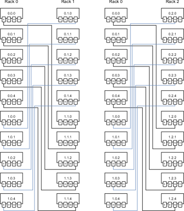
Figure 4: Illustration of the example diagrams created from the output of our scripts, facilitating the cabling process. The diagrams show all the inter-rack connections and the corresponding ports in switches. Each switch is labeled using a triple $(S,R,I)$, where $S\in\{0,1\}$ indicates the subgroup type, $R\in\{0,...,4\}$ indicates the rack, and $I\in\{0,...,4\}$ is the consecutive switch ID within a rack/subgroup. Then, we only show ports 8–11; these ports are used to connect racks. Ports 1–4 (for endpoints) and 5–7 (for intra-rack switch-switch links) are omitted for clarity.

3.4 Correctness Verification

We provide a set of scripts that ensure the correctness of the cabling. These scripts utilize the auto-generated port-to-port link descriptions and rack placements for each switch and compare it with the output of ibnetdiscover, an IB command that performs fabric discovery. This allows us to not only identify incorrectly wired cables and provide concrete instructions on how to rectify mistakes, but also detect missing or broken links. These scripts could even be used on a live cluster, while going through the wiring process, to immediately identify and flag errors.

4 HIGH-PERFORMANCE MULTIPATHING

We now propose a novel high-performance multipath routing protocol for low-diameter networks, which we use on the described SF deployment. For this, we extend the recently proposed FatPaths multipath routing protocol so that it offers vastly superior throughput while still ensuring very low latency.

Figure 5: Layered routing in FatPaths and in this work. Traffic is divided and sent using different layers. Our scheme relaxes the requirement in FatPaths for all layers to be trees. This ensures more flexibility in developing layers, leading to more throughput. Specifically, while in FatPaths, paths in different layers often overlap (cf. Layer 1 and 2), our routing alleviates this issue and reduces overlap/congestion and increases performance.

4.1 Original FatPaths Routing in Slim Fly

In terms of path diversity, FT has multiple same-length minimal paths between any two edge switches. Thus, one often uses ECMP [27] for multipath routing in FT. In SF (and to some degree in DF [28]), there is usually only one minimal path, but multiple “almost” minimal paths between any switch pair. This makes it challenging to achieve high path diversity in SF using ECMP. To alleviate this and to enable non-minimal high-speed multipathing in SF, the FatPaths architecture has recently been proposed [28]. FatPaths harnesses the concept of layered routing [29, 30] for low-diameter networks. In layered routing, one first creates layers: subsets of switch-switch links. Within one layer, one uses shortest-path routing. However, as a layer does not contain all the links, paths within this layer are usually non-minimal (in the global sense). If two nodes want to communicate using multiple paths, the sending node simply sends its data using paths residing in different layers. Note that multipathing is orthogonal to transport-level issues, and one can use different layers to transfer different flows between two nodes, but also different packets or flowlets within one flow [28]. In FatPaths, selecting links (when constructing layers) is done with simple random uniform sampling; a more elaborate scheme minimizing load imbalance is also provided. Layered routing is summarized in Fig. 5.

4.2 Proposed Multipath Routing: Summary

The central issue in layered routing is how to divide links into layers. We aim to minimize the number of layers (which minimizes the usage of HW resources in switches) while simultaneously maximizing the number of disjoint and almost-minimal paths between any switch pair (for more path diversity). Moreover, a detailed analysis from FatPaths indicates that – to maintain high performance in layered routing in virtually all low-diameter networks and traffic patterns – at least three disjoint paths per switch pair are needed [28]. Thus, the main goal of the layer construction algorithm is to find a minimum set of layers that together provide each switch pair with at least three disjoint paths while ensuring minimum overlap between specific layers. Ideally, these three paths include the minimal one (that always exists) and two “almost” minimal ones (in the following, an “almost” minimal path means a path that is longer by one hop than the minimal path between two given switches).

An overview of our proposed layer routing is shown in Fig. 5 (right). The key difference between our scheme and FatPaths is that we do not remove links from layers in order to ensure deadlock-freedom or to introduce non-minimal paths. Instead, we explicitly construct paths satisfying the appropriate constraints on their count, non-minimal length, and well-balancedness. This facilitates creating layers that result in much higher throughput.

4.3 Generating Routing Layers

Our layer construction scheme is detailed in Algorithm 1. The input is the topology of inter-switch connections $G=(V,E)$, and the desired number of layers $|L|$. The output is a set of layers $L$, where each layer contains a collection of paths connecting different pairs of nodes. These paths together define a separate forwarding tree for each node.

The layer generation starts with assigning all links to layer 1. In layer $1$, we only use minimal paths, as we want to ensure that the single minimal path existing between all node pairs is included in at least one layer for each pair. Moreover, a matrix $W$ and a priority queue $p$ are initialized. These structures are used to find advantageous non-minimal paths for each node pair. Intuitively, a priority $p(u,v)$ of a node pair $u,v$ is determined by the number of non-minimal paths already assigned to $u,v$ (and maintained in other layers). The higher $p(u,v)$ is, the lower the priority of $u,v$ is. Hence, when looking for new non-minimal paths, node pairs with fewer paths assigned are prioritized. This facilitates balancing the number of advantageous paths across all pairs of nodes, to eliminate potential hotspots in the network.

Second, each entry $W(r,s)$ in matrix $W$ describes the weight of a link between switches $r,s$. This weight equals the number of paths (from any layer) that already use this link. The higher $W(r,s)$ is, the more paths use the corresponding link. Hence, when selecting new paths, we use $W$ to balance numbers of paths across single links, minimizing risk of congestion. We also use $W$ to balance the paths in the first layer to ensure minimal overlap of minimal paths.

Then, for every layer $2\dots|L|$, and for each node pair in each layer, we find a single almost-minimal path that minimizes overlap with respect to paths already added to any other layer. For this, when finding paths in a layer $l$, we first copy the current priorities of node pairs into a list that preserves the current state of priorities (copy_pairs). Here, node pairs with the same priority are in a random order, but come before any node pair with lower priority. Note that each node pair appears twice in the list, once for each direction. This enables using different paths when routing in different directions, further increasing the flexibility of path selection.

After that, we iterate over each node pair, in an attempt to construct a path for each such pair in each layer. Note that, in principle, it is possible that one cannot find a path for each node pair in each layer (we elaborate on dealing with such rare cases in § B.1; we resolve them with a simple fallback to a minimal path – our evaluation shows that this does not negatively impact throughput).

In each such iteration, we first use the find_path routine to try to find an almost-minimal path for a given node pair $pair$, based on already inserted paths for that layer (specified in $l$) and weights assigned to each link (specified in $W$). If we are able to find a valid path, we accordingly update priorities $p$ (update_priorities) and link weights $W$ (update_weights). Finally, we insert the path into layer $l$ (add_path_to_layer).

Input :  Network topology $G=(V,E)$, number of layers $|L|$

Result :  A set of $L$ routing layers

 // $W\in\mathbb{R}^{N_{r}\times N_{r}}$ contains weights of links; $p$ is a priority queue, with entries being pairs of nodes

$W$ = init_link_weight_matrix()

 // Set all matrix entries to 0

$p$ = init_p_queue($G$)

 // Each node pair gets the same priority

$L$ = $\{E\}$

 // Layer 0 contains all the links ($E$)

1 for $l=1$ to $|L|-1$ do

       init_layer($l$)

       // Initialize the next layer as empty

2       $node\_pairs$ = copy_pairs($p$)

3       while $node\_pairs\neq\emptyset$ do

4             $pair$ = $node\_pairs$.dequeue()

5             $path$ = find_path($G$, $W$, $pair$, $l$)

6             if valid($path$) then

7                   update_priorities($path$, $p$)

8                   update_weights($path$, $W$)

9                   add_path_to_layer($path$, $G$, $l$)

10                  

11             end if

12            

13       end while

      $L=L\cup\{l\}$

       // Add a new layer to finalized layers

14      

15 end for

16

Algorithm 1 Construct routing layers; details are in § 4.3

5 IMPLEMENTATION OF MULTIPATHING

The IB architecture [5] enables a high-speed switched fabric with HW support for RDMA [6, 31] and atomic operations [32]. IB provides lossless destination-based packet forwarding that relies on link-level, credit-based flow control [33]. We now discuss the used IB features.

An IB network usually forms a single subnet consisting of physical IB switches and Host Channel Adapters (HCAs) that correspond to Ethernet NICs. All communication up to and including the transport layer is implemented within these two components.

Routing configuration is managed by a centralized subnet manager (SM). The SM configures connected IB devices, appropriately computes the forwarding tables to implement the used destination-based routing algorithm, and monitors the network for failures. Within an IB subnet, each HCA and each switch receive a unique local identifier (LID), assigned by the SM.

Each physical IB port has several independent virtual lanes (VLs). Each VL has its own receive and transmit buffers and flow control resources. There can be up to 15 VLs per physical port (depending on the equipment) and 1 VL for management traffic. Multiple VLs per port are used for deadlock freedom and to eliminate head-of-line blocking [33] (we discuss deadlocks in more detail in § 5.2).

Each switch provides a forwarding table called the Linear Forwarding Table (LFT) that – for a given packet – determines the outgoing port using the destination address (DLID) from the packet header. Then, for a given outgoing port, to determine the outgoing VL for a given packet, the switch uses a four-bit Service Level (SL) field from the packet header, in combination with the incoming and outgoing packet ports, to index into the SL-to-VL table. This enables packets to change virtual lanes at each hop and it allows for seamless utilization of switches with potentially different numbers of virtual lanes.

5.1 Routing

OpenSM, our choice of IB compliant SM, provides complete subnet information, including a list containing all nodes (switches, HCAs, routers) and ports, as well as the connections between them. We use this information to create and populate forwarding tables so that they implement the prescribed layered routing.

Multipathing In ECMP, each router stores multiple possible next-hops that each lie on a minimal path towards the destination. This approach of storing multiple next-hops for a given destination is not possible in IB. However, it can be emulated by assigning multiple LIDs to each HCA, a feature that we use to enable multipathing and to implement our layered routing in an IB setting. An HCA can receive a contiguous range of LID addresses. This range is determined by the so called LID Mask Control (LMC) value. Specifically, for an LMC equal $x$, each HCA port hosts a consecutive range of $2^{x}$ LIDs. Then, one routes towards each such LID using a different path. We use the information provided by OpenSM to appropriately populate forwarding tables so that they implement the layered routing described in § 4.

Implementation of Layers We assign multiple addresses to each node; one address falls into one layer (each layer gets one address from each node). Hence, a layer is physically formed by the assigned addresses and the associated forwarding entries that route traffic to these addresses. The forwarding entries are set according to the specification of layers in the initialization phase. Our scheme for constructing layers provides a data structure $port$, which specifies the output port to be used for a packet traveling to a node $d$, from a switch $s$, within a layer $l$; this output port is denoted with $port[l][s][d]$.

Routing Within Layers The number of layers equals the number of addresses assigned to each node. Thus, we can treat the layer ID as the offset to the base (i.e., to the first) LID of each node. Hence, for instance, routing in the first layer (ID $0$) uses the base LID of each node, whereas routing in the second layer uses the base LID plus offset 1.

Populating Forwarding Tables To populate forwarding entries, we add a value $port[l][s][d]$ into the LFT of switch $s$, as the outgoing port number for packets being routed towards node $d$. As the destination address, we use the base LID of the node, increased by the offset $l$, to ensure routing within layer $l$. As the last step, we run a deadlock-resolution scheme that fills all SL-to-VL tables, eliminating the risk of deadlocks (cf. § 5.2).

5.2 Deadlock-Freedom

One downside of IB’s credit-based flow control ensuring losslessness is the possibility of deadlocks. Specifically, an IB network may enter a state in which packets in different buffers wait for each other indefinitely long to free the buffers, resulting in a deadlock. To overcome this, most routing schemes use different VLs to send packets [34, 35, 36, 37, 38, 39]. By splitting a single port buffer into multiple independent logical VLs, one can break dependencies between waiting packets.

In FatPaths, each layer is acyclic, to ensure no deadlocks within each layer. However, this does not imply global deadlock-freedom on IB because of its lossless design based on channels. Specifically, one has to ensure that dependencies between packets using routes stored in any layers are also deadlock-free. Thus, we change the FatPaths approach by decoupling deadlock-avoidance from layer creation. Instead, we apply deadlock-removal after the layers are created. This also enables much more throughput because acyclic layers vastly restrict the choice of paths to be taken.

In our IB implementation, we propose and enable the use of two different deadlock-avoidance schemes. Firstly, if a sufficient number of VLs is available, we use the scheme introduced with the Deadlock-Free Single Source Shortest-Path (DFSSSP) [35] algorithm, which is already integrated in IB. Intuitively, given a ready routing (i.e., the populated forwarding tables), DFSSSP first finds all dependencies that could lead to a deadlock, and then it iteratively accommodates these dependencies in a deadlock-free way, by assigning selected routes to use yet unoccupied VLs. If not enough VLs are available, the algorithm fails. If not all VLs are exhausted, DFSSSP additionally balances the number of paths using each VL, for more throughput.

By increasing the number of layers used, the total number of unique paths between node pairs increases, resulting in a higher number of virtual lanes (VLs) required to resolve deadlocks using the DFSSSP scheme. To maximize the number of supported layers, we propose a novel deadlock avoidance scheme based on the Duato’s approach [40], that is agnostic to the number of layers and tailored for IB deployments that rely exclusively on paths of length $<=3$, such as those based on SF with our multipath routing method. The proposed algorithm ensures that the first, second, and third inter-switch hop of any path connecting two nodes use disjoint subsets of VLs. To achieve this, at least three VLs need to be available, and switches, for a given packet, must be able to identify their respective positions on the path using only the packet’s SL, incoming and outgoing port.

To illustrate the algorithm’s functionality, we consider each case individually. The first case, which involves paths of length 1 ($sw_{1}-sw_{2}$), can be solved trivially since $sw_{1}$ can determine that it is the first hop along the path by checking whether the incoming packet port is connected to an endpoint. This information can then be encoded easily in the SL-to-VL table.

To address the second case, paths of length 2 ($sw_{1}-sw_{2}-sw_{3}$), we adopt the same approach as used in case three. In the third and final case, paths of length 3 ($sw_{1}-sw_{2}-sw_{3}-sw_{4}$), we treat $sw_{1}$ as in case one, but we use a different approach to differentiate between $sw_{2}$ and $sw_{3}$. We establish a proper coloring of switches using all available SLs, resulting in each switch being assigned a unique SL among its neighbours. By setting the SL of any packet routed along a path of length 2 or 3 to the SL assigned to the second switch ($sw_{2}$) along that path, we can differentiate the second hop from a potential third hop and select the appropriate subset of VLs at each hop accordingly.

If fewer than $3$ VLs are available or no proper coloring using the available SLs can be established, the algorithm fails. Similar to the DFSSSP scheme, the disjoint VL subsets can be chosen to balance the number of paths crossing each VL.

5.3 Load Balancing

For load balancing, we rely on the respective protocol higher up in the stack to choose a layer out of the set of possible ones available for a given destination. In our case, this is the Open MPI [41] implementation of the Message Passing Interface (MPI) standard [42]. Open MPI serves as a communication library and directly interfaces with the IB networking API (Verbs). To optimize traffic flow, we utilize Open MPI’s default load balancing technique, which distributes traffic evenly across the available paths using a round-robin selection process. More advanced, adaptive schemes can seamlessly be used by changing the selection policy.

For fault tolerance, we rely on IB’s subnet manager. We stress that our routing can be seamlessly used with other transport schemes besides the ones used in the deployed cluster.

5.4 Path Diversity vs. Network Size

Increasing the number of different paths between each node pair requires more layers and thus also more addresses assigned to each node (i.e., a larger LMC value). However, using more addresses within one node decreases the maximum number of nodes that can be used in the network overall (because the address field size is fixed to 16 bits). We analyze this tradeoff in Tab. 2. We assume the maximum SF network based on {36, 48, 64}-port switches, that guarantees full global bandwidth. The results illustrate that one can use $4$ layers without having to make any compromises on the networks size, but anything beyond $4$ layers would reduce the maximum network size. At this point, the constraining factor is no longer the switch radix, but the address space. In § 6 and § 7, we show that – fortunately – our routing scheme’s performance is already quite substantial with just 4 layers and does not need more than 8 layers for high performance.

Table 2: Maximum number of switches and servers supported by a single-subnet, full global bandwidth, SF-based IB network, with $2^{LMC}$ many addresses per switch. “L”: LMC, “#A”: Number of addresses per server.

		36-port switches				48-port switches				64-port switches
L	#A	$N_{r}$	$N$	$k^{\prime}$	$p$	$N_{r}$	$N$	$k^{\prime}$	$p$	$N_{r}$	$N$	$k^{\prime}$	$p$
0	1	512	6144	24	12	882	14112	31	16	1568	32928	42	21
1	2	512	6144	24	12	882	14112	31	16	1250	23750	37	19
2	4	512	6144	24	12	800	12000	30	15	800	12000	30	15
3	8	450	5400	23	12	450	5400	23	12	450	5400	23	12
4	16	288	2592	18	9	288	2592	18	9	288	2592	18	9
5	32	162	1134	13	7	162	1134	13	7	162	1134	13	7
6	64	98	588	11	6	98	588	11	6	98	588	11	6
7	128	72	360	9	5	72	360	9	5	72	360	9	5

Figure 6: Histograms of average path lengths and maximum path lengths across all layers for each switch pair.

Figure 7: Histograms (bin size = 20) of counts of paths crossing each individual link.

Figure 8: Histograms of counts of disjoint paths for different switch pairs.

Figure 9: Maximum achievable throughput for the adversarial traffic pattern under three different injection loads (fraction of communicating endpoint pairs).

6 THEORETICAL ANALYSIS

We conduct a theoretical analysis of the developed routing protocols using the deployed SF network as a case study. We focus on how well our routing uses the diversity of non-minimal paths, which is necessary for high performance [28].

Baselines and Parameters

We analyze our layered routing that minimizes path overlap ( § 4) and compare it to a simple random layer construction (RUES, Random Uniform Edge Selection) and to the state-of-the-art FatPaths scheme [28].

We vary different parameters, including the fraction $p$ of preserved links in a layer, which refers to the proportion of links from the network that are included in each layer for the RUES scheme (specifically, we consider $p=40\%$, $p=60\%$, and $p=80\%$), and the number of layers used. Higher values of preserved links result in denser layers, making maximal and average path lengths lower. We focus on the deployed SF with 50 switches, but the results generalize to larger sizes. Overall, we show that the proposed layered routing is superior to the state-of-the-art in crucial metrics: lengths, distribution, and diversity of used paths, and the achieved throughput.

6.1 Path Lengths

The first important metric for evaluating routing is the length of paths constructed using the proposed routing schemes. Specifically, when routing in SF, one wants to use the single available minimal path (with 1 or 2 hops, depending on picked switch pairs) and the “almost” minimal ones – with 3 hops – as indicated in the FatPaths study [28]. To analyze whether the considered routing ensures this, we compute the average and maximum lengths of the set of paths connecting each individual switch pair, as produced by the respective routing schemes. Fig. 6 shows the analysis results.

Our novel layered scheme outperforms all others, because it ensures that the highest fraction of switch pairs uses the “almost” minimal paths of length at most 3. The downside of RUES is that the more randomness is employed, the larger the maximum path length becomes. For a sampling factor $p=80\%$, there is no switch pair with a path of length more than $4$, whereas for $p=40\%$ some switch pairs have paths of length greater than $8$. This indicates large differences in path lengths in different layers for some switch pairs, even if the average path length is between $3$ and $4$. This can negatively impact load balancing efforts as it becomes more difficult to predict path latency. Then, in FatPaths, large fractions of switch pairs use paths of length 2, which means that these links may likely become congested.

Doubling the number of layers does not change the overall trends and it has mostly no effect on the average path length distributions. Only the maximum path lengths display a small shift to the right. This is because using more layers increases the probability of finding a longer path.

6.2 Path Distribution

We now count the total number of paths that cross each individual link, see Fig. 7. Our layered routing ensures a balanced scenario, i.e., close to equal utilization of each link. This corresponds to a “single bar”, i.e., the “tighter” the distribution the better balanced the paths are.

Similarly to the analysis on path length, less randomness leads to better results, which is expected because as layers become less dense, the links that are present will be more utilized. Hence, any link that by chance is included in more than an average number of layers will have a higher number of crossing paths and vice versa. FatPaths performs similarly to RUES for a sampling factor of $p=80\%$. The distributions for $8$ layers are slightly shifted to the right compared to 4 layers, as they have twice as many paths.

6.3 Path Diversity

Two paths are disjoint if they do not share common links. In layered routing, we aim to maximize the number of such paths used by node pairs. Fig. 8 displays counts of disjoint paths between switch pairs. The FatPaths layer construction based on minimizing path overlap underperforms because of its acyclic layers. Moreover, unlike in previous analyses, more randomness (and thus sparser layers) leads to better result for RUES. For a sampling factor of $p=40\%$ and $8$ layers, $\approx$97.5% of switch pairs have at least the $3$ desired disjoint paths. This is the best performing algorithm out of the ones considered. However, this comes at the expense of disadvantageous path lengths and path distribution.

Our scheme does not need to make a similar trade-off because with $8$ layers already around $88.5\%$ of switch pairs have at least $3$ disjoint paths, which we have verified to grow to almost $100\%$ percent when scaling to the next higher configuration that uses $16$ layers. At the same time, the lengths and path distributions over links are highly beneficial.

6.4 Maximum Achievable Throughput

We also analyze the maximum achievable throughout (MAT). MAT is defined as the maximum fraction of traffic demands from all endpoint pairs that can be accommodated simultaneously, while adhering to network and routing constraints. For example, a throughput of $1.5$ denotes that the network can sustain $1.5$ times the traffic demand of each communicating node pair simultaneously.

Here, we consider an adversarial traffic pattern, which maximizes stress on the interconnect by incorporating several large elephant flows between endpoints that are separated by more than one inter-switch hop, and combining these large flows with many small flows [43]. We use TopoBench [43], a throughput evaluation tool which relies on linear programming to compute MAT. The results are displayed in Fig. 9.

Our algorithm outperforms FatPaths for different traffic intensities and layer counts. This is the most important for a small number of layers, which is key for routing on IB hardware as using many layers decreases the supported network sizes (cf. Tab. 2). Our layered routing experiences diminishing returns beyond 16 layers. This is expected, because almost $100\%$ of endpoint pairs have at least $3$ disjoint paths for $16$ layers (one needs at least that many disjoint paths to ensure high performance with non-minimal routing). Before diminishing returns set in, FatPaths requires $8\times$ as many layers to reach equivalent performance, making our design much more practical.

6.5 Insights & Takeaways - Theoretical Results

Our novel IB layered routing achieves superior performance in all considered path quality measures and especially in MAT. Almost around $60\%$ of switch pairs have at least $3$ disjoint non-minimal paths when using only $4$ layers, which grows to $88.5\%$ with $8$ layers. Furthermore, we achieve the most balanced distribution of paths over the links in the network. FatPaths performs similarly in terms of average and maximum path lengths, but underperforms in the available number of disjoint paths per switch pair. For RUES, a sampling factor of $p=60\%$ achieved the most balanced results across all metrics, but RUES performs much worse in comparison to FatPaths and our work overall.

Table 3: Workload Configurations.

Workload	Configuration	# Nodes	Scaling	Metric
Custom Alltoall	Message Sizes: $1$B $\to$ $4$MiB	$2,4,8,16,32,64,128,200$	Weak	Bandwidth [MiB/s]
IMB Bcast/Allreduce [44]	Message Sizes: $1$B $\to$ $32$MiB	$2,4,8,16,32,64,128,200$	Weak	Bandwidth [MiB/s]
eBB [45]	Message Size: $128$MiB	$2,4,8,16,32,64,128,200$	Strong	Bandwidth [MiB/s]
CoMD [46]	$100^{3}$ Atoms per Process	$25,50,100,200$	Weak	Time [s]
FFVC [47]	$128^{3}$ Cuboid per Process for $\leq 64$ processes, else $64^{3}$	$25,50,100,200$	Weak	Time [s]
mVMC [48]	Unmodified job_middle weak-scaling test	$25,50,100,200$	Weak	Time [s]
MILC [49, 50]	benchmark_n8 Input	$25,50,100,200$	Weak	Time [s]
NTChem [51]	taxol Model	$25,50,100,200$	Strong	Time [s]
BFS16 [52, 53]	# Vertices: $2^{23}$, $2^{24}$, $2^{25}$, $2^{26}$ Avg. Degree: $16$	$25,50,100,200$	Weak	Giga-Traversed Edges per Second [GTEPS]
BFS128 [52, 53]	# Vertices: $2^{23}$, $2^{24}$, $2^{25}$, $2^{26}$ Avg. Degree: $128$	$25,50,100,200$	Weak	Giga-Traversed Edges per Second [GTEPS]
BFS1024 [52, 53]	# Vertices: $2^{23}$, $2^{24}$, $2^{25}$, $2^{26}$ Avg. Degree: $1024$	$25,50,100,200$	Weak	Giga-Traversed Edges per Second [GTEPS]
HPL [54]	Matrix $A$ $\approx 1\text{ GiB },1\text{ GiB },1\text{ GiB }\text{ and }0.25\text{ GiB }$ pre Process	$25,50,100,200$	Weak	Giga-Floating point OP/s [GFLOPS]
ResNet152 [55, 56]	Pure Data Parallelism	$40,80,120,160,200$	Weak	Iteration Time [s]
Cosmoflow [56, 57]	Model Shards: $4$ Data Shards: $\frac{\text{\# Nodes}}{4}$	$40,80,120,160,200$	Weak	Iteration Time [s]
GPT-3 [58, 56]	Pipeline Stages (layers): $10$ Model Shards: $4$ Data Shards: $\frac{\text{\# Nodes}}{40}$	$40,80,120,160,200$	Weak	Iteration Time [s]

(a) MPI Bcast - SF L vs. FT

(b) MPI Allreduce - SF L vs. FT

(c) Custom Alltoall - SF L vs. FT

(d) eBB - SF L vs. FT

Figure 10: Relative performance difference of SF (linear placement strategy) over FT for various Microbenchmarks; eBB performance of SF L in comparison to maximum bandwidth and FT performance (higher is better), including routing improvement of this work over DFSSSP. Bidirectional bandwidth measured to be $5870\pm 10MiB/s$ using the ib_*_bw tools from the OFED perftest package [59].

Figure 11: Runtime of scientific workloads (lower is better) - SF L vs. FT

Figure 12: Performance of HPC benchmarks (higher is better) - SF L vs. FT

Figure 13: Iteration time of DNN proxy workloads (lower is better) SF L vs. FT and routing improvement of this work over DFSSSP for SF L.

7 EVALUATION

We now illustrate the feasibility of our SF installation by evaluating a broad set of applications from numerous domains against a comparable FT installation.

7.1 2-Level Non-Blocking Fat-Tree

FT topologies have historically been the prevalent choice for large-scale computing systems, largely due to their predictable behavior and full-bandwidth capabilities, when configured in a non-blocking manner. However, their high cost often leads to oversubscribed deployments at the tree’s lowest level, reducing construction costs at the expense of bisection bandwidth.

To ensure a fair performance comparison with our SF installation, we construct a 2-level non-blocking FT, reusing the same hardware. The FT and SF both share the same network diameter and full-bandwidth capabilities. Our FT configuration employs 6 core and 12 leaf switches, compatible with our 36-port switches. Each leaf switch connects to each core switch through 3 links, and the remaining ports link to evenly distributed endpoints. This configuration supports up to 216 endpoints, making the FT marginally under-subscribed and thus strengthening the fairness of our comparison.

7.2 Workloads & Configurations

We utilize a significant subset of the benchmarks included in the TSUBAME2 HyperX (t2hx) benchmark suite [10] and enhance them with a custom implementation of MPI_Alltoall, as well as three DNN proxies introduced by Hoefler et al. [56]. The configuration of each benchmark is provided in Tab. 3. Our analysis includes three classes of benchmarks:

Microbenchmarks We evaluate the system’s bandwidth using Intel MPI Benchmarks’ (IMB) measurements of the Allreduce and Bcast collectives [44], and a custom alltoall. We also assess the effective bisection bandwidth (ebb) of the system using Netgauge’s eBB benchmark [45].

Scientific Application & HPC Benchmarks We evaluate a wide range of benchmarks that cover various scientific applications, all of which are listed in Tab. 3 and taken directly from the t2hx benchmark suite. We also analyze the performance of the High Performance Linpack (HPL) [54] benchmark and the breadth-first search (BFS) [60] performance in the Graph 500 Benchmark [52]. Additionally, we extend the BFS performance analysis by changing the average degree of the vertices (edgefactor), while scaling the number of vertices linearly with the number of participating compute nodes. Specifically, we consider edgefactors $16$, $128$ and $1024$.

DNN Proxies The DNN proxies evaluated on SF include ResNet152 [55] (pure data parallelism), CosmoFlow [57] (data and operator parallelism) and GPT-3 [58] (data, operator, and pipeline parallelism), as outlined in Tab. 3. For GPT-3, each pipeline stage processes one DNN-layer.

7.3 Execution Environment

To ensure consistency and reproducibility, all benchmarks were compiled using GCC v4.8.5 and executed using OpenMPI v1.10.7. We use one MPI rank per node and assign one OpenMP thread per physical core on Socket 1 of the dual-socket system (pinning on Socket 2 introduces non-negligible slowdowns due to inter-socket communication).

We investigate two MPI rank placement strategies: linear and random. The linear strategy places rank $j$ on node $j$, a commonly used approach that enhances latency and traffic locality, especially for FTs  [61, 62]. This strategy also models a system with minimal fragmentation. In contrast, the random strategy represents systems with significant fragmentation. It randomizes rank placement to potentially reduce network bottlenecks on SF, albeit at the cost of increased latency. For FT, the linear placement significantly outperformed its random counterpart in all microbenchmarks and exhibited comparable performance in the remaining tests. Consequently, we report SF performance relative to the FT’s linear placement only.

Each benchmark configuration is executed five times; microbenchmarks are executed for at least 100 iterations. We assess all SF benchmarks using our new multipath routing algorithm based on both minimal and almost minimal paths, as well as the defacto standard multipath routing algorithm in IB (DFSSSP), that leverages minimal paths only [63]. We instantiate each routing algorithm once with 1, 2, 4, and 8 layers, respectively, but only report the results of the best-performing variant for each benchmark configuration. For all FT benchmarks we choose the commonly used ftree routing [64]. Mean and standard deviation of the results are reported, with the latter indicated using red error bars for all bar plots. Relative performance differences of SF over FT are annotated above each bar. Any significant performance gains or losses of our novel routing algorithm in comparison to DFSSSP for any benchmark are either explicitly stated in the text or visualized using heatmaps.

For space considerations, we report only the linear placement strategy for SF in the main text. Results for the random placement strategy are available in appendix C.

7.4 Microbenchmarks

Fig. 10(a)–10(c) illustrate the relative performance differences of SF (with linear placement) over FT for MPI collectives bcast, allreduce, and custom alltoall.

In general, SF’s performance is largely comparable to that of the FT. However, for 8 and 16-node configurations for bcast and allreduce – especially with smaller message sizes – the FT displays marginal advantages. This is can be attributed to FT having 16 nodes per switch rather than 4 as in SF, leading to more localized, zero inter-switch hop communication, which results in reduced latency.

In contrast, for the communication-intensive alltoall collective, SF’s performance closely mirrors, or even slightly surpasses, the FT for small message sizes. Yet, for bandwidth-critical message sizes in 8, 16, and 32 node configurations, SF lags. With the linear placement strategy in SF, all inter-switch communication for these configurations occurs between 2, 4, or 8 switches respectively, leading to traffic congestion on the often single shortest path between these switches. Although our new routing scheme should theoretically mitigate this, as shown in § 6, the system’s lack of adaptive load balancing limits its practical improvement to at most $7\%$ over DFSSSP. However, adopting the random placement strategy for SF, detailed in the appendix (see Fig.17(c) in appendix C), overcomes this bottleneck, slightly outperforming the FT. This suggests that combining adaptive load balancing with our new routing scheme could resolve the bottleneck even for the linear placement strategy.

Lastly, in Fig. 10(d), we present the ebb across various node counts. At maximum node count we achieve approximately half of the injection bandwidth, equating to $75\%$ of the theoretical bisection bandwidth optimum [1]. Though the FT matches SF’s full-system ebb, it outperforms SF for the 8, 16, and 32 nodes configurations. This discrepancy mirrors the observations for the alltoall collective and shows similar behavior with the random placement strategy, as depicted in Fig.17(d) in the appendix.

In the right section of Fig. 10(d), a heatmap displays the performance gains of our new routing scheme over DFSSSP for the eBB benchmark. Notably, we see improvements of up to $28\%$ for the earlier described node configurations, which are especially prone to congestion on the shortest paths.

7.5 Scientific Workloads & HPC Benchmarks

In Fig. 11, we present the runtime and relative performance of the solver/kernel for each of the scientific workloads on SF, using the linear placement strategy. The scaling behavior of each workload, based on their configurations detailed in Tab. 3, is evident. Notably, the drop in runtime for FFVC when scaling from 50 to 100 nodes is due to the decrease in the workload’s problem size when running on $>64$ nodes. Utilizing almost minimal paths in combination with minimal paths does not generate any significant speedup for these workloads over pure minimal routing (DFSSSP), and generally results in only small runtime variances of $<1\%$. This is due to the communication time only constituting a small fraction of the overall runtime for these scientific workloads [10, 65].

Fig. 12 shows the performance of the HPC benchmarks, which display similar weak-scaling behavior as the scientific workloads. HPL exhibits almost linear scaling performance when increasing the number of nodes from $25$ to $50$ or $100$ nodes, indicating that the overhead introduced by the increased amount of communication is negligible. Consistent with these results, introducing almost minimal paths to the routing impacts performance by less than $1\%$ for the HPL benchmark. The only exception is the $200$ node setting, where the decrease in the problem size (per node) is likely the main cause for the deviation from the linear scaling observed.

In the case of the Graph 500 - BFS benchmark, we experienced high variance with the default implementation. To mitigate this, we fixed the seed for the graph generation and used the same source vertex for each BFS run. The BFS scaling results show more fluctuations in comparison to the HPL results, particularly for the sparser variant. This is accompanied by greater variability in speedup through almost minimal paths, which ranged from -$5\%$ to +$1\%$. It is not clear whether this can be attributed purely to network communication or to other factors such as caching effects and system noise.

Overall, our experiments show SF competes effectively with FT in terms of performance, while being very effective for scaling both scientific workloads and HPC benchmarks, even when limited to minimal paths.

7.6 Deep Learning Workloads

The left part of Fig. 13 shows the runtime and relative performance of the DNN proxies when linearly increasing the number of nodes from $40$ to $200$. ResNet152 with pure data parallelism only requires allreduce for gradient aggregation. CosmoFlow with a hybrid of data and operator parallelism requires allgather, reduce-scatter, allreduce, and point-to-point communications. GPT-3 with a hybrid of data, operator, and pipeline parallelism requires allreduce and point-to-point communications. As we increase the data shards proportionally to the number of nodes, the scalability is mainly determined by allreduce across the data dimension.

We find that CosmoFlow’s runtime on SF is comparable to that on FT. In contrast, GPT-3 notably performs better on SF for configurations with 160 and 200 nodes, while ResNet152 begins to lag as the node count increases. Although both GPT-3 and ResNet152 predominantly rely on allreduces at higher node counts, their diverging performance trends can be attributed to differences in message sizes; GPT-3 handles significantly larger messages than ResNet152. Expectedly, the performance trend of GPT-3 matches the trend of MPI Allreduce for the high node count configurations (cf. Fig. 10(b)).

The right part of Fig. 13 shows that our work generally outperforms DFSSSP for GPT-3, with up to $24\%$ improvements.

7.7 Insights & Takeaways - Empirical Results

When analyzing communication-intensive workloads on configurations with 8, 16, or 32 nodes, we identified some congestion challenges. These challenges stemmed from the non-adaptive nature of the path selection. However, by employing a random placement strategy, these issues were effectively counteracted. Our findings subsequently indicate that SF consistently achieves performance on par with, or even surpassing, the well-established FT topology, particularly under conditions of full-system utilization. Additionally, SF displays effective scaling capabilities across a diverse range of workloads. In comparison to the established DFSSSP, our novel routing approach exhibited promising performance, registering improvements of over $20\%$.

7.8 Scalability & Cost Analysis

Table 4: Maximal scalability and costs of SF deployments compared to non-blocking FT2, FT2 oversubscribed by 3 (FT2-B), FT3 and 2-D HyperX (HX2) under given port constraints. For the fixed size cluster we use 64-port switches for the FT2 and FT-B, 40-port switch for HX2, and 36-port for SF and FT3.

	36-port switches					40-port switches					64-port switches					2048 nodes clusters
	FT2	FT2-B	FT3	HX2	SF	FT2	FT2-B	FT3	HX2	SF	FT2	FT2-B	FT3	HX2	SF	FT2	FT2-B	FT3	HX2	SF
Endpoints	648	972	11664	2028	6144	800	1200	16000	2744	7514	2048	3072	65536	10648	32928	2048	2048	2048	2197	2178
Switches	54	45	1620	169	512	60	50	2000	196	578	96	80	5120	484	1568	96	59	303	169	242
Links	648	324	23328	2028	6144	800	400	32000	2548	7225	2048	1024	131072	10164	32928	2048	344	4320	2028	2057
Costs [M$]	1.5	1.1	45	4.5	13.8	2.4	1.7	84.2	7.8	22.4	9	7.2	491	45.5	146	7.5	2.7	8.3	6.4	5.8
Cost/Endp [k$]	2.2	1.2	3.8	2.2	2.2	3	1.5	5.2	2.8	2.9	4.4	2.3	7.5	4.3	4.4	3.6	1.3	4	3.1	2.8

FT topologies are the preferred choice for large-scale HPC deployments due to their adaptability, adoptable bisection bandwidth, established routing, and isolation advantages. These properties often benefit application performance consistency  [66, 67, 68]. However, their low-diameter configurations do not scale as well as contemporary topologies [69].

We compare the scalability and deployment cost of 2-level FTs (FT2), 3-level FTs (FT3), 2-D HyperX (HX2) [10, 70], and SF. Our evaluation, summarized in Tab. 4, includes both the non-blocking FT2 variant and its 3:1 oversubscribed version (FT2-B). The pricing details are in appendix D.

Scalability

We show that SF networks offer a distinct advantage in scalability by evaluating maximum network size for a HW setup with 36, 40, and 64-port switches. SF can accommodate approximately 10, 6, and 3 times more endpoints than FT2, FT2-B, and HX2 respectively, while maintaining a lower or comparable cost-to-endpoint ratio and the same network diameter of 2. FT3 can accommodate more endpoints than SF, however, this comes at a significantly larger (around 1.75x) cost-to-endpoint ratio and increased network diameter which has an impact on a performance of latency critical applications. This makes SF a compelling choice for large-scale diameter-2 deployments.

Cost

When the number of endpoints is predetermined, SF’s requirement for fewer port switches can reduce overall deployment costs, while keeping comparable benchmark performance to FT2 as shown in § 7. Tab. 4 further shows an example of fixing a cluster requirement to 2048 endpoints. Realising such a cluster using SF in comparison to FT2, HX2, and FT3 results in absolute cost saving of $1.7M, $0.6M, and $2.5M respectively. While using FT2-B might be cheaper in this scenario, it does not provide the full bandwidth property as SF, FT2, HX2, and FT3.

8 RELATED WORK

Our work touches on different areas. We now outline related works, excluding the ones covered in past sections.

Network Topologies

Several recent networks build upon SF. This includes Megafly [71], Bundlefly [72], Galaxyfly [73], and Xpander [4]. Yet, they do not provide diameter-2 and thus none of them are competitive with SF in latency, cost, or power consumption, as observed by recent results [28]. Although PolarFly has shown promising results in recent studies, its advantages over SF can be attributed to the diligent design of routing protocols that leverage its structure to guarantee optimal routing decisions [74, 75]. Some recent designs based on similar principles target on-chip networks only [76, 77].

Physical Interconnect Installations

The majority of works on interconnects use simulations for evaluation [1, 2, 3, 4, 71, 72, 73, 78, 79, 80, 81]. However, some topologies have been evaluated with real installations. This includes – for example – HyperX [10] and Dragonfly [22]. Here, we offer the first real evaluation of Slim Fly.

Congestion Control & Load Balancing

In general, we do not focus on transport protocols (flow, congestion). Here, we rely on mechanisms from the FatPaths [28] architecture. In layered routing, traffic is balanced across layers. We use simple randomized and round-robin schemes, which results in high performance. Other schemes could also be incorporated, including load balancing based on flows [27, 82, 83, 84, 85, 86, 87, 88, 89], flowcells [90], flowlets [91, 92, 93, 94, 95], and single packets [96, 97, 98, 99, 100, 101].

9 CONCLUSION

Slim Fly (SF) is the first network topology that lowered cost and improved performance by reducing the network diameter to two, promising significant improvement over established interconnects. However, it has not yet been tested in practice. We address this by deploying the first at-scale SF installation and establishing and implementing open-source routines for cabling and physical layout, to guide future deployments and effectively verify cabling. This can foster the adoption of SFs in broad industry and facilitate practical deployments of other low-diameter topologies, including the most recent ones, such as PolarFly or Bundlefly.

We further introduce a novel high-performance routing scheme that improves upon state of the art, achieving up to $24\%$ speedup for the evaluated deep neural network (DNN) workloads over the standard IB multipath routing algorithm (DFSSSP) through non-minimal paths.

We use the first practical, real-world deployment of SF to demonstrate the topology’s ability to scalably process a wide selection of modern workloads such as distributed DNN training, graph analytics, or linear algebra kernels. It consistently matches or surpasses the performance of a comparable non-blocking Fat Tree (FT) deployment for a wide selection of workloads, for example, achieving a 66% speedup for distributed deep neural network training. Importantly, SF simultaneously delivers superior scalability. For example, it enables connecting between $3\times$ and $10\times$ the number of servers compared to other diameter-2 topologies like 2-level FT and 2-D HyperX, while maintaining both a comparable cost-to-endpoint ratio and full bandwidth. For larger installation sizes, SF’s scalability translates to significant cost advantages, for example, 50% over full bandwidth non-blocking 3-level Fat Tree configurations [1]. Overall, this effort will spearhead future research into more powerful network topologies.

Appendix A Details of Slim Fly Construction

A.1 Selecting Topology Size, Parametrizing Input

Overall, one first chooses a prime power $q$ that satisfies the equation $q=4w+\delta$ for some $\delta\in\{-1,0,1\}$ and $w\in\mathbb{N}$. $q$ is an input parameter that determines the whole topology structure. For example, the number of vertices (switches) is $N_{r}=2q^{2}$ and the network radix $k^{\prime}=\frac{3q-\delta}{2}$. In our case, $N_{r}=50$, thus $q=5$, which satisfies the equation $q=4w+\delta$ for $w=1$, $\delta=1$, and $k^{\prime}=7$. Hence, every switch is connected to $7$ other switches. Interestingly, this construction forms the famous Hoffman-Singleton graph [25, 26], which is optimal with respect to the Moore Bound. Finally, as a regular and direct network, it is recommended to attach $p=\left\lceil\frac{k^{\prime}}{2}\right\rceil$ endpoints to each switch to ensure full global bandwidth [1]. In our case, $p=4$.

A.2 Finding Needed Algebraic Structures

Once $q$ is selected, one uses it to construct several algebraic structures. Specifically, one finds a base ring $\mathbb{Z}_{q}$ (for us, $\mathbb{Z}_{5}=\{0,1,...,4\}$), its primitive element $\xi$ that generates all elements of $\mathbb{Z}_{q}$ (for us, $\xi=2$), and two generator sets $X=\{\xi^{0},\xi^{2},...,\xi^{q-3}\}$ and $X^{\prime}=\{\xi^{1},\xi^{3},...,\xi^{q-2}\}$ (for our installation, $X=\{1,4\}$ and $X^{\prime}=\{2,3\}$). While not complex, details on these structures are not necessary to understand our Slim Fly deployment. The interested readers may check them in the original publication [1].

A.3 Labeling and Connecting Switches

Each switch receives a 3-tuple label from a set $\{0,1\}\times\mathbb{Z}_{q}\times\mathbb{Z}_{q}$. Thus, SF switches come in two flavors determined by the first elements of their labels: $(0,\cdot,\cdot)$ and $(1,\cdot,\cdot)$. These labels determine how the switches are connected. Specifically, switches with labels $(0,\cdot,\cdot)$ are connected using the following equation [1]:

$$\text{switch }(0,x,y)\text{ is connected to }(0,x,y^{\prime})\iff y-y^{\prime}\in X.$$ (1)

Symmetrically, switches with labels $(1,\cdot,\cdot)$ use the following equation:

$$\text{switch }(1,m,c)\text{ is connected to }(1,m,c^{\prime})\iff c-c^{\prime}\in X^{\prime}.$$ (2)

Lastly, two switches with labels $(0,\cdot,\cdot)$ and $(1,\cdot,\cdot)$, respectively, are connected according to the following equation:

$$\text{switch }(0,x,y)\text{ is connected to }(1,m,c)\iff y=m\cdot x+c$$ (3)

A.4 Topology Structure & Physical Layout

The graph underlying the SF topology consists of two same-size subgraphs. One subgraph contains routers $(0,x,y)$, the other consists of routers $(1,m,c)$. Each subgraph contains $q$ identical groups of routers. Groups in different subgraphs usually differ from one another. There are no connections between groups within the same subgraph, i.e., no two routers $(0,x,y)$ from different groups are linked, the same holds for routers $(1,m,c)$. However, each group from one subgraph has connections to every other group in the other subgraph; thus the groups form a fully connected bipartite graph.

This property facilitates physical layout and we use it in our installation. Specifically, as recommended in the original work [1], we combine groups from different subgraphs pairwise; these combined groups form racks. In general, this leads to $q$ racks, each with $2q$ routers. In our installation, we have 5 racks, each with 10 routers and 40 compute nodes.

A.5 Constructing Slim Fly with N nodes

As the space of valid SF topologies is quite sparse, we show the simple steps needed to find a SF network with the number of nodes as close to N as possible:

1. Obtain the cube root R of the desired node count N

2. Find prime powers close to R

3. Obtain the corresponding full-bandwidth network configurations (see previous sections)

4. Verify network sizes and select the network that is closest to N in terms of number of supported nodes

Appendix B Routing Details

B.1 Details of Layer Generation

We provide more details on crucial parts of layer generation.

B.1.1 Finding Almost-Minimal Paths

We look for almost-minimal paths that are exactly 3 hops long (one hop longer than SF’s diameter of two), while balancing the number of paths crossing each link (to avoid highly congested links). We do not target longer paths, in order to conserve network resources (i.e., a flow taking fewer hops occupies fewer buffers).

For this, we design a heuristic based on a modified breadth first search graph traversal starting from the source node $src$, constraining the path length to 3. In theory one could also define a range of valid lengths. The heuristic obtains the set $P$ of all valid paths starting in $src$ and ending in the destination node $dst$; $P=\{(u_{1},\dots,u_{l})\mid l=3\wedge u_{1}=src\wedge u_{l}=dst\}$. Here, a path is considered valid if it satisfies the given length constraint $3$ and if its insertion into the layer does not affect any previously inserted paths. Then, we choose a path $p\in P$ that minimizes link weights, i.e., $\forall p^{\prime}\in P\ \omega(p)\leq\omega(p^{\prime})$ where $\omega(p)$ is the sum of weights of links included in $p$.

B.1.2 Node Pair Priority Queue

The order in which the paths are inserted is very important, because it may impact whether we are able to find new paths. If one would first find a given number of paths for a single node pair, and only then proceed to the next node pair, some node pairs might not receive any, or much fewer, paths than other pairs. To alleviate this, we balance the total number of added almost-minimal paths across all node pairs. For this, each node pair is assigned a priority value, equal to its total number of almost-minimal paths across all layers; the lower the value, the more important it is to find a path for this node pair. Therefore, the number of required priority levels is upper-bounded by $|L|-1$, because each node pair can have at most one almost-minimal path per each of $|L|-1$ layers, and is initially in the highest priority value (value of $0$). The lowest priority level is value $|L|-1$, which only contains node pairs who have had an almost-minimal path inserted in every layer.

Whenever a path is added to a layer, all of the node pairs that have a non-minimal path inserted have their priority decreased and they move up to the next higher priority layer. For instance, in Fig. 15 by assuming that the minimum length for an almost-minimal path is two, adding the illustrated path to a layer, results in both node pairs $(v_{1},v_{4})$ and $(v_{2},v_{4})$ having an almost-minimal path added for them (assuming we allow paths of length $2$ and $3$ as non-minimal paths and $dst$ is one of the receiving nodes). Therefore, both of their priorities would be decreased by $1$. This also assumes that the paths were not already in this layer, which could have been the case for $(v_{2},v_{4})$.

The $node\_pairs$ list generated from the priority queue $p$ in Algorithm 1 contains the entries of the priority queue in the order of priority value, and randomized within each level. Hence, the layer generation algorithm first tries to add an almost-minimal path for all nodes of priority value $0$ in a random order, and then move to the nodes of the next value. Hence, it first processes all node pairs with no inserted paths, then with one inserted path, and so forth, facilitating a balanced path distribution across node pairs.

B.1.3 Path Weighting

A weight update is performed after the insertion of a new path into any layer. The weight of each link in any existing path is increased by the total number of new “routes” that now occupy the link. An example is shown in Fig. 14. The weight of link $(v_{1},v_{2})$ is increased by $9$ because it has $9$ new routes using it, as there are $3$ sending nodes ($a_{1}-a_{3}$) and $3$ receiving nodes ($b_{1}-b_{3}$). The weight of link $(v_{3},v_{4})$ is increased by $27$ as there are $9$ sending nodes ($a_{1}-a_{9}$) and $3$ receiving nodes ($b_{1}-b_{3}$).

Figure 14: Illustration of the weight update methodology employed by the algorithm. After the insertion of the path from $v_{1}$ to $v_{4}$, the weights of the links $(v_{1},v_{2})$, $(v_{2},v_{3})$ and $(v_{3},v_{4})$ are increased by $9$, $18$, and $27$, respectively.

B.1.4 Potential Invalidity of Paths

For a given source $src$ and destination $dst$, it may happen that $P=\emptyset$, in which case no almost-minimal path is added to a given layer for that node pair. There are two scenarios when this may happen, we illustrate them in Fig. 15 and in Fig. 16. The first one occurs when a path for the node pair is already included in another (previously inserted) path into the layer. For instance, after the path in the figure is inserted into layer $l$, all sub-paths ($(v_{2},v_{4})$, $(v_{3},v_{4})$) become included as well, forcing $v_{2}$ and $v_{3}$ to route along minimal paths towards destination $v_{4}$ in layer $l$.

The second scenario occurs when no path of required length can be found because routing via any of the source node’s neighbors would result in a path too short or too long. In our second example, the almost-minimal paths are constrained to have length exactly $3$. At first, the two almost-minimal paths $q=(v_{1},v_{2},v_{3},u_{3})$ and $q^{\prime}=(w_{1},w_{2},w_{3},u_{3})$ are inserted, which fixes the paths for all node pairs in the set $\{(v_{i},u_{3}),(w_{i},u_{3})\mid i\in\{1,2,3\}\}$. Now any path for the node pair $(u_{1},u_{3})$ that respects the already inserted paths will have length $l\in\{1,2,4\}$ because it would have to come from the following set of paths: $\{(u_{1},q)$, $(u_{1},q^{\prime})$, $(u_{1},u_{3})$, $(u_{1},u_{2},u_{3})$, $(u_{1},u_{2},v_{2},v_{3},u_{3})$, $(u_{1},u_{2},w_{2},w_{3},u_{3})\}$. If this scenario occurs, we route minimally, i.e. path $(u_{1},u_{3})$.

Figure 15: Illustration of an almost-minimal path from $v_{1}$ to $v_{4}$, which enforces minimal routing from $src$ nodes like $a_{7}$, located on the sub-paths, to $dst$ nodes, i.e. $b_{1}$, in this layer.

Figure 16: Illustration of a scenario in which no almost-minimal, valid path of length exactly $3$ can be found for node pair $(u_{1},u_{3})$ in the given layer due to the prior insertion of two valid paths.

B.1.5 Specification of Forwarding Tables

In layered routing, each forwarding entry $(l,s,d)\in\text{layers}\times\text{switches}\times\text{switches}$ corresponds to the port that switch $s$ uses when routing in layer $l$ and transmitting a packet addressed to a switch $d$.

Appendix C Additional Results

C.1 Changes for Custom Alltoall

We decided not to use the OpenMPI’s default implementation of alltoall, as the algorithms it relies on result in sub-optimal performance for the deployed SF. Empirically, we determined that the best-performing alltoall for our system was a simple algorithm that posts all non-blocking send and receive requests simultaneously and then waits for completion. Other collectives did not show a similar impact, and we thus used the default implementations. These issues are not expected with newer hardware.

(a) MPI Bcast - SF R vs. FT

(b) MPI Allreduce - SF R vs. FT

(c) Custom Alltoall - SF R vs. FT

(d) eBB - SF R vs. FT

Figure 17: Relative performance difference of SF (random placement strategy) over FT for various Microbenchmarks; eBB performance of SF R in comparison to maximum bandwidth and FT performance (higher is better), including routing improvement of this work over DFSSSP. Bidirectional bandwidth measured to be $5870\pm 10MiB/s$ using the ib_*_bw tools from the OFED perftest package [59]

Figure 18: Runtime of scientific workloads (lower is better) - SF R vs. FT

(a) SF R vs. FT

(b) SF L vs. FT

Figure 19: Runtime of additional scientific workloads (lower is better)

Figure 20: Performance of HPC benchmarks (higher is better) - SF R vs. FT

Figure 21: Iteration time of DNN proxy workloads (lower is better) SF R vs. FT and routing improvement of this work over DFSSSP in SF R

C.2 Microbenchmarks

Fig. 17(a)–17(c) illustrate the relative performance differences of SF (with random placement) over FT for MPI collectives bcast, allreduce, and custom alltoall.

In general, SF’s performance is marginally worse than that of the FT for bcast and allreduce, especially for smaller node counts and message sizes. This is attributable to FT’s linear placement strategy and its leaf switches connecting to at least 16 nodes each, facilitating more localized communication with zero inter-switch hops, which results in reduced latency. Whereas in SF, messages need to traverse more inter-switch hops, especially due to the random placement strategy.

In contrast, SF significantly outperforms FT on the communication-intensive alltoall collective. Here the random placement strategy clearly demonstrates the trade-offs in terms of latency and traffic balancing for the SF topology. While this strategy does increase latency, particularly for smaller message sizes, it aids the routing in distributing traffic more uniformly across the network.

Lastly, we report in Fig. 17(d) the effective bisection bandwidth at different node counts. Importantly, the measured bandwidths on SF match the performance achieved on the FT and the random placement strategy helps to eliminate any congestion issues that were present with the linear placement strategy.

On the right part of Fig. 17(d), a heatmap illustrates the performance gains of our new routing algorithm over DFSSSP for the eBB benchmark. Unlike with the linear placement strategy, we only see marginal improvements of up to $7\%$.

C.3 Scientific Workloads & HPC Benchmarks

We show in Fig. 18 the runtime and relative performance of the solver/kernel for each of the scientific workloads on SF using the random placement strategy. We observe similar trends as for the linear placement strategy for all scientific workloads and SF’s performance aligns closely with FT’s, while no significant speedup or slowdown through the use of non-minimal paths could be observed.

In Fig.19, we present the relative performance of two additional scientific workloads, AMG[102] and MiniFE [103], on SF, using both placement strategies. For this assessment, AMG was configured with a $128^{3}$ cube per process, while MiniFE was set with grid input dimensions of $n_{{x|y|z}_{b}}=90$. In accordance with these configurations, clear weak-scaling behavior is evident under the random placement strategy. On the other hand, with the linear placement strategy, the observed trends are less distinct, and, there are instances where SF outperformed FT by unexpected margins. We believe that this disparity can’t be merely attributed to the variations in communication stemming from the placement strategy, as the applications in consideration aren’t generally communication-bound and the FT is fully non-blocking. However, the precise cause remains unclear.

Fig. 20 shows the performance of the HPC benchmarks on SF using the random placement strategy, results that largely mirror those obtained using the linear placement strategy.

C.4 Deep Learning Workloads

The left part of Fig. 21 shows the runtime and relative performance of the DNN proxies with the random placement strategy. The results are also very similar to those obtained using the linear placement strategy, including GPT-3 matching the performance trends of the MPI Allreduce pattern with the random placement strategy and comparable node counfigurations (cf. Fig. 17(b)).

However, similar to previous results, the right part of Fig. 21 shows that our work generally matches or outperforms DFSSSP, achieving up to a 1.18x speedup.

Appendix D Pricing details

We based our pricing on data colfaxdirect.com and SHI.com. Regarding the equipment selection, we use InfiniBand Topology Configurator . For different switch sizes, we selected different models from current Nvidia offerings. For example, for a 36-port switch, we chose Mellanox SB7800 EDR 100Gb/s. For a 40-port switch, we decided to use Mellanox Quantum QM8700 HDR 200Gb/s . Finally, for a 64-port switch, we use Nvidia QM9700 NDR 400G model. For AoC cables, we selected active fiber links, and for DAC cables, we chose passive copper cables for endpoint connections. Again, we base our estimations on mentioned earlier InfiniBand Topology Configurator online service. However, it can be challenging to determine the cost of networking hardware because the prices of such hardware can vary greatly depending on the quantity ordered, and large orders may be eligible for substantial discounts.

References

- [1] Maciej Besta and Torsten Hoefler “Slim fly: A cost effective low-diameter network topology” In ACM/IEEE Supercomputing, 2014, pp. 348–359 DOI: 10.1109/SC.2014.34
- [2] John Kim, Wiliam J. Dally, Steve Scott and Dennis Abts “Technology-Driven, Highly-Scalable Dragonfly Topology” In Proc. of Intl. Symp. Comp. Arch., ISCA ’08 Washington, DC, USA: IEEE Computer Society, 2008, pp. 77–88 DOI: 10.1109/ISCA.2008.19
- [3] John Kim, William J. Dally and Dennis Abts “Flattened Butterfly: A Cost-efficient Topology for High-radix Networks” In Proc. of Intl. Symp. Comp. Arch., ISCA ’07 San Diego, California, USA: ACM, 2007, pp. 126–137 DOI: 10.1145/1250662.1250679
- [4] Asaf Valadarsky, Michael Dinitz and Michael Schapira “Xpander: Unveiling the Secrets of High-Performance Datacenters” In ACM HotNets, 2015
- [5] The InfiniBand Trade Association “Infiniband Architecture Spec. Vol. 1, Rel. 1.2”, 2004 InfiniBand Trade Association
- [6] Robert Gerstenberger, Maciej Besta and Torsten Hoefler “Enabling highly-scalable remote memory access programming with mpi-3 one sided” In ACM/IEEE Supercomputing, 2013, pp. 1–12
- [7] Salvatore Di Girolamo et al. “Network-accelerated non-contiguous memory transfers” In ACM/IEEE Supercomputing, 2019
- [8] Jack J Dongarra, Hans W Meuer and Erich Strohmaier “TOP500 supercomputer sites” In Supercomputer 13 ASFRA BV, 1997, pp. 89–111
- [9] Maciej Besta et al. “High-Performance Routing With Multipathing and Path Diversity in Ethernet and HPC Networks” In IEEE TPDS, 2020
- [10] Jens Domke et al. “HyperX Topology: First At-Scale Implementation and Comparison to the Fat-Tree” In ACM/IEEE Supercomputing, 2019
- [11] Maciej Besta “To Push or To Pull: On Reducing Communication and Synchronization in Graph Computations” In ACM HPDC, 2017, pp. 93–104 ACM DOI: 10.1145/3078597.3078616
- [12] Maciej Besta et al. “Demystifying graph databases: Analysis and taxonomy of data organization, system designs, and graph queries” In ACM CSUR, 2023
- [13] Maciej Besta “SISA: Set-Centric Instruction Set Architecture for Graph Mining on Processing-in-Memory Systems” In ACM MICRO, 2021
- [14] Maciej Besta “GraphMineSuite: Enabling High-Performance and Programmable Graph Mining Algorithms with Set Algebra” In VLDB, 2021
- [15] Maciej Besta “High-performance parallel graph coloring with strong guarantees on work, depth, and quality” In ACM/IEEE Supercomputing, 2020
- [16] Maciej Besta “Practice of Streaming Processing of Dynamic Graphs: Concepts, Models, and Systems” In IEEE TPDS, 2022
- [17] Tal Ben-Nun et al. “A modular benchmarking infrastructure for high-performance and reproducible deep learning” In IEEE IPDPS, 2019, pp. 66–77 IEEE
- [18] Maciej Besta and Torsten Hoefler “Parallel and Distributed Graph Neural Networks: An In-Depth Concurrency Analysis” In IEEE TPAMI, 2023
- [19] Maciej Besta “The Graph Database Interface: Scaling Online Transactional and Analytical Graph Workloads to Hundreds of Thousands of Cores” In ACM/IEEE Supercomputing, 2023
- [20] Mohammad Al-Fares, Alexander Loukissas and Amin Vahdat “A scalable, commodity data center network architecture” In ACM SIGCOMM Computer Communication Review 38.4, 2008, pp. 63–74 ACM
- [21] Radhika Niranjan Mysore et al. “Portland: a scalable fault-tolerant layer 2 data center network fabric” In ACM SIGCOMM CCR 39.4 ACM, 2009, pp. 39–50
- [22] Greg Faanes et al. “Cray Cascade: A scalable HPC system based on a Dragonfly network” In Proc. of the International Conference for High Performance Computing, Networking, Storage and Analysis (SC’12) Salt Lake City, Utah: IEEE Computer Society, 2012, pp. 103:1–103:9 URL: http://dl.acm.org/citation.cfm?id=2388996.2389136
- [23] Daniele De Sensi et al. “An In-Depth Analysis of the Slingshot Interconnect” In CoRR abs/2008.08886, 2020 arXiv: https://arxiv.org/abs/2008.08886
- [24] Brendan D McKay, Mirka Miller and Jozef Siran “A Note on Large Graphs of Diameter Two and Given Maximum Degree” In J. Comb. Theory Ser. B 74.1 Orlando, FL, USA: Academic Press, Inc., 1998, pp. 110–118 DOI: 10.1006/jctb.1998.1828
- [25] Alan J Hoffman and Robert R Singleton “On Moore graphs with diameters 2 and 3” In IBM Journal of Research and Development 4.5 IBM, 1960, pp. 497–504
- [26] Paul R Hafner “The Hoffman-Singleton graph and its automorphisms” In Journal of Algebraic Combinatorics 18.1 Springer, 2003, pp. 7–12
- [27] C Hopps “RFC 2992: Analysis of an Equal-Cost Multi-Path Algorithm”, 2000
- [28] Maciej Besta et al. “FatPaths: Routing in Supercomputers and Data Centers when Shortest Paths Fall Short” In ACM/IEEE Supercomputing, 2020
- [29] Jayaram Mudigonda, Praveen Yalagandula, Mohammad Al-Fares and Jeffrey C Mogul “SPAIN: COTS Data-Center Ethernet for Multipathing over Arbitrary Topologies.” In NSDI, 2010, pp. 265–280
- [30] Brent Stephens et al. “PAST: Scalable Ethernet for data centers” In ACM CoNEXT, 2012
- [31] Infiniband Trade Association and others “RoCEv2”, 2014
- [32] Hermann Schweizer “Evaluating the cost of atomic operations on modern architectures” In ACM/IEEE PACT, 2015, pp. 445–456 IEEE
- [33] William Dally and Brian Towles “Principles and Practices of Interconnection Networks” San Francisco, CA, USA: Morgan Kaufmann Publishers Inc., 2003
- [34] Jens Domke, Torsten Hoefler and Satoshi Matsuoka “Routing on the Dependency Graph: A New Approach to Deadlock-Free High-Performance Routing” In Proceedings of the 25th Symposium on High-Performance Parallel and Distributed Computing (HPDC’16), 2016
- [35] Jens Domke, Torsten Hoefler and Wolfgang E. Nagel “Deadlock-Free Oblivious Routing for Arbitrary Topologies” In Proceedings of the 25th IEEE International Parallel & Distributed Processing Symposium (IPDPS) IEEE Computer Society, 2011, pp. 613–624
- [36] Timo Schneider, Otto Bibartiu and Torsten Hoefler “Ensuring Deadlock-Freedom in Low-Diameter InfiniBand Networks” In Proceedings of the IEEE 24th Annual Symposium on High-Performance Interconnects (HOTI), 2016
- [37] Keun Sup Shim et al. “Static virtual channel allocation in oblivious routing” In 2009 3rd ACM/IEEE International Symposium on Networks-on-Chip IEEE, 2009 DOI: 10.1109/nocs.2009.5071443
- [38] Tor Skeie et al. “LASH-TOR: A generic transition-oriented routing algorithm” In Proceedings. Tenth International Conference on Parallel and Distributed Systems, 2004. ICPADS 2004., 2004, pp. 595–604 IEEE
- [39] Tor Skeie, Olav Lysne and Ingebjørg Theiss “Layered shortest path (LASH) routing in irregular system area networks” In ipdps, 2002, pp. 0162 Citeseer
- [40] Jose Duato, Sudhakar Yalamanchili and Ni Lionel “Interconnection Networks: An Engineering Approach” San Francisco, CA, USA: Morgan Kaufmann Publishers Inc., 2002
- [41] Edgar Gabriel et al. “Open MPI: Goals, concept, and design of a next generation MPI implementation” In European Parallel Virtual Machine/Message Passing Interface Users’ Group Meeting, 2004, pp. 97–104 Springer
- [42] Lyndon Clarke, Ian Glendinning and Rolf Hempel “The MPI message passing interface standard” In Programming environments for massively parallel distributed systems Springer, 1994, pp. 213–218
- [43] Sangeetha Abdu Jyothi, Ankit Singla, P Brighten Godfrey and Alexandra Kolla “Measuring and understanding throughput of network topologies” In ACM/IEEE Supercomputing, 2016
- [44] Intel Corporation “Intel®MPI Benchmarks User Guide”, https://software.intel.com/en-us/imb-user-guide, 2018
- [45] Torsten Hoefler, Timo Schneider and Andrew Lumsdaine “Multistage switches are not crossbars: Effects of static routing in high-performance networks” In Proceedings of the 2008 IEEE International Conference on Cluster Computing, 29 September - 1 October 2008, Tsukuba, Japan, 2008, pp. 116–125 DOI: 10.1109/CLUSTR.2008.4663762
- [46] ExMatEx “CoMD Proxy Application”, http://www.exmatex.org/comd.html, 2012
- [47] the University of Tokyo Institute of Industrial Science “FFVC-MINI” In GitHub repository GitHub, https://github.com/fiber-miniapp/ffvc-mini, 2014
- [48] RIKEN Advanced Institute Computational Science “mVMC-mini” In GitHub repository GitHub, https://github.com/fiber-miniapp/mVMC-mini, 2016
- [49] G. Bauer, S. Gottlieb and T. Hoefler “Performance Modeling and Comparative Analysis of the MILC Lattice QCD Application su3 rmd” In Proceedings of the 2012 12th IEEE/ACM International Symposium on Cluster, Cloud and Grid Computing (ccgrid 2012) Ottawa, Canada: IEEE Computer Society, 2012, pp. 652–659
- [50] Steven Gottlieb et al. “Hybrid-molecular-dynamics algorithms for the numerical simulation of quantum chromodynamics” In Physical review D: Particles and fields 35.8 American Physical Society, 1987, pp. 2531–2542 DOI: 10.1103/PhysRevD.35.2531
- [51] RIKEN Advanced Institute Computational Science “NTChem-mini” In GitHub repository GitHub, https://github.com/fiber-miniapp/ntchem-mini, 2016
- [52] James A. Ang, Brian W. Barrett, Kyle B. Wheeler and Richard C. Murphy “Introducing the Graph 500”, 2010
- [53] Koji Ueno et al. “Extreme scale breadth-first search on supercomputers” In 2016 IEEE International Conference on Big Data (Big Data), 2016, pp. 1040–1047 DOI: 10.1109/BigData.2016.7840705
- [54] Antoine Petitet, R. Whaley, Jack Dongarra and A. Cleary “HPL - a Portable Implementation of the High-Performance Linpack Benchmark for Distributed-Memory Computers”, https://www.netlib.org/benchmark/hpl/, 2008
- [55] Kaiming He, Xiangyu Zhang, Shaoqing Ren and Jian Sun “Deep Residual Learning for Image Recognition”, 2015 arXiv:1512.03385 [cs.CV]
- [56] Torsten Hoefler et al. “HammingMesh: A Network Topology for Large-Scale Deep Learning” In Proceedings of the International Conference for High Performance Computing, Networking, Storage and Analysis (SC’22), 2022
- [57] Amrita Mathuriya et al. “CosmoFlow: Using deep learning to learn the universe at scale” In SC18: International Conference for High Performance Computing, Networking, Storage and Analysis, 2018, pp. 819–829 IEEE
- [58] Tom Brown et al. “Language models are few-shot learners” In Advances in neural information processing systems 33, 2020, pp. 1877–1901
- [59] Linux RDMA Project “Open Fabrics Enterprise Distribution (OFED) Performance Tests” In GitHub repository GitHub, https://github.com/linux-rdma/perftest, 2021
- [60] Maciej Besta, Florian Marending, Edgar Solomonik and Torsten Hoefler “SlimSell: A Vectorizable Graph Representation for Breadth-First Search” In IEEE IPDPS, 2017, pp. 32–41 IEEE
- [61] George Michelogiannakis et al. “Aphid: Hierarchical task placement to enable a tapered fat tree topology for lower power and cost in hpc networks” In 2017 17th IEEE/ACM International Symposium on Cluster, Cloud and Grid Computing (CCGRID), 2017, pp. 228–237 IEEE
- [62] Andy B. Yoo, Morris A. Jette and Mark Grondona “SLURM: Simple Linux Utility for Resource Management” In Job Scheduling Strategies for Parallel Processing, 2003, pp. 44–60
- [63] J. Domke, T. Hoefler and W. Nagel “Deadlock-Free Oblivious Routing for Arbitrary Topologies” In Proceedings of the 25th IEEE International Parallel and Distributed Processing Symposium (IPDPS) Anchorage, AL, USA: IEEE Computer Society, 2011, pp. 613–624
- [64] Joan Jacobs “D-Mod-K Routing Providing Non-Blocking Traffic for Shift Permutations on Real Life Fat Trees”, 2010 URL: https://api.semanticscholar.org/CorpusID:1831393
- [65] Benjamin Klenk and Holger Fröning “An Overview of MPI Characteristics of Exascale Proxy Applications” In High Performance Computing: 32nd International Conference, ISC High Performance 2017, Frankfurt, Germany, June 18–22, 2017, Proceedings Frankfurt, Germany: Springer-Verlag, 2017, pp. 217–236 DOI: 10.1007/978-3-319-58667-0_12
- [66] Craig B Stunkel et al. “The high-speed networks of the Summit and Sierra supercomputers” In IBM Journal of Research and Development 64.3/4 IBM, 2020, pp. 3–1
- [67] Sebastien Varrette, Hyacinthe Cartiaux, Teddy Valette and Abatcha Olloh “Aggregating and Consolidating two High Performant Network Topologies: The ULHPC Experience” In Practice and Experience in Advanced Research Computing, 2022, pp. 1–6
- [68] Abhinav Bhatele, Nikhil Jain, Misbah Mubarak and Todd Gamblin “Analyzing cost-performance tradeoffs of hpc network designs under different constraints using simulations” In Proceedings of the 2019 ACM SIGSIM Conference on Principles of Advanced Discrete Simulation, 2019, pp. 1–12
- [69] Georgios Kathareios et al. “Cost-effective diameter-two topologies: Analysis and evaluation” In ACM/IEEE Supercomputing, 2015, pp. 36 ACM
- [70] Jung Ho Ahn et al. “HyperX: Topology, Routing, and Packaging of Efficient Large-Scale Networks” In SC, 2009
- [71] Mario Flajslik “Megafly: A topology for exascale systems” In International Conference on High Performance Computing, 2018, pp. 289–310 Springer
- [72] Fei Lei, Dezun Dong, Xiang-Ke Liao and José Duato “Bundlefly: a low-diameter topology for multicore fiber” In Proceedings of the 2020 International Conference on Supercomputing, 2020, pp. 1–11 DOI: 10.1145/3392717.3392747
- [73] Fei Lei et al. “Galaxyfly: A novel family of flexible-radix low-diameter topologies for large-scales interconnection networks” In ACM ICS, 2016
- [74] Kartik Lakhotia et al. “PolarFly: a cost-effective and flexible low-diameter topology” In Proceedings of the International Conference on High Performance Computing, Networking, Storage and Analysis, 2022, pp. 1–15
- [75] Kartik Lakhotia et al. “In-network Allreduce with Multiple Spanning Trees on PolarFly” In ACM SPAA, 2023
- [76] Maciej Besta et al. “Slim noc: A low-diameter on-chip network topology for high energy efficiency and scalability” In ACM ASPLOS 53.2 ACM New York, NY, USA, 2018, pp. 43–55 DOI: 10.1145/3296957.3177158
- [77] Patrick Iff et al. “Sparse Hamming Graph: A Customizable Network-on-Chip Topology” In DAC, 2022
- [78] Ankit Singla, Chi-Yao Hong, Lucian Popa and P Brighten Godfrey “Jellyfish: Networking data centers randomly” In 9th USENIX Symposium on Networked Systems Design and Implementation (NSDI), 2012
- [79] Jung Ho Ahn et al. “HyperX: topology, routing, and packaging of efficient large-scale networks” In ACM/IEEE Supercomputing, 2009, pp. 41
- [80] Michihiro Koibuchi et al. “A case for random shortcut topologies for HPC interconnects” In ISCA’12 IEEE, 2012, pp. 177–188
- [81] Maciej Besta et al. “Towards million-server network simulations on just a laptop” In arXiv preprint arXiv:2105.12663, 2021
- [82] Andrew R Curtis, Wonho Kim and Praveen Yalagandula “Mahout: Low-overhead datacenter traffic management using end-host-based elephant detection” In INFOCOM, 2011 Proceedings IEEE, 2011, pp. 1629–1637 IEEE
- [83] Jeff Rasley et al. “Planck: Millisecond-scale monitoring and control for commodity networks” In ACM SIGCOMM Computer Communication Review 44.4, 2014, pp. 407–418 ACM
- [84] Siddhartha Sen, David Shue, Sunghwan Ihm and Michael J. Freedman “Scalable, optimal flow routing in datacenters via local link balancing” In CoNEXT, 2013
- [85] Fung Po Tso et al. “Longer Is Better: Exploiting Path Diversity in Data Center Networks” In IEEE 33rd International Conference on Distributed Computing Systems, ICDCS, 2013, pp. 430–439
- [86] Theophilus Benson, Ashok Anand, Aditya Akella and Ming Zhang “MicroTE: Fine grained traffic engineering for data centers” In Proceedings of the Seventh COnference on emerging Networking EXperiments and Technologies, 2011, pp. 8 ACM
- [87] Junlan Zhou et al. “WCMP: Weighted cost multipathing for improved fairness in data centers” In ACm EuroSys, 2014
- [88] Mohammad Al-Fares et al. “Hedera: Dynamic Flow Scheduling for Data Center Networks.” In NSDI 10, 2010, pp. 19–19
- [89] Abdul Kabbani, Balajee Vamanan, Jahangir Hasan and Fabien Duchene “FlowBender: Flow-level Adaptive Routing for Improved Latency and Throughput in Datacenter Networks” In Proceedings of the 10th ACM International on Conference on emerging Networking Experiments and Technologies, 2014, pp. 149–160 ACM
- [90] Keqiang He et al. “Presto: Edge-based Load Balancing for Fast Datacenter Networks” In ACM SIGCOMM, 2015
- [91] Naga Praveen Katta et al. “CLOVE: How I learned to stop worrying about the core and love the edge” In Proceedings of the 15th ACM Workshop on Hot Topics in Networks, HotNets, 2016, pp. 155–161
- [92] Mohammad Alizadeh et al. “CONGA: Distributed congestion-aware load balancing for datacenters” In Proceedings of the 2014 ACM conference on SIGCOMM, 2014, pp. 503–514 ACM
- [93] Erico Vanini et al. “Let It Flow: Resilient Asymmetric Load Balancing with Flowlet Switching” In NSDI, 2017, pp. 407–420
- [94] Naga Katta et al. “Hula: Scalable load balancing using programmable data planes” In Proceedings of the Symposium on SDN Research, 2016, pp. 10 ACM
- [95] Srikanth Kandula, Dina Katabi, Shantanu Sinha and Arthur Berger “Dynamic load balancing without packet reordering” In ACM SIGCOMM Computer Communication Review 37.2 ACM, 2007, pp. 51–62
- [96] David Zats et al. “DeTail: reducing the flow completion time tail in datacenter networks” In ACM SIGCOMM, 2012, pp. 139–150
- [97] Mark Handley et al. “Re-architecting datacenter networks and stacks for low latency and high performance” In ACM SIGCOMM, 2017
- [98] Advait Dixit, Pawan Prakash, Y Charlie Hu and Ramana Rao Kompella “On the impact of packet spraying in data center networks” In INFOCOM, 2013 Proceedings IEEE, 2013, pp. 2130–2138 IEEE
- [99] Jiaxin Cao et al. “Per-packet load-balanced, low-latency routing for clos-based data center networks” In ACM CoNEXT, 2013, pp. 49–60
- [100] Jonathan Perry et al. “Fastpass: A centralized zero-queue datacenter network” In ACM SIGCOMM Computer Communication Review 44.4 ACM, 2015, pp. 307–318
- [101] Costin Raiciu et al. “Improving datacenter performance and robustness with multipath TCP” In Proceedings of the ACM SIGCOMM 2011 Conference on Applications, Technologies, Architectures, and Protocols for Computer Communications, 2011, pp. 266–277
- [102] Van Emden Henson and Ulrike Meier Yang “BoomerAMG: A parallel algebraic multigrid solver and preconditioner” Developments and Trends in Iterative Methods for Large Systems of Equations - in memorium Rudiger Weiss In Applied Numerical Mathematics 41.1, 2002, pp. 155–177 DOI: https://doi.org/10.1016/S0168-9274(01)00115-5
- [103] Mantevo Project “MiniFE Finite Element Mini-Application” In GitHub repository GitHub, https://github.com/Mantevo/miniFE, 2016