Characterizing and Mitigating Timing Noise-Induced Decoherence
in Single Electron Sources

Abstract

Identifying and controlling decoherence in single electron sources (SES) is important for their applications in electron quantum optics and quantum information processing. Here we address a rather generic source of decoherence inherent to SES generating pico-second wave packets as in a recent experiment [J. D. Fletcher et al., Nat. Commun. 10, 5298 (2019)], namely, decoherence caused by timing noise in the source. Regardless of the specific microscopic mechanism, the source with timing noise generates an ensemble of temporally shifted wave packet instead of a single wave packet, and the density matrix in energy basis becomes squeezed along the diagonal. This distinctive feature allows us to propose a protocol to identify and characterize SES with timing noise. Using this protocol, we demonstrate that the purity of states decohered by timing noise can be readily enhanced by using an energy filtering via potential barriers.

Understanding the decoherence of electronic excitations is crucial for applying solid-state devices to quantum technologies. In devices near equilibrium, decoherence is characterized by the coherence length. This is determined by the interaction of the plane-wave electron at the Fermi-level with the surrounding electrons, [1] phonons, and impurity [2, 3]. In the case of interferometers such as Mach-Zehnder [4] or Fabry-Pérot [5], the competition between the coherence length and the size of the interferometer determines the visibility.

Decoherence is a significant problem in single-electron sources (SESs) [6],[7, 8, 9, 10, 11, 12, 13, 14, 15, 16, 17] because these systems are typically very sensitive to external noise. SESs generate nonequilibrium electron excitations by AC driving, in an on-demand fashion. This leads to time-resolved studies of the coherent oscillations [11, 18, 19, 20], Fermionic/anyonic statistics [21, 22, 23, 24, 25], and Coulomb interaction [26, 27, 28, 29, 30] of a few electron excitations. These works suggest the possibility towards realizing electron flying qubits [7]. In low-energy SESs, such as Leviton pumps [9, 10] and mesoscopic capacitors [31, 11, 12, 13], the decoherence effect after the emission from the SESs generally caused by interaction with the surrounding electrons [21, 22, 23, 32] and impurities [33]. Two-particle interferometer platforms, electronic analogue of the Hong-Ou-Mandel setup, show an incomplete shot-noise suppression, as opposed to the expectation by the Pauli-exclusion principle, which can be well explained by such decoherence [22, 23, 34].

On the other hand, in high-energy SESs, namely, quantum-dot pumps [35, 19, 14, 36, 15, 16], the decoherence after the emission is small because the single-electron excitation is effectively isolated from the Fermi sea and the phonons [3, 37, 38]. However, recent tomography experiments reveal that the electron has quantum purity as low as $\sim$0.04 [39]. This suggests that decoherence intrinsic to the SES is significant. The time uncertainties in the excitations of the high-energy SES ($\sim 5$ ps [39]) are much smaller than those of low-energy ones ($\sim 200$ ps [40]) hence a small classical fluctuation in timing (e.g., caused by jitter in time-dependent voltage [36]) might cause a severe decoherence in high-energy SESs.

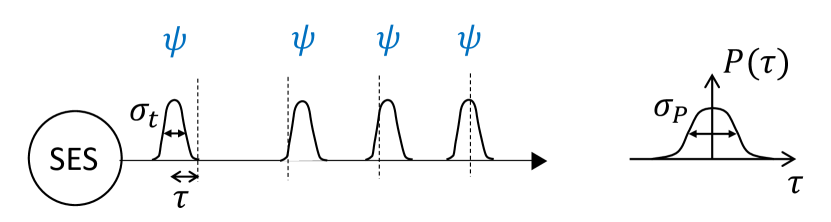
Figure 1: Single-electron sources with timing noise. At each emission (dashed lines), a pure state $\psi$ is temporally translated by random timing shift $\tau$, governed by probability distribution $P(\tau)$.

In this work, we study the decoherence effect induced by timing noise in SESs, see Fig. 1. This noise generates an stochastic ensemble of wave packets which are temporally translated. Thus, the coherence between different energy components are suppressed when the time uncertainty of the noise is much larger than that of the wave packet. We present a protocol to identify the timing noise, i.e., to decide whether a SES involves timing noise and to obtain its noise distribution. Using the proposed protocol, we find that a mixed state whose Wigner distribution is bivariate Gaussian, experimentally detected in quantum-dot SESs [39], is consistent with timing noise. The protocol also enables to extract the time uncertainty of the timing noise that characterizes the noisy SES. We show that an energy filtering can recover the coherence when the time elongation due to the filtering is larger than the time uncertainty of the timing noise.

Single-electron source with timing noise.— Periodically, the source generates a single-electron excitation, described by a pure-state wave packet $\ket{\psi}$ of time uncertainty $\sigma_{t}$ (namely, the position uncertainty divided by the velocity), with random time shifts $\tau$ distributed according to the probability function $P(\tau)$ of variance $\sigma_{P}^{2}$, see Fig. 1. Note that the source generates the excitation in periodic fashion to generate an electric current sufficiently large enough to be measured. We assume that the period $T$ is much larger than the time uncertainties of the excitations to ensure stochastic independence between the periods, $T\gg\sigma_{t},\sigma_{P}$. We also assume that the waveguide into which the SES emits the excitation has a linear dispersion relation between energy and momentum to avoid the wave-packet spreading.

The random timing shift can be caused by various mechanisms, e.g., a jitter in arbitrary waveform generator [36] or by charge fluctuations which affect the potential of the quantum dot, leading to emission delay [41]. In addition, a clock used in the synchronization between the source and the detector (or another SES) has a fundamental error governed by the thermodynamic uncertainty relation [42, 43]. Rather than studying the microscopic mechanism, we focus on the characterization and identification of the state generated by the noisy SES.

The electron state generated by the noisy SES is given by the stochastic ensemble of wave packets $\ket{\psi}$ with different timings, and hence described by the density matrix

$$\rho=\int d\tau\,P(\tau)\hat{\mathbf{T}}(\tau)\ket{\psi}\bra{\psi}\hat{\mathbf{T}}^{\dagger}(\tau).$$ (1)

Here $\hat{\mathbf{T}}(\tau)$ is the translation operator which delays the emission timing by $\tau$. In terms of Wigner distribution, Eq. (1) is equivalent to

$$W(E,t)=\int d\tau\,P(\tau)W_{0}(E,t-\tau).$$ (2)

where $W_{0}$ is the Wigner distribution of the wave packet $\ket{\psi}$, and the connection between the Wigner distribution and the density matrix is $W(E,t)=(2/h)\int d\mathcal{E}\braket{E+\mathcal{E}}{\rho}{E-\mathcal{E}}e^{-i2\mathcal{E}t/\hbar}.$ $W_{0}(E,t)$ is determined by the same equation replacing $\rho$ with $\ket{\psi}\bra{\psi}$. Note that $t$ is the arrival time [37] which is an observable equivalent to position due to the linear dispersion relation.

Equation (1) provides the properties of the mixed state $\rho$ generated by the noisy SES. Due to the convolution form of Eq. (2), the temporal variance of the mixed state, $\Sigma_{t}^{2}\equiv\int dE\,dt\,t^{2}W(E,t)-\{\int dE\,dt\,tW(E,t)\}^{2}$, is the summation of variances of the timing noise and the wave packet,

$$\Sigma_{t}^{2}=\sigma_{P}^{2}+\sigma_{t}^{2},$$ (3)

for any $P(\tau)$ and $\ket{\psi}$. The convolution form also suggests that the coherence stored in different energies is reduced. In fact, the timing noise induces pure dephasing [44, 45, 46, 47] in the energy basis, which can be seen by Fourier transforming Eq. (2),

$$\braket{E}{\rho}{E^{\prime}}=\braket{E}{\psi}\braket{\psi}{E^{\prime}}\int d\tau\,P(\tau)e^{i(E-E^{\prime})\tau/\hbar}.$$ (4)

The integral, i.e., the Fourier transform of $P(\tau)$, equals 1 for $E=E^{\prime}$ [due to the normalization of $P(\tau)$] and decays when the energies $E$ and $E^{\prime}$ differ more than $\hbar/\sigma_{P}$; In the case of Gaussian noise, the integral becomes $e^{-\sigma_{P}^{2}(E-E^{\prime})^{2}/(2\hbar^{2})}$. It follows that timing noise suppresses the off-diagonal elements while keeping the diagonal elements the same, $\braket{\rho}_{E}=|\braket{E}{\psi}|^{2}$. The coherence stored in different energies is almost lost when the variances of the timing noise is much larger than the time uncertainty of $\ket{\psi}$, that is, $\sigma_{P}\gg\sigma_{t}$. This is clearly seen for a Gaussian noise and a Gaussian packet $\psi$, when the quantum purity, $\gamma=\text{Tr}\rho^{2}$, of the mixed state is determined as $\gamma=1/\sqrt{1+(\sigma_{P}/\sigma_{t})^{2}}$.

We put forward a method that not only tells if a SES involves timing noise or not but also provides details about the noise distribution $P(\tau)$ and the wave packet $\ket{\psi}$. Such identification is not a trivial task because the microscopic mechanisms are difficult to be controlled, and neither the noise distribution $P(\tau)$ nor $\ket{\psi}$ are known in advance. Our protocol only relies on the information about the density matrix of $\rho$ which can be obtained from tomography [39]. We assume that the density matrix $\braket{E}{\rho}{E^{\prime}}$ does not have zeros for simplicity; see Supplemental Material (SM) for the general case.

The method is based on the following theorem. A mixed state $\rho$ satisfies Eq. (1) if and only if (i) a function $|\braket{E}{\rho}{E^{\prime}}|/\sqrt{\braket{\rho}_{E}\braket{\rho}_{E^{\prime}}}$ only depends on energy difference $E-E^{\prime}$ and (ii) its Fourier transform with respect to $E-E^{\prime}$ is a positive function, and (iii) $e^{i\text{ arg}\braket{E}{\rho}{E^{\prime}}}$ is a rank-1 matrix. We refer the reader to the SM for the proof. When these conditions hold, the noise distribution $P(\tau)$ and the wave packet $\ket{\psi}$ are uniquely determined in terms of the density matrix as

$$P(\tau)=\frac{1}{h}\int dE\frac{|\braket{\bar{E}+\frac{E}{2}}{\rho}{\bar{E}-\frac{E}{2}}|}{\sqrt{\braket{\rho}_{\bar{E}+\frac{E}{2}}\braket{\rho}_{\bar{E}-\frac{E}{2}}}}e^{-iE\tau/\hbar},$$ (5)

$$\braket{E}{\psi}\braket{\psi}{E^{\prime}}=\sqrt{\braket{\rho}_{E}\braket{\rho}_{E^{\prime}}}e^{i\text{ arg}\braket{E}{\rho}{E^{\prime}}},$$ (6)

where $\bar{E}\equiv\int dE\,E\braket{\rho}_{E}$ is the mean energy.

Using the identification method, we find that a mixed state whose Wigner distribution is bivariate Gaussian is consistent with timing noise. The Wigner distribution is written as

$$W(E,t) = \frac{\exp\left[-\frac{1}{2(1-r)^{2}}\left(\frac{E^{2}}{\Sigma_{E}^{2}}-2r\frac{E}{\Sigma_{E}}\frac{t}{\Sigma_{t}}+\frac{t^{2}}{\Sigma_{t}^{2}}\right)\right]}{2\pi\Sigma_{E}\Sigma_{t}\sqrt{1-r^{2}}},$$ (7)

where $\Sigma_{E}$, $\Sigma_{t}$, and $r$ are the energy, time uncertainties and the energy-time correlation, respectively. These states are observed in Ref. [39] in the regime of fast pumping. One can easily verify the conditions (i)–(iii). Using Eqs. (5) and (6), we obtain both the noise distribution and the wave packet,

$$P(\tau) =\frac{1}{\sqrt{2\pi}\sigma_{P}}e^{-\tau^{2}/(2\sigma_{P}^{2})},$$ (8)

$$\sigma_{P} =\sqrt{(1-r^{2})\Sigma_{t}^{2}-\big{(}\frac{\hbar}{2\Sigma_{E}}\big{)}^{2}}$$ (9)

$$\braket{E}{\psi} =\frac{1}{\sqrt{\sqrt{2\pi}\Sigma_{E}}}\exp\Big{[}-\frac{E^{2}}{4\Sigma_{E}^{2}}+i\frac{r\Sigma_{t}E^{2}}{2\hbar\Sigma_{E}}\Big{]}$$ (10)

Note $\sigma_{P}$ in Eq. (9) is manifestly real due to the fact that the purity is bounded by $1$, $\hbar/[2\sqrt{1-r^{2}}\Sigma_{t}\Sigma_{E}]\leq 1$.

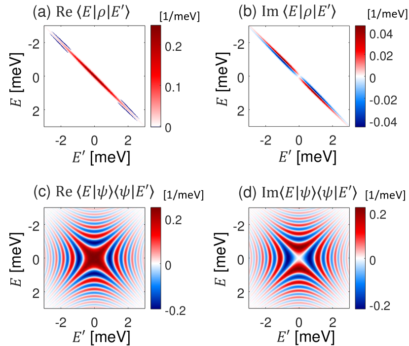
Figure 2: Timing noise identification. (a)–(b) The density matrix in energy basis for the state detected in Ref. [39]. Its Wigner distribution is bivariate Gaussian with $\Sigma_{E}=1.61$ meV, $\Sigma_{t}=6.44$ ps, and $r=0.47$. This state is the result of noisy SES emitting pure-state wave packet $\psi$, (c)–(d), with Gaussian timing noise of uncertainty $\sigma_{P}=5.7$ ps.

Fig. 2 shows the density matrix of $\rho$ and its wave-packet component. It shows that the mixed state, being squeezed along the diagonal in the energy basis [see panels (a) and (b)] is significantly different from the wave-packet component, which exhibits high degree of symmetry [see panels (c) and (d)].

It is worth to mention a peculiarity of bivariate Gaussian Wigner distribution. On one hand, it is consistent with timing noise. On the other hand, because the energy and time appear in equal footing in such distribution, it can also be interpreted by another description of an energy noise. We find that a bivariate Gaussian can be written as $W(E,t)=\int d\mathcal{E}\,\tilde{P}(\mathcal{E})\tilde{W}_{0}(E-\mathcal{E},t)$ where $\tilde{P}(\mathcal{E})$ is a Gaussian noise distribution for random energy shifts applied to a pure-state bivariate Gaussian $\tilde{W}_{0}(E,t)$, see SM. Note that such alternative interpretation is generally impossible for non-Gaussian states; e.g., a state generated by a (zero-temperature) Leviton source with a timing noise can not be explained by another source with the energy noise, see SM. Furthermore, the fact that a bivariate Gaussian state is consistent with timing noise allows for a simple and intuitive purification procedure as follows.

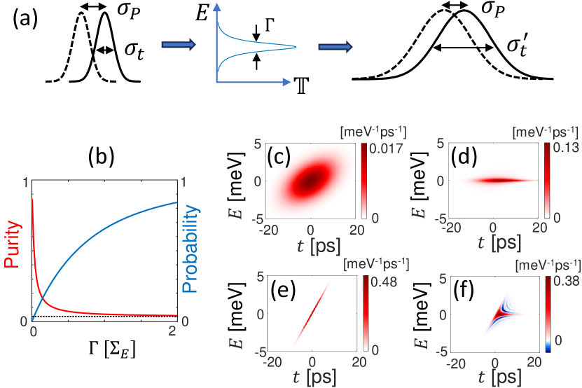
Figure 3: (a) Scheme for the timing noise cancellation using a resonance level. A mixed state generated by temporally noisy SES is energy filtered by a resonance level with broadening $\Gamma$ and becomes elongated in time, reducing the effect of the timing noise. (b) Purity after the filtering $\gamma^{\prime}$ and the packet transmission probability $\mathbb{T}_{0}$. Dotted line: purity before the filtering $\gamma$. (c)–(d) Wigner distribution before and after the filtering at $\Gamma=0.1\Sigma_{E}$. The purity is increased from 0.036 to 0.22 with $12\%$ probability. (e)–(f) Wigner distribution of the pure-state components, $\psi$ and $\psi^{\prime}$, corresponding to (c) and (d). Note that here we show the Wigner distribution instead of the density matrix for a compact visualization but they are equivalent; the panels (c) and (e) are equivalent to Fig. 2. Parameters: the state of Fig. 2 is used for the state before the filtering.

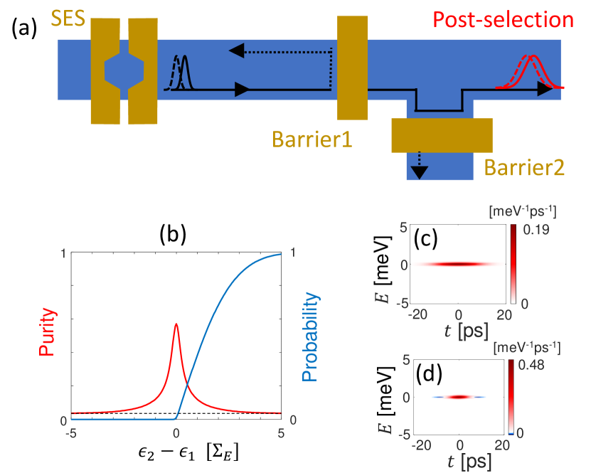
Figure 4: (a) Energy filtering using potential barriers without backscattering between them. The state which has transmitted through the first barrier and reflected at the second one is post-selected. (b) Enhanced purity and the post-selection probability for various barrier height differences $\epsilon_{2}-\epsilon_{1}$. Dashed line: purity before the filtering $\gamma$. (c)–(d) Wigner distribution after the filtering and its pure-state component at $\epsilon_{2}-\epsilon_{1}=0.2\Sigma_{E}$ where the purity is enhanced from 0.036 to 0.41 with $8\%$ probability. Parameter: $\Delta_{b}=0.03\Sigma_{E}$ and the state of Fig. 2 is used for the state before the filtering.

Cancelling timing noise.— Luckily, the coherence loss due to timing noise can be recovered. The purity reduction is determined by the competition of noise time uncertainty $\sigma_{P}$ and the quantum time uncertainty $\sigma_{t}$. Consider a dynamic mapping which changes the packet $\psi$ to another pure state $\psi^{\prime}$ which is elongated in time, so that the new time uncertainty $\sigma_{t}^{\prime}$ is larger than the original value $\sigma_{t}$. If the dynamic mapping commutes with the time-translation operator $\hat{\mathbf{T}}(\tau)$, the mapping changes the mixed state $\rho$ to

$$\rho^{\prime}=\int d\tau\,P(\tau)\hat{\mathbf{T}}(\tau)\ket{\psi^{\prime}}\bra{\psi^{\prime}}\hat{\mathbf{T}}^{\dagger}(\tau).$$ (11)

Then, the new purity $\gamma^{\prime}=\text{Tr}(\rho^{\prime})^{2}$ becomes larger than the original purity $\gamma=\text{Tr}\rho^{2}$ since the relative strength of the timing noise is weaker, namely, $\sigma_{P}/\sigma_{t}^{\prime}<\sigma_{P}/\sigma_{t}$. Note that $\sigma_{t}^{\prime}$ should be smaller than the SES period to ensure the interperiod independence.

Such dynamic mapping should be nonunitary because a unitary operation conserves the purity. Additionally, $\psi^{\prime}$ should have smaller energy uncertainty than $\psi$ in order to have larger time uncertainty. Therefore, a natural option for the dynamic mapping is energy filtering. This energy filtering can be realized by postselecting a state transmitted through a single resonance level with a large lifetime (i.e., small resonance width $\Gamma$), see Fig. 3(a). The state post-selected by the energy filtering is described by Eq. (11) with

$$\ket{\psi^{\prime}}=\frac{1}{\sqrt{\mathbb{T}_{0}}}\int dE\,\ket{E}\braket{E}{\psi}\mathbb{t}(E)$$ (12)

where $\mathbb{t}(E)$ is the transmission amplitude, $\mathbb{T}(E)\equiv|\mathbb{t}(E)|^{2}$, and $\mathbb{T}_{0}=\int dE\,|\braket{E}{\psi}|^{2}\mathbb{T}(E)$ is the transmission probability for the packet.

In Fig. 3 we show the result of calculations using the transmission probability $\mathbb{T}(E)=1/[1+E^{2}/\Gamma^{2}]$, where energy is measured from the resonance level. For simplicity, we focus on the case that the mean energy of $\rho$ is aligned with the resonance level (see SM for different cases). Panel (b) in Fig. 3 shows the purity $\gamma^{\prime}$ after filtering a bivariate-Gaussian Wigner distribution as observed in Ref. [39]. The purity approaches 1 as the level broadening $\Gamma$ is reduced. However, a sharp filtering accompanies the weaker signal, manifested in the trade-off relation shown in the transmission probability and the state deformation. One should select the value of $\Gamma$ with a compromise. For example, when $\Gamma=0.1\Sigma_{E}$, the purity is significantly enhanced from $\sim 0.04$ to $\sim 0.2$ with $10\%$ probability, without completely deforming the state [see Fig. 3(c)-(d)]. Note that the situation of single-resonance level can be implemented using a Fabry-Pérot interferometer (or a quantum dot) with a resonance-level spacing much larger than the energy uncertainty of the state before filtering.

The Fabry-Pérot interferometer often involves complications from Coulomb interactions [48, 49, 50, 51]. Instead, energy filtering can also be realized by a three-lead junction with two potential barriers without backscattering between them, readily implementable in the experiments. Here the state after the transmission and subsequent reflection is post-selected. The transmission probability of the first [second] barrier is $1/(1+\exp\{-(E-\epsilon_{1[2]})/\Delta_{b}\})$ [52]. We assume $\Delta_{b}\ll\Sigma_{E}$ to have sufficient filtering effect and ignore the small phase variation [53] in the tunneling amplitude over the energy window $E\in[\epsilon_{n}-\Delta_{b},\epsilon_{n}+\Delta_{b}]$. Fig. 4(b)–(d) shows the result, focusing on the case that $\Delta_{b}=0.03\Sigma_{E}$ and $(\epsilon_{1}+\epsilon_{2})/2=\braket{E}_{\rho}$; see SM for other cases. Similarly to the result of Fig. 3, we obtain a significant purity enhancement with sufficient probability, e.g., the purity is enhanced from $\sim 0.04$ to $\sim$ 0.4 with $8\%$ probability at $\Delta_{b}=0.03\Sigma_{E}$ and $\epsilon_{2}-\epsilon_{1}=0.2\Sigma_{E}$. The detailed form of the post-selected packet $\ket{\psi^{\prime}}$ shown in Fig. 4(d) differs from that of Fig. 3(f) due to the different forms of the transmission amplitude $\mathbb{t}(E)$ (rectangular function for the former and simple pole for the latter).

Discussion.— We have developed a theory for timing noise present in single-electron sources. Timing noise induces a pure dephasing in energy basis. This fact provides a method for identifying SES with such noise, extracting information about the noise, and allows for a simple and experimentally accessible purification procedure based on energy filtering. In the case of a bivariate Gaussian Wigner distribution, which describes the experimental data in Ref. [39], our work does not exclude other causes but timing noise is a most simple and natural explanation.

Our theory implies that a programmed timing noise will be a useful tool for realizing pure dephasing in energy basis. Such programming may be realized using a noisy clock for voltage pulses applied to SESs. By tuning the noise strength, namely, the time uncertainty $\sigma_{P}$, one can change the coherence (i.e., the off-diagonal elements of the density matrix in the energy basis) without changing the population in energy (i.e., the diagonal elements). This will open the way to answer a compelling question in quantum thermodynamics: what is the effect of coherence in the functionalities of nanoscale thermal machines [54, 55]? Studies in quantum thermodynamics have revealed intriguing roles of quantum coherence, sometimes offering quantum advantages with regard to the quantum-dephased case but it is unclear how the dephased system can be prepared [56, 57, 58, 59]. The tunable pure dephasing proposed here will also assist in the recent quest of electron quantum optics, providing a way to distinguish Coulomb interaction effects and exchange effects in Hong-Ou-Mandel-type collision experiments [28, 29, 30]. A controllability of the timing noise will enable tuning the exchange effect without affecting Coulomb interaction, since a small timing noise will not alter the Coulomb effects much.

Acknowledgments.—This work was partially supported by the Spanish State Research Agency (MCIN/AEI/10.13039/501100011033) and FEDER (UE) under Grant No. PID2020-117347GB-I00 and the María de Maeztu project CEX2021-001164-M, and by CSIC/IUCRAN2022 under Grant No. UCRAN20029. SR acknowledges a partial support from UIB through the research project led by a postdoctoral principal investigator.

This material contains the derivation of the theorem for identifying the timing noise and detailed results about the timing noise cancellation.

S1 Derivation of the theorem for identifying the timing noise

Here we show the proof of the theorem used for the identification of the timing noise in the main text.

S1.1 Simple case

As assumed in the main text, we first consider the simple case that the density matrix $\braket{E}{\rho}{E^{\prime}}$ does not have any zero.

Theorem: If there is no zero of $\braket{E}{\rho}{E^{\prime}}$, Eq. (1) holds if and only if (i) a function $|\braket{E}{\rho}{E^{\prime}}|/\sqrt{\braket{\rho}_{E}\braket{\rho}_{E^{\prime}}}$ only depends on the energy difference $E-E^{\prime}$ and (ii) its dependence has a positive Fourier transform, and (iii) $e^{i\text{arg}\braket{E}{\rho}{E^{\prime}}}$ is rank-1 matrix.

Proof. We first show that the conditions (i)–(iii) are necesary for Eq. (1). Using $\hat{\mathbf{T}}(\tau)\ket{E}=e^{iE\tau/\hbar}\ket{E}$, Eq. (1) is equivalent to

$$\braket{E}{\rho}{E^{\prime}}=g(E-E^{\prime})\braket{E}{\chi}{E^{\prime}},$$ (S1)

where $g(E)\equiv\int d\tau P(\tau)e^{iE\tau/\hbar}$ is the Fourier transform of the timing noise distribution $P(\tau)$ and $\chi\equiv\ket{\psi}\bra{\psi}$ is the density matrix describing the pure state $\ket{\psi}$ which appears in Eq. (1). $g(0)=1$ due to the normalization of $P(\tau)$. Then, $g(E)$ should be a continuous function because $\braket{E}{\rho}{E^{\prime}}$ and $\braket{E}{\chi}{E^{\prime}}$ are continuous functions with respect to $E$ and $E^{\prime}$. Furthermore, $g(E)$ should be a positive function because otherwise it contradicts the assumption that there is no zero of $\braket{E}{\rho}{E^{\prime}}$. Using Eq. (S1), the positivity of $g(E)$, the property of the pure state $|\braket{E}{\chi}{E^{\prime}}|=\sqrt{\braket{\chi}_{E}\braket{\chi}_{E^{\prime}}}$, and $\braket{\chi}_{E}=\braket{\rho}_{E}$, we obtain the condition (i) because

$$\frac{|\braket{E}{\rho}{E^{\prime}}|}{\sqrt{\braket{\rho}_{E}\braket{\rho}_{E^{\prime}}}} =g(E-E^{\prime}).$$ (S2)

The condition (ii) is also satisfied because the Fourier transform of Eq. (S2) equals $P(\tau)$ which is a positive function by definition. The condition (iii) is also satisfied because $e^{i\text{ arg}\braket{E}{\rho}{E^{\prime}}}$ can be written in a product form, $e^{i\text{ arg}\braket{E}{\rho}{E^{\prime}}}=e^{i\text{ arg}\braket{E}{\chi}{E^{\prime}}}=e^{i\text{ arg}\braket{E}{\psi}}e^{i\text{ arg}\braket{\psi}{E^{\prime}}}$.

Now I show that the conditions (i)–(iii) are the sufficient for Eq. (1). We choose ansatzes for the pure state $\chi$ and the Fourier transform of the timing noise distribution as

$$\braket{E}{\chi_{a}}{E^{\prime}} \equiv\sqrt{\braket{\rho}_{E}\braket{\rho}_{E^{\prime}}}e^{i\text{ arg}\braket{E}{\rho}{E^{\prime}}},$$ (S3)

$$g_{a}(E-E^{\prime}) \equiv\frac{|\braket{E}{\rho}{E^{\prime}}|}{\sqrt{\braket{\rho}_{E}\braket{\rho}_{E^{\prime}}}},$$ (S4)

respectively. Note that the condition (i) is used to define $g_{a}(E-E^{\prime})$. The ansatz satisfies

$$\braket{E}{\rho}{E^{\prime}}=g_{a}(E-E^{\prime})\braket{E}{\chi_{a}}{E^{\prime}}.$$ (S5)

In the same way that Eq. (S1) is equivalent to Eq. (1), Eq. (S5) is equivalent to

$$\rho=\int d\tau\,P_{a}(\tau)\mathbf{T}(\tau)\chi_{a}\mathbf{T}^{\dagger}(\tau).$$ (S6)

where $P_{a}(\tau)\equiv\int d\mathcal{E}\,g_{a}(\mathcal{E})e^{-i\mathcal{E}\tau/\hbar}/h$ corresponds to the ansatz for noise distribution $P(\tau)$. Eq. (S6) implies that the ansatzes are correct if $P_{a}(\tau)$ and $\chi_{a}$ describe a noise distribution and a pure state, respectively. This is the case because $P_{a}(\tau)$ is a positive function due to the condition (ii), $\int P_{a}(\tau)d\tau=1$ due to $g_{a}(0)=1$ [see Eq. (S4)], and $\chi_{a}$ is a pure state due to the condition (iii). $\square$

Note that Eqs. (S1) and  (S2) imply that the pure state $\chi$ and the timing noise distribution $P(\tau)$ for a given mixed state are unique and determined as,

$$\braket{E}{\chi}{E^{\prime}} =\sqrt{\braket{\rho}_{E}\braket{\rho}_{E^{\prime}}}e^{i\text{ arg}\braket{E}{\rho}{E^{\prime}}},$$ (S7)

$$P(\tau) =\frac{1}{h}\int dE\frac{|\braket{\bar{E}+\frac{E}{2}}{\rho}{\bar{E}-\frac{E}{2}}|}{\sqrt{\braket{\rho}_{\bar{E}+\frac{E}{2}}\braket{\rho}_{\bar{E}-\frac{E}{2}}}}e^{-iE\tau/\hbar},$$ (S8)

where $\bar{E}\equiv\int dE\,E\braket{\rho}_{E}$ is the electron mean energy.

S1.2 General case

When the density matrix $\braket{E}{\rho}{E^{\prime}}$ has any zero, the derivation in Sec. S1.1 is not valid because $g(E-E^{\prime})$ in Eq. (S1) is not guaranteed to be positive. We show how to generalize the theorem.

We first observe the property of the possible zeros of state generated by the timing noise. Eq. (S1), which is equivalent to Eq. 1, implies that the zeros of $\braket{E}{\rho}{E^{\prime}}$ originate from either $g(E-E^{\prime})$ or $\braket{E}{\chi}{E^{\prime}}$. The former type of zeros is determined by the character of the timing noise. For example when the timing noise distribution $P(\tau)$ is rectangular function with width $w$, its Fourier transform $g(E-E^{\prime})$ has zeros at $|E-E^{\prime}|=nh/w$ for integer $n$. Note that $g(E-E^{\prime})$ has zeros distributed symmetrically with respect to $E-E^{\prime}=0$, because $P(\tau)$ and $g(E-E^{\prime})$ are a real and even function. We denote $n$th zero of $g(E-E^{\prime})$ counted from $|E-E^{\prime}|=0$ as $z_{n}$, namely $g(E-E^{\prime})=0$ for $|E-E^{\prime}|=z_{n}$ and $z_{1}<z_{2}<\cdots$. These zeros result in the zeros of the density matrix $\braket{E}{\rho}{E^{\prime}}$ spread over diagonals, i.e., $\braket{E}{\rho}{E^{\prime}}=0$ along the lines satisfying $|E-E^{\prime}|=z_{n}$.

The other type of zeros is determined by the zero of $\braket{E}{\chi}{E^{\prime}}$. These zeros are determined by the character of the pure state $\ket{\psi}$, for example as a result of destructive interference. We denote $m$th zero of $\braket{E}{\psi}$ as $\zeta_{m}$, namely $\braket{E}{\psi}=0$ for $E=\zeta_{m}$. These zeros result in the zeros of the density matrix $\braket{E}{\rho}{E^{\prime}}$ spread over a horizontal and vertical lines which cross at the main diagonal, i.e., $\braket{E}{\rho}{E^{\prime}}=0$ for $E=\zeta_{m}$ or $E^{\prime}=\zeta_{m}$.

For the theorem below, we denote the sign $g(\mathcal{E})$ as $\lambda(\mathcal{E})$, namely $\lambda(\mathcal{E})\equiv 1$ when $g(\mathcal{E})\geq 0$ and -1 otherwise. Due to the property of the zeros of $\rho$, the function $\lambda(\mathcal{E})$ can be determined by observing the density matrix $\braket{E}{\rho}{E^{\prime}}$ and using the following procedure. Firstly, $\lambda(0)=1$ because $g(0)=1$ due to the normalization of $P(\tau)$. And one can locate the positions of the change of signs of $\lambda(\mathcal{E})$, using the fact that a sign change occurs across the diagonal-type zeros of $\braket{E}{\rho}{E^{\prime}}$, namely across $\mathcal{E}=\pm z_{n}$, which accompany the $\pi$-phase shift in the density matrix $\braket{E}{\rho}{E^{\prime}}$.

Now we present the theorem for identifying the timing noise, expressed in terms of the density matrix $\braket{E}{\rho}{E^{\prime}}$, the positions of its zeros $z_{n}$, and the sign function $\lambda$ which can be extracted from the density matrix, hence relying only on the information of the density matrix. The theorem and its derivation are slightly modified from those of Sec. S1.1.

Theorem: Eq. (1) holds if and only if (i) a matrix

$$\frac{|\braket{E}{\rho}{E^{\prime}}|}{\sqrt{\braket{\rho}_{E}\braket{\rho}_{E^{\prime}}}}\lambda(E-E^{\prime})$$ (S9)

only depends on energy difference $E-E^{\prime}$, (ii) its dependence has a positive Fourier transform, (iii) $e^{i\text{arg}\braket{E}{\rho}{E^{\prime}}}\lambda(E-E^{\prime})$ is rank-1 matrix.

Proof. I first show that the conditions (i)–(iii) are necessary for Eq. (1). Using Eq. (S1), $\lambda(\mathcal{E})=\text{sgn}[g(\mathcal{E})]$, the property of a pure state $|\braket{E}{\chi}{E^{\prime}}|=\sqrt{\braket{\chi}_{E}\braket{\chi}_{E^{\prime}}}$, and $\braket{\chi}_{E}=\braket{\rho}_{E}$, we find that

$$\frac{|\braket{E}{\rho}{E^{\prime}}|}{\sqrt{\braket{\rho}_{E}\braket{\rho}_{E^{\prime}}}}\lambda(E-E^{\prime}) =g(E-E^{\prime}).$$ (S10)

Hence the condition (i) is satisfied. The condition (ii) is also satisfied because the Fourier transform of Eq. (S10) equals $P(\tau)$ which is a positive function by definition. The condition (iii) is also satisfied because $\lambda(E-E^{\prime})e^{i\text{ arg}\braket{E}{\rho}{E^{\prime}}}=e^{i\text{ arg}\braket{E}{\chi}{E^{\prime}}}$ which is a rank-1 matrix.

Now I show that the conditions (i)–(iii) are the sufficient for Eq. (S1). We choose ansatzes for the pure state $\chi$ and the Fourier transform of the timing noise distribution as

$$\braket{E}{\chi_{a}}{E^{\prime}} =\sqrt{\braket{\rho}_{E}\braket{\rho}_{E^{\prime}}}e^{i\text{ arg}\braket{E}{\rho}{E^{\prime}}}\lambda(E-E^{\prime}),$$ (S11)

$$g_{a}(E-E^{\prime}) =\frac{|\braket{E}{\rho}{E^{\prime}}|}{\sqrt{\braket{\rho}_{E}\braket{\rho}_{E^{\prime}}}}\lambda(E-E^{\prime}).$$ (S12)

Note that the condition (i) is used to define $g_{a}(E-E^{\prime})$. The ansatzes satisfy

$$g_{a}(E-E^{\prime})\braket{E}{\chi_{a}}{E^{\prime}}=\braket{E}{\rho}{E^{\prime}}.$$ (S13)

Its Fourier transform gives

$$\rho=\int d\tau\,P_{a}(\tau)\mathbf{T}(\tau)\chi_{a}\mathbf{T}^{\dagger}(\tau).$$ (S14)

Here $P_{a}(\tau)\equiv\int d\mathcal{E}\,g_{a}(\mathcal{E})e^{-i\mathcal{E}\tau/\hbar}/h$ corresponds to the ansatz for noise distribution $P(\tau)$. Eq. (S14) implies that the ansatzes are correct if $P_{a}(\tau)$ and $\chi_{a}$ describe a noise distribution and a pure state, respectively. This is the case because $P_{a}(\tau)$ is a positive function due to the condition (ii), $\int P_{a}(\tau)d\tau=1$ due to $g_{a}(0)=1$ [see Eq. (S12)], and $\chi_{a}$ is a pure state due to the condition (iii). $\square$

Note that Eqs. (S1) and  (S10) imply that $\chi$ and $P(\tau)$ for a temporally noisy state are unique and determined as,

$$\braket{E}{\chi}{E^{\prime}} =\sqrt{\braket{\rho}_{E}\braket{\rho}_{E^{\prime}}}e^{i\text{ arg}\braket{E}{\rho}{E^{\prime}}}\lambda(E-E^{\prime}),$$ (S15)

$$P(\tau) =\frac{1}{h}\int dE\frac{|\braket{\bar{E}+\frac{E}{2}}{\rho}{\bar{E}-\frac{E}{2}}|}{\sqrt{\braket{\rho}_{\bar{E}+\frac{E}{2}}\braket{\rho}_{\bar{E}-\frac{E}{2}}}}\lambda(E)e^{-iE\tau/\hbar},$$ (S16)

where $\bar{E}\equiv\int dE\,E\braket{\rho}_{E}$ is the mean energy.

S2 Bivariate Gaussian Wigner function

Here we show an alternative interpretation of bivariate Gaussian Wigner function using the energy noise instead of the timing noise.

We find that a mixed state whose Wigner function is bivariate Gaussian, see Eq. (7), can be written as

$$W(E,t)=\int d\mathcal{E}\tilde{P}(\mathcal{E})\tilde{W}_{0}(E-\mathcal{E},t).$$ (S17)

$\tilde{P}(\mathcal{E})$ is Gaussian distribution describing a random energy shift, instead of the timing shift, with uncertainty $\xi$ given to SES,

$$\tilde{P}(\mathcal{E}) =\frac{1}{\sqrt{2\pi}\xi}e^{-\mathcal{E}^{2}/(2\xi^{2})},$$ (S18)

$$\xi =\sqrt{(1-r^{2})\Sigma_{E}^{2}-\big{(}\frac{\hbar}{2\Sigma_{t}}\big{)}^{2}}.$$ (S19)

We recall that $\Sigma_{E}$,$\Sigma_{t}$, and $r$ are energy uncertainty, time uncertainty, and energy-time correlation of $W(E,t)$, respectively. $\xi$ in Eq. (S19) is manifestly real due to the fact that the purity of $W$ is bounded by 1, $\hbar/[2\sqrt{1-r^{2}}\Sigma_{t}\Sigma_{E}]\leq 1$. $\tilde{W}_{0}$ is a pure-state Wigner function determined as

$$\tilde{W}_{0}(E,t)=\frac{2}{h}\exp\Big{[}-\big{(}\frac{1}{2\Sigma_{t}^{2}}+\frac{2r^{2}\Sigma_{E}^{2}}{\hbar^{2}}\big{)}t^{2}+\frac{4r\Sigma_{E}\Sigma_{t}}{\hbar^{2}}tE-2\frac{\Sigma_{t}^{2}}{\hbar^{2}}E^{2}].$$ (S20)

One can check easily that the purity of Eq. S20 is unity, $h\int dE\,dt\,\tilde{W}_{0}^{2}(E,t)=1$. As mentioned in the main text, such alternative interpretation is a consequence of the fact that a bivariate Gaussian Wigner function has energy and time dependence in equal footing; Eqs. (S17)–(S20) are equivalent to Eqs. (2),(8),(9), and (10) when exchanging the role of energy and time.

S3 Extended results of Fig. 3 and 4.

Here we show how the results of Fig. 3 and 4 in the main text extend for different parameters.

Fig. S1 shows how the result of Fig. 3, where a resonance level is used for the timing noise cancellation, extends when the energy of the resonance level $\epsilon_{0}$ is not aligned with the packet mean energy $\bar{E}$. In this case, the transmission probability through the resonance level is $\mathbb{T}(E)=1/[1+(E-\epsilon_{0})^{2}/\Gamma^{2}]$. The result shows that as the resonance level deviates from the packet mean energy, both the filtered purity and the probability both decrease. This indicates that it is best to align the resonance level with the packet mean energy for the timing noise cancellation. However, as long as the resonance level is near the mean energy, $\epsilon_{0}\in[\bar{E}-\Sigma_{E},\bar{E}+\Sigma_{E}]$, the timing noise cancellation is achieved with almost the same results.

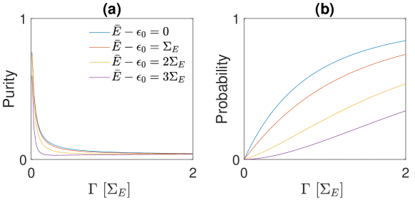
Figure S1: Timing noise cancellation using a resonance level for various mean energy $\bar{E}$ of the packet measured with respect to the resonance level $\epsilon_{0}$. (a) Purity after the energy filtering through the resonance level. (b) Packet transmission probability. The parameters used for the result are the same as Fig. 3 except $\bar{E}-\epsilon_{0}$. The lines with $\bar{E}-\epsilon_{0}=0$ (blue) correspond to the result of Fig. 3(b).

Fig. S2 shows how the result of Fig. 4, where a potential barriers are used for the timing noise cancellation, extends when the broadening of the barrier, $\Delta_{b}$, is varied. As $\Delta_{b}$ increases, the purity decreases while the probability slightly increases. This indicates that it is best to use the barriers with small $\Delta_{b}$, which corresponding to thick barrier width, for the timing noise cancellation. And as long as $\Delta_{b}$ is much smaller than the energy uncertainty $\Sigma_{E}$, the timing noise cancellation is achieved with similar results.

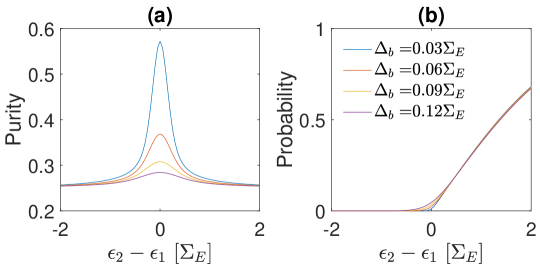
Figure S2: Timing noise cancellation using a potentical barriers for various broadening $\Delta_{b}$. (a) Purity after the energy filtering through the barriers. (b) Post-selection probability. The parameters used for the results are the same as Fig. 4 except $\Delta_{b}$. The lines with $\Delta E_{b}=0.03\Sigma_{E}$ (blue) correspond to the result of Fig. 4(b).

References

- Cabart et al. [2018] C. Cabart, B. Roussel, G. Fève, and P. Degiovanni, Taming electronic decoherence in one-dimensional chiral ballistic quantum conductors, Phys. Rev. B 98, 155302 (2018).
- Das Sarma and Madhukar [1980] S. Das Sarma and A. Madhukar, Study of electron-phonon interaction and magneto-optical anomalies in two-dimensionally confined systems, Phys. Rev. B 22, 2823 (1980).
- Taubert et al. [2011] D. Taubert, C. Tomaras, G. J. Schinner, H. P. Tranitz, W. Wegscheider, S. Kehrein, and S. Ludwig, Relaxation of hot electrons in a degenerate two-dimensional electron system: Transition to one-dimensional scattering, Phys. Rev. B 83, 235404 (2011).
- Ji et al. [2003] Y. Ji, Y. Chung, D. Sprinzak, M. Heiblum, D. Mahalu, and H. Shtrikman, An electronic Mach-Zehnder interferometer, Nature 422, 415 (2003).
- McClure et al. [2009] D. T. McClure, Y. Zhang, B. Rosenow, E. M. Levenson-Falk, C. M. Marcus, L. N. Pfeiffer, and K. W. West, Edge-State Velocity and Coherence in a Quantum Hall Fabry-Pérot Interferometer, Phys. Rev. Lett. 103, 206806 (2009).
- Splettstoesser and Haug [2017] J. Splettstoesser and R. J. Haug, Single-electron control in solid state devices, Physica Status Solidi (b) 254, 1770217 (2017).
- Bäuerle et al. [2018] C. Bäuerle, D. C. Glattli, T. Meunier, F. Portier, P. Roche, P. Roulleau, S. Takada, and X. Waintal, Coherent control of single electrons: a review of current progress, Rep. Prog. Phys. 81, 056503 (2018).
- Pekola et al. [2013] J. P. Pekola, O.-P. Saira, V. F. Maisi, A. Kemppinen, M. Möttönen, Y. A. Pashkin, and D. V. Averin, Single-electron current sources: Toward a refined definition of the ampere, Rev. Mod. Phys. 85, 1421 (2013).
- Keeling et al. [2006] J. Keeling, I. Klich, and L. S. Levitov, Minimal Excitation States of Electrons in One-Dimensional Wires, Phys. Rev. Lett. 97, 116403 (2006).
- Dubois et al. [2013] J. Dubois, T. Jullien, F. Portier, P. Roche, A. Cavanna, Y. Jin, W. Wegscheider, P. Roulleau, and D. C. Glattli, Minimal-excitation states for electron quantum optics using levitons, Nature 502, 659 (2013).
- Féve et al. [2007] G. Féve, A. Mahé, J.-M. Berroir, T. Kontos, B. Plaçais, D. C. Glattli, A. Cavanna, B. Etienne, and Y. Jin, An On-Demand Coherent Single-Electron Source, Science 316, 1169 (2007).
- Moskalets et al. [2008] M. Moskalets, P. Samuelsson, and M. Büttiker, Quantized Dynamics of a Coherent Capacitor, Phys. Rev. Lett. 100, 086601 (2008).
- Keeling et al. [2008] J. Keeling, A. V. Shytov, and L. S. Levitov, Coherent Particle Transfer in an On-Demand Single-Electron Source, Phys. Rev. Lett. 101, 196404 (2008).
- Giblin et al. [2012] S. P. Giblin, M. Kataoka, J. D. Fletcher, P. See, T. J. B. M. Janssen, J. P. Griffiths, G. a. C. Jones, I. Farrer, and D. A. Ritchie, Towards a quantum representation of the ampere using single electron pumps, Nat. Commun. 3, 930 (2012).
- Kaestner and Kashcheyevs [2015] B. Kaestner and V. Kashcheyevs, Non-adiabatic quantized charge pumping with tunable-barrier quantum dots: a review of current progress, Rep. Prog. Phys. 78, 103901 (2015).
- Ryu et al. [2016] S. Ryu, M. Kataoka, and H.-S. Sim, Ultrafast Emission and Detection of a Single-Electron Gaussian Wave Packet: A Theoretical Study, Phys. Rev. Lett. 117, 146802 (2016).
- Hermelin et al. [2011] S. Hermelin, S. Takada, M. Yamamoto, S. Tarucha, A. D. Wieck, L. Saminadayar, C. Bäuerle, and T. Meunier, Electrons surfing on a sound wave as a platform for quantum optics with flying electrons, Nature 477, 435 (2011).
- Kataoka et al. [2009] M. Kataoka, M. R. Astley, A. L. Thorn, D. K. L. Oi, C. H. W. Barnes, C. J. B. Ford, D. Anderson, G. A. C. Jones, I. Farrer, and D. A. Ritchie, Coherent time evolution of a single-electron wave function, Phys. Rev. Lett. 102, 156801 (2009).
- Kataoka et al. [2011] M. Kataoka, J. D. Fletcher, P. See, S. P. Giblin, T. J. B. M. Janssen, J. P. Griffiths, G. A. C. Jones, I. Farrer, and D. A. Ritchie, Tunable Nonadiabatic Excitation in a Single-Electron Quantum Dot, Phys. Rev. Lett. 106, 126801 (2011).
- Yamahata et al. [2019] G. Yamahata, S. Ryu, N. Johnson, H.-S. Sim, A. Fujiwara, and M. Kataoka, Picosecond coherent electron motion in a silicon single-electron source, Nat. Nanotechnol. 14, 1019 (2019).
- Bocquillon et al. [2012] E. Bocquillon, F. D. Parmentier, C. Grenier, J.-M. Berroir, P. Degiovanni, D. C. Glattli, B. Plaçais, A. Cavanna, Y. Jin, and G. Féve, Electron Quantum Optics: Partitioning Electrons One by One, Phys. Rev. Lett. 108, 196803 (2012).
- Bocquillon et al. [2013] E. Bocquillon, V. Freulon, J.-M. Berroir, P. Degiovanni, B. Plaçais, A. Cavanna, Y. Jin, and G. Féve, Coherence and Indistinguishability of Single Electrons Emitted by Independent Sources, Science 339, 1054 (2013).
- Wahl et al. [2014] C. Wahl, J. Rech, T. Jonckheere, and T. Martin, Interactions and Charge Fractionalization in an Electronic Hong-Ou-Mandel Interferometer, Phys. Rev. Lett. 112, 046802 (2014).
- Grenier et al. [2013] C. Grenier, J. Dubois, T. Jullien, P. Roulleau, D. C. Glattli, and P. Degiovanni, Fractionalization of minimal excitations in integer quantum Hall edge channels, Phys. Rev. B 88, 085302 (2013).
- Jonckheere et al. [2023] T. Jonckheere, J. Rech, B. Grémaud, and T. Martin, Anyonic Statistics Revealed by the Hong-Ou-Mandel Dip for Fractional Excitations, Phys. Rev. Lett. 130, 186203 (2023).
- Ubbelohde et al. [2015] N. Ubbelohde, F. Hohls, V. Kashcheyevs, T. Wagner, L. Fricke, B. Kästner, K. Pierz, H. W. Schumacher, and R. J. Haug, Partitioning of on-demand electron pairs, Nat. Nanotechnol. 10, 46 (2015).
- Ryu and Sim [2022] S. Ryu and H.-S. Sim, Partition of Two Interacting Electrons by a Potential Barrier, Phys. Rev. Lett. 129, 166801 (2022).
- Fletcher et al. [2023] J. D. Fletcher, W. Park, S. Ryu, P. See, J. P. Griffiths, G. a. C. Jones, I. Farrer, D. A. Ritchie, H.-S. Sim, and M. Kataoka, Time-resolved Coulomb collision of single electrons, Nat. Nanotechnol. 18, 727 (2023).
- Ubbelohde et al. [2023] N. Ubbelohde, L. Freise, E. Pavlovska, P. G. Silvestrov, P. Recher, M. Kokainis, G. Barinovs, F. Hohls, T. Weimann, K. Pierz, and V. Kashcheyevs, Two electrons interacting at a mesoscopic beam splitter, Nat. Nanotechnol. 18, 733 (2023).
- Wang et al. [2023] J. Wang, H. Edlbauer, A. Richard, S. Ota, W. Park, J. Shim, A. Ludwig, A. D. Wieck, H.-S. Sim, M. Urdampilleta, T. Meunier, T. Kodera, N.-H. Kaneko, H. Sellier, X. Waintal, S. Takada, and C. Bäuerle, Coulomb-mediated antibunching of an electron pair surfing on sound, Nat. Nanotechnol. 18, 721 (2023).
- Gabelli et al. [2006] J. Gabelli, G. Fève, J.-M. Berroir, B. Plaçais, A. Cavanna, B. Etienne, Y. Jin, and D. C. Glattli, Violation of Kirchhoff’s laws for a coherent RC circuit, Science 313, 499 (2006).
- Ferraro et al. [2014] D. Ferraro, B. Roussel, C. Cabart, E. Thibierge, G. Féve, C. Grenier, and P. Degiovanni, Real-Time Decoherence of Landau and Levitov Quasiparticles in Quantum Hall Edge Channels, Phys. Rev. Lett. 113, 166403 (2014).
- Acciai et al. [2022] M. Acciai, P. Roulleau, I. Taktak, D. C. Glattli, and J. Splettstoesser, Influence of channel mixing in fermionic Hong-Ou-Mandel experiments, Phys. Rev. B 105, 125415 (2022).
- Iyoda et al. [2014] E. Iyoda, T. Kato, K. Koshino, and T. Martin, Dephasing in single-electron generation due to environmental noise probed by Hong-Ou-Mandel interferometry, Phys. Rev. B 89, 205318 (2014).
- Blumenthal et al. [2007] M. D. Blumenthal, B. Kaestner, L. Li, S. P. Giblin, T. J. B. M. Janssen, M. Pepper, D. Anderson, G. A. C. Jones, and D. A. Ritchie, Gigahertz quantized charge pumping, Nature Physics 3, 343 (2007).
- Fletcher et al. [2013] J. D. Fletcher, P. See, H. Howe, M. Pepper, S. P. Giblin, J. P. Griffiths, G. A. C. Jones, I. Farrer, D. A. Ritchie, T. J. B. M. Janssen, and M. Kataoka, Clock-Controlled Emission of Single-Electron Wave Packets in a Solid-State Circuit, Phys. Rev. Lett. 111, 216807 (2013).
- Emary et al. [2016] C. Emary, A. Dyson, S. Ryu, H.-S. Sim, and M. Kataoka, Phonon emission and arrival times of electrons from a single-electron source, Phys. Rev. B 93, 035436 (2016).
- Johnson et al. [2018] N. Johnson, C. Emary, S. Ryu, H.-S. Sim, P. See, J. D. Fletcher, J. P. Griffiths, G. A. C. Jones, I. Farrer, D. A. Ritchie, M. Pepper, T. J. B. M. Janssen, and M. Kataoka, LO-Phonon Emission Rate of Hot Electrons from an On-Demand Single-Electron Source in a GaAs/AlGaAs Heterostructure, Phys. Rev. Lett. 121, 137703 (2018).
- Fletcher et al. [2019] J. D. Fletcher, N. Johnson, E. Locane, P. See, J. P. Griffiths, I. Farrer, D. A. Ritchie, P. W. Brouwer, V. Kashcheyevs, and M. Kataoka, Continuous-variable tomography of solitary electrons, Nature Communications 10, 5298 (2019).
- Jullien et al. [2014] T. Jullien, P. Roulleau, B. Roche, A. Cavanna, Y. Jin, and D. C. Glattli, Quantum tomography of an electron, Nature 514, 603 (2014).
- Kataoka et al. [2017] M. Kataoka, J. D. Fletcher, and N. Johnson, Time-resolved single-electron wave-packet detection, physica status solidi (b) 254, 1600547 (2017).
- Barato and Seifert [2015] A. C. Barato and U. Seifert, Thermodynamic Uncertainty Relation for Biomolecular Processes, Phys. Rev. Lett. 114, 158101 (2015).
- Pearson et al. [2021] A. N. Pearson, Y. Guryanova, P. Erker, E. A. Laird, G. A. D. Briggs, M. Huber, and N. Ares, Measuring the Thermodynamic Cost of Timekeeping, Phys. Rev. X 11, 021029 (2021).
- Brouwer and Beenakker [1997] P. W. Brouwer and C. W. J. Beenakker, Voltage-probe and imaginary-potential models for dephasing in a chaotic quantum dot, Phys. Rev. B 55, 4695 (1997).
- Buks et al. [1998] E. Buks, R. Schuster, M. Heiblum, D. Mahalu, and V. Umansky, Dephasing in electron interference by a ‘which-path’detector, Nature 391, 871 (1998).
- Whitney et al. [2008] R. S. Whitney, P. Jacquod, and C. Petitjean, Dephasing in quantum chaotic transport: A semiclassical approach, Phys. Rev. B 77, 045315 (2008).
- Mercurio et al. [2023] A. Mercurio, S. Abo, F. Mauceri, E. Russo, V. Macrí, A. Miranowicz, S. Savasta, and O. Di Stefano, Pure Dephasing of Light-Matter Systems in the Ultrastrong and Deep-Strong Coupling Regimes, Phys. Rev. Lett. 130, 123601 (2023).
- Rosenow and Halperin [2007] B. Rosenow and B. I. Halperin, Influence of Interactions on Flux and Back-Gate Period of Quantum Hall Interferometers, Phys. Rev. Lett. 98, 106801 (2007).
- Ofek et al. [2010] N. Ofek, A. Bid, M. Heiblum, A. Stern, V. Umansky, and D. Mahalu, Role of interactions in an electronic Fabry-Pérot interferometer operating in the quantum Hall effect regime, Proceedings of the National Academy of Sciences 107, 5276 (2010).
- Halperin et al. [2011] B. I. Halperin, A. Stern, I. Neder, and B. Rosenow, Theory of the Fabry-P\’erot quantum Hall interferometer, Phys. Rev. B 83, 155440 (2011).
- Yang et al. [2020] W. Yang, C. Urgell, S. De Bonis, M. Margańska, M. Grifoni, and A. Bachtold, Fabry-Pérot Oscillations in Correlated Carbon Nanotubes, Phys. Rev. Lett. 125, 187701 (2020).
- Fertig and Halperin [1987] H. A. Fertig and B. I. Halperin, Transmission coefficient of an electron through a saddle-point potential in a magnetic field, Phys. Rev. B 36, 7969 (1987).
- Barratt et al. [2021] C. J. Barratt, S. Ryu, L. A. Clark, H.-S. Sim, M. Kataoka, and C. Emary, Asymmetric arms maximize visibility in hot-electron interferometers, Phys. Rev. B 104, 035436 (2021).
- Latune et al. [2021] C. L. Latune, I. Sinayskiy, and F. Petruccione, Roles of quantum coherences in thermal machines, The European Physical Journal Special Topics 230, 841 (2021).
- Ryu et al. [2022] S. Ryu, R. López, L. Serra, and D. Sánchez, Beating Carnot Efficiency with Periodically Driven Chiral Conductors, Nat. Commun. 13, 2512 (2022).
- Tajima and Funo [2021] H. Tajima and K. Funo, Superconducting-like Heat Current: Effective Cancellation of Current-Dissipation Trade-Off by Quantum Coherence, Phys. Rev. Lett. 127, 190604 (2021).
- Uzdin et al. [2015] R. Uzdin, A. Levy, and R. Kosloff, Equivalence of Quantum Heat Machines, and Quantum-Thermodynamic Signatures, Phys. Rev. X 5, 031044 (2015).
- Seah et al. [2021] S. Seah, M. Perarnau-Llobet, G. Haack, N. Brunner, and S. Nimmrichter, Quantum Speed-Up in Collisional Battery Charging, Phys. Rev. Lett. 127, 100601 (2021).
- Monsel et al. [2020] J. Monsel, M. Fellous-Asiani, B. Huard, and A. Aufféves, The Energetic Cost of Work Extraction, Phys. Rev. Lett. 124, 130601 (2020).
Supplemental Material: Characterizing and Mitigating Timing Noise-Induced Decoherence in Single Electron Sources
Sungguen Ryu1,∗, Rosa López1, Llorenç Serra1, David Sánchez1, and Michael Moskalets1,2
1Institute for Cross-Disciplinary Physics and Complex Systems IFISC (UIB-CSIC), E-07122 Palma de Mallorca, Spain
2Department of Metal and Semiconductor Physics, NTU “Kharkiv Polytechnic Institute”, 61002 Kharkiv, Ukraine