Anytime-valid t-tests and confidence sequences
for Gaussian means with unknown variance

Abstract

In 1976, Lai constructed a nontrivial confidence sequence for the mean $\mu$ of a Gaussian distribution with unknown variance $\sigma$. Curiously, he employed both an improper (right Haar) mixture over $\sigma$ and an improper (flat) mixture over $\mu$. Here, we elaborate carefully on the details of his construction, which use generalized nonintegrable martingales and an extended Ville’s inequality. While this does yield a sequential t-test, it does not yield an “e-process” (due to the nonintegrability of his martingale). In this paper, we develop two new e-processes and confidence sequences for the same setting: one is a test martingale in a reduced filtration, while the other is an e-process in the canonical data filtration. These are respectively obtained by swapping Lai’s flat mixture for a Gaussian mixture, and swapping the right Haar mixture over $\sigma$ with the maximum likelihood estimate under the null, as done in universal inference. We also analyze the width of resulting confidence sequences, which have a curious dependence on the error probability $\alpha$. Numerical experiments are provided along the way to compare and contrast the various approaches.

1 Introduction

The classical location tests for Gaussian data fall into either of the two categories: the Z-test, where the population variance is assumed to be known a priori, and a sample average is rescaled by the sample deviation to create a standardized test statistic; or the t-test [Student, 1908], where the population variance is unknown, and a plug-in estimator of the variance is used in lieu of the variance, accounting for the heavier (“regularly varying”) tail of the t-test statistic than the Gaussian Z-test statistic.

This paper concerns sequential analogs of t-tests. Sequential Z-tests have been widely established since [Wald, 1945]. One-sided or “power-one” variants have even been generalized nonparametrically to subGaussian data [Robbins, 1970, Howard et al., 2021], and recently to any data in the square-integrable class [Wang and Ramdas, 2023b].

Sequential extensions of the t-test were studied by Rushton [1950], Hoel [1954], Ghosh [1960], Sacks [1965], who were interested in calculating the approximate thresholds to control the sequential type 1 error. Inspired by the sequential Z-test work of Robbins, Lai [1976] constructed a sequential t-test that controls a different type of error that will be of particular interest to us: nonasymptotic, conservative (i.e. non-approximate) time-uniform control of the type 1 error. We will define this formally later.

Lai and more recent authors [Grünwald et al., 2023, Pérez-Ortiz et al., 2022] situate the Gaussian t-test problem into the broader framework of group-invariant tests; indeed, the t-test null is invariant under rescaling of observations by a constant. The tests are mostly constructed using variants of the sequential likelihood ratio test (LRT) by Wald [1945], utilizing the fact that the likelihood ratios are nonnegative martingales (see Section 2.5).

The main contributions of this paper are as follows. First, we apply the split-sample LRT in Wasserman et al. [2020] to construct a t-test e-process for the point null $\mu=\mu_{0}$, as well as for the one-sided composite null $\mu\leqslant\mu_{0}$. Second, we fill in the missing details of Lai’s [1976] sequential t-test, looking into the curious question why Lai’s approach yields a confidence sequence without an e-process via the theory of non-$L^{1}$ nonnegative supermartingales [Wang and Ramdas, 2023a]. Third, we introduce an easy fix to Lai’s aforesaid issue, giving a closed-form e-process under the point null $\mu=\mu_{0}$.

2 Preliminaries

2.1 Notations

A universal probability space $(\Omega,\mathcal{A},\mathbb{P})$ is used when we consider the randomness of data. We use the indexed letters $X_{1},X_{2},\dots$ to denote an infinite stream of observations, taking values in $\mathbb{R}$. We denote by $\{\mathcal{F}_{n}\}_{n\geqslant 0}$ the canonical filtration generated by the data, i.e. $\mathcal{F}_{n}=\sigma(X_{1},\dots,X_{n})$. Our shorthand notations on the sample include the partial sum $S_{n}=\sum_{i=1}^{n}X_{i}$, the sample average $\widehat{\mu}_{n}=S_{n}/n$, the partial squared sum $V_{n}=\sum_{i=1}^{n}X_{i}^{2}$, the average square $\overline{X^{2}_{n}}=V_{n}/n$, the sample variance without Bessel’s correction $v_{n}=V_{n}/n-S_{n}^{2}/n^{2}$, and the t-statistic $T_{n-1}=\sqrt{n-1}\frac{S_{n}-n\mu_{0}}{\sqrt{nV_{n}-S_{n}^{2}}}$ where $\mu_{0}$ is the actual mean of $X_{1},X_{2},\dots$.

Usually, we consider i.i.d. observations $X_{1},X_{2},\dots$; and we use italic $P$ etc. to denote distributions over $\mathbb{R}$, while calligraphic $\mathcal{P}$ etc. to denote classes of distributions. For sample-dependent events and random variables, we carefully adopt the notations $P(\,\cdot\,)$ as

$$\mathbb{P}[\,\cdot\,]\quad\text{when }X_{1},X_{2},\dots\overset{\mathrm{iid}}{\sim}P,$$ (1)

and $\mathrm{E}_{P}(\,\cdot\,)$ as

$$\mathbb{E}[\,\cdot\,]\quad\text{when }X_{1},X_{2},\dots\overset{\mathrm{iid}}{\sim}P.$$ (2)

The conditional expectation $\mathrm{E}_{P}(\,\cdot\,|\mathcal{F})$ given $\mathcal{F}\subseteq\mathcal{A}$ is defined similarly. Univariate normal distribution with mean $\mu$ and variance $\sigma^{2}$ will be referred to as $N_{\mu,\sigma^{2}}$ – so “$N_{0,1}(X_{1}>0)=0.5$” means “$\mathbb{P}[X_{1}>0]=0.5$ when $X_{1},X_{2},\dots\overset{\mathrm{iid}}{\sim}$ standard normal”; its density is denoted by $p_{\mu,\sigma^{2}}$. The class of all normal distributions on $\mathbb{R}$ (excluding the degenerate $\sigma=0$ case) is denoted by $\mathcal{N}$. Classes of normal distributions with specified mean (or range of means) but any positive variance are denoted by, e.g., $\mathcal{N}_{\mu=\mu_{0}}$, $\mathcal{N}_{\mu\leqslant\mu_{0}}$; those with specified standardized mean by, e.g., $\mathcal{N}_{\mu/\sigma=\theta_{0}}$.

Occasionally, we allow the observations $X_{1},X_{2},\dots$ to be non-i.i.d., in which case we use blackboard bold italic letters like $\mathbbmsl P$ to denote distributions on $\mathbb{R}\times\mathbb{R}\times\dots$, i.e. the distributions of the entire stochastic processes. The notations $\mathbbmsl P(\,\cdot\,)$, $\mathrm{E}_{\mathbbmsl P}(\,\cdot\,)$, and $\mathrm{E}_{\mathbbmsl P}(\,\cdot\,|\mathcal{F})$ are used for the probabilities and expectations when $X_{1},X_{2},\dots\sim\mathbbmsl P$.

2.2 Sequential Statistics

The classical sequential analysis traces back to Wald [1947], and is formulated as testing the null $H_{0}:P\in\mathcal{P}_{0}$ against the alternative $H_{1}:P\in\mathcal{P}_{1}$, making a decision (to reject or not) each time a new data point $X_{n}\sim P$ is seen until a rejection is made. The type 1 error $P(H_{0}\text{ is ever rejected})$ for $P\in\mathcal{P}_{0}$ is to be controlled under a prescribed $\alpha$. This leads to the definition of any-time valid p-value [Johari et al., 2022], as a stochastic process $\{p_{n}\}_{n\geqslant 1}$ such that $P(p_{\tau}\leqslant p)\leqslant p$ for any stopping time $\tau$, any $p\in(0,1)$, and any $P\in\mathcal{P}_{0}$. Reject at the hitting time $\inf\{n:p_{n}\leqslant\alpha\}$ clearly controls the type I error.

The duality between tests and interval estimates also manifests in the sequential setting. Let $\mathcal{P}$ be a family of distributions and let $\theta:\mathcal{P}\to\mathbb{R}$ be the parameter of interest. A $(1-\alpha)$-confidence sequence (CS) [Darling and Robbins, 1967] over $\mathcal{P}$ for $\theta$ is a sequence of confidence intervals $\{\operatorname{CI}_{n}\}_{n\geqslant 1}$ such that, for any $P\in\mathcal{P}$, $P(\forall n\geqslant 1,\;\theta(P)\in\operatorname{CI}_{n})\geqslant 1-\alpha$; or equivalently, $P(\theta(P)\in\operatorname{CI}_{\tau})\geqslant 1-\alpha$ for any stopping time $\tau$. If the null $\mathcal{P}_{0}\subseteq\mathcal{P}$ is defined as a preimage $\theta^{-1}(\theta_{0})$, a sequential test can be constructed via rejection $H_{0}$ whenever $\theta_{0}\notin\operatorname{CI}_{n}$, and vice versa.

The tightness of a confidence sequence is typically measured in terms of its rate of growth (length when $\alpha$ gets small), and rate of shrinkage (length when $n$ gets large). For example, it is known that CSs for the mean over all 1-subGaussian random variables, and over all random variables with variance $\leqslant 1$ can both attain the minimax rates of growth $\sqrt{\log(1/\alpha)}$ and shrinkage $\sqrt{\operatorname*{polylog}(n)/n}$ [Howard et al., 2021, Waudby-Smith and Ramdas, 2023, Wang and Ramdas, 2023b].

2.3 Test Processes

Sequential tests and confidence sequences are usually constructed via nonnegative supermartingales (NSMs) and more generally, e-processes [Howard et al., 2021, Ramdas et al., 2022]. Let us, following Ruf et al. [2023], define them and state their key properties in composite terms.

Consider a stochastic process $\{M_{n}\}_{n\geqslant 0}$ where each $M_{n}$ is defined as a $[0,\infty]$-valued function of $X_{1},\dots,X_{n}$. We say it is a nonnegative supermartingale (NSM) for $P$ on a filtration $\{\mathcal{G}_{n}\}_{n\geqslant 0}$ if $\mathrm{E}_{P}(M_{0})<\infty$, $M_{n}$ is $\mathcal{G}_{n}$-measurable and $\mathrm{E}_{P}(M_{n+1}|\mathcal{G}_{n})\leqslant M_{n}$ for all $n\geqslant 0$, and a nonnegative martingale (NM) for $P$ if equality holds. Recently, Wang and Ramdas [2023a] defined a wider class of processes by dropping the integrability assumption $\mathrm{E}_{P}(M_{0})<\infty$, as the conditional expectation $\mathrm{E}_{P}(M_{n+1}|\mathcal{G}_{n})$ can still be well-defined as long as $M_{n+1}$ is nonnegative. When $\mathrm{E}_{P}(M_{n+1}|\mathcal{G}_{n})\leqslant M_{n}$ is satisfied regardless of the finiteness of $\mathrm{E}_{P}(M_{0})$, we say $\{M_{n}\}$ is an extended nonnegative supermartingale (ENSM) for $P$. Finally, if $\{M_{n}\}$ is NSM (or NM, ENSM) for $P$, for all $P\in\mathcal{P}$, it is an NSM (or NM, ENSM) for $\mathcal{P}$. We define an e-process for $\mathcal{P}$ on a filtration $\{\mathcal{G}_{n}\}$ as a $\{\mathcal{G}_{n}\}$-adapted process $\{E_{n}\}$ that satisfies $E_{0}=1$ and is upper bounded, for each $P\in\mathcal{P}$, by a NSM $\{M_{n}^{P}\}$ on $\{\mathcal{G}_{n}\}$ for $P$. Note that the filtration $\{\mathcal{G}_{n}\}$ is usually the canonical one $\{\mathcal{F}_{n}\}$, but as we shall see later, other non-trivial choices will lead to interesting results.

A parametrized family of NSMs or ENSMs can lead to a new NSM or ENSM by mixture. If $\{M_{n}(\theta)\}$ is an NSM for $\mathcal{P}$ for any $\theta\in\Theta$, so is the mixture $\{\int M_{n}(\theta)\mu(\mathrm{d}\theta)\}$ for any finite measure $\mu$ over $\Theta$, under mild measurability assumptions; if each is an ENSM for $\mathcal{P}$, the mixture is still an ENSM for $\mathcal{P}$ as long as $\mu$ is $\sigma$-finite [Wang and Ramdas, 2023a, Section 5.2]. Similar results hold straightforwardly for the mixtures of e-processes as well.

An important property of these processes is Ville’s inequality [Ville, 1939] and the recently discovered extended Ville’s inequality [Wang and Ramdas, 2023a, Theorem 4.1]. These maximal inequality bounds the crossing probability of a NSM (and hence e-process) or ENSM over an unbounded time horizon.

Lemma 2.1 (Ville’s inequality).

Let $\{M_{n}\}_{n\geqslant 0}$ be an NSM for $\mathcal{P}$. Then for all $P\in\mathcal{P}$, $\varepsilon\in(0,1)$,

$$P(\exists n\geqslant 0,\ M_{n}\geqslant\varepsilon)\leqslant\varepsilon^{-1}\mathrm{E}_{P}(M_{0}).$$ (3)

It thus follows that the inequality holds for e-processes for $\mathcal{P}$ as well, with right hand side replaced by just $\varepsilon^{-1}$.

Lemma 2.2 (Extended Ville’s inequality).

Let $\{M_{n}\}_{n\geqslant 0}$ be an ENSM for $\mathcal{P}$. Then for all $P\in\mathcal{P}$, $\varepsilon\in(0,1)$,

$$P(\exists n\geqslant 0,\ M_{n}\geqslant\varepsilon)\leqslant\varepsilon^{-1}\mathrm{E}_{P}(\mathbbmss{1}_{\{M_{0}<\varepsilon\}}M_{0})+P(M_{0}\geqslant\varepsilon).$$ (4)

Lemmas 2.1 and 2.2 suggests that NSMs, e-processes, and ENSMs for $\mathcal{P}_{0}$ can be seen as measurements of evidence against the null $H_{0}:P\in\mathcal{P}_{0}$. To see that, if we have at hand an NSM or e-process $\{M_{n}\}$ for $\mathcal{P}_{0}$ such that $M_{0}=1$, we may reject the null $\mathcal{P}_{0}$ whenever the process $M_{n}$ exceeds $1/\alpha$. This, due to Lemma 2.1, controls the sequential type 1 error $P(H_{0}\text{ is ever rejected})$ within $\alpha$ for any $P\in\mathcal{P}_{0}$. Similarly, if we have an ENSM $\{M_{n}\}$ for $\mathcal{P}_{0}$, we may set the right hand side of (4) to $\alpha$ and solve the corresponding $\varepsilon$, rejecting $H_{0}:P\in\mathcal{P}_{0}$ whenver $M_{n}$ exceeds $\varepsilon$. Desirably, an NSM, e-process or ENSM for $\mathcal{P}_{\theta_{0}}$ used as a powerful test process shrinks under the null $\mathcal{P}_{0}$ and grows under the alternative $\mathcal{P}_{1}$. A confidence sequence for a parameter $\theta$ follows in the same way if we have an NSM or an ENSM $\{M^{\theta_{0}}_{n}\}$ for every $\mathcal{P}_{\theta_{0}}=\{P\in\mathcal{P}:\theta(P)=\theta_{0}\}$: by solving the inequality $M_{n}^{\theta_{0}}\leqslant 1/\alpha$ or $M_{n}^{\theta_{0}}\leqslant\varepsilon$ in $\theta_{0}$, that is. An illustrative comparison between NSMs and ENSMs in the Gaussian case with known variance for both constructing tests and confidence sequences is provided recently by Wang and Ramdas [2023a, Section 5].

Of course, all above is applicable to the non-i.i.d. case as well. NMs etc. for $\mathbbmsl P$ are defined in similar manners. NMs, NSMs, ENSMs, and e-processes for $P$ (or $\mathcal{P}$, $\mathbbmsl P$) are all referred to as test processes for $P$ (or $\mathcal{P}$, $\mathbbmsl P$).

2.4 Sequential t-Test and t-Confidence Sequences

Different objectives are pursued for the sequential Gaussian t-test problem. Early authors have studied the problem of testing the null $\mathcal{N}_{\mu=0}$ (or more generally $\mathcal{N}_{\mu/\sigma=\theta_{0}}$) against the alternative $\mathcal{N}_{\mu/\sigma=\theta_{1}}$ [Rushton, 1950, Ghosh, 1960, Sacks, 1965], and its scale-invariant nature translates into the group-invariant setting as the problem of testing orbital nulls and alternatives [Pérez-Ortiz et al., 2022].

In this paper, we shall roughly follow the same routine as Lai [1976] and be less concerned with the alternatives, chiefly focusing instead on the construction of (1) test processes for the null $\mathcal{N}_{\mu=0}$ (and study their behavior under both null and non-null underlying distributions); (2) Confidence sequences for the population mean $\mu$ over all Gaussians $\mathcal{N}$. One may note that (1) is sufficient to produce tests for arbitrary point location null $\mathcal{N}_{\mu=\mu_{0}}$ by shifting, and consequently (2) by Lemmas 2.1 and 2.2 and inversion. Occasionally we are interested in test processes for the one-sided null $\mathcal{N}_{\mu\leqslant 0}$ as these give rise to one-sided tests and CSs. In fact, we shall later construct test processes for $\mathcal{N}_{\mu/\sigma=\theta_{0}}$ which is the strongest statistical quantity in the setting, as it leads to both CSs and tests for the mean $\mu$ and the normalized mean $\mu/\sigma$.

2.5 Likelihood Ratio Martingales

It is well known that the likelihood ratio process is a nonnegative martingale.

Lemma 2.3.

Let $Q\ll P$ be probability distributions on $\mathbb{R}$. Then, the process

$$L_{n}=\prod_{i=1}^{n}\frac{\mathrm{d}Q}{\mathrm{d}P}(X_{i})$$ (5)

is a nonnegative martingale for $P$ on the canonical filtration $\{\mathcal{F}_{n}\}_{n\geqslant 0}$.

We shall use two stronger forms of Lemma 2.3, stated below and proved in Appendix A. First, the distribution on the numerator, $Q$, can be varying and depend on previous observations.

Lemma 2.4.

Let $P$ be a probability distribution on $\mathbb{R}$. For each $n\geqslant 1$ let $Q_{n}:\Omega\times\mathcal{B}(\mathbb{R})\to\mathbb{R}$ be a Markov kernel such that: 1) $Q_{n}(\,\cdot\,,B)$ is $\mathcal{F}_{n-1}$-measurable for all $B\in\mathcal{B}(\mathbb{R})$, and 2) $Q_{n}(\omega,\,\cdot\,)\ll P$ for all $\omega\in\Omega$. Then, the process

$$L_{n}=\prod_{i=1}^{n}\frac{\mathrm{d}Q_{n}}{\mathrm{d}P}(X_{i})$$ (6)

is a nonnegative martingale for $P$ on the canonical filtration $\{\mathcal{F}_{n}\}_{n\geqslant 0}$.

Second, the data does not have to be i.i.d. [Lai, 1976, Section 2]. Recall that if a stochastic process $X_{1},X_{2},\dots$ has distribution $\mathbbmsl P$, the joint distribution of $(X_{1},\dots,X_{n})$ is the push-forward measure of $\mathbbmsl P$ under the coordinate map $(x_{1},\dots)\mapsto(x_{1},\dots,x_{n})$, which we denote by $\mathbbmsl P_{(n)}$.

Lemma 2.5.

Let $\mathbbmsl P$ and $\mathbbmsl Q$ be probability distributions on $\mathbb{R}\times\mathbb{R}\times\dots$ such that $\mathbbmsl Q_{(n)}\ll\mathbbmsl P_{(n)}$ for all $n$. Then, the process

$$L_{n}=\frac{\mathrm{d}\mathbbmsl Q_{(n)}}{\mathrm{d}\mathbbmsl P_{(n)}}(X_{1},\dots,X_{n})$$ (7)

is a nonnegative martingale for $\mathbbmsl P$ on the canonical filtration $\{\mathcal{F}_{n}\}_{n\geqslant 0}$.

3 t-Test e-Processes via Universal Inference

We shall demonstrate how the method of universal inference [Wasserman et al., 2020] leads to e-processes and confidence sequences for the t-test. Throughout this section, for $n\geqslant 0$, we denote by $\widetilde{\mu}_{n}$ and $\widetilde{\sigma}_{n}$ any point estimators for $\mu$ and $\sigma$ adapted to the canonical filtration $\mathcal{F}_{n}$ (i.e. based on $X_{1},\dots,X_{n}$). For example, they can simply be the sample mean $\widehat{\mu}_{n}$ and sample standard deviation $\sqrt{v_{n}}$; we may also use the Bayesian approach by sequentially updating them as the posterior mean from, say, a normal-inverse-gamma prior on $(\mu,\sigma)$. In the Gaussian case, sequential universal inference [Wasserman et al., 2020, Section 8] uses the following plug-in likelihood ratio:

Corollary 3.1.

For any $\mu$, $\sigma$ and their point estimators $\{\widetilde{\mu}_{n}\}$, $\{\widetilde{\sigma}_{n}\}$ adapted to the canonical filtration $\{\mathcal{F}_{n}\}_{n\geqslant 0}$ (such as the sample mean and standard deviation), the process

$$\ell_{n}^{\mu,\sigma^{2}}=\frac{\prod_{i=1}^{n}p_{\widetilde{\mu}_{i-1},\widetilde{\sigma}^{2}_{i-1}}(X_{i})}{\prod_{i=1}^{n}p_{\mu,\sigma^{2}}(X_{i})}=\frac{\sigma^{n}}{\prod_{i=1}^{n}\widetilde{\sigma}_{i-1}}\exp\left\{\sum_{i=1}^{n}\left(\frac{(X_{i}-\mu)^{2}}{2\sigma^{2}}-\frac{(X_{i}-\widetilde{\mu}_{i-1})^{2}}{2\widetilde{\sigma}^{2}_{i-1}}\right)\right\}$$ (8)

is a martingale for $N_{\mu,\sigma^{2}}$ on $\{\mathcal{F}_{n}\}_{n\geqslant 0}$.

It is not hard to see that Corollary 3.1 follows from Lemma 2.4, so we omit its proof. The process $\{\ell_{n}^{\mu,\sigma}\}$ itself can be used for the sequential Z-test. From martingales for $N_{\mu,\sigma^{2}}$ for each $\mu$ and $\sigma$ to test processes for the t-test nulls, $\mathcal{N}_{\mu=0}$ and $\mathcal{N}_{\mu\leqslant 0}$, we can simply take the infima of (8) over $\{\mu=0,\sigma>0\}$ and $\{\mu\leqslant 0,\sigma>0\}$, which leads to e-processes for these nulls. They both have a closed-form expression and are stated below as Theorem 3.2 and Theorem 3.4, both proved in Appendix A.

Theorem 3.2 (Universal inference t-test e-process).

For any point estimators $\{\widetilde{\mu}_{n}\}$ and $\{\widetilde{\sigma}_{n}\}$ adapted to the canonical filtration $\{\mathcal{F}_{n}\}_{n\geqslant 0}$, the process

$$R_{n}=\left(\overline{X^{2}_{n}}\right)^{n/2}\mathrm{e}^{n/2}\prod_{i=1}^{n}\frac{1}{\widetilde{\sigma}_{i-1}}\exp\left\{-\frac{1}{2}\left(\frac{X_{i}-\widetilde{\mu}_{i-1}}{\widetilde{\sigma}_{i-1}}\right)^{2}\right\}$$ (9)

is an e-process for $\mathcal{N}_{\mu=0}$ on $\{\mathcal{F}_{n}\}$. Consequently, define

$$W_{n}=\frac{1}{\alpha^{2/n}\mathrm{e}}\exp\left\{\frac{\sum_{i=1}^{n}\log\widetilde{\sigma}_{i-1}^{2}+\left(\frac{X_{i}-\widetilde{\mu}_{i-1}}{\widetilde{\sigma}_{i-1}}\right)^{2}}{n}\right\}.$$ (10)

Then $\operatorname{CI}_{n}=\left[\widehat{\mu}_{n}\pm\sqrt{\widehat{\mu}_{n}^{2}-\overline{X^{2}_{n}}+W_{n}}\right]$ forms a $(1-\alpha)$-CS for $\mu$ over $\mathcal{N}$.

It is worth remarking that for the general location null $\mathcal{N}_{\mu=\mu_{0}}$, one must resist the temptation to replace all $X_{i}$ in (9) above by $X_{i}-\mu_{0}$, which, while indeed produces an e-process for $\mathcal{N}_{\mu=\mu_{0}}$, loses its power. The correct modification is to only shift $X_{i}$ in the $\overline{X^{2}_{n}}$ term, i.e. using the e-process for $\mathcal{N}_{\mu=\mu_{0}}$

$$R_{n}^{\mu_{0}}=\left(\frac{\sum_{i=1}^{n}(X_{i}-\mu_{0})^{n}}{n}\right)^{n/2}\mathrm{e}^{n/2}\prod_{i=1}^{n}\frac{1}{\widetilde{\sigma}_{i-1}}\exp\left\{-\frac{1}{2}\left(\frac{X_{i}-\widetilde{\mu}_{i-1}}{\widetilde{\sigma}_{i-1}}\right)^{2}\right\}.$$ (11)

This can be understood as shifting $X_{i}$ and also $\widetilde{\mu}_{i-1}$ by $\mu_{0}$. This is how we arrive at the confidence sequence $\operatorname{CI}_{n}=\left[\widehat{\mu}_{n}\pm\sqrt{\widehat{\mu}_{n}^{2}-\overline{X^{2}_{n}}+W_{n}}\right]$ above.

As a test process, the e-process $\{R_{n}\}$ distinguishes the null $\mathcal{N}_{\mu=0}$ and the alternative $\mathcal{N}_{\mu\neq 0}$ due to the following limit result.

Proposition 3.3 (Asymptotic behavior of the universal inference t-test e-process).

Under any $P=N_{\mu,\sigma^{2}}$, suppose there is a $\gamma>0$ such that $\{\widetilde{\mu}_{n}\}$ converges to $\mu$ in $L^{3}$ with rate $\mathrm{E}_{P}(|\widetilde{\mu}_{n}-\mu|^{3})\lesssim n^{-\gamma}$, $\{\widetilde{\sigma}_{n}^{-2}\}$ converges to $\sigma^{-2}$ both in $L^{2}$ with rate $\mathrm{E}_{P}(\widetilde{\sigma}_{n}^{-2}-\sigma^{-2})^{2}\lesssim n^{-\gamma}$ and almost surely, and has uniformly bounded 3^rd moment $\limsup_{n}\mathrm{E}_{P}(\widetilde{\sigma}_{n}^{-6})<\infty$. Then,

$$\lim_{n\to\infty}\frac{\log R_{n}}{n}=\frac{1}{2}\log(1+\mu^{2}/\sigma^{2})\quad\text{almost surely}.$$ (12)

Consequently, $\{R_{n}\}$ diverges almost surely to $R_{\infty}=\infty$ exponentially fast under $\mathcal{N}_{\mu\neq 0}$.

The assumptions on the point estimators are mild, as they are satisfied by the empirical mean and variance due to the moment properties of the inverse-$\chi^{2}$ distribution, as well as their smoothed or Bayesian extensions (posterior means under reasonable priors). The exponential growth of $\{R_{n}\}$ under the alternative $\mathcal{N}_{\mu\neq 0}$ is in contrast to its restrained behavior under the null $\mathcal{N}_{\mu=0}$, characterized by Ville’s inequality for e-processes (Lemma 2.1).

The $\frac{1}{2}\log(1+\mu^{2}/\sigma^{2})$ limit in Proposition 3.3, we remark, is universal among test processes for t-tests and Z-tests alike. If one uses the plug-in likelihood ratio $\{\ell_{n}^{0,\sigma^{2}}\}$ in Corollary 3.1 to conduct the Z-test for the null $N_{0,\sigma^{2}}$, then, under the actual distribution $N_{\mu,\sigma^{2}}$, it is not hard to see that the convergence $\frac{\log\ell_{n}^{0,\sigma^{2}}}{n}\to\frac{1}{2}\log(1+\mu^{2}/\sigma^{2})$ holds under similar assumptions of the point estimators. The mixture-based test processes for Z-test in Wang and Ramdas [2023a, Propositions 5.6, 5.8, and 6.3] all have similar limits. We shall see in the rest of the paper many more occurrences of the same $\frac{1}{2}\log(1+\mu^{2}/\sigma^{2})$ limit.

Apart from the asymptotics of the test process, we can also analyze the confidence sequence it implies. Let us briefly study the asymptotics of the radius $\sqrt{\widehat{\mu}_{n}^{2}-\overline{X^{2}_{n}}+W_{n}}=\sqrt{W_{n}-\left(\overline{X^{2}_{n}}-\widehat{\mu}_{n}^{2}\right)}$ of the CS in Theorem 3.2, as $\alpha\to 0$, $\sigma\to\infty$, and $n\to\infty$. Note that both $W_{n}$ and $\overline{X^{2}_{n}}-\widehat{\mu}_{n}^{2}$ converge to $\sigma^{2}$, as long as the estimators $\tilde{\sigma}_{i}$ and $\tilde{\mu}_{i}$ are consistent. From (10), the deviation of $T_{n}$ from $\sigma^{2}$ is approximately $\sigma^{2}(\alpha^{-2/n}\exp(1/\sqrt{n})-1)$; While by the Chi-squared tail bound and the Chernoff bound,

$$\mathbb{P}\left[\left|\frac{n}{n-1}\left(\overline{X^{2}_{n}}-{\widehat{\mu}_{n}}^{2}\right)-\sigma^{2}\right|\geqslant\sigma^{2}t\right]\lesssim\mathrm{e}^{-nt^{2}},$$ (13)

so the deviaiton of $\overline{X^{2}_{n}}-{\widehat{\mu}_{n}}^{2}$ from $\sigma^{2}$ is approximately $\sigma^{2}/n$. Hence the radius of the CS scales, as a function of $\alpha$, $\sigma$ and $n$, at the rate of $\sigma\alpha^{-1/n}n^{-1/2}$. We remark that the “growth rate” of the CS, i.e., its dependence on $\alpha\to 0$, is in the time-dependent form of $\alpha^{-1/n}$ which is worse than the typical known-variance rate $\sqrt{\log(1/\alpha)}$.

Let us now state the e-process for the one-sided null.

Theorem 3.4 (Universal inference one-sided t-test e-process).

For any point estimators $\{\widetilde{\mu}_{n}\}$ and $\{\widetilde{\sigma}_{n}\}$ adapted to the canonical filtration $\{\mathcal{F}_{n}\}_{n\geqslant 0}$, the process

$$R^{-}_{n}=\left(\overline{X^{2}_{n}}-(\widehat{\mu}_{n}\wedge 0)^{2}\right)^{n/2}\mathrm{e}^{n/2}\prod_{i=1}^{n}\frac{1}{\widetilde{\sigma}_{i-1}}\exp\left\{-\frac{1}{2}\left(\frac{X_{i}-\widetilde{\mu}_{i-1}}{\widetilde{\sigma}_{i-1}}\right)^{2}\right\}$$ (14)

is an e-process for $\mathcal{N}_{\mu\leqslant 0}$ on $\{\mathcal{F}_{n}\}$.

There is clear similarity between the expression of the point null e-process (9), and that of the one-sided (14). The only difference is in that the former’s $\overline{X^{2}_{n}}$ term is here off by a $-(\widehat{\mu}_{n}\wedge 0)^{2}$ term in (14). When the data are predominantly negative, this term inhibits the exponential growth of the e-process. Therefore, while we shall witness exponential growth of (9) when the actual mean is negative (significant in the scale of standard deviation), no such growth is likely to happen in (14). We can formalize this by a limit result similar to Proposition 3.3.

Proposition 3.5 (Asymptotic behavior of the universal inference t-test e-process).

Under any $N_{\mu,\sigma^{2}}$, suppose the point estimators $\{\widetilde{\mu}_{n}\}$ and $\{\widetilde{\sigma}_{n}^{-2}\}$ satisfy the same assumptions as Proposition 3.3. Then,

$$\lim_{n\to\infty}\frac{\log R_{n}^{-}}{n}=\frac{1}{2}\log(1+(\mu\vee 0)^{2}/\sigma^{2})\quad\text{almost surely}.$$ (15)

Consequently, $\{R_{n}^{-}\}$ diverges almost surely to $R_{\infty}^{-}=\infty$ exponentially fast under $\mathcal{N}_{\mu>0}$.

A slightly weaker similarity between the expressions of these e-processes and the plug-in martingale (8) can also be observed under careful comparison, which we do in the “Test Process” row of Table 2, where we compare all aspects of universal inference methods for Z-test (including a one-sided test involving taking infimum over $t\leqslant 0$ in (8)) and t-test.

4 Sequential t-Tests via Scale Invariance

4.1 Lai’s [1976] Confidence Sequence

Let us first quote a theorem due to Lai [1976] who presented it almost without proof.

Theorem 4.1 (Lai’s t-CS; Theorem 2 of Lai [1976]).

Choose a starting time $m\geqslant 2$ and a constant $a>0$. Recall that $v_{n}=\frac{1}{n}\sum_{i=1}^{n}(X_{i}-\widehat{\mu}_{n})^{2}$. Further, define

$$b :=\frac{1}{m}\left(1+\frac{a^{2}}{m-1}\right)^{m},$$ (16)

$$\xi_{n} :=\sqrt{v_{n}[(bn)^{1/n}-1]}.$$ (17)

Then, the intervals $\operatorname{CI}_{n}=[\widehat{\mu}_{n}\pm\xi_{n}]$ satisfy, for any $\mu$ and $\sigma>0$,

$$N_{\mu,\sigma^{2}}\left(\exists n\geqslant m,\mu\notin\operatorname{CI}_{n}\right)\leqslant 2(1-F_{m-1}(a)+af_{m-1}(a)),$$ (18)

where $F_{m-1},f_{m-1}$ denote the CDF, PDF of t-distribution with $m-1$ degrees of freedom.

If we want $\{\operatorname{CI}_{n}\}$ to be a $(1-\alpha)$-CS over $\mathcal{N}$ for $\mu$, we need to solve $a$ from the equation $2(1-F_{m-1}(a)+af_{m-1}(a))=\alpha$ beforehand. To see the relationship between $a$ and $\alpha$, note that when $a$ is large,

$$f_{m-1}(a)\asymp a^{-m},$$ (19)

$$1-F_{m-1}(a)\asymp a^{-(m-1)}.$$ (20)

Hence

$$\alpha\asymp a^{-(m-1)}\implies a\asymp\alpha^{-1/(m-1)}.$$ (21)

The radius hence grows as (for fixed $m,n$ and $\alpha\to 0$)

$$\xi_{n}\approx\sigma\sqrt{\left(\frac{1}{m}\left(1+\frac{a^{2}}{m-1}\right)^{m}n\right)^{1/n}-1}\asymp\alpha^{-\frac{m}{n(m-1)}}.$$ (22)

In terms of its shrinkage rate (fixed $m,\alpha$ but $n\to\infty$), we have

$$\xi_{n}\approx\sigma\sqrt{\frac{\log bn}{n}+\tilde{\mathcal{O}}(n^{-2})}.$$ (23)

The CS is only valid from some time $m\geqslant 2$, which we shall soon explain (and, in some sense, remedy). The proof of this theorem, as it turns out, hinges on the extended Ville’s inequality (Lemma 2.2) for nonintegrable nonnegative supermartingale. Equally interestingly, it mixes a parametrized family of martingales under a coarser filtration. We shall begin our reworking of Lai’s CS from this concept, and eventually state and prove Theorem 4.7, a more revealing version of Theorem 4.1; as well as Theorem 4.9, a variant of Theorem 4.1 that does not involve an improper mixture and nonintegrability.

4.2 Scale Invariant Filtration

We say that a function $f:\mathbb{R}^{n}\to\mathbb{R}$ is scale invariant if it is measurable and for any $x_{1},\dots,x_{n}\in\mathbb{R}$ and $\lambda>0$, $f(x_{1},\dots,x_{n})=f(\lambda x_{1},\dots,\lambda x_{n})$. Let us define the following sub-filtration of the canonical filtration $\{\mathcal{F}_{n}\}$.

Definition 4.2 (Scale invariant filtration).

For $n\geqslant 1$, let

$$\mathcal{F}_{n}^{*}=\sigma(f(X_{1},\dots,X_{n}):f\text{ \emph{is scale invariant}}).$$ (24)

Then, the filtration $\{\mathcal{F}^{*}_{n}\}_{n\geqslant 1}$ is called the scale invariant filtration of data $X_{1},X_{2},\dots$.

Definition 4.2 states that $\mathcal{F}^{*}_{n}$ is the coarsest $\sigma$-algebra to which all scale invariant functions of $X_{1},\dots,X_{n}$ are measurable. For example, recall that we denote by $T_{n-1}$ the t-statistic of the data $\sqrt{n-1}\frac{S_{n}-n\mu_{0}}{\sqrt{nV_{n}-S_{n}^{2}}}$, which is $\mathcal{F}^{*}_{n}$-measurable when $\mu_{0}=0$ and is a quantity frequently used to construct scale-invariant statistics later. To see that $\{\mathcal{F}^{*}_{n}\}$ is indeed a filtration, let $f$ be any scale invariant function $\mathbb{R}^{n}\to\mathbb{R}$, and define $g:\mathbb{R}^{n+1}\to\mathbb{R}$ as $g(x_{1},\dots,x_{n},x_{n+1})=f(x_{1},\dots,x_{n})$ which is also scale invariant. So $f(X_{1},\dots,X_{n})=g(X_{1},\dots,X_{n},X_{n+1})$ is $\mathcal{F}^{*}_{n+1}$-measurable. The arbitrariness of $f$ implies that $\mathcal{F}^{*}_{n}\subseteq\mathcal{F}^{*}_{n+1}$.

The filtration $\{\mathcal{F}_{n}^{*}\}$ contains all the information up to time $n$ about the relative sizes of the observations. For example, $\{\max\{X_{1},\dots,X_{4}\}\geqslant 2X_{3}\}\in\mathcal{F}_{4}$ while $\{\max\{X_{1},\dots,X_{4}\}\geqslant 2\}\notin\mathcal{F}_{4}$. The reader may recall the exchangeable sub-$\sigma$-algebra in the theory of exchangeability and backwards martingales such as in Klenke [2013, Chapter 12] for an analogy. Actually, when each of the observations $X_{1},X_{2},\dots$ is non-zero, it has the following clean expression.

Proposition 4.3.

If $X_{1}\neq 0$,

$$\mathcal{F}_{n}^{*}=\sigma\left(\frac{X_{1}}{|X_{1}|},\frac{X_{2}}{|X_{1}|},\dots,\frac{X_{n}}{|X_{1}|}\right).$$ (25)

Proof.

Let $\mathcal{F}_{n}^{**}=\sigma\left({X_{1}}/{|X_{1}|},{X_{2}}/{|X_{1}|},\dots,{X_{n}}/{|X_{1}|}\right)$. Suppose $f:\mathbb{R}^{n}\to\mathbb{R}$ is scale invariant. Then, $f(X_{1},\dots,X_{n})=f(X_{1}/|X_{1}|,\dots,X_{n}/|X_{1}|)$, which is clearly $\mathcal{F}_{n}^{**}$-measurable, implying $\mathcal{F}_{n}^{*}\subseteq\mathcal{F}_{n}^{**}$. The inclusion $\mathcal{F}_{n}^{**}\subseteq\mathcal{F}_{n}^{*}$ is trivial: $x_{1}/|x_{1}|$, $x_{2}/|x_{1}|$, …, $x_{n}/|x_{1}|$ are themselves scale invariant functions of $x_{1},\dots,x_{n}$. ∎

In our scenario of application, the t-test under Gaussian distribution, data are not non-zero but almost surely non-zero. We do not distinguish (24) and (25) as the definition of the scale invariant filtration because processes adapted to it are often derived by manipulations of $X_{1}/|X_{1}|,\dots,X_{n}/|X_{1}|$, which we call the scale invariant reduction of the observations, ignoring the $N_{\mu,\sigma^{2}}$-negligible event $\{X_{1}=0\}$. Indeed, Lai [1976] defines such filtration via (25) for the t-test case. However, we remark that one would need the more general (24) in Definition 4.2 for the case when $X_{1}\neq 0$ does not hold almost surely (e.g. when exploring a nonparametric extension of our set-up and methods).

4.3 Scale Invariant Likelihood Ratios

Let us suppose, temporarily in this subsection for the sake of generality, that $P_{\mu,\sigma^{2}}$ is a distribution on $\mathbb{R}$ parametrized by $\mu\in\mathbb{R}$ and $\sigma>0$, and $\eta$ a reference measure on $\mathbb{R}$, such that $P_{\mu,\sigma^{2}}\ll\eta$ with density

$$\frac{\mathrm{d}P_{\mu,\sigma^{2}}}{\mathrm{d}\eta}(x)=\sigma^{-1}g(\sigma^{-1}(x-\mu)).$$ (26)

Further, suppose $\eta$ does not charge the singleton $\{0\}$, so $P_{\mu,\sigma^{2}}(X_{i}=0)$ is always $0$. The following was observed by Lai [1976, Section 5].

Lemma 4.4 (Density of the scale invariant reduction).

Let $V_{n}:\mathbb{R}^{n}\to\mathbb{R}^{n}$ be the function

$$V_{n}(x_{1},\dots,x_{n})=(x_{1}/|x_{1}|,x_{2}/|x_{1}|,\dots,x_{n}/|x_{1}|).$$ (27)

(It does not matter how $V_{n}$ is defined when $x_{1}=0$.)

Let $Q_{\mu,\sigma^{2}}^{n}$ be the push-forward measure of $P_{\mu,\sigma^{2}}^{\otimes n}$ under the map $V_{n}$. Let $\eta^{\langle n-1\rangle}$ be the measure on $\{\pm 1\}\times\mathbb{R}^{n-1}$ that charges both $\{1\}\times\mathbb{R}^{n-1}$ and $\{-1\}\times\mathbb{R}^{n-1}$ with $\eta^{\otimes(n-1)}$. Then,

$$\frac{\mathrm{d}Q_{\mu,\sigma^{2}}^{n}}{\mathrm{d}\eta^{\langle n-1\rangle}}(x_{1},\dots,x_{n})=\int_{\tau>0}\left\{\prod_{i=1}^{n}(1/\tau)g(x_{i}/\tau-\mu/\sigma))\right\}\frac{\mathrm{d}\tau}{\tau}=\int_{\tau>0}\left\{\prod_{i=1}^{n}\frac{\mathrm{d}P_{\tau\mu/\sigma,\tau^{2}}}{\mathrm{d}\eta}(x_{i})\right\}\frac{\mathrm{d}\tau}{\tau}.$$ (28)

The lemma says, in probabilistic terms, that the “maximal invariant” reduction of the sample, $(X_{1}/|X_{1}|,X_{2}/|X_{1}|,\dots,X_{n}/|X_{1}|)$, has a density that relates to the density of the original sample in the form of (28) — which depends on $\mu$ and $\sigma^{2}$ only through $\mu/\sigma$.

Denoting the class of distributions having the same standardized mean by $\mathcal{P}=\{P_{\mu^{\prime},{\sigma^{\prime}}^{2}}:\mu^{\prime}/\sigma^{\prime}=\mu/\sigma\}$, we can further write the right hand side of (28) in the form of

$$\int_{\mathcal{P}}\left\{\prod_{i=1}^{n}\frac{\mathrm{d}P}{\mathrm{d}\eta}(x_{i})\right\}\mathrm{J}(\mathrm{d}P).$$ (29)

Where $\mathrm{J}$ is the Jeffreys prior over $\mathcal{P}$ with density $\frac{1}{\sigma(P)}$. This improper prior is known in the Bayesian literature as an uninformative prior on the scale parameter. We have shown above that taking the mixture (in some sense) with the Jeffreys prior $\int_{\tau>0}(\dots)\frac{\mathrm{d}\tau}{\tau}$ of likelihood ratios is equivalent to taking the likelihood ratio of the scale invariant reduction $X_{2}/|X_{1}|,\dots,X_{n}/|X_{1}|$. We shall make further remarks on how our approaches are related to previous Bayesian work with Jeffreys prior in Section 4.6.

Now using the fact that the general non-i.i.d. likelihood ratios are martingales (Lemma 2.5) on $Q_{\mu,\sigma^{2}}^{n}$, we have:

Lemma 4.5 (Scale invariant likelihood ratio).

For any $\theta$ and $\theta_{0}$, the process

$$h_{n}(\theta;\theta_{0})=\frac{\int_{\tau>0}\left\{\prod_{i=1}^{n}\frac{\mathrm{d}P_{\tau\theta,\tau^{2}}}{\mathrm{d}\eta}(X_{i})\right\}\frac{\mathrm{d}\tau}{\tau}}{\int_{\tau>0}\left\{\prod_{i=1}^{n}\frac{\mathrm{d}P_{\tau\theta_{0},\tau^{2}}}{\mathrm{d}\eta}(X_{i})\right\}\frac{\mathrm{d}\tau}{\tau}}$$ (30)

is an NM for $\{P_{\mu_{0},\sigma_{0}^{2}}:\mu_{0}/\sigma_{0}=\theta_{0}\}$ on the scale invariant filtration $\{\mathcal{F}^{*}_{n}\}_{n\geqslant 1}$.

4.4 A Test Extended Martingale for t-Test

It is now convenient for us to replace the general distribution $P_{\mu,\sigma^{2}}$ in the previous subsection with the Gaussian $N_{\mu,\sigma^{2}}$, and $\eta$ with the Lebesgue measure on $\mathbb{R}$. A direct calculation with the Gaussian density function in Lemma 4.5 gives the following,

Corollary 4.6 (Scale invariant t-likelihood ratio).

Let $\theta$ be any real number. The process $\{h_{\theta,n}\}_{n\geqslant 1}$, defined by

$$h_{\theta,n}=\frac{\mathrm{e}^{-n\theta^{2}/2}}{\Gamma(n/2)}\int_{y>0}y^{n/2-1}\exp\left\{-y+\theta S_{n}\sqrt{\frac{2y}{V_{n}}}\right\}\mathrm{d}y,$$ (31)

is an NM for $\mathcal{N}_{\mu=0}$ on the scale invariant filtration $\{\mathcal{F}^{*}_{n}\}_{n\geqslant 1}$.

The $\theta$ in the martingale (31) parametrizes the standardized mean $\mu/\sigma$ of the alternative. That is, when the actual distribution is in the class $\mathcal{N}_{\mu/\sigma=\theta}$, the process $\{h_{\theta,n}\}$ grows the fastest. A flat integral over $\theta$ yields an ENSM that stands behind Lai’s t-CS (Theorem 4.1), which we restate in our language as follows.

Theorem 4.7 (Scale invariant t-test extended martingale).

The process $\{H_{n}\}_{n\geqslant 1}$, defined as $H_{1}=\infty$ and

$$H_{n}=\sqrt{\frac{2\pi}{n}}\left(\frac{nV_{n}}{nV_{n}-S_{n}^{2}}\right)^{n/2},\quad(\text{for }n\geqslant 2)$$ (32)

is an ENSM for $\mathcal{N}_{\mu=0}$ on the scale invariant filtration $\{\mathcal{F}^{*}_{n}\}_{n\geqslant 1}$. Lai’s t-CS stated in Theorem 4.1 follows from applying the extended Ville’s inequality (Lemma 2.2) to this ENSM.

To see how $\{H_{n}\}$ behaves under $\mathcal{N}_{\mu=0}$, recall that $T_{n-1}=\sqrt{n-1}\frac{S_{n}}{\sqrt{nV_{n}-S_{n}^{2}}}$ has Student’s t-distribution of $n-1$ degrees of freedom. $H_{n}$ can thus be re-expressed as

$$H_{n}=\sqrt{\frac{2\pi}{n}}\left(1+\frac{T_{n-1}^{2}}{n-1}\right)^{n/2}.$$ (33)

$\{H_{n}\}$ works favorably as a test process for the null $\mathcal{N}_{\mu=0}$ and the alternative $\mathcal{N}_{\mu\neq 0}$ due to the following limit result.

Proposition 4.8 (Asymptotic behavior of the scale invariant t-test extended martingale).

Under any $N_{\mu,\sigma^{2}}$,

$$\lim_{n\to\infty}\frac{\log H_{n}}{n}=\frac{1}{2}\log(1+\mu^{2}/\sigma^{2})\quad\text{almost surely}.$$ (34)

Consequently, $\{H_{n}\}$ diverges almost surely to $H_{\infty}=\infty$ exponentially fast under $\mathcal{N}_{\mu\neq 0}$. Furthermore, $\{H_{n}\}$ converges almost surely to $H_{\infty}=0$ under $\mathcal{N}_{\mu=0}$.

The reader may compare the ENSM $\{H_{n}\}$ with the ENSM for the Z-test case by Wang and Ramdas [2023a, Proposition 5.7], obtained via a flat mixture over the standard Gaussian likelihood ratio. Both are free of any parameter. Under the null, both, as extended martingales, start from $\infty$ and shrink to 0 almost surely. Under the alternative, both start from $\infty$ and diverge back to $\infty$. Both can be seen as frequentist embodiments of the Bayesian idea of uninformative, improper prior.

We remark that the reduction of filtration from $\{\mathcal{F}_{n}\}$ to $\{\mathcal{F}^{*}_{n}\}$ does limit the stopping rules that are safe when working with the test processes. Stopping on a scale variant event would violate the safety of $\{H_{n}\}$. However, the effect of filtration reduction seems to disappear after applying extended Ville’s inequality to obtain a CS. This is because Ville’s inequality or extended Ville’s inequality, at a fundamental level, makes a claim only about the first exit time from $[0,\varepsilon]$ of the process (NSM or ENSM) — a stopping time on the process itself, one adapted to the canonical filtration of the process which is even coarser than $\{\mathcal{F}^{*}_{n}\}$.

4.5 Classical Test Martingales for t-Test

In some sense a classical, integrable test martingale issued at 1 is preferred. Besides a simple, universally valid rejection rule “reject when the test process exceeds $1/\alpha$”, the use of classical Ville’s inequality often leads to closed-form CSs as opposed the one in Theorem 4.7 that involves root finding. Further, these classical NMs often come with “tunable hyperparameters” arising from the mixture distributions. We replace the flat mixture on $\theta$ that leads to Theorem 4.7 by a Gaussian one, obtaining the following classical test martingales.

Theorem 4.9 (Scale invariant t-test martingales).

For any $c>0$, the process $\{G_{n}^{(c)}\}_{n\geqslant 1}$ defined by

$$G_{n}^{(c)}=\sqrt{\frac{c^{2}}{n+c^{2}}}\left(\frac{(n+c^{2})V_{n}}{(n+c^{2})V_{n}-S_{n}^{2}}\right)^{n/2}$$ (35)

is an NM for $\mathcal{N}_{\mu=0}$ on the scale invariant filtration $\{\mathcal{F}^{*}_{n}\}_{n\geqslant 1}$. Consequently, let

$$\operatorname{radius}_{n}=\sqrt{\frac{(n+c^{2})\left(1-\left(\frac{\alpha^{2}c^{2}}{n+c^{2}}\right)^{1/n}\right)}{\left\{\left(\frac{\alpha^{2}c^{2}}{n+c^{2}}\right)^{1/n}(n+c^{2})-c^{2}\right\}\vee 0}\left(\overline{X^{2}_{n}}-\widehat{\mu}_{n}^{2}\right)},$$ (36)

the intervals

$$\left[\widehat{\mu}_{n}\pm\operatorname{radius}_{n}\right]$$ (37)

form a $(1-\alpha)$-CS for $\mu$ over $\mathcal{N}$. (When the denominator in (36) takes 0, $\operatorname{radius}_{n}=\infty$, the CI is the entire $\mathbb{R}$ at time $n$.)

When $n,c$ are fixed, $\operatorname{radius}_{n}$ grows as a function of $1/\alpha$ at the rate of $\alpha^{-1/n}$; when $\alpha,c$ are fixed, $\operatorname{radius}_{n}$ shrinks as a function of $n$ at the rate of

$$\sqrt{1-\left(\frac{\alpha^{2}c^{2}}{n+c^{2}}\right)^{1/n}}\approx\sqrt{\frac{\log(\alpha^{2}c^{2}/n)}{n}}.$$ (38)

A numerical caveat of this theorem: while the NM (35) works without any limitation on $n$ or $c$, the CS (37) is non-trivial only when the denominator $\left(\frac{\alpha^{2}c^{2}}{n+c^{2}}\right)^{1/n}(n+c^{2})-c^{2}$ is positive; for a fixed $\alpha$ and a fixed $c$, this means the CS is non-trivial on $n\geqslant n_{0}$ for some $n_{0}$, instead of all $n\geqslant 1$. For example, when $c=0.01$ and $\alpha=0.05$, the range of (37) is $n\geqslant 3$. Thus, the starting time $m$ in Theorem 4.1 seems to be avoided by switching from the extended Ville’s inequality to the classical Ville’s inequality, but it remains in another form.

One may express $G_{n}^{(c)}$ in terms of the t-statistic under $\mathcal{N}_{\mu=0}$ as well,

$$G_{n}^{(c)}=\sqrt{\frac{c^{2}}{n+c^{2}}}\left(1+\frac{n}{\frac{(n+c^{2})(n-1)}{T_{n-1}^{2}}+{c^{2}}}\right)^{n/2}$$ (39)

which again leads to the following limit result that shows the their merits for being test process candidates.

Proposition 4.10 (Asymptotic behavior of the scale invariant t-test martingales).

Under any $N_{\mu,\sigma^{2}}$,

$$\lim_{n\to\infty}\frac{\log G_{n}^{(c)}}{n}=\frac{1}{2}\log(1+\mu^{2}/\sigma^{2})\quad\text{almost surely}.$$ (40)

Consequently, $\{G_{n}^{(c)}\}$ diverges almost surely to $G^{(c)}_{\infty}=\infty$ exponentially fast under $\mathcal{N}_{\mu\neq 0}$. Furthermore, $\{G_{n}^{(c)}\}$ converges almost surely to $G^{(c)}_{\infty}=0$ under $\mathcal{N}_{\mu=0}$.

The NM $\{G_{n}^{(c)}\}$ thus have the same asymptotic properties as the ENSM $\{H_{n}\}$, but the free parameter $c$, which is absence for the ENSM, does introduce a difference that emerges only non-asymptotically. To wit, if one fixes $n$ and the data-dependent quantity $T^{2}_{n-1}$, the value of $G_{n}^{(c)}$ would approach 0 (hence the power vanishes) if $c$ is too large or too small.

The reader may compare Theorem 4.9 with Theorem 4.7, and compare this comparison with the comparison between the Gaussian mixed NSM [Wang and Ramdas, 2023a, Proposition 5.6] and flat mixed ENSM [Wang and Ramdas, 2023a, Proposition 5.7] in the Z-test case. Multiple similarities manifest. A full comparison shall be presented next in Table 3. It is unclear why Lai [1976] skipped this more universally accepted method of a proper Gaussian mixture and used an improper flat mixture instead, which seems very ahead of its time in hindsight.

4.6 Remark: Bayesian t-Test with the JZS Prior, and Cauchy Mixture

In a highly influential paper, Rouder et al. [2009] provide a Bayesian framework for the t-test that makes extensive use of Bayes factors. To explain this approach, we consider as we did in Section 4.3 a general location-scale family $P_{\mu,\sigma^{2}}$ dominated by a reference measure $\eta$. The Bayes factor for the null $\mathcal{P}_{\mu=0}=\{P_{0,\sigma^{2}}:\sigma>0\}$ and the alternative $\mathcal{P}_{\mu\neq 0}$ is defined as [Rouder et al., 2009, p.229]

$$B_{n}=\frac{M^{0}_{n}}{M^{1}_{n}}=\frac{\int\left\{\prod_{i=1}^{n}\frac{\mathrm{d}P_{0,\tau^{2}}}{\mathrm{d}\eta}(X_{i})\right\}\pi_{0}(\mathrm{d}\tau^{2})}{\int\left\{\prod_{i=1}^{n}\frac{\mathrm{d}P_{m,\tau^{2}}}{\mathrm{d}\eta}(X_{i})\right\}\pi_{1}(\mathrm{d}m,\mathrm{d}\tau^{2})},$$ (41)

where $\pi_{0}$ and $\pi_{1}$ are priors on $\mathbb{R}^{+}$ and $\mathbb{R}\times\mathbb{R}^{+}$, that can be chosen freely by the statistician. Rouder et al. [2009, p.231], regarding themselves as “objective Bayesians”, recommend the following choice:

$$\pi_{0}(\mathrm{d}\tau^{2})=\tau^{-2}\mathrm{d}\tau^{2}=2\tau^{-1}\mathrm{d}\tau,\quad\text{and}\quad\pi_{1}(\mathrm{d}m,\mathrm{d}\tau^{2})=C_{0,1}(\mathrm{d}(m/\tau))\cdot\pi_{0}(\mathrm{d}\tau^{2}),$$ (42)

where $C_{0,1}$ is the standard Cauchy distribution. This is dubbed the “JZS prior”, an acronym for the Jeffreys prior $\pi_{0}$, and the Cauchy prior on $\mu/\sigma$ due to Zellner and Siow [1980]. We can immediately write $B_{n}$ as

$$B_{n}^{\text{JZS}}=\frac{\int_{\tau>0}\left\{\prod_{i=1}^{n}\frac{\mathrm{d}P_{0,\tau^{2}}}{\mathrm{d}\eta}(X_{i})\right\}\frac{\mathrm{d}\tau}{\tau}}{\int_{\theta}\int_{\tau>0}\left\{\prod_{i=1}^{n}\frac{\mathrm{d}P_{\tau\theta,\tau^{2}}}{\mathrm{d}\eta}(X_{i})\right\}\frac{\mathrm{d}\tau}{\tau}C_{0,1}(\mathrm{d}\theta)}.$$ (43)

Comparing to mixing the scale-invariant likelihood ratio (30) (letting $\theta_{0}=0$) with a prior $\varpi$ on the alternative $\theta$,

$$M_{n}^{\varpi}=\int h_{n}(\theta;0)\varpi(\mathrm{d}\theta)=\frac{\int_{\theta}\int_{\tau>0}\left\{\prod_{i=1}^{n}\frac{\mathrm{d}P_{\tau\theta,\tau^{2}}}{\mathrm{d}\eta}(X_{i})\right\}\frac{\mathrm{d}\tau}{\tau}\varpi(\mathrm{d}\theta)}{\int_{\tau>0}\left\{\prod_{i=1}^{n}\frac{\mathrm{d}P_{0,\tau^{2}}}{\mathrm{d}\eta}(X_{i})\right\}\frac{\mathrm{d}\tau}{\tau}}.$$ (44)

Clearly, $B_{n}^{\text{JZS}}$ equals $1/M_{n}^{\varpi}$ when the mixture measure $\varpi$ is taken to be $C_{0,1}$. Some remarks regarding the comparison. First, Rouder et al. [2009] did not mention the sequential benefits of their approach, as $\{1/B_{n}^{\text{JZS}}\}$ is an NM for $\mathcal{P}_{\mu=0}$ by virtue of Lemma 4.5, or equivalently $\{B_{n}^{\text{JZS}}\}$ is an anytime-valid p-value which we briefly defined in Section 2.2. Second, while choosing $\pi_{0}$ to be the Jeffreys prior seems necessary to attain a test process according to our Section 4.3, different (perhaps objectivistic) methodological choices lead to different priors on $\theta=\mu/\sigma$. Lai’s choice in Section 4.4 is a flat $\varpi$ while in Section 4.5 we choose $\varpi=N_{0,c^{-2}}$, both leading to closed-form expressions. Rouder et al.’s Cauchy prior, in turn, arises from a hyper-prior on the precision $c^{-2}$ of this Gaussian prior $\theta\sim N_{0,c^{-2}}$, which is $c^{2}\sim\chi^{2}_{1}$ proposed by Zellner and Siow [1980], but this has led to the $B_{n}^{\text{JZS}}$ that lacks a closed form.

5 Comparison of Results

5.1 Theoretical Comparison

We have presented three t-confidence sequences (i.e., confidence sequences for $\mu$ over $\mathcal{N}$) so far, based on universal inference and scale invariance, and we summarize them in Table 1. While all three CSs have similar shrinkage rates in $n$, the original CS by Lai [1976] has a worse growth rate compared to the other two which is subject to a trade-off with the starting time $m$.

Result	Theorem 3.2	Theorem 4.1 [Lai, 1976]	Theorem 4.7
Method	Universal inference	Scale invariant likelihood mixture
Mixture	N/A	Flat	Gaussian
Free parameters	Point estimators $\tilde{\mu}_{i}$ and $\tilde{\sigma}_{i}^{2}$	Starting time $m\geqslant 2$	Prior precision $c^{2}$
Rate of growth	$\alpha^{-1/n}$	$\alpha^{-m/n(m-1)}$	$\alpha^{-1/n}$
Rate of shrinkage	$n^{-1/2}\operatorname*{polylog}(n)$

Table 1: Comparison of t-confidence sequences in this paper.

We now zoom out and cross-compare sequential t-tests with sequential Z-tests. As we mentioned earlier, both universal inference and likelihood mixture can be used on Z-test and t-test to construct e-processes or extended e-processes, and confidence sequences. These are summarized in Tables 2 and 3 respectively.

Result	Corollary 3.1	(Unnumbered)	Theorem 3.2	Theorem 3.4
Problem	Sequential Z-test		Sequential t-test
Null	$N_{0,\sigma^{2}}$	$\mathcal{N}_{\mu\leqslant 0,\sigma^{2}=\sigma^{2}}$	$\mathcal{N}_{\mu=0}$	$\mathcal{N}_{\mu\leqslant 0}$
Alternative	$\mathcal{N}_{\mu\neq 0,\sigma^{2}=\sigma^{2}}$	$\mathcal{N}_{\mu>0,\sigma^{2}=\sigma^{2}}$	$\mathcal{N}_{\mu\neq 0}$	$\mathcal{N}_{\mu>0}$
Method
Test Process; class	$\sigma^{n}\mathrm{e}^{\frac{V_{n}}{2\sigma^{2}}}K_{n}$ NM	$\sigma^{n}\mathrm{e}^{\frac{V_{n}-n(\widehat{\mu}_{n}\wedge 0)^{2}}{2\sigma}}K_{n}$ e-process	$\left(\overline{X^{2}_{n}}\right)^{n/2}\mathrm{e}^{n/2}K_{n}$ e-process	$\left(\overline{X^{2}_{n}}-(\widehat{\mu}_{n}\wedge 0)^{2}\right)^{n/2}\mathrm{e}^{n/2}K_{n}$ e-process
Behavior under null			$1\to$ at most $1/\alpha$ w. p. $1-\alpha$
Behavior under alternative			$1\to\infty$ a.s.

Table 2: Comparison of universal inference methods for Z- and t-test, where $K_{n}:=\prod_{i=1}^{n}\frac{\exp\left\{-\frac{1}{2}\left(\frac{X_{i}-\widetilde{\mu}_{i-1}}{\widetilde{\sigma}_{i-1}}\right)^{2}\right\}}{\widetilde{\sigma}_{i-1}}$.

Result	WR23 Prop. 5.6	WR23 Prop. 5.7	WR23 Prop. 6.3	Theorem 4.9	Theorem 4.7
Problem	Sequential Z-test			Sequential t-test
Null	$N_{0,\sigma^{2}}$		$\mathcal{N}_{\mu\leqslant 0,\sigma^{2}=\sigma^{2}}$	$\mathcal{N}_{\mu=0}$
Alternative	$\mathcal{N}_{\mu\neq 0,\sigma^{2}=\sigma^{2}}$		$\mathcal{N}_{\mu>0,\sigma^{2}=\sigma^{2}}$	$\mathcal{N}_{\mu\neq 0}$
Base martingales; parametrized by	Gaussian likelihood ratio; $\mu$, the alternative mean			Scale invariant likelihood ratio; $\theta=\mu/\sigma$, the alternative std. mean
Mixture	$\mu\sim N_{0,c^{-2}}$	$\mu\sim F$	$\mu\sim F_{>0}$	$\theta\sim N_{0,c^{-2}}$	$\theta\sim F$
Test process; class	$\sqrt{\frac{c^{2}}{n+c^{2}}}\mathrm{e}^{\frac{n^{2}\widehat{\mu}_{n}^{2}}{2(n+c^{2})\sigma^{2}}}$ NM	$\frac{1}{\sqrt{n}}\mathrm{e}^{\frac{n\widehat{\mu}_{n}^{2}}{2\sigma^{2}}}$ ENSM	$\frac{1}{\sqrt{4n}}V(\sqrt{n}\widehat{\mu}_{n}/\sigma)$ ENSM	$\sqrt{\frac{c^{2}}{n+c^{2}}}\left(\frac{(n+c^{2})V_{n}}{(n+c^{2})V_{n}-S_{n}^{2}}\right)^{\frac{n}{2}}$ NM	$\sqrt{\frac{2\pi}{n}}\left(\frac{nV_{n}}{nV_{n}-S_{n}^{2}}\right)^{\frac{n}{2}}$ ENSM
Behavior under null	$1\to 0$ a.s.	$\infty\to 0$ a.s.		$1\to 0$ a.s.	$\infty\to 0$ a.s.
Behavior under alternative	$1\to\infty$ a.s.	$\infty\to\infty$ a.s.		$1\to\infty$ a.s.	$\infty\to\infty$ a.s.

Table 3: Comparison of Gaussian and flat mixture in Z-test and t-test. WR23 refers to the paper by Wang and Ramdas [2023a], which also covers the subGaussian case, but we omit it for a more direct comparison. The function $V$ is $V(x)=\mathrm{e}^{x^{2}/2}(1+\operatorname*{erf}(x/\sqrt{2}))$.

5.2 Simulations

We demonstrate the three confidence sequences in this paper by some experiments. For the universal inference CS, we calculate the point estimators by putting a prior where we “imagine” having seen pre-observations $-1$ and $1$, and defining $\tilde{\mu}_{i}$ and $\tilde{\sigma}_{i}^{2}$ as the empirical means and variances posterior. For the Gaussian mixture of scale invariant likelihood ratios, we take $c^{2}$ to be 1 and 100.

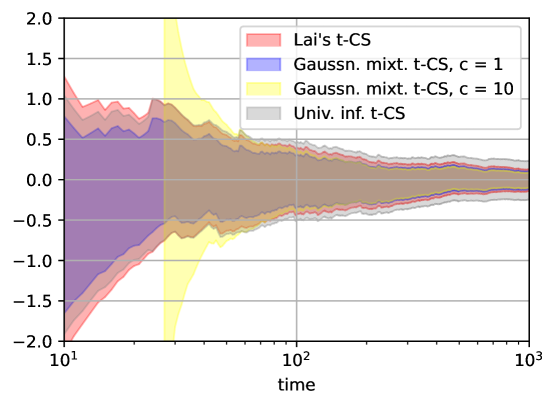
Figure 1: Three confidence sequences for t-test under $N_{0,1}$ observations.

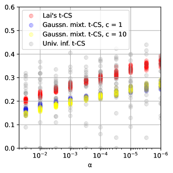
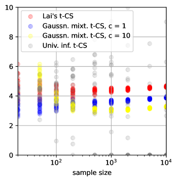
Figure 2: The rate of growth (left) at $n=500$ and rate of shrinkage (right) at $\alpha=0.05$ of the widths of three confidence sequences. In the left plot, the $y$-axis is widths whereas in the right plot, the $y$-axis is widths multiplied by $\sqrt{\text{sample size}}$ for clarity. Under $N_{0,1}$ observations, repeated 20 times.

First, we present them visually in the plot of Figure 1 in a single run of i.i.d. standard normal observations. We see that the Gaussian mixture CS we derived in Section 4.5 with $c=1$ performs better than Lai’s improper, flat mixture one; increasing $c$ results in interval explosion at earlier times but is slightly tighter at later times. The universal inference CS seems unfavorable at later times, but we shall soon see in repeated experiments that this is not necessarily the case.

We next compare their rates of growth and shrinkage. Still drawing observations from i.i.d. $N_{0,1}$, we first fix $n=500$ and let $\alpha$ vary, then fix $\alpha=0.05$ and let $n$ vary, plotting the widths of the CSs in 20 independent runs, since all of these CSs have random widths. The results are shown in Figure 2. We see with greater clarity that Lai’s CS is looser than Gaussian mixture-based CSs especially when $\alpha$ is small, even though the extended Ville’s inequality seems a tighter and more advanced technique; larger precision $c^{2}$ in Gaussian mixture gradually gains an advantage as $n$ increases. Even after a “smoothing” prior, the universal inference CS is still the most volatile. Its width varies a lot with different runs.

Acknowledgement

The authors acknowledge support from NSF grants IIS-2229881 and DMS-2310718.

Appendix A Omitted Proofs

Proof of Lemma 2.5.

Let $A\subseteq\mathbb{R}^{n-1}$ be measurable. Then,

$$\mathrm{E}_{\mathbbmsl P}\left(\mathbbmss{1}_{\{(X_{1},\dots,X_{n-1})\in A\}}\cdot\frac{\mathrm{d}\mathbbmsl Q_{(n-1)}}{\mathrm{d}\mathbbmsl P_{(n-1)}}(X_{1},\dots,X_{n-1})\right)$$ (45)

$$= \int_{A}\frac{\mathrm{d}\mathbbmsl Q_{(n-1)}}{\mathrm{d}\mathbbmsl P_{(n-1)}}(x_{1},\dots,x_{n-1})\,\mathrm{d}\mathbbmsl P_{(n-1)}(x_{1},\dots,x_{n-1})=\mathbbmsl Q_{(n-1)}(A).$$ (46)

And

$$\mathrm{E}_{\mathbbmsl P}\left(\mathbbmss{1}_{\{(X_{1},\dots,X_{n-1})\in A\}}\cdot\frac{\mathrm{d}\mathbbmsl Q_{(n)}}{\mathrm{d}\mathbbmsl P_{(n)}}(X_{1},\dots,X_{n})\right)$$ (47)

$$= \int_{A\times\mathbb{R}}\frac{\mathrm{d}\mathbbmsl Q_{(n)}}{\mathrm{d}\mathbbmsl P_{(n)}}(x_{1},\dots,x_{n})\,\mathrm{d}P_{n}(x_{1},\dots,x_{n})=\mathbbmsl Q_{(n)}(A\times\mathbb{R})=\mathbbmsl Q_{(n-1)}(A).$$ (48)

Since $A$ is arbitrary, we conclude that

$$\mathrm{E}_{\mathbbmsl P}\left(\frac{\mathrm{d}\mathbbmsl Q_{(n)}}{\mathrm{d}\mathbbmsl P_{(n)}}(X_{1},\dots,X_{n})\middle|X_{1},\dots,X_{n-1}\right)=\frac{\mathrm{d}\mathbbmsl Q_{(n-1)}}{\mathrm{d}\mathbbmsl P_{(n-1)}}(X_{1},\dots,X_{n-1}),$$ (49)

concluding the proof. ∎

Proof of Theorem 3.2.

For each $\sigma>0$ consider the likelihood ratio martingale under $\mathcal{N}(\mu,\sigma^{2})$

$$M_{n}^{\mu,\sigma^{2}}=\frac{\prod_{i=1}^{n}p_{\widetilde{\mu}_{i-1},\widetilde{\sigma}^{2}_{i-1}}(X_{i})}{\prod_{i=1}^{n}p_{\mu,\sigma^{2}}(X_{i})}.$$ (50)

The following process is an e-process under any $\mathcal{N}(\mu,\cdot)$

$$R_{n}^{\mu}=\frac{\prod_{i=1}^{n}p_{\widetilde{\mu}_{i-1},\widetilde{\sigma}^{2}_{i-1}}(X_{i})}{\sup_{s>0}\prod_{i=1}^{n}p_{\mu,s^{2}}(X_{i})}=\inf_{s>0}M_{n}^{\mu,s^{2}}.$$ (51)

Note that

$$\sup_{\sigma>0}\operatorname*{\mathbb{P}}_{\mathcal{N}(\mu,\sigma^{2})}[\exists n,R_{n}^{\mu}\geqslant 1/\alpha]\leqslant\operatorname*{\mathbb{P}}_{\mathcal{N}(\mu,\sigma^{2})}[\exists n,M_{n}^{\mu,\sigma^{2}}\geqslant 1/\alpha]\leqslant\alpha.$$ (52)

Since $s=\sqrt{\frac{\sum(X_{i}-\mu)^{2}}{n}}$ maximizes the denominator of $R_{n}^{\mu}$, it has a closed-form expression:

$$R_{n}^{\mu}=\frac{\prod\frac{1}{\widetilde{\sigma}_{i-1}}\exp\left\{-\frac{1}{2}\left(\frac{X_{i}-\widetilde{\mu}_{i-1}}{\widetilde{\sigma}_{i-1}}\right)^{2}\right\}}{\sup_{s>0}\prod\frac{1}{s}\exp\left\{-\frac{1}{2}\left(\frac{X_{i}-\mu}{s}\right)^{2}\right\}}=\frac{\prod\frac{1}{\widetilde{\sigma}_{i-1}}\exp\left\{-\frac{1}{2}\left(\frac{X_{i}-\widetilde{\mu}_{i-1}}{\widetilde{\sigma}_{i-1}}\right)^{2}\right\}}{\left(\frac{\sum(X_{i}-\mu)^{2}}{n}\right)^{-n/2}\exp\left\{-\frac{n}{2}\right\}}.$$ (53)

Hence due to (52), with probability at least $1-\alpha$, for all $n$,

$$\frac{\sum(X_{i}-\mu)^{2}}{n}\leqslant \left\{\ \frac{1}{\alpha}\exp\left\{-\frac{n}{2}\right\}\prod{\widetilde{\sigma}_{i-1}}\exp\left\{\frac{1}{2}\left(\frac{X_{i}-\widetilde{\mu}_{i-1}}{\widetilde{\sigma}_{i-1}}\right)^{2}\right\}\ \right\}^{2/n}$$ (54)

$$= \frac{1}{\alpha^{2/n}\mathrm{e}}\prod_{i=1}^{n}{\widetilde{\sigma}_{i-1}^{2/n}}\exp\left\{\frac{1}{n}\left(\frac{X_{i}-\widetilde{\mu}_{i-1}}{\widetilde{\sigma}_{i-1}}\right)^{2}\right\}$$ (55)

$$= \underbrace{\frac{1}{\alpha^{2/n}\mathrm{e}}\exp\left\{\frac{\sum_{i=1}^{n}\log\widetilde{\sigma}_{i-1}^{2}+\left(\frac{X_{i}-\widetilde{\mu}_{i-1}}{\widetilde{\sigma}_{i-1}}\right)^{2}}{n}\right\}}_{T_{n}}$$ (56)

Recall that the random variable on the RHS is $T_{n}$. The UI-CS then reads

$$\operatorname{CI}_{n}=\left[\widehat{\mu}_{n}\pm\sqrt{\widehat{\mu}_{n}^{2}-\overline{X^{2}_{n}}+T_{n}}\right].$$ (57)

∎

Prood of Proposition 3.3.

Note that

$$\frac{1}{n}\log R_{n}=\frac{1}{2}\log{\overline{X^{2}_{n}}}+\frac{1}{2}-\frac{\sum_{i=1}^{n}\log\widetilde{\sigma}_{i-1}}{n}-\frac{\sum_{i=1}^{n}\left(\frac{X_{i}-\widetilde{\mu}_{i-1}}{\widetilde{\sigma}_{i-1}}\right)^{2}}{2n}.$$ (58)

The first three terms converge a.s. to $\frac{1}{2}\log(\mu^{2}+\sigma^{2})$, $1/2$, and $\log\sigma$. It remains to show that the last term above converges a.s. to $1/2$.

Define $A_{n}=\sum_{i=1}^{n}\frac{1}{i}\left|\left(\frac{X_{i}-\mu}{\widetilde{\sigma}_{i-1}}\right)^{2}-\left(\frac{X_{i}-\mu}{\sigma}\right)^{2}\right|$. Then,

$$\mathrm{E}_{P}(A_{n})=\sum_{i=1}^{n}\frac{1}{i}\mathrm{E}_{P}\left(|X_{i}-\mu|^{2}\cdot|\widetilde{\sigma}_{i-1}^{-2}-\sigma^{-2}|\right)$$ (59)

$$\leqslant \sum_{i=1}^{n}\frac{1}{i}\mathrm{E}_{P}\left(\frac{(X_{i}-\mu)^{4}i^{-\gamma/2}+(\widetilde{\sigma}_{i-1}^{-2}-\sigma^{-2})^{2}i^{\gamma/2}}{2}\right)$$ (60)

$$= \frac{1}{2}\sum_{i=1}^{n}\frac{1}{i}\left(\mathrm{E}_{P}(X_{i}-\mu)^{4}\cdot i^{-\gamma/2}+\mathrm{E}_{P}(\widetilde{\sigma}_{i-1}^{-2}-\sigma^{-2})^{2}\cdot i^{\gamma/2}\right)$$ (61)

$$= \frac{1}{2}\sum_{i=1}^{n}\frac{1}{i}(\mathcal{O}(1)\cdot i^{-\gamma/2}+\mathcal{O}(i^{-\gamma})\cdot i^{\gamma/2})=\frac{1}{2}\sum_{i=1}^{n}\mathcal{O}(i^{-1-\gamma/2})=\mathcal{O}(1).$$ (62)

So there exists a constant $K>0$ such that $\mathrm{E}_{P}(A_{n})\leqslant K$ for all $n$. By Markov’s inequality and Fatou’s lemma,

$$P(\lim_{n\to\infty}A_{n}\geqslant a)\leqslant\frac{\mathrm{E}_{P}(\lim_{n\to\infty}A_{n})}{a}\leqslant\frac{\liminf_{n\to\infty}\mathrm{E}_{P}(A_{n})}{a}\leqslant\frac{K}{a},$$ (63)

which implies $P(\lim_{n\to\infty}A_{n}<\infty)=1$. By Kronecker’s lemma, this implies that

$$\lim_{n\to\infty}\frac{\sum_{i=1}^{n}\left\{\left(\frac{X_{i}-\mu}{\widetilde{\sigma}_{i-1}}\right)^{2}-\left(\frac{X_{i}-\mu}{\sigma}\right)^{2}\right\}}{n}=0\quad\text{almost surely.}$$ (64)

We now define $B_{n}=\sum_{i=1}^{n}\frac{1}{i}\left|\left(\frac{X_{i}-\widetilde{\mu}_{i-1}}{\widetilde{\sigma}_{i-1}}\right)^{2}-\left(\frac{X_{i}-\mu}{\widetilde{\sigma}_{i-1}}\right)^{2}\right|$. Without loss of generality assume $\sup_{n\geqslant 0}\mathrm{E}_{P}(\widetilde{\sigma}_{n}^{-6})<\infty$ (otherwise, if only $\sup_{n\geqslant n_{0}}\mathrm{E}_{P}(\widetilde{\sigma}_{n}^{-6})<\infty$ holds, use summation $\sum_{i=n_{0}+1}^{n}$ instead). Then,

$$\mathrm{E}_{P}(B_{n})=\sum_{i=1}^{n}\frac{1}{i}\mathrm{E}_{P}\left(\widetilde{\sigma}^{-2}_{i-1}\cdot|2X_{i}-\widetilde{\mu}_{i-1}-\mu|\cdot|\widetilde{\mu}_{i-1}-\mu_{1}|\right)$$ (65)

$$\leqslant\sum_{i=1}^{n}\frac{1}{i}\mathrm{E}_{P}\left(\frac{\widetilde{\sigma}^{-6}_{i-1}i^{-\gamma/4}+|2X_{i}-\widetilde{\mu}_{i-1}-\mu|^{3}i^{-\gamma/4}+|\widetilde{\mu}_{i-1}-\mu|^{3}i^{\gamma/2}}{3}\right)$$ (66)

$$=\frac{1}{3}\sum_{i=1}^{n}\frac{1}{i}\left(\mathrm{E}_{P}(\widetilde{\sigma}^{-6}_{i-1})\cdot i^{-\gamma/4}+\mathrm{E}_{P}(|2X_{i}-\widetilde{\mu}_{i-1}-\mu|^{3})\cdot i^{-\gamma/4}+\mathrm{E}_{P}(|\widetilde{\mu}_{i-1}-\mu|^{3})\cdot i^{\gamma/2}\right)$$ (67)

$$=\frac{1}{3}\sum_{i=1}^{n}\frac{1}{i}\left(\mathcal{O}(1)\cdot i^{-\gamma/4}+\mathcal{O}(1)\cdot i^{-\gamma/4}+\mathcal{O}(i^{-\gamma})\cdot i^{\gamma/2}\right)=\frac{1}{3}\sum_{i=1}^{n}\mathcal{O}(i^{-1-\gamma/4})=\mathcal{O}(1).$$ (68)

Similarly by Markov’s inequality, Fatou’s and Kronecker’s lemma,

$$\lim_{n\to\infty}\frac{\sum_{i=1}^{n}\left\{\left(\frac{X_{i}-\widetilde{\mu}_{i-1}}{\widetilde{\sigma}_{i-1}}\right)^{2}-\left(\frac{X_{i}-\mu}{\widetilde{\sigma}_{i-1}}\right)^{2}\right\}}{n}=0\quad\text{almost surely.}$$ (69)

Finally, strong law of large numbers implies that

$$\lim_{n\to\infty}\frac{\sum_{i=1}^{n}\left(\frac{X_{i}-\mu}{\sigma}\right)^{2}}{n}=1\quad\text{almost surely.}$$ (70)

Combining (64), (69), and (70), we see that

$$\lim_{n\to\infty}\frac{\sum_{i=1}^{n}\left(\frac{X_{i}-\widetilde{\mu}_{i-1}}{\widetilde{\sigma}_{i-1}}\right)^{2}}{n}=1\quad\text{almost surely.}$$ (71)

This concludes the proof. ∎

Proof of Theorem 3.4.

The following process is an e-process under any $\mathcal{N}(\mu,\sigma^{2})$, ($\mu\leqslant 0$ and $\sigma>0$).

$$\frac{\prod_{i=1}^{n}p_{\widetilde{\mu}_{i-1},\widetilde{\sigma}^{2}_{i-1}}(X_{i})}{\sup_{\begin{subarray}{c}m\leqslant 0\\ s>0\end{subarray}}\prod_{i=1}^{n}p_{m,s^{2}}(X_{i})}=\inf_{\begin{subarray}{c}m\leqslant 0\\ s>0\end{subarray}}M_{n}^{m,s^{2}}.$$ (72)

We have

$$\frac{\prod\frac{1}{\widetilde{\sigma}_{i-1}}\exp\left\{-\frac{1}{2}\left(\frac{X_{i}-\widetilde{\mu}_{i-1}}{\widetilde{\sigma}_{i-1}}\right)^{2}\right\}}{\sup_{m\leqslant 0}\sup_{s>0}\prod\frac{1}{s}\exp\left\{-\frac{1}{2}\left(\frac{X_{i}-m}{s}\right)^{2}\right\}}=\frac{\prod\frac{1}{\widetilde{\sigma}_{i-1}}\exp\left\{-\frac{1}{2}\left(\frac{X_{i}-\widetilde{\mu}_{i-1}}{\widetilde{\sigma}_{i-1}}\right)^{2}\right\}}{\sup_{m\leqslant 0}\left(\frac{\sum(X_{i}-m)^{2}}{n}\right)^{-n/2}\exp\left\{-\frac{n}{2}\right\}}$$ (73)

$$=\frac{\prod\frac{1}{\widetilde{\sigma}_{i-1}}\exp\left\{-\frac{1}{2}\left(\frac{X_{i}-\widetilde{\mu}_{i-1}}{\widetilde{\sigma}_{i-1}}\right)^{2}\right\}}{\sup_{m\leqslant 0}\left(m^{2}-2\widehat{\mu}_{n}m+\overline{X^{2}_{n}}\right)^{-n/2}\exp\left\{-\frac{n}{2}\right\}}$$ (74)

The denominator is maximized by $m=\widehat{\mu}_{n}\wedge 0$. Therefore

$$\dots= \frac{\prod\frac{1}{\widetilde{\sigma}_{i-1}}\exp\left\{-\frac{1}{2}\left(\frac{X_{i}-\widetilde{\mu}_{i-1}}{\widetilde{\sigma}_{i-1}}\right)^{2}\right\}}{\left((\widehat{\mu}_{n}\wedge 0-\widehat{\mu}_{n})^{2}+\overline{X^{2}_{n}}-\widehat{\mu}_{n}^{2}\right)^{-n/2}\exp\left\{-\frac{n}{2}\right\}}=\frac{\prod\frac{1}{\widetilde{\sigma}_{i-1}}\exp\left\{-\frac{1}{2}\left(\frac{X_{i}-\widetilde{\mu}_{i-1}}{\widetilde{\sigma}_{i-1}}\right)^{2}\right\}}{\left((0\vee\widehat{\mu}_{n})^{2}+\overline{X^{2}_{n}}-\widehat{\mu}_{n}^{2}\right)^{-n/2}\exp\left\{-\frac{n}{2}\right\}}$$ (75)

$$= \frac{\prod\frac{1}{\widetilde{\sigma}_{i-1}}\exp\left\{-\frac{1}{2}\left(\frac{X_{i}-\widetilde{\mu}_{i-1}}{\widetilde{\sigma}_{i-1}}\right)^{2}\right\}}{\left(\overline{X^{2}_{n}}-(\widehat{\mu}_{n}\wedge 0)^{2}\right)^{-n/2}\exp\left\{-\frac{n}{2}\right\}}=R_{n}^{-}.$$ (76)

∎

Proof of Proposition 3.5.

The four terms of

$$\frac{1}{n}\log R_{n}^{-}=\frac{1}{2}\log\left(\overline{X^{2}_{n}}-(\widehat{\mu}_{n}\wedge 0)^{2}\right)+\frac{1}{2}-\frac{\sum_{i=1}^{n}\log\widetilde{\sigma}_{i-1}}{n}-\frac{\sum_{i=1}^{n}\left(\frac{X_{i}-\widetilde{\mu}_{i-1}}{\widetilde{\sigma}_{i-1}}\right)^{2}}{2n}$$ (77)

converges a.s. to $\frac{1}{2}\log(\mu^{2}+\sigma^{2}-(\mu\wedge 0)^{2})$, $1/2$, $\log\sigma$, and $1/2$ respectively, concluding the proof. ∎

Proof of Lemma 4.4.

Let $Q^{+}_{n}$ be the distribution of $(X_{1},X_{2},\dots,X_{n})$ conditioned on $\{X_{1}>0\}$. Define the constant $p_{>0}=\mathbb{P}[X_{1}>0]=P_{\mu,\sigma}\{(0,\infty)\}$. Then,

$$\frac{\mathrm{d}Q^{+}_{n}}{\mathrm{d}\eta^{\otimes n}}(x_{1},x_{2},\dots,x_{n})=p_{>0}^{-1}\cdot\mathbbmss{1}(x_{1}>0)\cdot\prod_{i=1}^{n}\left\{\sigma^{-1}g(\sigma^{-1}(x_{i}-\mu))\right\},$$ (78)

meaning that for any measurable $A\subseteq\mathbb{R^{+}}\times\mathbb{R}^{n-1}$,

$$Q_{n}^{+}\{A\}=\int_{A}p_{>0}^{-1}\cdot\prod_{i=1}^{n}\left\{\sigma^{-1}g(\sigma^{-1}(x_{i}-\mu))\right\}\eta(\mathrm{d}x_{1})\eta(\mathrm{d}x_{2})\dots\eta(\mathrm{d}x_{n}).$$ (79)

Now recall $V_{n}:(x_{1},x_{2},\dots,x_{n})\mapsto(x_{1}/|x_{1}|,x_{2}/|x_{1}|,\dots,x_{n}/|x_{1}|)$. Let $Q_{n}^{*+}$ be the push-forward measure of $Q_{n}^{+}$ by $V_{n}$, a measure on $\{1\}\times\mathbb{R}^{n-1}$ (which is the conditional distribution of $(X_{1}/|X_{1}|,\dots,X_{n}/|X_{1}|)$ given $\{X_{1}>0\}$). Suppose the set $V_{n}(A)=\{1\}\times B$. We have the following change of variables (letting $(x_{1}^{*},\dots,x_{n}^{*})=V_{n}(x_{1},\dots,x_{n})$, so $x_{1}^{*}=1$ below),

$$Q_{n}^{*+}\{V_{n}(A)\}=Q_{n}^{+}\{A\}=\int_{A}p_{>0}^{-1}\cdot\prod_{i=1}^{n}\left\{\sigma^{-1}g(\sigma^{-1}(x_{i}-\mu))\right\}\eta(\mathrm{d}x_{1})\eta(\mathrm{d}x_{2})\dots\eta(\mathrm{d}x_{n})$$ (80)

$$=p_{>0}^{-1}\cdot\int_{x_{1}>0}\eta(\mathrm{d}x_{1})\int_{B}\prod_{i=1}^{n}\left\{\sigma^{-1}g(\sigma^{-1}(x_{i}^{*}|x_{1}|-\mu))\right\}\eta(\mathrm{d}x_{2}^{*})\dots\eta(\mathrm{d}x_{n}^{*})\left|\frac{\mathrm{d}(x_{2},\dots,x_{n})}{\mathrm{d}(x_{2}^{*},\dots,x_{n}^{*})}\right|$$ (81)

$$=p_{>0}^{-1}\cdot\int_{x_{1}>0}\eta(\mathrm{d}x_{1})\int_{B}\prod_{i=1}^{n}\left\{\sigma^{-1}g(\sigma^{-1}(x_{i}^{*}|x_{1}|-\mu))\right\}\eta(\mathrm{d}x_{2}^{*})\dots\eta(\mathrm{d}x_{n}^{*})\begin{vmatrix}\frac{1}{|x_{1}|}&0&\dots&0\\ 0&\frac{1}{|x_{1}|}&&0\\ \vdots&&\ddots&0\\ 0&\dots&0&\frac{1}{|x_{1}|}\end{vmatrix}^{-1}$$ (82)

$$=p_{>0}^{-1}\cdot\int_{x_{1}>0}\eta(\mathrm{d}x_{1})\int_{B}\prod_{i=1}^{n}\left\{\sigma^{-1}g(\sigma^{-1}(x_{i}^{*}x_{1}-\mu))\right\}x_{1}^{n-1}\eta(\mathrm{d}x_{2}^{*})\dots\eta(\mathrm{d}x_{n}^{*}).$$ (83)

We thus conclude that (letting $\delta_{1}$ be the Dirac point mass on 1),

$$\frac{\mathrm{d}Q_{n}^{*+}}{\delta_{1}\otimes\eta^{\otimes(n-1)}}(x_{1}^{*},x_{2}^{*},\dots,x_{n}^{*})=p_{>0}^{-1}\cdot\int_{x_{1}>0}\prod_{i=1}^{n}\left\{\sigma^{-1}g(\sigma^{-1}(x_{i}^{*}x_{1}-\mu))\right\}x_{1}^{n-1}\eta(\mathrm{d}x_{1}).$$ (84)

We can simplify the integral above by substituting $\tau=\sigma/x_{1}$, obtaining,

$$\frac{\mathrm{d}Q_{n}^{*+}}{\delta_{1}\otimes\eta^{\otimes(n-1)}}(x_{1}^{*},x_{2}^{*},\dots,x_{n}^{*})$$ (85)

$$= p_{>0}^{-1}\cdot\int_{\tau>0}\left\{\sigma^{-1}g(1/\tau-\sigma^{-1}\mu)\right\}\left\{\prod_{i=2}^{n}\sigma^{-1}g(x_{i}^{*}/\tau-\sigma^{-1}\mu))\right\}(\sigma/\tau)^{n-1}\sigma(1/\tau^{2})\eta(\mathrm{d}\tau)$$ (86)

$$= p_{>0}^{-1}\cdot\int_{\tau>0}\left\{\prod_{i=1}^{n}(1/\tau)g(x_{i}^{*}/\tau-\mu/\sigma))\right\}(1/\tau)\mathrm{d}\tau.$$ (87)

Similarly, let $Q_{n}^{*-}$ be the conditional distribution of $(X_{1}/|X_{1}|,\dots,X_{n}/|X_{1}|)$ given $\{X_{1}<0\}$). We have

$$\frac{\mathrm{d}Q_{n}^{*-}}{\delta_{-1}\otimes\eta^{\otimes(n-1)}}(x_{1}^{*},x_{2}^{*},\dots,x_{n}^{*})=(1-p_{>0})^{-1}\cdot\int_{\tau>0}\left\{\prod_{i=1}^{n}(1/\tau)g(x_{i}^{*}/\tau-\mu/\sigma))\right\}(1/\tau)\mathrm{d}\tau.$$ (88)

Finally, the measure $Q_{n}^{*}=\mathbbmss{1}_{\{x_{1}>0\}}\cdot p_{>0}\cdot Q_{n}^{*+}+\mathbbmss{1}_{\{x_{1}<0\}}\cdot(1-p_{>0})\cdot Q_{n}^{*-}$. So we see that

$$\frac{\mathrm{d}Q_{n}}{\mathrm{d}\eta^{\langle n-1\rangle}}(x_{1}^{*},\dots,x_{n}^{*})=\int_{\tau>0}\left\{\prod_{i=1}^{n}(1/\tau)g(x_{i}^{*}/\tau-\mu/\sigma))\right\}\frac{\mathrm{d}\tau}{\tau}$$ (89)

holds for both $x_{1}^{*}=\pm 1$. This concludes the proof. ∎

From now, let us denote

$$p^{*}_{\theta}(x_{1}^{*},\dots,x_{n}^{*})=\int_{\tau>0}\left\{\prod_{i=1}^{n}(1/\tau)g(x_{i}^{*}/\tau-\theta))\right\}(1/\tau)\mathrm{d}\tau,$$ (90)

i.e. the density $\frac{\mathrm{d}Q_{n}}{\mathrm{d}\eta^{\langle n-1\rangle}}$ when $P_{\mu,\sigma^{2}}$ satisfies $\mu/\sigma=\theta$. Here is a property of $p_{\theta}^{*}$.

Proposition A.1.

Let $\lambda>0$ be any constant. Then, $p^{*}_{\theta}(\lambda x_{1}^{*},\dots,\lambda x_{n}^{*})=\lambda^{-n}p^{*}_{\theta}(x_{1}^{*},\dots,x_{n}^{*})$. In particular, taking $\lambda=|x_{1}|$, we have $p^{*}_{\theta}(x_{1},\dots,x_{n})=|x_{1}|^{-n}p^{*}_{\theta}(x_{1}^{*},\dots,x_{n}^{*})$.

Proof of Proposition A.1.

$$p^{*}_{\theta}(\lambda x_{1}^{*},\dots,\lambda x_{n}^{*})$$ (91)

$$= \int_{\tau>0}\left\{\prod_{i=1}^{n}(1/\tau)g(\lambda x_{i}^{*}/\tau-\theta))\right\}(1/\tau)\mathrm{d}\tau$$ (92)

$$= \int_{\gamma=\lambda^{-1}\tau>0}\left\{\prod_{i=1}^{n}(1/\lambda\gamma)g(x_{i}^{*}/\gamma-\theta))\right\}(1/\lambda\gamma)\lambda\mathrm{d}\gamma$$ (93)

$$= \lambda^{-n}p^{*}_{\theta}(x_{1}^{*},\dots,x_{n}^{*}).$$ (94)

∎

Proof of Lemma 4.5.

Denote $X_{i}/|X_{1}|$ by $X_{i}^{*}$.

$$h_{n}(\theta;\theta_{0})=\underbrace{\frac{p^{*}_{\theta}(X_{1},\dots,X_{n})}{p_{\theta_{0}}^{*}(X_{1},\dots,X_{n})}=\frac{p^{*}_{\theta}(X_{1}^{*},\dots,X_{n}^{*})}{p_{\theta_{0}}^{*}(X_{1}^{*},\dots,X_{n}^{*})}}_{\text{equality due to \lx@cref{creftype~refnum}{lem:scaling}}}=\frac{\mathrm{d}Q^{n}_{\mu,\sigma^{2}}}{\mathrm{d}Q^{n}_{\mu_{0},\sigma^{2}_{0}}}(X_{1}^{*},\dots,X_{n}^{*}).$$ (95)

for any $\mu/\sigma=\theta$ and $\mu_{0}/\sigma_{0}=\theta_{0}$. Now it follows from Lemma 2.5 that $\{h_{n}(\theta;\theta_{0})\}$ is an NM for $P_{\mu_{0},\sigma^{2}_{0}}$ on the canonical filtration generated by $\{X_{n}^{*}\}$, which according to Proposition 4.3 is just $\{\mathcal{F}_{n}^{*}\}$. ∎

Proof of Corollary 4.6.

Using $g(x)=\frac{1}{\sqrt{2\pi}}\exp(-x^{2}/2)$ in (90),

$$p^{*}_{\theta}(x_{1},\dots,x_{n})=\int_{\tau>0}\left\{\prod_{i=1}^{n}(1/\tau)g(x_{i}/\tau-\theta))\right\}(1/\tau)\mathrm{d}\tau$$ (96)

$$= \frac{1}{(2\pi)^{n/2}}\int_{\tau>0}\left\{\prod_{i=1}^{n}\mathrm{e}^{-(x_{i}/\tau-\theta)^{2}/2}\right\}\frac{1}{\tau^{n+1}}\mathrm{d}\tau$$ (97)

$$= \frac{\mathrm{e}^{-n\theta^{2}/2}}{(2\pi)^{n/2}}\int_{\tau>0}\exp\left\{-\frac{\sum_{i=1}^{n}{x_{i}}^{2}}{2\tau^{2}}+\frac{\theta\sum_{i=1}^{n}x_{i}}{\tau}\right\}\frac{1}{\tau^{n+1}}\mathrm{d}\tau.$$ (98)

Therefore, applying Lemma 4.5 with $\theta_{0}=0$, we have

$$h_{n}(\theta;0)=\mathrm{e}^{-n\theta^{2}/2}\frac{\int_{\tau>0}\exp\left\{-\frac{\sum_{i=1}^{n}{X_{i}}^{2}}{2\tau^{2}}+\frac{\theta\sum_{i=1}^{n}X_{i}}{\tau}\right\}\frac{1}{\tau^{n+1}}\mathrm{d}\tau}{\int_{\tau>0}\exp\left\{-\frac{\sum_{i=1}^{n}{X_{i}}^{2}}{2\tau^{2}}\right\}\frac{1}{\tau^{n+1}}\mathrm{d}\tau}$$ (99)

(the denominator being a generalized Gaussian integral) (100)

$$= \frac{\mathrm{e}^{-n\theta^{2}/2}}{\Gamma(n/2)}\int_{y>0}y^{n/2-1}\exp\left\{-y+\theta\left(\sum_{i=1}^{n}X_{i}\right)\sqrt{\frac{2y}{\sum_{i=1}^{n}{X_{i}}^{2}}}\right\}\mathrm{d}y,$$ (101)

coinciding with $h_{\theta,n}$. ∎

Proof of Theorem 4.7 (as well as Theorem 4.1).

Putting a flat, improper prior $\mathrm{d}\pi(\theta)=\mathrm{d}\theta$ over $\mathbb{R}$, we have the following improperly mixed, extended nonnegative supermartingale,

$$H_{n}=\int h_{\theta,n}\pi(\mathrm{d}\theta)$$ (102)

$$= \int_{\theta}\frac{\mathrm{e}^{-n\theta^{2}/2}}{\Gamma(n/2)}\left(\int_{y>0}y^{n/2-1}\exp\left\{-y+\theta\left(\sum_{i=1}^{n}X_{i}\right)\sqrt{\frac{2y}{\sum_{i=1}^{n}{X_{i}}^{2}}}\right\}\mathrm{d}y\right)\cdot\mathrm{d}\theta$$ (103)

$$= \frac{1}{\Gamma(n/2)}\int_{y>0}y^{n/2-1}\mathrm{e}^{-y}\left(\int_{\theta}\exp\left\{-\frac{n}{2}\theta^{2}+\theta\left(\sum_{i=1}^{n}X_{i}\right)\sqrt{\frac{2y}{\sum_{i=1}^{n}{X_{i}}^{2}}}\right\}\mathrm{d}\theta\right)\mathrm{d}y$$ (104)

$$= \frac{1}{\Gamma(n/2)}\int_{y>0}y^{n/2-1}\mathrm{e}^{-y}\left(\sqrt{\frac{2\pi}{n}}\exp\left\{\frac{\left(\sum_{i=1}^{n}X_{i}\right)^{2}\frac{2y}{\sum_{i=1}^{n}{X_{i}}^{2}}}{2n}\right\}\right)\mathrm{d}y$$ (105)

$$= \frac{1}{\Gamma(n/2)}\sqrt{\frac{2\pi}{n}}\int_{y>0}y^{n/2-1}\exp\left\{-\left(1-\frac{S_{n}^{2}}{nV_{n}}\right)y\right\}\mathrm{d}y$$ (106)

$$= \frac{1}{\Gamma(n/2)}\sqrt{\frac{2\pi}{n}}\Gamma(n/2)\left(1-\frac{S_{n}^{2}}{nV_{n}}\right)^{-n/2}=\sqrt{\frac{2\pi}{n}}\left(1-\frac{S_{n}^{2}}{nV_{n}}\right)^{-n/2}$$ (107)

$$= \sqrt{\frac{2\pi}{n}}\left(\frac{nV_{n}}{nV_{n}-S_{n}^{2}}\right)^{n/2}$$ (108)

Note that when $n=1$, $nV_{n}-S_{n}^{2}=0$, and $H_{0}$ is understood to be $+\infty$. Note that

$$t_{n-1}\sim\frac{\frac{1}{n}S_{n}}{\frac{1}{\sqrt{n}}\sqrt{\frac{1}{n-1}(V_{n}-\frac{1}{n}S_{n}^{2})}}=\sqrt{n-1}\sqrt{\frac{S_{n}^{2}}{nV_{n}-S_{n}^{2}}}=:T_{n-1}$$ (109)

Then $H_{n}=\sqrt{\frac{2\pi}{n}}\left(\frac{T_{n-1}^{2}}{n-1}+1\right)^{n/2}$.

In terms of CS, every $X_{i}$ should be seen as $X_{i}-0=X_{i}-\mu$, and hence

$$H_{n}^{\mu}=\sqrt{\frac{2\pi}{n}}\left(\frac{n\sum(X_{i}-\mu)^{2}}{n\sum(X_{i}-\mu)^{2}-(\sum(X_{i}-\mu))^{2}}\right)^{n/2}$$ (110)

is also an (improperly mixed) NSM.

The extended Ville’s inequality, applied on the process $\sqrt{m/2\pi}H_{n}^{\mu}$, reads,

With probability at most

$$P=\mathbb{P}\left[\frac{T_{m-1}^{2}}{m-1}+1\geqslant\eta\right]+\eta^{-m/2}\mathbb{E}\left[\mathbbmss{1}_{\left\{\frac{T_{m-1}^{2}}{m-1}+1<\eta\right\}}\left(\frac{T_{m-1}^{2}}{m-1}+1\right)^{m/2}\right],$$ (111)

there exists $n\geqslant m$,

$$\sqrt{\frac{m}{n}}\left(\frac{n\sum(X_{i}-\mu)^{2}}{n\sum(X_{i}-\mu)^{2}-(\sum(X_{i}-\mu))^{2}}\right)^{n/2}\geqslant\eta^{m/2}.$$ (112)

Define $a=\sqrt{(m-1)(\eta-1)}$. Then $\eta^{m/2}=(1+a^{2}/(m-1))^{m/2}=h(a)$ and

$$P =\mathbb{P}[|T_{m-1}|\geqslant a]+h(a)^{-1}\mathbb{E}[\mathbbmss{1}_{\{|T_{m-1}|<a\}}h(T_{m-1})]$$ (113)

$$=2\mathbb{P}[T_{m-1}>a]+2\frac{\mathbb{E}[\mathbbmss{1}_{\{0\leqslant T_{m-1}<a\}}h(T_{m-1})]}{h(a)}$$ (114)

Let $f_{m-1}$, $F_{m-1}$ be the density and CDF of $T_{m-1}$. The expectation $\mathbb{E}[\mathbbmss{1}_{\{0\leqslant T_{m-1}<a\}}h(T_{m-1})]$ must be smaller than $\frac{a}{a-a^{\prime}}\mathbb{E}[\mathbbmss{1}_{\{a^{\prime}\leqslant T_{m-1}<a\}}h(T_{m-1})]$, for all $a^{\prime}\in(0,a)$. Note that

$$\lim_{a^{\prime}\to a}\frac{a}{a-a^{\prime}}\mathbb{E}[\mathbbmss{1}_{\{a^{\prime}\leqslant T_{m-1}<a\}}h(T_{m-1})]=ah(a)f_{m-1}(a).$$ (115)

Hence

$$P\leqslant 2(1-F_{m-1}(a))+2af_{m-1}(a).$$ (116)

This concludes the missing proof of Lai CS. ∎

Proof of Theorem 4.9.

Let us put a Gaussian prior on $\theta$,

$$\frac{\mathrm{d}\pi(\theta)}{\mathrm{d}\theta}=\frac{c}{\sqrt{2\pi}}\mathrm{e}^{-c^{2}\theta^{2}/2},$$ (117)

and define the martingale

$$H_{n}=\int h_{\theta,n}\pi(\mathrm{d}\theta)$$ (118)

$$= \int_{\theta}\frac{\mathrm{e}^{-n\theta^{2}/2}}{\Gamma(n/2)}\left(\int_{y>0}y^{n/2-1}\exp\left\{-y+\theta\left(\sum_{i=1}^{n}X_{i}\right)\sqrt{\frac{2y}{\sum_{i=1}^{n}{X_{i}}^{2}}}\right\}\mathrm{d}y\right)\cdot\pi(\mathrm{d}\theta)$$ (119)

$$= \frac{c}{\sqrt{2\pi}\Gamma(n/2)}\int_{y>0}y^{n/2-1}\mathrm{e}^{-y}\left(\int_{\theta}\exp\left\{-\frac{n+c^{2}}{2}\theta^{2}+\theta\left(\sum_{i=1}^{n}X_{i}\right)\sqrt{\frac{2y}{\sum_{i=1}^{n}{X_{i}}^{2}}}\right\}\mathrm{d}\theta\right)\mathrm{d}y$$ (120)

$$= \frac{c}{\sqrt{2\pi}\Gamma(n/2)}\int_{y>0}y^{n/2-1}\mathrm{e}^{-y}\left(\sqrt{\frac{\pi}{\frac{n+c^{2}}{2}}}\exp\left\{\frac{\left(\sum_{i=1}^{n}X_{i}\right)^{2}\frac{2y}{\sum_{i=1}^{n}{X_{i}}^{2}}}{2(n+c^{2})}\right\}\right)\mathrm{d}y$$ (121)

$$= \frac{c}{\sqrt{2\pi}\Gamma(n/2)}\sqrt{\frac{\pi}{\frac{n+c^{2}}{2}}}\int_{y>0}y^{n/2-1}\exp\left\{-\left(1-\frac{S_{n}^{2}}{(n+c^{2})V_{n}}\right)y\right\}\mathrm{d}y$$ (122)

$$= \frac{c}{\Gamma(n/2)}\sqrt{\frac{1}{n+c^{2}}}\Gamma(n/2)\left(1-\frac{S_{n}^{2}}{(n+c^{2})V_{n}}\right)^{-n/2}=\sqrt{\frac{c^{2}}{n+c^{2}}}\left(1-\frac{S_{n}^{2}}{(n+c^{2})V_{n}}\right)^{-n/2}.$$ (123)

This is a valid test martingale.

While this is a test martingale for $\mathcal{N}_{\mu=0}$, a shifting argument ($X_{i}\to X_{i}-\mu_{0}$) yields that

$$H_{n}^{\mu_{0}}=\sqrt{\frac{c^{2}}{n+c^{2}}}\left(1-\frac{(S_{n}-n\mu_{0})^{2}}{(n+c^{2})(V_{n}-2S_{n}\mu_{0}+n\mu_{0}^{2})}\right)^{-n/2}$$ (124)

is a test martingale for $\mathcal{N}_{\mu=\mu_{0}}$. Applying Ville’s inequality, with probability at least $1-\alpha$, for all $n$,

$$\frac{nc^{2}\mu_{0}^{2}-2c^{2}S_{n}\mu_{0}+(n+c^{2})V_{n}-S_{n}^{2}}{(n+c^{2})(n\mu_{0}^{2}-2S_{n}\mu_{0}+V_{n})} \geqslant\left(\frac{\alpha^{2}c^{2}}{n+c^{2}}\right)^{1/n},$$ (125)

$$\frac{nc^{2}(\mu_{0}-\widehat{\mu}_{n})^{2}+(n+c^{2})(V_{n}-S_{n}^{2}/n)}{(n+c^{2})(n(\mu_{0}-\widehat{\mu}_{n})^{2}+V_{n}-S_{n}^{2}/n)} \geqslant\left(\frac{\alpha^{2}c^{2}}{n+c^{2}}\right)^{1/n},$$ (126)

$$\left\{\left(\frac{\alpha^{2}c^{2}}{n+c^{2}}\right)^{1/n}(n+c^{2})n-nc^{2}\right\}(\mu_{0}-\widehat{\mu}_{n})^{2} \leqslant\left\{(n+c^{2})\left(1-\left(\frac{\alpha^{2}c^{2}}{n+c^{2}}\right)^{1/n}\right)\right\}(V_{n}-S_{n}^{2}/n),$$ (127)

$$(\mu_{0}-\widehat{\mu}_{n})^{2} \leqslant\frac{(n+c^{2})\left(1-\left(\frac{\alpha^{2}c^{2}}{n+c^{2}}\right)^{1/n}\right)}{\left(\frac{\alpha^{2}c^{2}}{n+c^{2}}\right)^{1/n}(n+c^{2})-c^{2}}\left(\overline{X^{2}_{n}}-\widehat{\mu}_{n}^{2}\right)$$ (128)

This concludes the proof ∎

Proof of Proposition 4.8.

First, under $N_{\mu,\sigma^{2}}$, note that $T_{n-1}=\sqrt{n-1}\frac{S_{n}-n\mu}{\sqrt{nV_{n}-S_{n}^{2}}}$ and $v_{n}=V_{n}/n-S_{n}^{2}/n^{2}$. We replace $\frac{T_{n-1}}{\sqrt{n-1}}$ by $\frac{T_{n-1}}{\sqrt{n-1}}+\frac{\mu_{1}}{\sqrt{v_{n}}}$ in (33) to have

$$H_{n}=\sqrt{\frac{2\pi}{n}}\left(1+\left(\frac{T_{n-1}}{\sqrt{n-1}}+\frac{\mu}{\sqrt{v_{n}}}\right)^{2}\right)^{n/2},$$ (129)

$$\frac{\log H_{n}}{n}=\frac{\log(2\pi/n)}{2n}+\frac{1}{2}\log\left(1+\left(\frac{T_{n-1}}{\sqrt{n-1}}+\frac{\mu}{\sqrt{v_{n}}}\right)^{2}\right).$$ (130)

It is well known $v_{n}$ converges to $\sigma^{2}$ almost surely. Therefore $\frac{T_{n-1}}{\sqrt{n-1}}=\frac{\widehat{\mu}_{n}-\mu_{1}}{\sqrt{v_{n}}}$ converges almost surely to 0. These imply that $\frac{\log H_{n}}{n}$ converges almost surely to $\frac{1}{2}\log(1+\mu^{2}/\sigma^{2})$.

Second, under any $P\in\mathcal{N}_{\mu=0}$, let $\delta>0$. By (33) we have

$$P(H_{n}>\delta)=P\Bigg{(}T_{n-1}^{2}>\underbrace{\left(\left(\frac{\delta^{2}n}{2\pi}\right)^{1/n}-1\right)(n-1)}_{\gtrsim\log n}\Bigg{)}\lesssim P(T_{1}^{2}>\log n).$$ (131)

The underbraced term grows logarithmically because $n^{1/n}-1=\frac{\log n}{n}+\mathcal{O}(n^{-2})$. The “$\lesssim$” holds because the tail of Student’s t-distribution strictly decreases when the DOF increases. So $P(H_{n}>\delta)$ goes to 0 as $n\to\infty$, concluding that $\{H_{n}\}$ converges to 0 in probability. By Wang and Ramdas [2023a, Proposition A.14], an ENSM converges almost surely, so $\{H_{n}\}$ converges to 0 almost surely. The proof is complete. ∎

Proof of Proposition 4.10.

First, under $N_{\mu,\sigma^{2}}$, we replace in (39) $\frac{T_{n-1}}{\sqrt{n-1}}$ by $\frac{T_{n-1}}{\sqrt{n-1}}+\frac{\mu}{\sqrt{v_{n}}}$,

$$G_{n}^{(c)}=\sqrt{\frac{c^{2}}{n+c^{2}}}\left(1+\frac{n}{\frac{n+c^{2}}{\left(\frac{T_{n-1}}{\sqrt{n-1}}+\frac{\mu}{\sqrt{v_{n}}}\right)^{2}}+{c^{2}}}\right)^{n/2},$$ (132)

$$\frac{\log G_{n}^{(c)}}{n}=\frac{\log(\frac{c^{2}}{n+c^{2}})}{2n}+\frac{1}{2}\log\left(1+\frac{n}{\frac{n+c^{2}}{\left(\frac{T_{n-1}}{\sqrt{n-1}}+\frac{\mu}{\sqrt{v_{n}}}\right)^{2}}+{c^{2}}}\right).$$ (133)

As in the proof of Proposition 4.8, $\frac{T_{n-1}}{\sqrt{n-1}}$ converges to 0 and $v_{n}$ to $\sigma^{2}$ almost surely. Therefore $\frac{\log G_{n}^{(c)}}{n}$ converges a.s. to $\frac{1}{2}\log(1+\mu^{2}/\sigma^{2})$.

Second, under any $P\in\mathcal{N}_{\mu=0}$, let $\delta>0$. By (39) we have

$$P(G_{n}^{(c)}>\delta)=P\Bigg{(}\frac{n}{\frac{(n+c^{2})(n-1)}{T_{n-1}^{2}}+{c^{2}}}>\underbrace{\left(\frac{(n+c^{2})\delta^{2}}{c^{2}}\right)^{1/n}-1}_{\gtrsim\frac{\log n}{n}}\Bigg{)}\lesssim P(T_{1}^{2}>\log n),$$ (134)

which converges to 0. So $\{G_{n}^{(c)}\}$ converges to 0 in probability. It thus also converges to 0 almost surely due to Doob’s martingale convergence theorem, concluding the proof. ∎

References

• Darling and Robbins [1967] D. A. Darling and H. Robbins. Confidence sequences for mean, variance, and median. Proceedings of the National Academy of Sciences, 58(1):66–68, 1967.
• Ghosh [1960] J. Ghosh. On some properties of sequential t-test. Calcutta Statistical Association Bulletin, 9(3):77–86, 1960.
• Grünwald et al. [2023] P. Grünwald, R. de Heide, and W. M. Koolen. Safe testing. Journal of the Royal Statistical Society: Series B (to appear with discussion), 2023.
• Hoel [1954] P. G. Hoel. On a property of the sequential t-test. Scandinavian Actuarial Journal, 1954(1):19–22, 1954.
• Howard et al. [2021] S. R. Howard, A. Ramdas, J. McAuliffe, and J. Sekhon. Time-uniform, nonparametric, nonasymptotic confidence sequences. The Annals of Statistics, 49(2):1055–1080, 2021.
• Johari et al. [2022] R. Johari, P. Koomen, L. Pekelis, and D. Walsh. Always valid inference: Continuous monitoring of A/B tests. Operations Research, 70(3):1806–1821, 2022.
• Klenke [2013] A. Klenke. Probability theory: a comprehensive course. Springer Science & Business Media, 2013.
• Lai [1976] T. L. Lai. On confidence sequences. The Annals of Statistics, pages 265–280, 1976.
• Pérez-Ortiz et al. [2022] M. F. Pérez-Ortiz, T. Lardy, R. de Heide, and P. Grünwald. E-statistics, group invariance and anytime valid testing. arXiv preprint arXiv:2208.07610, 2022.
• Ramdas et al. [2022] A. Ramdas, J. Ruf, M. Larsson, and W. M. Koolen. Testing exchangeability: Fork-convexity, supermartingales and e-processes. International Journal of Approximate Reasoning, 141:83–109, 2022.
• Robbins [1970] H. Robbins. Statistical methods related to the law of the iterated logarithm. The Annals of Mathematical Statistics, 41(5):1397–1409, 1970.
• Rouder et al. [2009] J. N. Rouder, P. L. Speckman, D. Sun, R. D. Morey, and G. Iverson. Bayesian t tests for accepting and rejecting the null hypothesis. Psychonomic bulletin & review, 16:225–237, 2009.
• Ruf et al. [2023] J. Ruf, M. Larsson, W. M. Koolen, and A. Ramdas. A composite generalization of Ville’s martingale theorem. Electronic Journal of Probability, 2023.
• Rushton [1950] S. Rushton. On a sequential t-test. Biometrika, 37(3/4):326–333, 1950.
• Sacks [1965] J. Sacks. A note on the sequential t-test. The Annals of Mathematical Statistics, 36(6):1867–1869, 1965.
• Student [1908] Student. The probable error of a mean. Biometrika, pages 1–25, 1908.
• Ville [1939] J. Ville. Etude critique de la notion de collectif. Bull. Amer. Math. Soc, 45(11):824, 1939.
• Wald [1945] A. Wald. Sequential tests of statistical hypotheses. The Annals of Mathematical Statistics, 16(2):117–186, 1945.
• Wald [1947] A. Wald. Sequential analysis. 1947.
• Wang and Ramdas [2023a] H. Wang and A. Ramdas. The extended Ville’s inequality for nonintegrable nonnegative supermartingales. arXiv preprint arXiv:2304.01163, 2023a.
• Wang and Ramdas [2023b] H. Wang and A. Ramdas. Catoni-style confidence sequences for heavy-tailed mean estimation. Stochastic Processes and their Applications, 163:168–202, 2023b.
• Wasserman et al. [2020] L. Wasserman, A. Ramdas, and S. Balakrishnan. Universal inference. Proceedings of the National Academy of Sciences, 117(29):16880–16890, 2020.
• Waudby-Smith and Ramdas [2023] I. Waudby-Smith and A. Ramdas. Estimating means of bounded random variables by betting. Journal of the Royal Statistical Society: Series B (Methodological), to appear with discussion, 2023.
• Zellner and Siow [1980] A. Zellner and A. Siow. Posterior odds ratios for selected regression hypotheses. Trabajos de estadística y de investigación operativa, 31:585–603, 1980.