Hadronic processes at work in 5BZB J0630$-$2406

Abstract

Recent observations are shedding light on the important role that active galactic nuclei (AGN) play in the production of high-energy neutrinos. In this study, we focus on one object, 5BZB J0630$-$2406, which is among the blazars recently proposed as associated with neutrino emission during the first $7$-yr IceCube observations. Modelling the quasi-simultaneous, broad-band spectral energy distribution, we explore various scenarios from purely leptonic to lepto-hadronic models, testing the inclusion of external photon fields. This theoretical study provides a complementary testing ground for the proposed neutrino-blazar association. Despite being historically classified as a BL Lac, our study shows that 5BZB J0630$-$2406 belongs to the relatively rare sub-class of high-power flat-spectrum radio quasars (FSRQs). Our results indicate that interactions between protons and external radiation fields can produce a neutrino flux that is within the reach of the IceCube detector. Furthermore, the spectral shape of the X-ray emission suggests the imprint of hadronic processes related to very energetic protons.

1 Introduction

Active galactic nuclei (AGN) are among the most energetic and powerful objects in the universe. They are powered by a supermassive black hole (SMBH), in some of them a relativistic jet can be present and detected across the electromagnetic spectrum, from the radio to the very high energy (VHE) band. Efficient particle acceleration mechanisms such as magnetic reconnection (Blandford et al. 2017) and shock acceleration (Pelletier et al. 2019; Lemoine et al. 2019) can occur in distinct regions of the jet. Standing and moving features observed in AGN jets (Marshall et al. 2002; Jorstad et al. 2013; Lister et al. 2021), also reproduced numerically as shocks (Fromm et al. 2016; Fichet de Clairfontaine et al. 2021, 2022), support the idea that the observed multi-wavelength (MWL) electromagnetic emission can be explained trough radiative cooling of those accelerated particles along the jet. While to date the overwhelming majority of AGN can be explained invoking the leptonic framework, from the theoretical point of view relativistic jets harbored in AGN may be capable of accelerating hadrons. Within such scenarios, high-energy (HE; TeV/PeV energies) neutrinos are a natural by-product.

Located at the geographic South Pole, the IceCube observatory is the most sensitive high-energy ($\gtrsim$ TeV) neutrino detector currently operating. Since the beginning of its science operations in $2008$, it allows us to study the putative neutrino counterparts of astrophysical sources. Although no firm associations between individual high-energy IceCube events and cosmic sources have been established to date, several claims of associations with AGN have been made at different statistical levels, e.g. the blazar TXS 0506$+$56, IceCube Collaboration et al. (2018a, b), which represent a subclass of AGN with the jet pointed directly at the observer.

Other approaches to studying such correlations exploit the time-integrated neutrino information over a given period of time, as in the case of observational evidence of neutrino emission in the direction of the Seyfert galaxy NGC 1068 (IceCube Collaboration et al. 2022), or through stacking analyses of populations of sources (e.g. Aartsen et al. 2017a; Padovani et al. 2016; Aartsen et al. 2017b; Abbasi et al. 2021; Plavin et al. 2021; Abbasi et al. 2023).

A recent work reports evidence for a statistically significant correlation between blazars listed in the fifth data release of the Roma-BZCat catalog (5BZCat, see Massaro et al. 2015), and a sample of IceCube hotspots, i.e. anisotropies in the distribution of IceCube events (Buson et al. 2022a, b). The study is based on the $7$-yr IceCube southern sky map published by the IceCube collaboration and highlights $10$ objects as candidate HE neutrino emitters, i.e. PeVatron blazars. Consistent findings are reported when expanding the investigation to the Northern Hemisphere with the latest sky map released by the IceCube collaboration (Buson et al. 2023). Investigations employing different analysis methodologies have provided mixed results. For instance, Bellenghi et al. (2023) performed an independent analysis of the public IceCube dataset, confirming the association established by Buson et al. (2022a, b) with the $7$-yr Southern Hemisphere dataset. However, when analyzing the $10$-year dataset, they did not observe a similar correlation. Such $10$-yr sky map appears overall different from the one published by IceCube collaboration with the same dataset (Aartsen et al. 2020), and the one used by (Buson et al. 2023) for the $10$-yr Northern Hemisphere analysis. The discrepancies can be attributed to the different likelihood formalism and the coarseness of the detector response matrices employed, that lead to an overall worst sensitivity, as acknowledged in Bellenghi et al. (2023).

Given the unascertained electromagnetic / neutrino relation, the statistical analysis was based solely on the positions of the objects. No a-priori selection was applied to the blazar sample, neither based on the objects’ classification nor on their electromagnetic properties.

This paper aims to provide an initial characterization of the underlying physics of PeVatron blazars from the theoretical perspective (Fichet de Clairfontaine et al. 2023). To this extent, we focus on one object for which broad, MWL simultaneous observations are available, namely 5BZB J0630$-$2406 (a.k.a. TXS 0628$-$240, WISE J063059.51$-$240646.2), while future works will address the physical properties of the sample (Azzollini et al. 2023).

Although the redshift of the source is unknown due to the lack of emission lines in the optical spectrum, a lower limit has been established $z\geq 1.239$ (Shaw et al. 2013), and absorption lines have been observed (Mg I, Fe II, Al II) that indicate the presence of the host galaxy (Rau et al. 2012a).

Theoretical modeling of the MWL emission of candidate neutrino emitters have shown the key role of external fields in the neutrino production (Dermer et al. 2014; Oikonomou et al. 2019) and markers of hadronic processes imprinted in the observed electromagnetic spectral energy distribution(SED, Reimer et al. 2019; Cerruti et al. 2018; Gao et al. 2019; Petropoulou et al. 2020; Rodrigues et al. 2021). Here, we model the SED of the object of interest, exploiting simultaneous and quasi-simultaneous MWL observations.

The paper is organized as follows. Sect. 2 introduces the neutrino observations that provided evidence of neutrino emission in the direction of 5BZB J0630$-$2406. The Sect. 3 displays the MWL observations and data reduction. The Sect. 4 discusses the temporal variability of this source. We present our approach to reproduce the observed SED with a one-zone leptonic and lepto-hadronic numerical models, with a complete description in Sect. 5. Then, in Sect. 6, we present the results of our parameter space exploration in different scenarios, including scenarios where the X-ray band is dominated by either synchrotron radiation or by hadronic cascade processes related to secondaries particles. The characteristics of the source derived from the various scenarios will be detailed, as well as the expected neutrino event rates. In Sect. 7, we discuss our findings and their implications in the context of recent neutrino - blazar associations.
Throughout the paper, all primed quantities are evaluated in the rest frame of the relativistic jet. We also assume a flat $\Lambda$CDM cosmology with $\rm{H}_{\rm 0}=69.6~{}\rm{km}\cdot\rm{s}^{-1}\cdot\rm{Mpc}^{-1}$, $\Omega_{\rm 0}=0.29$ and $\Omega_{\Lambda}=0.71$.

2 Neutrino observations

5BZB J0630$-$2406 has been proposed as candidate counterpart of the IceCube hotspot IC J0630$-$2353 (Buson et al. 2022a). The study presented in Buson et al. (2022a) is based on a Southern Hemisphere analysis ($\delta<-5$) of the all-sky map that spans the IceCube observations from $2008$ to June $2015$. This $7$-yr sky map encodes the time-integrated information regarding long-term point-source neutrino emitters and is built using events of energy-proxy $\gtrsim 100$ TeV. In the $7$-yr sky map, the direction of the IceCube hotspot IC J0630$-$2353 evidences an anisotropy in the spatial distribution of events (see Fig. 1) and, thus, may hint for the presence of astrophysical sources. The object is located at an angular separation of $0.28\degree$ from the hotspot IC J0630$-$2353, within the association radius of $0.55\degree$ derived for this dataset in Buson et al. (2022a). The evidence for a spatial correlation between IC J0630$-$2353 and the blazar 5BZB J0630$-$2406 suggests that this blazar may contribute to the observed anisotropy.

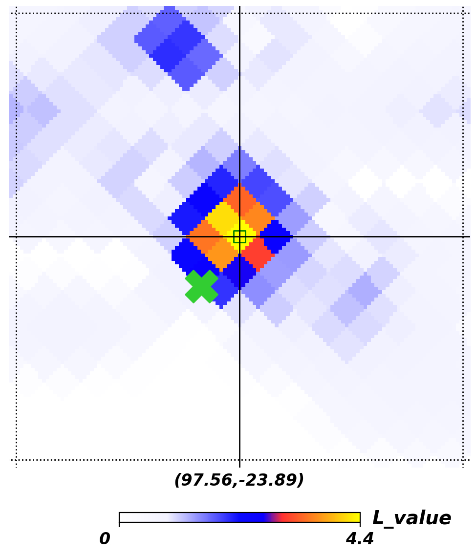
Figure 1: Cut-out region of the $7$-yr IceCube $L$-value map (Aartsen et al. 2017c) centered at the position of the hotspot IC J0630$-$2353, displayed in celestial coordinates. The position of the associated blazar 5BZB J0630$-$2406 is highlighted by a green cross. The black lines indicate the $1$ degree $\times$ $1$ degree coordinate grid.

3 Multiwavelength observations and data analysis

In the following, we provide a description of the MWL data collection and reduction. In Figure 2, we present the MWL light curves, from near-infrared (NIR) to $\gamma$ rays. The orange vertical line denotes the epoch of the simultaneous observations, used in the SED modeling presented in Sect. 5.

3.1 Radio observations

Archival radio data are available from the Academy of Sciences Radio Telescope (RATAN) , the GaLactic and Extragalactic All-sky Murchison Widefield Array (GLEAM, Hurley-Walker et al. (2017)) and the Australia Telescope 20-GHz (AT20G, Mahony et al. (2011)) catalog. They are not used in the modeling and rather considered as upper limits for the fit. At such lower frequencies, the radio flux is likely originated from extended regions of the jet, as the electrons cool down via low-energy synchrotron over a long period of time while propagated through the jet.

3.2 Near-infrared observations

NIR, aperture photometry (JHK) observations were obtained by the Gamma-Ray Burst Optical and Near-Infrared Detector (GROND) on $2010$–$09$–$28$ $08$:$06$ (MJD $55467$, Rau et al. 2012b) and $2014$–$10$–$19$ $05$:$29$ (MJD $56949$). The data were reduced and analyzed as explained in Ackermann et al. (2016).

3.3 Optical observations

Over the past decade 5BZB J0630$-$2406 has been monitored at optical wavelengths by several programs. The Katzman Automatic Imaging Telescope (KAIT, Filippenko et al. 2001; Li et al. 2003) performed optical photometric observations in the $Clear$ band, which is close to the R band ($6410\,\textup{\AA}$), within the Fermi-LAT AGN monitoring program (Cohen et al. 2014). The data are calibrated to Landolt $R$ band, and corrected for the galactic reddening with $A_{\rm R}=0.138~{}\rm{mag}$, following Schlafly & Finkbeiner (2011). The magnitudes are converted to flux units using the zero points (Bessell et al. 1998). For earlier observations shown as black circles in Fig. 2, around MJD $55500$, a manual comparison was made with calibrated data at corresponding points in time.

5BZB J0630$-$2406 has also been monitored by the All-Sky Automated Survey for Supernovae (ASAS-SN, Shappee et al. 2014; Kochanek et al. 2017) in the V-band and g-band. The magnitude corrections are applied using the reddening coefficient $\mathrm{E(B-V)=0.054739}$ according to Schlafly & Finkbeiner (2011) with ratio of the extinction reddening $A_{\lambda}/\rm{E(B-V)}$ for each filter taken from Fitzpatrick (1999). The conversion to flux units follows the same methodology as explained previously for KAIT. The Zwicky Transient Facility (ZTF, Masci et al. (2018)) monitored the source in the r-band and g-band, as well as the Small and Moderate Aperture Research Telescope System (SMARTS, Bonning et al. 2012) in the R-band. The collected magnitudes are corrected for reddening and converted to flux units consistent to KAIT and ASAS-SN.

Swift-UVOT observations are available in three optical filters (U, B, and V) between $2009$–$02$–$01$ (MJD $54863$) and $2014$–$11$–$10$ (MJD $56971$). The UVOT data above $\nu\geq 10^{15}~{}\rm{Hz}$ are affected by the $\rm{Ly}\alpha$ forest absorption and hence not used in this study. We extracted source counts using apertures with a radius of $5$”, while the background counts were obtained from an annulus region centered on the source position where no other sources were visible. To compute the magnitudes, we used the UVOTSOURCE tool in HEASOFT. Extinction corrections were applied following Schlafly & Finkbeiner (2011) and Fitzpatrick (1999) for each filter. Then, using the zero points derived from Breeveld et al. (2011), we subsequently converted the magnitudes to fluxes following the procedure described in Poole et al. (2008).

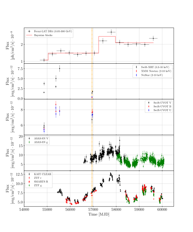
Figure 2: Multi-wavelength light curve of 5BZB J0630$-$2406 from $\gamma$-rays, X-rays to the optical band. The top panel shows the $\gamma$-ray light curve with one-yr binning, available from the 4FGL-DR4 catalog. The second panel displays measurements from Swift-XRT, XMM Newton and Nustar used for the modeling. The third panel shows values taken by Swift-UVOT in the three optical filters V, B, and U. The fourth panel shows the V-band and g-band data collected by ASAS-SN and the bottom panel shows the KAIT $Clear$ band measurement, the SMARTS R-band and the ZTF r-band and g-band. The X-ray and optical light curves are corrected for galactic extinction. The orange line highlights the time of quasi-simultaneous data used in the SED analysis. GROND data also used for modeling but not included in this panel are discussed in section 3.2.

3.4 X-ray observations

3.4.1 The Neil Gehrels Swift observatory

Overall, Swift-XRT (Gehrels et al. 2004) observed 5BZB J0630$-$2406 eight times, including visits during the period of the IceCube observations. To analyze the Swift-XRT data, the standard analysis tools provided by the HEASOFT V.6.31.1 software package were used.

The XRT observations were all in photon counting (PC) mode, and since the count rates were always below $0.5$ counts $\mathrm{s^{-1}}$, no pile-up correction was necessary. To extract the source events, a circular region with a radius of $45$” was chosen within the $0.3–10~{}\rm{keV}$ energy range. The background events were extracted from the annular region around the source position. Given the low photon statistics, we performed the spectral analysis with the Cash statistics method by rebinning the spectrum to ensure a minimum of one count per bin.

3.4.2 XMM-Newton and NuSTAR data reduction

5BZB J0630$-$2406  was targeted quasi-simultaneously by XMM-Newton (obsID: 0740820401; exposure: $9~{}\rm{ks}$) and NuSTAR (obsID: 60001140002; exposure: $66~{}\rm{ks}$) on October $17$–$18$, $2014$. We retrieved the XMM-Newton  pn source and background spectra and associated matrices from the 4XMM catalog (Webb et al. 2020). The source spectrum has been binned with $1$ count per bin, to avoid having empty bins that can affect the spectral fit. To generate the NuSTAR spectra, we followed the standard data reduction procedure. Specifically, the data have been processed using the NuSTAR Data Analysis Software (NUSTARDAS) version 2.1.1. The raw event files are calibrated by the nupipeline script, using the response file from the Calibration Database (CALDB) version 20210202. The source and background spectra are extracted from a $45^{\prime\prime}$ ($\approx 50\%$ of the encircled energy fraction at $10~{}\rm{keV}$) circular region, centered at the optical position of the source and in a nearby ($\sim$3^′ separation) region which was visually inspected to avoid any possible contamination, respectively. Using nuproducts scripts, we then generated source and background spectra files, along with the corresponding ARF and RMF files. Finally, the NuSTAR spectra are grouped with $1$ count per bin, using grppha. This procedure has been performed on both the NuSTAR focal plane modules, FPMA and FPMB.

3.5 XMM-Newton  and NuSTAR  spectral fitting results

We fitted the XMM-Newton  and NuSTAR spectra of our target using the XSPEC (Arnaud 1996) software, version 12.12.1. We fixed the metal abundance to Solar metallicity using the abundances from Wilms et al. (2000), while the photoelectric cross-sections for all absorption components are those derived by Verner et al. (1996). The Galactic absorption column density is fixed to $\rm{N}_{\rm H,gal}=7.5\times 10^{20}~{}\rm{cm}^{-2}$ (Kalberla et al. 2005). To maximize the spectral statistic, we analyze the data with the Cash statistic (Cash 1979), which uses a Poisson likelihood function and is hence most suitable for low numbers of counts per bin. As mentioned in the previous section, we bin the spectra with $1$ count per bin. The XMM-Newton  pn spectrum is fitted in the $0.3$–$10~{}\rm{keV}$ band, while the two NuSTAR  FPMA and FPMB spectra are fit in the $3$–$70~{}\rm{keV}$ band.

Following the standard procedure for fitting X-ray spectra of blazars, we first fit our data with a simple power-law model. We also add a cross-normalization constant to take into account the fact that the NuSTAR  observation is significantly longer than the XMM-Newton  one, and to model systematic cross-instrument offsets in flux. Finally, we include a column density at the redshift of the source, $N_{\rm H,z,ISM}$, assuming a redshift of $1.239$, to account for a possible contribution of the interstellar medium (ISM) to the absorption of X-ray photons. We measure a best-fit X-ray photon index $\Gamma_{\rm X}=3.03\pm 0.12$, with an ISM column density $N_{\rm H,z,ISM}=3.0_{-1.0}^{+1.1}\times 10^{21}~{}\rm{cm}^{-2}$, and a XMM-Newton–NuSTAR cross-normalization $\rm{C}_{\rm XMM-NuS}=1.90_{-0.34}^{+0.41}$. The best-fit statistic for this fit is $\rm{Cstat/d.o.f.}=1377.8/1408$.

We then fit the data with a log-parabola model, which has been shown to accurately describe the X-ray spectral shape of blazars (see, e.g., Bhatta et al. 2018). In particular, Middei et al. (2022) analyzed the NuSTAR  spectra of $126$ blazars and found that in some cases a log-parabola model provides a more statistically accurate description of a blazar X-ray spectrum. The log-parabola model is described by the following equation,

$$\dfrac{\rm{d}N}{\rm{d}E}=K\left(\frac{E}{E_{0}}\right)^{-\left({\alpha-\beta\log\left(E/E_{0}\right)}\right)},$$ (1)

where $E_{0}$ is the reference energy, which we fix as $5~{}\rm{keV}$ (in the observer frame) following the results of previous works (e.g., Massaro et al. 2004; Baloković et al. 2016; Middei et al. 2022), while $\alpha$ and $\beta$ are the photon index and the curvature parameter, respectively (e.g., Massaro et al. 2004), and $K$ is the model normalization.

The log-parabola component best-fit parameters are $\alpha=2.71_{-0.17}^{+0.19}$, $\beta=-0.42_{-0.20}^{+0.21}$, and $N_{\rm H,z,ISM}=5.5_{-1.7}^{+1.7}\times 10^{21}\rm{cm}^{-2}$, while the XMM-Newton–NuSTAR cross-normalization is $\rm{C}_{\rm XMM-NuS}=1.66_{-0.32}^{+0.39}$. The best-fit statistic for this fit is $\chi^{2}/\rm{d.o.f.}=1367.4/1407$. The difference in $\rm{Cstat}$ between this model and the simple power-law one is $\Delta\rm{Cstat}=1377.8-1367.4=10.4$. Since the log-parabola model has $1$ degree of freedom less than the simple power-law one, the log-parabola model is statistically preferred at the $\sim 99.9$ % confidence level (i.e., with a $\gtrsim 3.2\,\sigma$ significance).

Finally, we performed a fit with a broken power-law model, which is also commonly used to describe the X-ray spectra of blazars. The parameterization of the broken power-law is,

$$\frac{\rm{d}N}{\rm{d}E}=\begin{cases}KE^{-\Gamma_{1}}&\text{if }E\leq E_{\rm b}\,,\\ KE_{\rm b}^{\Gamma_{2}-\Gamma_{1}}(E/1\,{\rm keV})^{-\Gamma_{2}})&\text{otherwise.}\end{cases}$$ (2)

Here, $\Gamma_{1}$ and $\Gamma_{2}$ are the low and high-energy photon indexes, $K$ is the normalization parameter, and $E_{\rm b}$ is the (rest-frame) energy of the break. The best-fit parameters are $\Gamma_{1}=3.19_{-0.16}^{+0.17}$, $\Gamma_{2}=2.57_{-0.26}^{+0.24}$, $E_{\rm b}=6.3_{-2.2}^{+3.1}~{}\rm{keV}$ and $N_{\rm H,z,ISM}=4.2_{-1.3}^{+1.3}\times 10^{21}~{}\rm{cm}^{-2}$. The XMM-Newton–NuSTAR cross-normalization is $\rm{C}_{\rm XMM-NuS}=1.61_{-0.37}^{+0.55}$ The best-fit statistic for this fit is $\rm{Cstat/d.o.f.}=1365.5/1406$. The difference in $\rm{Cstat}$ between this model and the simple power-law one is $\Delta\rm{Cstat}=1377.8-1365.5=12.3$. Since the broken power-law model has $2$ fewer degree of freedom than the simple power-law one, the broken power-law model is statistically preferred at the $>99.8$ % confidence level (i.e., at a $\gtrsim 3.1~{}\sigma$ significance).

In summary, a two-component model is statistically favored with respect to a simple power-law one, while from a statistical point of view the log-parabola model and the broken power-law one are fully consistent. Differently from a previous study (Ackermann et al. 2016), our more sensitive analysis supports the presence of a break in the X-ray spectrum. We report in Fig. 3 the source light curves from both the NuSTAR  cameras and, as it can be seen, no clear variability trend is observed within the NuSTAR  observation. More in detail, we fit the two light curves with a constant and obtain best-fit count rates $r_{\rm FPMA}=0.45~{}\rm{cts}\cdot\rm{s}^{-1}$ and $r_{\rm FPMB}=0.44~{}\rm{cts}\cdot\rm{s}^{-1}$, with reduced chi square ($\chi^{2}/\rm{d.o.f.})_{\rm FPMA}=9.49/20$ and ($\chi^{2}/\rm{d.o.f.})_{\rm FPMB}=0.86/19$. We also note that the XMM-Newton–NuSTAR  cross-normalization values we measured in the log-parabola and broken power-law fits, while slightly higher than expected in quasi-simultaneous observations, have been observed in other XMM-Newton–NuSTAR  quasi-simultaneous observations (e.g., Marchesi et al. 2019) and may be explained by a simple cross-instrument calibration offset.

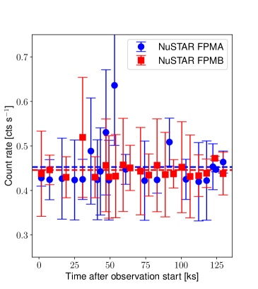
Figure 3: 5BZB J0630$-$2406 NuSTAR FPMA (blue circles) and FPMB (red squares) light curves. Both datasets are fit with a constant, shown with a blue (red) dashed line. No trend is observed in the light curves, suggesting no significant intra-observation variability in the NuSTAR data.

3.6 Fermi-Large Area Telescope observations

The study utilized gamma-ray data taken from Ackermann et al. (2016), and obtained from Fermi-LAT observations spanning the period between August $4$, $2008$, and January $31$, $2015$ within the energy range of $100$ MeV to $500$ GeV. This time period is contemporaneous to the simultaneous X-ray data introduced in the previous section.

4 Temporal Variability

The long-term optical light curves presented in Fig. 2 highlight a similar flux variability pattern over the monitored bands. According to the 4FGL-DR4 catalog (Ballet et al. 2023), the source is variable at $\gamma$-rays on $\gtrsim$ year-timescales. To characterize statistically-significant variations in the $\gamma$-ray light curve, we adopt the Bayesian algorithm available in Astropy (Astropy Collaboration et al. 2013). To determine the optimal value of the prior for the number of blocks, we use the empirical relation evaluated in Scargle et al. (2013) for the probability to falsely report a detection of a change point, setting it to $0.05$. Applying this approach to the yearly binned light curve, the first $\sim 7$-yr of LAT observations, up to $\sim$ MJD $57250$, are overall consistent with a steady state, indicating that if variability is present at these frequencies it may be below the sensitivity of the LAT data. During the more recent LAT observations, since $\sim$ MJD $57250$, the source is undergoing a long-term enhanced state.

Optical evidence of year-long modulations of the flux, on timescales of $\sim 3/4~{}\rm{yr}$. This is consistent with the behavior traced by the $>15$-yr $\gamma$-ray light curve, including a major flux enhancement observed around MJD $57800$. The sparse X-ray/UV data mimic the overall variability pattern at other frequencies. The high-cadence KAIT monitoring, with sampling as short as a $\sim 3~{}\rm{days}$ cadence, evidences statistically significant ($\gtrsim 6\sigma$) changes between consecutive observations (Ackermann et al. 2016). This suggests that at least some of the jet’s emission arises in compact $R\lesssim 10^{16}~{}\rm{cm}$ regions, in the observer’s frame.

5 Numerical SED modeling set up

5.1 Building the quasi-simultaneous broadband SED

In this work, we are mostly interested in the modeling of the MWL SED during the time span of the IceCube observations, i.e. $2008$-$2015$. Within this time range, MWL contemporaneous observations of 5BZB J0630$-$2406 were collected with the gamma-ray burst Optical/Near-Infrared Detector (GROND) instrument at the $2.2~{}\rm{m}$ MPG telescope at the ESO La Silla Observatory (Greiner et al. 2008), the Swift Niel Gehrels Observatory, XMM-Newton and NuSTAR (Harrison et al. 2013) satellites. They were performed around October $17$, $2014$ , i.e. $\sim~{}\rm{MJD}~{}56948$, close to the time period of the $7~{}\rm{yr}$ neutrino observations. These simultaneous ($\lesssim~{}1~{}\rm{day}$) multiwavelength data constrain the X-ray part of the synchrotron component. To constrain the second hump of the SED, we employ contemporaneous observations carried out by the $Fermi$-LAT in the MeV-GeV range. As discussed in Sec. 4, the source of interest is characterized by long-term variability in the $Fermi$-LAT band, and no significant variations in the flux are observed during the first $7$-yr of monitoring. Therefore, for the SED modeling we employ the LAT spectrum integrated over the first $7$ years of observations (from August $04$, $2008$ to August $15$, $2015$, i.e. MJD $54682-57250$) available from the literature (Ackermann et al. 2016). We exclude the UVOT data above $\nu\geq 10^{15}~{}\rm{Hz}$ as they are affected by the $\rm{Ly}\alpha$ forest absorption. Fig. 5 and Fig. 6 show the contemporaneous broadband SED built with these data (black points). Further archival radio, optical, and near-IR observations are displayed for comparison (gray points), and not included in the SED modeling. The red downward triangle represents a limit on accretion disk luminosity from Ghisellini et al. (2012).

5.2 One zone model

We explore different scenarios to describe the MWL emission of 5BZB J0630$-$2406 using the time-dependent code AM³ (Gao et al. 2017). This code is able to solve the system of coupled differential equations that describe the transport of particles through the relativistic jet. Relativistic electrons and protons are assumed to be accelerated initially and injected into a single zone where they can radiate their energy and interact with external photon fields. For more details on the implementation of the synchrotron, inverse Compton scattering, photo-photon pair annihilation, hadronic processes (i.e., Bethe-Heitler pair production and photo-pion production), we refer the reader to Gao et al. (2017). We also note that the synchrotron self-absorption opacity of the blob is treated only for the electrons (we expect a negligible contribution from the proton population in the radio band).

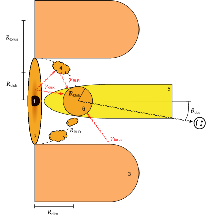
Figure 4: Schematic view of the model. 1: Supermassive black hole, 2: Accretion disk defined by a luminosity $L_{\rm disk}$ and a temperature $T_{\rm disk}$, 3: Dust torus defined by a luminosity $L_{\rm torus}$ and a temperature $T_{\rm torus}$, 4: Broad line region (BLR) that scattered direct emission, 5: Relativistic jet (not modeled here) and 6: Moving emission region (“blob”) situated at a distance $R_{\rm diss}$ from the black hole. Direct (indirect) external photon fields are represented by continuous (dashed) arrows. Scheme not to scale.

As represented in the Fig. 4, the emission region is modeled as a sphere of radius $R^{\prime}_{\rm b}$ that moves at relativistic speed with a Lorentz factor of $\Gamma_{\rm b}$. From Earth, the blob is observed with an observation angle $\theta_{\rm obs}=1/\Gamma_{\rm b}$, with quantities Doppler-shifted according to the Doppler factor $\delta_{\rm D}=\Gamma_{\rm b}$. A magnetic field with a strength of $B^{\prime}$ is assumed to be present in the blob and isotropic, i.e. with no preferential direction. The blob is located at a distance of $R_{\rm diss}$ from the supermassive black hole, also known as the dissipation radius, considered static here. Since the energy density of external photon fields varies with $R_{\rm diss}$, this parameter is a crucial aspect of our model.

In our model, relativistic electrons and/or protons are injected into the blob. For the electrons, we use a broken power-law distribution given by,

$$\dfrac{\rm{d}N_{\rm e}}{\rm{d}\gamma^{\prime}_{\rm e}}\propto\begin{cases}{\gamma^{\prime}_{\rm e}}^{-p_{\rm e,1}}&\text{for }\gamma^{\prime}_{\rm e,min}<\gamma^{\prime}_{\rm e}\leq\gamma_{\rm e,brk}\,,\\ {\gamma^{\prime}_{\rm e}}^{-p_{\rm e,2}}\cdot{\gamma^{\prime}_{\rm e,brk}}^{p_{\rm e,2}-p_{\rm e,1}}&\text{for }\gamma^{\prime}_{\rm e,brk}<\gamma^{\prime}_{\rm e}<\gamma^{\prime}_{\rm e,max}\,,\end{cases}$$ (3)

where $\gamma^{\prime}_{\rm e,min}$ and $\gamma^{\prime}_{\rm e,max}$ are the cut-off values, and $\gamma^{\prime}_{\rm e,brk}$ is the break energy. The choice of this distribution is supported by a pre-fit analysis on the observed SED that it used for initial guesses only (as it can be seen in Ghisellini et al. (2012)). For protons, we assume a simple power-law distribution,

$$\dfrac{\rm{d}N_{\rm p}}{\rm{d}\gamma^{\prime}_{\rm p}}\propto{\gamma^{\prime}_{\rm p}}^{-p_{\rm p}}~{}~{}~{}\text{for }\gamma^{\prime}_{\rm p,min}<\gamma^{\prime}_{\rm p}<\gamma^{\prime}_{\rm p,max}\,.$$ (4)

The parameters $N_{\rm e}$ and $N_{\rm p}$ are the normalization factors. We ensure that the constraints on $\gamma^{\prime}_{\rm e,brk}$ and $\gamma^{\prime}_{\rm e/p,max}$ are compatible by respectively equating the synchrotron cooling timescale $\tau_{\rm syn}$ with the adiabatic timescale $\tau_{\rm ad}=2R^{\prime}_{\rm b}/c$ and the acceleration timescale, $\tau_{\rm acc}$ with the shortest cooling timescale. For $\gamma^{\prime}_{\rm e/p,max}$, we also check that the Hillas criterion is satisfied.

Given the expected large redshift, we incorporate the effect of absorption by the extragalactic background light (EBL) in our model. To achieve this, we use the Python library ebltable, which is based on the model presented by Domínguez et al. (2011).

The presence of a luminous accretion disk and radiation fields has been suggested by previous literature studies (Ghisellini et al. 2012; Padovani et al. 2012). External radiation field radiation can either interact directly with the source in the jet or be re-processed by a broad line region (BLR). A dust torus is also present in this model, as its presence has been considered in numerous previous studies (Finke 2016; Murase et al. 2014; Oikonomou et al. 2021). An upper limit on the disk luminosity has been derived in Ghisellini et al. (2012),

$$L_{\rm disk}\leq 5.5\times 10^{45}~{}\rm{erg}\cdot\rm{s}^{-1}\,.$$ (5)

It was obtained assuming an empirical relation between the BLR and gamma-ray luminosities ($L_{\rm BLR}\sim 4\times L_{\rm\gamma}^{0.93}$).

Therefore, the model presented accounts for both external radiation fields originated either from the accretion disk and the dust torus, modeling them in the observer frame as a single temperature black body emission (Dermer & Menon 2009) for simplicity, as visible in Rodrigues et al. (2019). This choice is also motivated by the lack of optical lines, as it implies a higher uncertainty on the black hole mass and the disk type.

Following Ghisellini et al. (2017), we assume in this study that the luminosity and the size of the dust torus can be derived from the disk luminosity and the dust torus temperature,

$$L_{\rm torus} =L_{\rm disk}/2\,,$$ (6)

$$R_{\rm torus} =3.5\times 10^{18}~{}\left(\dfrac{L_{\rm disk}}{10^{45}~{}\rm{erg.s}^{-1}}\right)^{1/2}\cdot\left(\dfrac{T_{\rm torus}}{10^{3}~{}\rm{K}}\right)^{-2.6}\,.$$ (7)

where $L_{\rm disk}$, $T_{\rm disk}$, and $T_{\rm torus}$ are free parameters in the model. Our model assumes that the emission from the accretion disk is generated by a single-temperature black-body that interacts with the source jet through a Doppler de-boosting effect, which is proportional to $\Gamma_{\rm b}^{2}$. In fact, we consider a scenario in which a single-temperature accretion disk emits an isotropic radiation “behind” the blob, as the jet is pointing at the observer. The emission of the dust torus is boosted in the blob frame and also consider isotropic. Additionally, the emission can be scattered by the BLR, which we assume is modeled as a thin shell located at a distance $R_{\rm BLR}$ from the central engine and radiating the luminosity $L_{\rm BLR}$. Both $L_{\rm BLR}$ and $R_{\rm BLR}$ are derived following Ghisellini & Tavecchio (2008),

$$L_{\rm BLR} =10^{-1}\cdot L_{\rm disk}\,,$$ (8)

$$R_{\rm BLR} =10^{17}~{}\rm{cm}\cdot\left(\dfrac{L_{\rm disk}}{10^{45}~{}\rm{erg.s}^{-1}}\right)^{1/2}\,.$$ (9)

We assume that the BLR reprocesses $10\%$ of the disk emission isotropically in the rest frame of the black hole (Sbarrato et al. 2012). In fact, most of the reprocessed flux is emitted in emission lines (e.g. Lyman $\alpha$) and not as a thermal continuum (which accounts for $1\%$ (Blandford & Levinson 1995; Murase et al. 2014)). In fact, we consider that most of them will lie on the disk emission range (Lyman $\alpha$ is situated at $\sim 10^{15}~{}\rm{Hz}$) and are outshined by the non-thermal continuum from the jet (Rodrigues et al. 2021).
In the blob frame, this radiation field is enhanced by a factor $\delta^{2}$. This Doppler factor depends on $\Gamma_{\rm b}$ but also on the dissipation radius $R_{\rm diss}$, so that the energy density perceived by the blob will be lower outside the BLR radius, according to scaling factors calculated in Ghisellini & Tavecchio (2009).

To explore the parameter space, we develop a parameter search algorithm which is parallelized, with initial and mutation guesses stored on the first and successive central processing units (CPU), respectively. Gaussian noises are applied to each parameter as mutations. We use the least_squares function from the scipy.optimize library to optimize the parameters. For each parameter set and CPU, the algorithm calls the AM³ code, which returns the simulated SED. The optimization is based on minimizing the residuals. Finally, we select the parameter sets associated with the best $\chi^{2}/{\rm d.o.f.}$ value. Here, the $\rm{d.o.f.}$ term refers to the number of degrees of freedom. If the $\chi^{2}/{\rm d.o.f.}$ value is not acceptable, we use this latest set of parameters found as input for the next generation, with the other solutions being mutations of this one. The process stops when the $\chi^{2}/{\rm d.o.f.}$ value is sufficiently low, i.e., $\chi^{2}/{\rm d.o.f.}\leq 2$. More details on the parameter space research, and on the evaluation of initial guesses, are show in Appendix B.

6 SED modeling Results

6.1 Purely leptonic solution

In our initial attempt to model the SED of 5BZB J0630$-$2406, we considered only a population of relativistic electrons. The simulated SED is shown in Fig. 5, and the fitted parameters can be found in Table 1 labeled L. In this figure, the labels SY and IC stand respectively for synchrotron and inverse Compton, from either the leptonic population ($e^{\pm}$) or from $\gamma-\gamma$ pair productions. In this scenario, the data points until the X-ray are explained by synchrotron emission only. The GeV gamma-ray data are partly explained by synchrotron self-Compton (SSC). The best solution found in that scenario is close to equipartition with $u^{\prime}_{\rm e}/u^{\prime}_{\rm b}\sim 3.9$, where $u^{\prime}_{\rm e}$ is the electron energy density and $u^{\prime}_{\rm b}$ the magnetic energy density. It should be noted that we did not take into account the presence of cold protons in this model. Here, we derived a relatively high value for $\gamma_{\rm e,min}$, this can be due to the prior acceleration (injection) of a truncated power-law from a region closer to the black hole. The cooling process might also be inefficient for lower energies, leading to the development of the low energy tail outside the zone model here (Katarzyński et al. 2006), explaining the radio counterpart. In fact, the extended jet is expected to contribute to the integrated radio flux where those low energy electrons will cool down (Plavin et al. 2022). Such a model is beyond the scope of this paper. Specific interactions between the electron and proton populations can also explain high $\gamma_{\rm e,min}$ values (Zech & Lemoine 2021).

To account for the limit proposed by Ghisellini et al. (2012), we included the black body emission of the accretion disk. The final disk luminosity obtained is $L_{\rm disk}=4.8\times 10^{45}~{}\rm{erg}\cdot\rm{s}^{-1}$, which explains the peaky feature observed at the highest $\gamma$-ray energies with external Compton interactions. In this model, the blob is located at a dissipation radius of $R_{\rm diss}/R_{\rm BLR}=1.7$, indicating that the influence of the BLR radiation field is still significant. The dust torus black body is also present but subdominant.

From the accretion disk parameters obtained, we can derive a black hole mass of $\sim 10^{10}M_{\odot}$ and an associated Eddington luminosity of $\sim 3\times 10^{48}~{}\rm{erg}\cdot\rm{s}^{-1}$. As suggested in Sbarrato et al. (2012), we use the accretion regime $\eta=L_{\rm BLR}/L_{\rm Edd}$ as physical criteria to distinguish BL Lacertae (BL Lacs) from FSRQs. We find an accretion regime of $\eta\sim 2\times 10^{-4}$, close to the boundary that separates FSRQs from BL Lacs ($\eta=5\times 10^{-4}$, Sbarrato et al. 2012). Finally, the shortest timescale variability $\tau_{\rm var}$ derived from this model is $3.7~{}\rm{days}$ in the observer’s frame, close to the derived value from optical variability.

Given the X-ray spectrum, we further tested the possibility to reproduce the break in the X-ray band with the purely leptonic model, but we were not able to find an acceptable solution ($\chi^{2}_{\rm d.o.f.}\leq 2$, by lowering $\gamma_{\rm e,min}$ for example). This suggests that, if the break is present, it may be interpreted as the presence of additional processes. As we discuss in the following sections, a hadronic component is capable to successfully account for the broken spectral shape observed in the X-ray band as well as the putative neutrino emission.

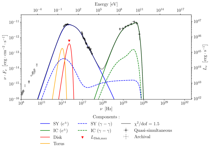
Figure 5: Spectral energy distribution from the purely leptonic model of 5BZB J0630$-$2406  in the observer frame. The dotted-dashed curves represent synchrotron and inverse Compton from pair production due to gamma-gamma absorption. The black solid squares represent the contemporaneous MWL data used for the modeling. Archival data are shown by gray solid dots. The red downward triangle represents the accretion disk limit from (Ghisellini et al. 2012).

6.2 Lepto-hadronic solution

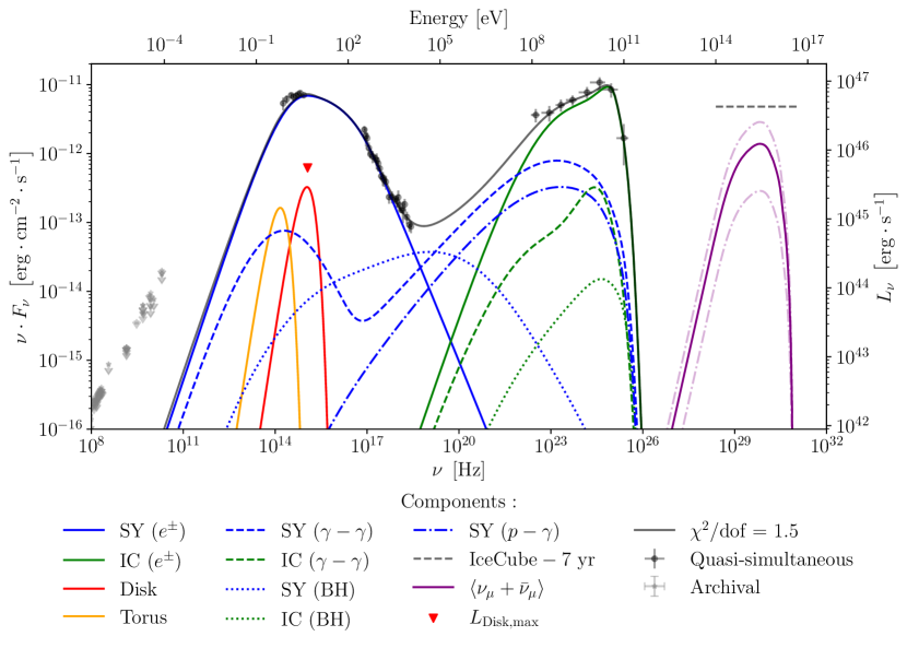
Figure 6: Same as Fig. 5 with the lepto-hadronic solution of 5BZB J0630$-$2406 in the observer frame. Dashed curves represent hadronic processes (BH (Bethe-Heitler) and photo-pion productions). The dotted-dashed blue curves represent the obtained muon neutrino flux with associated uncertainties from Poisson statistic assuming a $3\sigma$ levels.

We use the parameters found in the purely leptonic solution as starting point for the parameter space research of the lepto-hadronic scenario. The final parameters are displayed in the Tab. 1, labeled as LH, and the SED is displayed on the Fig. 6. Here BH stands from Bethe-Heitler reaction, while $p-\gamma$ stands for photo-pion production. Protons are injected with a simple power-law index of $2.0$ and the hadronic processes remain globally sub-dominant, except in the X-ray and MeV bands. Within the lepto-hadronic solution, we find values that are in agreement with those found for the purely leptonic model with an accretion regime of $\eta\sim 2\times 10^{-4}$, and an Eddington luminosity of $\sim 3\times 10^{48}~{}\rm{erg}\cdot\rm{s}^{-1}$. Similarly, the shortest timescale variability derived here, $\tau_{\rm var}\sim 3.3~{}\rm{days}$, is consistent with the value derived from optical variability. The cascade component accounts for the X-ray flux, particularly at the highest energy.

The higher energy MWL peak is mainly explained by SSC and EC interactions with the BLR, consistently with the pure leptonic solution. Similarly, we find a dissipation radius close to $1.6~{}R_{\rm BLR}$. The cascade component accounts for the hard X-ray data, leading to a steeper index for the electron broken power-law. Indeed, significant contributions from $\gamma-\gamma$ pair production in the GeV energy band can also be observed, which are more pronounced than the ones observed in the leptonic model due to the additional photon fields from mesons disintegration. Although the model finds $u^{\prime}_{\rm p}/u^{\prime}_{\rm b}\sim 10^{3}$ (where $u^{\prime}_{\rm p}$ is the proton energy density), far from the equipartition, the proton luminosity remains below the Eddington limit.

The model presented here may be considered a viable solution for the efficient neutrino production case found by our modeling. As the X-ray data provide upper-limits for the cascade component, a broad range of solutions can be obtained with less energetic protons and, hence, lower predicted neutrino fluxes.

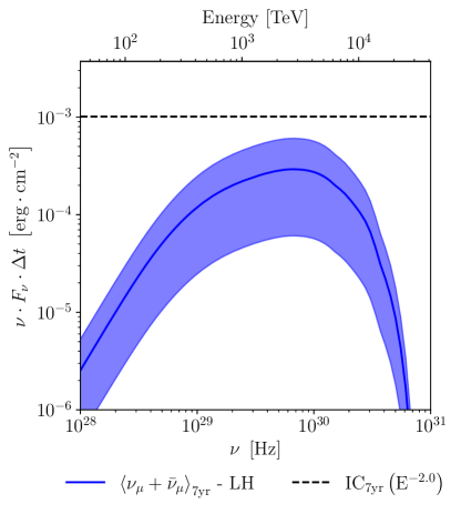
Figure 7: Neutrino flux scaled according to the livetime showed in Aartsen et al. (2017c) derived for both mixed lepto-hadronic modeling of 5BZB J0630$-$2406. The uncertainties are computed assuming Poisson statistics and $3\sigma$ levels. The dashed gray line represents the $7$-years IceCube sensitivity, assuming $E^{-2}$ and $\delta=-24\degree.06$.

Table 1: Parameters used for the leptonic and the mixed lepto-hadronic models.

	L	LH
$\delta_{\rm D}$	$22.7$	$22.5$
$R^{\prime}_{\rm b}~{}\left[\rm{cm}\right]$	$1.1\times 10^{17}$	$9.8\times 10^{16}$
$\tau_{\rm var}~{}\left[\rm{days}\right]$	$3.7$	$3.3$
$B^{\prime}~{}\left[\rm{G}\right]$	$6.4\times 10^{-2}$	$8.3\times 10^{-2}$
$u^{\prime}_{\rm b}~{}\left[\rm{erg}\cdot\rm{cm}^{-3}\right]$	$2.7\times 10^{-4}$	$3.1\times 10^{-4}$
$\gamma^{\prime}_{\rm e,min}$	$10^{4}$	$10^{4}$
$\gamma^{\prime}_{\rm e,brk}$	$1.1\times 10^{5}$	$1.3\times 10^{5}$
$\gamma^{\prime}_{\rm e,max}$	$9.6\times 10^{7}$	$1.0\times 10^{8}$
$p_{\rm e,1}$	$2.71$	$2.73$
$p_{\rm e,2}$	$3.84$	$4.26$
$u^{\prime}_{\rm e}~{}\left[\rm{erg}\cdot\rm{cm}^{-3}\right]$	$6.4\times 10^{-4}$	$6.3\times 10^{-4}$
$u^{\prime}_{\rm e}/u^{\prime}_{\rm b}$	$3.9$	$2.3$
$L^{\prime}_{\rm e}~{}\left[\rm{erg}\cdot\rm{s}^{-1}\right]$	$1.2\times 10^{42}$	$1.0\times 10^{42}$
$\gamma^{\prime}_{\rm p,min}$	$-$	$90$
$\gamma^{\prime}_{\rm p,max}$	$-$	$1.0\times 10^{7}$
$p_{\rm p}$	$-$	$2.0$
$u^{\prime}_{\rm p}~{}\left[\rm{erg}\cdot\rm{cm}^{-3}\right]$	$-$	$1.5$
$u^{\prime}_{\rm p}/u^{\prime}_{\rm b}$	$-$	$5.3\times 10^{3}$
$L^{\prime}_{\rm p}~{}\left[\rm{erg}\cdot\rm{s}^{-1}\right]$	$-$	$1.0\times 10^{45}$
$L_{\rm disk}~{}\left[\rm{erg}\cdot\rm{s}^{-1}\right]$	$4.8\times 10^{45}$	$3.9\times 10^{45}$
$T_{\rm disk}~{}\left[\rm{K}\right]$	$1.4\times 10^{4}$	$1.3\times 10^{4}$
$T_{\rm torus}~{}\left[\rm{K}\right]$	$1.3\times 10^{3}$	$1.3\times 10^{3}$
$R_{\rm diss}/R_{\rm BLR}$	$1.7$	$1.6$
$N_{\rm events}$ per year	$-$	$0.68^{+2.32}_{-0.68}$
$N_{\rm events}$ (total)	$-$	$4.82^{+5.18}_{-3.82}$
$\chi^{2}/{\rm{d.o.f.}}$	$1.5$	$1.5$

7 Discussion

Although still widely used, the historical classification of blazars based purely on observational characteristics, e.g. the optical spectrum and the location of the low-energy peak, has been put into question for a long time. Since the availability of large samples of blazars, thanks to $Fermi$-LAT observations, Ghisellini et al. (2011) has debated in favor of a more physical distinction for blazars based on the luminosity of the BLR measured in the Eddington units. Indeed, the BLR and Eddington luminosities are respectively related to the optical spectrum and the jet power (energy injected in the primary relativistic electrons). This can set a divide approximately where the disc transitions from a radiatively efficient to an inefficient regime.

Prior to being included in the sample of PeVatron blazars and proposed as a high-energy neutrino emitter, 5BZB J0630$-$2406 stood out in the literature due to its peculiarities. Historically, it has been classified as a BL Lac object due to the featureless optical spectrum and its high synchrotron peak, with $\nu_{\rm pk}^{\rm sy}\sim 10^{15}~{}\rm{Hz}$. 5BZB J0630$-$2406  was pinpointed as an exemplary blazar, it displays properties typical of “blue flat spectrum radio quasar” (Ghisellini et al. 2011; Padovani et al. 2012; Ghisellini et al. 2012, a.k.a. “high-power high-synchrotron-peak blazars”), i.e. high-emitting power sources that are intrinsically FSRQs where their broad emission lines are swamped by the jet synchrotron emission. For reference, this typology of blazars has also been called “masquerading BL Lacs” (Giommi et al. 2013; Padovani et al. 2019a). In contrast to “true” high-frequency-peaked BL Lacs which have intrinsically poor radiation fields, these objects host powerful jets and radiatively efficient accretion.

The study presented here allows us to provide conclusive evidence to the earlier speculations regarding the peculiar nature of 5BZB J0630$-$2406. The SED modeling reveals a bright accretion disk with $L_{\rm disk}\sim 4\times 10^{45}~{}\rm{erg}\cdot\rm{s}^{-1}$. The presence of external fields that are partly re-processed by the BLR naturally explains the peaky feature in the $\gamma$-ray band. Its accretion regime, i.e. the energy injected into these external fields, is of the order of $L_{\rm BLR}/L_{\rm Edd}\sim 2\times 10^{-4}$, close to the values physically suggested for FSRQs (Ghisellini et al. 2011). The relatively high accretion regime of 5BZB J0630$-$2406  is supported also by the ratio of the $\gamma$-ray luminosity $L_{\gamma}\left(0.1-100~{}\rm{GeV}\right)$ and the Eddington luminosity, $L_{\gamma}/L_{\rm Edd}\simeq 0.15$, highlighting that this source shares properties common to the FSRQ class (Sbarrato et al. 2012).

The location of the emitting region, outside but close to the BLR radius, makes the BLR radiation influence on the blob still important while at the same time it limits the absorption of $\gamma$-rays, leading to a bright $\gamma$-ray luminosity. We find that in 5BZB J0630$-$2406 the combination of an efficient particle acceleration ($E_{\rm p,max}\simeq 10^{19}~{}\rm{eV}$) and efficient external radiation fields fosters the production of neutrinos, similarly to TXS 0506$+$056 and PKS 1424$+$240, suggested as promising candidate neutrino emitters (Padovani et al. 2019a, 2022a, 2022b).

Here, we propose a scenario of mixed lepto-hadronic models, where protons are injected with various energies. It is important to note that these solutions are conservative in terms of the total power injected into the hadrons. Emission from secondary particles in these models are mostly sub-dominant, although they can account for the hard X-ray and in the MeV bands. In fact, the broken spectral shape in the X-ray data suggests the presence of underlying processes.

8 Neutrinos from 5BZB J0630$-$2406

To estimate the number of neutrinos predicted in the lepto-hadronic scenario, we compute the energy flux for different flavors of neutrinos in the observer frame, and we consider the actual number of $\mu$-neutrinos according to oscillations. To account for the detection efficiency, we use tabulated effective areas from the point-source analysis of the IceCube detector in its final configuration with $86$ strings (IC$86$, Aartsen et al. 2017c), at the declination of 5BZB J0630$-$2406 ($\delta=-24^{\circ}.06$). We utilize the published effective areas presented in Aartsen et al. (2017c), for each previous configurations: IC$40$, IC$59$, IC$79$ and IC$86$. To determine the expected number of events, we integrate the flux over the energy range observed by IceCube ($300$ TeV - $1$ EeV) using the given effective area and over a period of $\sim 7$ years, which is the full livetime of the observations used in Buson et al. (2022a). For reference, we also display the IceCube $7$-year flux sensitivity derived at $\delta=-24\degree.06$ and assuming a neutrino spectrum of $E^{-2}$ (Aartsen et al. 2017b).

The expected flux of $\mu$-neutrinos as observed on Earth is shown in Fig. 7 and is close to the IceCube sensitivity (Aartsen et al. 2017b, estimated for a $\propto E^{-2}$ spectrum). Our lepto-hadronic model predicts $N_{\rm events}=4.82^{+5.18}_{-3.82}$ over a livetime period of $7$ years, as shown on Fig. 8. Fig. 8 shows the temporal evolution of the number of events $N_{\rm events}$ assuming a constant flux over the livetime of the IceCube detector, accounting for the different strings configurations, with $3\sigma$ uncertainties. Assuming low counting statistics, e.g. Poisson statistics, we can evaluate the probability of $N_{\rm events}$ detection against a null hypothesis of no detection, under the form of a $p$-value. Considering the first $7$-year livetime Aartsen et al. (2017c), we find a $p$-value of $0.03$, indicating a small tension with the null hypothesis of no detection. It should be noted that, in the most conservative scenario, our model still predicts a minimum of $N_{\rm min}=4.82-3.82=1$ event, with a $p$-value higher than $0.05$. We find that 5BZB J0630$-$2406  contributes for $\leq 1\%$ to the IceCube diffuse muon neutrino flux (IceCube Collaboration et al. 2022). Similar values were obtained for TXS 0506$+$056 (Aartsen et al. 2016; IceCube Collaboration et al. 2018c).

Figure 8: Evolution of the number of observed events by the IceCube detector in time according to various string configurations, and assuming a constant flux. The uncertainties are evaluated assuming Poisson statistics ($3\sigma$ levels). The blue dashed line represents the integrated livetime used in Buson et al. (2022a).

We can derive the baryonic loading in the blob frame, which represents the ratio between the proton luminosity and the $\gamma$-ray luminosity, denoted by $\xi=L^{\prime}_{\rm p}/L^{\prime}_{\rm\gamma}$. Based on our lepto-hadronic model, we find a loading factor of $\xi\sim 10^{3}$. This value appears notably high when compared to the typical order of magnitude, which is around $100$ as derived in Murase et al. (2014). Nevertheless, the value obtained here is consistent with the range derived in Palladino et al. (2019), as the intermediate BL Lac - FSRQ objects show a higher $\xi$, but still respecting the IceCube stacking limit (Aartsen et al. 2015). Appendix A discusses our findings in the context of literature studies that tackled 5BZB J0630$-$2406 as an ultra-high-energy cosmic ray (UHECR) candidate.

9 Conclusions

5BZB J0630$-$2406 has been recently proposed as a high-energy neutrino emitter based on the observation of a statistically significant spatial correlation with high-energy IceCube data. To address the plausibility of this association from the theoretical perspective, in this work we analyze simultaneous and quasi-simultaneous multi-wavelength data of the blazar, and model the emission of the source using a one-zone model in the context of both a purely leptonic and mixed lepto-hadronic scenario.
We summarize the main findings in the following.

• Despite being formally classified as a high-synchroton-peaked BL Lac object, based on its featureless optical spectrum, the intrinsic nature of 5BZB J0630$-$2406 is that of a high-power FSRQ. It hosts a standard accretion disk and BLR; the optical emission lines elude direct observation, being the optical band swamped by the non-thermal continuum. The combination of efficient external radiation fields and enhanced particle acceleration efficiency offers ideal conditions for the production of neutrinos.

• The presence of a bright accretion disk is confirmed by a peaky feature in the $\gamma$-ray spectrum at the highest observable LAT energies. In FSRQ sources, a similar spectral shape may be observed and is naturally explained by external Compton reprocessing of the disk/BLR radiation by the jet.

• The SED can be adequately modeled via both purely leptonic and mixed lepto-hadronic scenarios, suggesting that the hadronic component is sub-dominant except in the X-ray and in the MeV bands. Our results predict that future missions in the MeV band, such as AMEGO-x and ASTROGAM (Caputo et al. 2022; De Angelis et al. 2021), hold the power to discriminate between these models.

• The analysis of the simultaneous XMM-Newton and NuSTAR  spectra during a comparatively low state, provides evidence ($\gtrsim 3\sigma$) of a break in the X-ray band. If the break was to be intrinsic to the object, a pure leptonic model faces challenges in reproducing it. On the other hand, the proposed lepto-hadronic model shows a turnover of the spectrum in the X-ray band, that marks the kick-in of the hadronic component contribution. Based on our theoretical modeling, the SED is overall leptonic-dominated. Therefore, observations in lower activity states, as the one studied here, may offer better chances to pinpoint the hadronic fingerprint.

• The relatively high accretion regime of 5BZB J0630-2406 is supported also by the ratio of the $\gamma$-ray luminosity $L_{\gamma}\left(0.1-100~{}\rm{GeV}\right)$ and the Eddington luminosity, $L_{\gamma}/L_{\rm Edd}\simeq 0.15$. As further reprove of the intrinsic FSRQ nature, the model reveals an efficient accretion regime of $2\times 10^{-4}$. Besides, a relatively large fraction of the $\gamma$-ray luminosity ($\sim 15\%$ of $L_{\rm Edd}$) is observed. Similarities can be found with the object TXS 0506+056 (Padovani et al. 2019b), where the localization of the $\gamma$ emission region is thought to be, as in our case, on the edge of the BLR avoiding a significant $\gamma-\gamma$ absorption and an efficient neutrino production.

• The neutrino emission predicted within the lepto-hadronic framework is at reach of the IceCube detector, close to the flux sensitivity. During the $7$-yr integration span of the data used in Buson et al. (2022a), we expect to observe $N_{\rm events}=4.82^{+5.18}_{-3.82}$ neutrinos. Assuming that the object maintains a constant neutrino rate over time, more high-energy neutrinos may be expected with increased instrument exposure. However, the uncertainties on the predicted numbers are large and long-term variability in the MWL light curve is clearly present at almost all observable frequencies.

• The contribution of 5BZB J0630$-$2406 to the astrophysical neutrino diffuse flux is expected to be of the order of $\sim 1\%$.

Based on the theoretical predictions presented here, the PeVatron blazar 5BZB J0630$-$2406 is capable of producing neutrinos in the IceCube energy range and can plausibly contribute to the anisotropy observed in the distribution of IceCube events of the hotspot IC J0630$-$2353 (see Fig. 1, Buson et al. 2022a). 5BZB J0630$-$2406 is a high-power, radiatively efficient blazar. Other objects in the PeVatron blazar sample display similar characteristics, i.e. TXS 0506$+$056, PKS 1424$+$240 and 5BZB J0035$+$1515 (Buson et al. 2022a, b). At the current status it remains unclear whether this peculiar, relatively rare characteristic describes the persistent behavior of their engine and/or is linked to different environment properties, or may be tracing temporary physical changes, such as changes in the state of the accretion mode, as suggested for “changing-look blazars” (Peña-Herazo et al. 2021), or changes in the location of the dissipation region (Ghisellini et al. 2013). Future investigation of the PeVatron blazar sample will enable us with a broader understanding of the neutrino/blazar physical relation.

The authors thank the anonymous reviewer for the valuable comments and constructive feedback. The authors thank Andreas Zech, Anita Reimer, Markus Böttcher and Jörn Wilms for the fruitful discussions, and Weikang Zehng for providing the calibrated KAIT data. GFDC thanks Xavier Rodrigues for the essential help with AM³. This work was supported by the European Research Council, ERC Starting grant MessMapp, S.B. Principal Investigator, under contract no. 949555. This research has made use of the NASA/IPAC Extragalactic Database, which is funded by the National Aeronautics and Space Administration and operated by the California Institute of Technology (the NASA/IPAC Extragalactic Database (NED) is funded by the National Aeronautics and Space Administration and operated by the California Institute of Technology). Part of this work is based on observations obtained with the Samuel Oschin Telescope $48$-inch and the $60$-inch Telescope at the Palomar Observatory as part of the Zwicky Transient Facility project. ZTF is supported by the National Science Foundation under Grant No. AST-2034437 and a collaboration including Caltech, IPAC, the Weizmann Institute for Science, the Oskar Klein Center at Stockholm University, the University of Maryland, Deutsches Elektronen-Synchrotron and Humboldt University, the TANGO Consortium of Taiwan, the University of Wisconsin at Milwaukee, Trinity College Dublin, Lawrence Livermore National Laboratories, and IN2P3, France. Operations are conducted by COO, IPAC, and UW. We acknowledge support by Institut Pascal at Université Paris-Saclay during the Paris-Saclay Astroparticle Symposium 2021 and 2022, with the support of the P2IO Laboratory of Excellence (program “Investissements d’avenir” ANR-11-IDEX-0003-01 Paris-Saclay and ANR-10-LABX-0038), the P2I axis of the Graduate School Physics of Université Paris-Saclay, as well as IJCLab, CEA, IPhT, IAS, OSUPS, the IN2P3 master projet UCMN, APPEC, and EuCAPT.

Appendix A An ultra-high-energy cosmic-ray event in the direction of 5BZB J0630$-$2406

An ultra-high-energy cosmic ray (UHECR) event has been observed in 2007 by the Pierre-Auger observatory, with an observed energy of $E_{\rm cr}=60~{}\rm{EeV}$ and celestial coordinates $\rm{RA},~{}DEC=105.9,-22.9$ ($l,~{}b=-125.2,-7.7$, Aab et al. 2015). The blazar 5BZB J0630$-$2406 is located at an angular distance of $\theta=7.6\degree$ from the UHECR event, and a previous study has considered it as a candidate counterpart (Resconi et al. 2017). Based on our theoretical modeling of 5BZB J0630$-$2406, the maximum energy reached by the protons in the co-moving frame is $E^{\prime}_{\rm p,max}\simeq 0.01~{}\rm{EeV}$. This translates to a maximum proton energy of $E_{\rm p,max}\simeq 0.2~{}\rm{EeV}$ in the observer frame, that is below the value of the ultra-high-energy observed. Cosmic rays propagate with Larmor radii $r_{\rm L}=1.1~{}\rm{Mpc}\;E_{EeV}/(Z\times B_{\rm nG})$, where $E$ is the cosmic ray energy, $Z$ the atomic number and $B$ the magnetic field. Using Hillas criterion and a minimal extragalactic magnetic field strength of $B=1~{}\rm{nG}$, for the source of interest one can derive the Larmor radius of $R_{\rm L,cr}\simeq 66~{}\rm{kpc}$, which represents the typical length scale of scattering and deflections. PeV-scale protons will scatter at the kpc scale, even for magnetic fields as weak as nG. In the vicinity of the source, the magnetic field may be much stronger, in which case the scattering/deflection length is even shorter. Consequently, at PeV-EeV energies, protons from cosmological distances are expected to be completely isotropized. It is therefore not possible to trace back the UHCRs to sources such as the one of interest here.

Appendix B Parameter space research

To explore the parameter space for a given scenario, we developed a comprehensive approach based on minimizing the residuals between the simulated and observed SEDs. This minimization method optimizes the goodness of fit by evaluating the reduced chi-squared ($\chi^{2}/{\rm d.o.f.}$) value. The flow chart of the optimization algorithm is illustrated in Fig. 9.
The first step involves a pre-fit of the observed SED (similar to Ghisellini et al. (2012)). Assuming that the first bump-like feature arises from synchrotron emission by electrons, we can determine the values of $\gamma^{\prime}_{\rm e,min}$, $\gamma^{\prime}_{\rm e,break}$, and $\gamma^{\prime}_{\rm e,max}$. Linear regression on data points within a given energy band enables us to derive spectral indices in both branches of the broken power-law distribution ($\alpha_{\rm e,1}$ and, $\alpha_{\rm e,2}$ respectively). The result of the pre-fit analysis is shown in the Fig. 10.

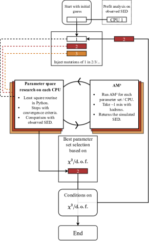
Figure 9: Flow chart of the parameter space research algorithm used in this study. A box labeled by a number represent a set of parameters for a given CPU.

Assuming a broken power-law and synchrotron cooling, we find respectively $p_{\rm e,1}=2.65$ and $p_{\rm e,2}=3.69$. Furthermore, we can derive the energies in the jet frame as follows,

$$\gamma^{\prime}_{\rm e,min} =A_{\rm e,min}\cdot B^{\prime-1/2}/\delta_{\rm D}\cdot\left(1+z\right)\,,$$ (B1)

$$\gamma^{\prime}_{\rm e,brk} =A_{\rm e,brk}\cdot B^{\prime-1/2}/\delta_{\rm D}\cdot\left(1+z\right)\,,$$ (B2)

$$\gamma^{\prime}_{\rm e,max} =A_{\rm e,max}\cdot B^{\prime-1/2}/\delta_{\rm D}\cdot\left(1+z\right)\,,$$ (B3)

where we have $A_{\rm e,min}=1.7\times 10^{2}$, $A_{\rm e,brk}=4.5\times 10^{4}$ and $A_{\rm e,max}=8\times 10^{5}$, the associated Lorentz factor obtained for values of Doppler factor $\delta_{\rm D}=25$, magnetic field strength $B^{\prime}=0.1~{}\rm{G}$ and redshift $z=1.239$. We also note that from the fit, we found $\nu_{\rm e,min}=1.1\times 10^{11}~{}\rm{Hz}$, $\nu_{\rm e,brk}=8\times 10^{15}~{}\rm{Hz}$ and $\nu_{\rm e,max}=2.72\times 10^{18}~{}\rm{Hz}$.

Concerning $\gamma^{\prime}_{\rm e,min}$, we assume here that the radio flux corresponds to the integrated synchrotron emission along the jet, in the synchrotron self-absorption regime (assuming a spectral index $\alpha=5/2$).
Finally, we used a log-parabola fit on both peaks to estimate the bolometric luminosity $L_{\rm bol}\sim 7.3\times 10^{47}~{}\rm{erg}\cdot\rm{s}^{-1}$. This implies that the injected energy in the electrons should not exceed $L_{\rm bol}/\Gamma_{\rm D}^{2}$. These derived quantities were used as the initial guess.

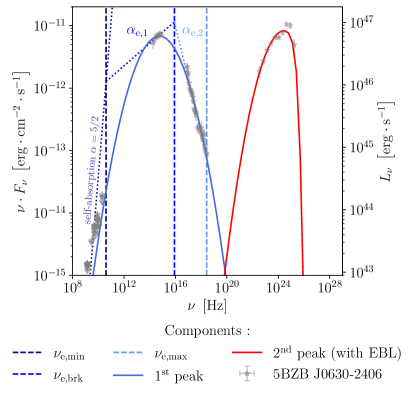
Figure 10: Pre-analyzed observed SED showing the first peak, assumed to be due to synchrotron emission from relativistic electrons, and the second peak. Assuming a Doppler factor $\delta_{\rm D}$, a magnetic field strength $B^{\prime}$ (and the source redshift $z$), one can derive characteristics of the electron distribution, including the minimum, break, maximum energies and both indexes are indicated in the legend.

References

- Aab et al. (2015) Aab, A., Abreu, P., Aglietta, M., et al. 2015, ApJ, 804, 15
- Aartsen et al. (2017a) Aartsen, M. G., Abraham, K., Ackermann, M., et al. 2017a, ApJ, 835, 45
- Aartsen et al. (2015) —. 2015, ApJ, 809, 98
- Aartsen et al. (2016) Aartsen, M. G., Abraham, K., Ackermann, M., et al. 2016, The Astrophysical Journal, 833, 3. https://dx.doi.org/10.3847/0004-637X/833/1/3
- Aartsen et al. (2017b) Aartsen, M. G., Abraham, K., Ackermann, M., et al. 2017b, ApJ, 835, 45
- Aartsen et al. (2017c) —. 2017c, ApJ, 835, 151
- Aartsen et al. (2020) Aartsen, M. G., Ackermann, M., Adams, J., et al. 2020, Phys. Rev. Lett., 124, 051103
- Abbasi et al. (2021) Abbasi, R., Ackermann, M., Adams, J., et al. 2021, arXiv e-prints, arXiv:2111.10169
- Abbasi et al. (2023) —. 2023, arXiv e-prints, arXiv:2304.01174
- Ackermann et al. (2016) Ackermann, M., Ajello, M., An, H., et al. 2016, ApJ, 820, 72
- Arnaud (1996) Arnaud, K. A. 1996, in Astronomical Society of the Pacific Conference Series, Vol. 101, Astronomical Data Analysis Software and Systems V, ed. G. H. Jacoby & J. Barnes, 17
- Astropy Collaboration et al. (2013) Astropy Collaboration, Robitaille, T. P., Tollerud, E. J., et al. 2013, A&A, 558, A33
- Azzollini et al. (2023) Azzollini, A., Buson, S., Coleiro, A., et al. 2023, in 38th International Cosmic Ray Conference (ICRC2023), Vol. 444 (Proceedings of Science)
- Ballet et al. (2023) Ballet, J., Bruel, P., Burnett, T. H., Lott, B., & The Fermi-LAT collaboration. 2023, arXiv e-prints, arXiv:2307.12546
- Baloković et al. (2016) Baloković, M., Paneque, D., Madejski, G., et al. 2016, ApJ, 819, 156
- Bellenghi et al. (2023) Bellenghi, C., Padovani, P., Resconi, E., & Giommi, P. 2023, arXiv e-prints, arXiv:2309.03115
- Bessell et al. (1998) Bessell, M. S., Castelli, F., & Plez, B. 1998, A&A, 333, 231
- Bhatta et al. (2018) Bhatta, G., Mohorian, M., & Bilinsky, I. 2018, A&A, 619, A93
- Blandford et al. (2017) Blandford, R., Yuan, Y., Hoshino, M., & Sironi, L. 2017, Space Science Reviews, 207, 291
- Blandford & Levinson (1995) Blandford, R. D., & Levinson, A. 1995, ApJ, 441, 79
- Bonning et al. (2012) Bonning, E., Urry, C. M., Bailyn, C., et al. 2012, ApJ, 756, 13
- Breeveld et al. (2011) Breeveld, A. A., Landsman, W., Holland, S. T., et al. 2011, in American Institute of Physics Conference Series, Vol. 1358, Gamma Ray Bursts 2010, ed. J. E. McEnery, J. L. Racusin, & N. Gehrels, 373–376
- Brightman et al. (2014) Brightman, M., Nandra, K., Salvato, M., et al. 2014, MNRAS, 443, 1999
- Buson et al. (2022a) Buson, S., Tramacere, A., Pfeiffer, L., et al. 2022a, ApJ, 933, L43
- Buson et al. (2022b) —. 2022b, ApJ, 934, L38
- Buson et al. (2023) Buson, S., Tramacere, A., Oswald, L., et al. 2023, arXiv e-prints, arXiv:2305.11263
- Caputo et al. (2022) Caputo, R., Ajello, M., Kierans, C. A., et al. 2022, Journal of Astronomical Telescopes, Instruments, and Systems, 8, 044003
- Cash (1979) Cash, W. 1979, ApJ, 228, 939
- Cerruti et al. (2018) Cerruti, M., Zech, A., Boisson, C., et al. 2018, Monthly Notices of the Royal Astronomical Society: Letters, 483, L12. https://doi.org/10.1093/mnrasl/sly210
- Cerruti et al. (2015) Cerruti, M., Zech, A., Boisson, C., & Inoue, S. 2015, MNRAS, 448, 910
- Cohen et al. (2014) Cohen, D. P., Romani, R. W., Filippenko, A. V., et al. 2014, The Astrophysical Journal, 797, 137. https://dx.doi.org/10.1088/0004-637X/797/2/137
- De Angelis et al. (2021) De Angelis, A., Tatischeff, V., Argan, A., et al. 2021, Experimental Astronomy, 51, 1225
- Dermer & Menon (2009) Dermer, C. D., & Menon, G. 2009, High Energy Radiation from Black Holes: Gamma Rays, Cosmic Rays, and Neutrinos
- Dermer et al. (2014) Dermer, C. D., Murase, K., & Inoue, Y. 2014, Journal of High Energy Astrophysics, 3, 29
- Domínguez et al. (2011) Domínguez, A., Primack, J. R., Rosario, D. J., et al. 2011, Monthly Notices of the Royal Astronomical Society, 410, 2556. https://doi.org/10.1111/j.1365-2966.2010.17631.x
- Fichet de Clairfontaine et al. (2022) Fichet de Clairfontaine, G., Meliani, Z., & Zech, A. 2022, A&A, 661, A54
- Fichet de Clairfontaine et al. (2021) Fichet de Clairfontaine, G., Meliani, Z., Zech, A., & Hervet, O. 2021, A&A, 647, A77
- Fichet de Clairfontaine et al. (2023) Fichet de Clairfontaine, G., Oswald, L., Pfeiffer, L., et al. 2023, in 38th International Cosmic Ray Conference (ICRC2023), Vol. 444 (Proceedings of Science)
- Filippenko et al. (2001) Filippenko, A. V., Li, W. D., Treffers, R. R., & Modjaz, M. 2001, in Astronomical Society of the Pacific Conference Series, Vol. 246, IAU Colloq. 183: Small Telescope Astronomy on Global Scales, ed. B. Paczynski, W.-P. Chen, & C. Lemme, 121
- Finke (2016) Finke, J. D. 2016, The Astrophysical Journal, 830, 94. https://dx.doi.org/10.3847/0004-637X/830/2/94
- Fitzpatrick (1999) Fitzpatrick, E. L. 1999, PASP, 111, 63
- Fromm et al. (2016) Fromm, C. M., Perucho, M., Mimica, P., & Ros, E. 2016, Astronomy and Astrophysics, 588, A101
- Gao et al. (2019) Gao, S., Fedynitch, A., Winter, W., & Pohl, M. 2019, Nature Astronomy, 3, 88
- Gao et al. (2017) Gao, S., Pohl, M., & Winter, W. 2017, ApJ, 843, 109
- Gehrels et al. (2004) Gehrels, N., Chincarini, G., Giommi, P., et al. 2004, ApJ, 611, 1005
- Ghisellini et al. (2017) Ghisellini, G., Righi, C., Costamante, L., & Tavecchio, F. 2017, MNRAS, 469, 255
- Ghisellini & Tavecchio (2008) Ghisellini, G., & Tavecchio, F. 2008, MNRAS, 387, 1669
- Ghisellini & Tavecchio (2009) Ghisellini, G., & Tavecchio, F. 2009, Monthly Notices of the Royal Astronomical Society, 397, 985. https://doi.org/10.1111/j.1365-2966.2009.15007.x
- Ghisellini et al. (2013) Ghisellini, G., Tavecchio, F., Foschini, L., Bonnoli, G., & Tagliaferri, G. 2013, MNRAS, 432, L66
- Ghisellini et al. (2011) Ghisellini, G., Tavecchio, F., Foschini, L., & Ghirlanda, G. 2011, MNRAS, 414, 2674
- Ghisellini et al. (2012) Ghisellini, G., Tavecchio, F., Foschini, L., et al. 2012, MNRAS, 425, 1371
- Giommi et al. (2013) Giommi, P., Padovani, P., & Polenta, G. 2013, Monthly Notices of the Royal Astronomical Society, 431, 1914. https://doi.org/10.1093/mnras/stt305
- Greiner et al. (2008) Greiner, J., et al. 2008, Publ. Astron. Soc. Pac., 120, 405
- Harrison et al. (2013) Harrison, F. A., Craig, W. W., Christensen, F. E., et al. 2013, ApJ, 770, 103
- Hurley-Walker et al. (2017) Hurley-Walker, N., Callingham, J. R., Hancock, P. J., et al. 2017, MNRAS, 464, 1146
- IceCube Collaboration et al. (2018a) IceCube Collaboration, Aartsen, M., Ackermann, M., et al. 2018a, Advances in Space Research, 62, 2902, origins of Cosmic Rays. https://www.sciencedirect.com/science/article/pii/S0273117717303757
- IceCube Collaboration et al. (2018b) —. 2018b, Science, 361, 147. https://www.science.org/doi/abs/10.1126/science.aat2890
- IceCube Collaboration et al. (2018c) IceCube Collaboration, Aartsen, M. G., Ackermann, M., et al. 2018c, Science, 361, 147
- IceCube Collaboration et al. (2022) IceCube Collaboration, Abbasi, R., Ackermann, M., et al. 2022, Science, 378, 538. https://www.science.org/doi/abs/10.1126/science.abg3395
- Jorstad et al. (2013) Jorstad, S. G., Marscher, A. P., Smith, P. S., et al. 2013, The Astrophysical Journal, 773, 147
- Kalberla et al. (2005) Kalberla, P. M. W., Burton, W. B., Hartmann, D., et al. 2005, A&A, 440, 775
- Katarzyński et al. (2006) Katarzyński, K., Ghisellini, G., Tavecchio, F., Gracia, J., & Maraschi, L. 2006, Monthly Notices of the Royal Astronomical Society: Letters, 368, L52. https://doi.org/10.1111/j.1745-3933.2006.00156.x
- Kochanek et al. (2017) Kochanek, C. S., Shappee, B. J., Stanek, K. Z., et al. 2017, PASP, 129, 104502
- Lemoine et al. (2019) Lemoine, M., Vanthieghem, A., Pelletier, G., & Gremillet, L. 2019, Physical Review E, 100, 033209
- Li et al. (2003) Li, W., Filippenko, A. V., Chornock, R., & Jha, S. 2003, Publications of the Astronomical Society of the Pacific, 115, 844. https://dx.doi.org/10.1086/376432
- Lister et al. (2021) Lister, M. L., Homan, D. C., Kellermann, K. I., et al. 2021, arXiv e-prints, arXiv:2108.13358
- Mahony et al. (2011) Mahony, E. K., Sadler, E. M., Croom, S. M., et al. 2011, MNRAS, 417, 2651
- Marchesi et al. (2019) Marchesi, S., Ajello, M., Zhao, X., et al. 2019, ApJ, 882, 162
- Marchesi et al. (2016) Marchesi, S., Lanzuisi, G., Civano, F., et al. 2016, ApJ, 830, 100
- Marshall et al. (2002) Marshall, H. L., Miller, B. P., Davis, D. S., et al. 2002, The Astrophysical Journal, 564, 683
- Masci et al. (2018) Masci, F. J., Laher, R. R., Rusholme, B., et al. 2018, Publications of the Astronomical Society of the Pacific, 131, 018003. https://dx.doi.org/10.1088/1538-3873/aae8ac
- Massaro et al. (2015) Massaro, E., Maselli, A., Leto, C., et al. 2015, Ap&SS, 357, 75
- Massaro et al. (2004) Massaro, E., Perri, M., Giommi, P., & Nesci, R. 2004, A&A, 413, 489
- Middei et al. (2022) Middei, R., Giommi, P., Perri, M., et al. 2022, MNRAS, 514, 3179
- Murase et al. (2014) Murase, K., Inoue, Y., & Dermer, C. D. 2014, Phys. Rev. D, 90, 023007
- Oikonomou et al. (2019) Oikonomou, F., Murase, K., Padovani, P., Resconi, E., & Mészáros, P. 2019, MNRAS, 489, 4347
- Oikonomou et al. (2021) Oikonomou, F., Petropoulou, M., Murase, K., et al. 2021, Journal of Cosmology and Astroparticle Physics, 2021, 082. https://dx.doi.org/10.1088/1475-7516/2021/10/082
- Padovani et al. (2022a) Padovani, P., Boccardi, B., Falomo, R., & Giommi, P. 2022a, MNRAS, 511, 4697
- Padovani et al. (2012) Padovani, P., Giommi, P., & Rau, A. 2012, Monthly Notices of the Royal Astronomical Society: Letters, 422, L48. https://doi.org/10.1111/j.1745-3933.2012.01234.x
- Padovani et al. (2019a) Padovani, P., Oikonomou, F., Petropoulou, M., Giommi, P., & Resconi, E. 2019a, MNRAS, 484, L104
- Padovani et al. (2019b) —. 2019b, MNRAS, 484, L104
- Padovani et al. (2016) Padovani, P., Resconi, E., Giommi, P., Arsioli, B., & Chang, Y. L. 2016, MNRAS, 457, 3582
- Padovani et al. (2022b) Padovani, P., Giommi, P., Falomo, R., et al. 2022b, MNRAS, 510, 2671
- Palladino et al. (2019) Palladino, A., Rodrigues, X., Gao, S., & Winter, W. 2019, The Astrophysical Journal, 871, 41. https://dx.doi.org/10.3847/1538-4357/aaf507
- Peña-Herazo et al. (2021) Peña-Herazo, H. A., Massaro, F., Gu, M., et al. 2021, AJ, 161, 196
- Pelletier et al. (2019) Pelletier, G., Gremillet, L., Vanthieghem, A., & Lemoine, M. 2019, Physical Review E, 100, 013205
- Petropoulou et al. (2020) Petropoulou, M., Murase, K., Santander, M., et al. 2020, ApJ, 891, 115
- Plavin et al. (2021) Plavin, A. V., Kovalev, Y. Y., Kovalev, Y. A., & Troitsky, S. V. 2021, ApJ, 908, 157
- Plavin et al. (2022) Plavin, A. V., Kovalev, Y. Y., & Pushkarev, A. B. 2022, ApJS, 260, 4
- Poole et al. (2008) Poole, T. S., Breeveld, A. A., Page, M. J., et al. 2008, MNRAS, 383, 627
- Rau et al. (2012a) Rau, A., Schady, P., Greiner, J., et al. 2012a, A&A, 538, A26
- Rau et al. (2012b) —. 2012b, A&A, 538, A26
- Reimer et al. (2019) Reimer, A., Böttcher, M., & Buson, S. 2019, ApJ, 881, 46
- Resconi et al. (2017) Resconi, E., Coenders, S., Padovani, P., Giommi, P., & Caccianiga, L. 2017, MNRAS, 468, 597
- Rodrigues et al. (2019) Rodrigues, X., Gao, S., Fedynitch, A., Palladino, A., & Winter, W. 2019, The Astrophysical Journal Letters, 874, L29. https://dx.doi.org/10.3847/2041-8213/ab1267
- Rodrigues et al. (2021) Rodrigues, X., Garrappa, S., Gao, S., et al. 2021, The Astrophysical Journal, 912, 54. https://dx.doi.org/10.3847/1538-4357/abe87b
- Sbarrato et al. (2012) Sbarrato, T., Ghisellini, G., Maraschi, L., & Colpi, M. 2012, Monthly Notices of the Royal Astronomical Society, 421, 1764. https://doi.org/10.1111/j.1365-2966.2012.20442.x
- Scargle et al. (2013) Scargle, J. D., Norris, J. P., Jackson, B., & Chiang, J. 2013, ApJ, 764, 167
- Schlafly & Finkbeiner (2011) Schlafly, E. F., & Finkbeiner, D. P. 2011, ApJ, 737, 103
- Shappee et al. (2014) Shappee, B. J., Prieto, J. L., Grupe, D., et al. 2014, ApJ, 788, 48
- Shaw et al. (2013) Shaw, M. S., Romani, R. W., Cotter, G., et al. 2013, ApJ, 764, 135
- Tozzi et al. (2006) Tozzi, P., Gilli, R., Mainieri, V., et al. 2006, A&A, 451, 457
- Verner et al. (1996) Verner, D. A., Ferland, G. J., Korista, K. T., & Yakovlev, D. G. 1996, ApJ, 465, 487
- Webb et al. (2020) Webb, N. A., Coriat, M., Traulsen, I., et al. 2020, A&A, 641, A136
- Wilms et al. (2000) Wilms, J., Allen, A., & McCray, R. 2000, ApJ, 542, 914
- Zech & Lemoine (2021) Zech, A., & Lemoine, M. 2021, A&A, 654, A96