PV-OSIMr: A Lowest Order Complexity Algorithm for Computing the Delassus Matrix

Abstract

We present PV-OSIMr, an efficient algorithm for computing the Delassus matrix (also known as the inverse operational space inertia matrix) for a kinematic tree, with the lowest order computational complexity known in literature. PV-OSIMr is derived by optimizing the Popov-Vereshchagin (PV) solver computations using the compositionality of the force and motion propagators. It has a computational complexity of $O(n+m^{2})$ compared to $O(n+m^{2}d)$ of the original PV-OSIM algorithm and $O(n+md+m^{2})$ of the extended force propagator algorithm (EFPA), where $n$ is the number of joints, $m$ is the number of constraints and $d$ is the depth of the kinematic tree. Since Delassus matrix computation requires constructing an $m\times m$ sized matrix and must consider all the $n$ joints at least once, the asymptotic computational complexity of PV-OSIMr is optimal. We further benchmark our algorithm and find it to be often more efficient than the PV-OSIM and EFPA in practice.

I Introduction

The Delassus matrix [1], also known as the inverse operational space inertia matrix (OSIM), represents the inertial coupling between different constraints on a system of rigid bodies. It is a fundamental physical quantity with applications in robotics and computer graphics such as simulating constrained dynamics [2, 3], simulating contact dynamics [4, 5], operational space control [6], computing dynamically consistent pseudo-inverse [6, 7] as well as solving inverse dynamics of floating-base robots [8]. The Delassus matrix (named after Etienne Delassus [9] who “first studied the unilateral contact problem with multiple constraints” [1]) and the inverse OSIM terms have different origins in constrained dynamics [1] and operational space control (where constraints are virtual) literature respectively [6]. However, since they refer to the same quantity, we will use the terms interchangeably.

Computing the inverse OSIM naively from its mathematical definition [6], by performing dense inversion/factorization of the joint space inertia matrix (JSIM) has a high computational complexity of $O(n^{3}+m^{2}n)$, where $n$ is the number of joints and $m$ is the number of constraints. Considering the centrality of the inverse OSIM in many computationally demanding applications like model predictive control (MPC) and reinforcement learning (RL), where it is often the most computationally expensive step [10] of constrained dynamics simulation or operational space control, an efficient algorithm to compute the inverse OSIM is highly desirable and there exists a long tradition of research in this direction.

Major progress in efficient inverse OSIM computation was achieved by the KJR algorithm [11], which proposed a recursive algorithm of $O(n+m^{2}d)$ complexity, where $d$ is the maximum depth of the kinematic tree. This algorithm was further improved in [12] by re-using certain computations to obtain a computational complexity of $O(n+mn+m^{2})$. By using the idea of extended force propagators (EFP), the EFP algorithm (EFPA) [13] significantly speeds up the computation of the off-diagonal blocks of the inverse OSIM compared to KJR to obtain the algorithm with the lowest known computational complexity of $O(n+md+m^{2})$ until this paper. In contrast to the complex recursive algorithms mentioned above, [14] presents the much simpler LTL-OSIM algorithm that improves upon the naive method by exploiting the branching induced sparsity in the JSIM and the constraint Jacobian. Despite its worse computational complexity of $O(nd^{2}+m^{2}d+md^{2})$, the LTL-OSIM algorithm was found [14] to be significantly faster than the KJR and competitive with EFPA [13, 10] even for a large robot such as the humanoid robot ASIMO due to its favorable branching structure. Recently, the LTL-OSIM was extended to support kinematic closed loops in [3], which also provided an efficient C++ implementation as a part of the Pinocchio library [15].

The articulated body algorithm [16, 17], that computes the unconstrained forward dynamics of robots efficiently with $O(n)$ complexity, was extended to compute constrained dynamics in the PV solver [18, 19] by formulating the constrained dynamics problem as an equivalent linear quadratic regulator (LQR) problem. Our recent work [10] provided an expository derivation of the PV solver and also pointed out a previously unmade connection that the Hessian of the dual function of the LQR problem is equal to the inverse OSIM. This connection implied that a subset of PV solver computations computes the inverse OSIM, which we called the PV-OSIM algorithm [10]. The PV-OSIM algorithm has an efficient computation structure requiring only two sweeps compared to the three sweeps required by KJR and EFPA. Though the PV-OSIM has a higher complexity of $O(n+m^{2}d)$ compared to $O(n+md+m^{2})$ complexity of EFPA, it was found to be significantly more efficient than the KJR, EFPA and LTL-OSIM for a wide range of robots such as quadruped robots like Go1, humanoid robots like Atlas and Talos. See [10] for more details.

However, because of its lower complexity, EFPA scales better than the PV-OSIM for robot mechanisms with many constraints ($\sim m$) that need to be propagated through many joints ($\sim n$). It remains to be explored whether the PV-OSIM can be improved to retain its efficiency for smaller robots while still scaling better to larger robots with many constraints.

I-A Approach and contributions

By using the compositionality of EFP, we improve upon the PV-OSIM algorithm [10] to obtain a new algorithm with $O(n+m^{2})$ complexity for computing the inverse OSIM. This is the lowest order complexity algorithm that we are aware of in the literature (see table I). Presenting this algorithm, which we will call PV-OSIMr, as well as numerically benchmarking it is the main contribution of this paper.

Organization

We introduce the preliminaries in section I-B, then we review the LTL-OSIM, PV-OSIM and EFPA algorithms in the background in section II. Using the physical quantities introduced in the background, we propose the PV-OSIMr algorithm in section III. Identical notation used for all the three propagation methods (PV-OSIM, EFPA and PV-OSIMr) facilitates comparison between these algorithms. Finally, we present the numerical benchmarking results in section IV and conclude in section V.

TABLE I: Computational complexity of various algorithms for inverse OSIM computation.

Algorithm	Complexity
Naive	$O(n^{3}+m^{2}n)$
LTL-OSIM [14]	$O(nd^{2}+m^{2}d+md^{2})$
KJR [11]	$O(n+m^{2}d)$
EFPA [13]	$O(n+md+m^{2})$
PV-OSIM [10]	$O(n+m^{2}d)$
PV-OSIMr (this paper)	$O(n+m^{2})$

I-B Preliminaries

For a robot with $n$ joints and $m$ constraints, constrained dynamics involves solving the coupled equations

$$M(\mathbf{q})\bm{\dot{\nu}}+\mathbf{c}(\mathbf{q},\bm{\nu})+J(\mathbf{q})^{T}\bm{\lambda}=\bm{\tau},$$ (1a)

$$J(\mathbf{q})\bm{\dot{\nu}}+\dot{J}(\mathbf{q},\bm{\nu})\bm{\nu}=\mathbf{k}(\mathbf{q},\bm{\nu}),$$ (1b)

where $M(\mathbf{q})\in\mathbb{R}^{n\times n}$ is the JSIM that is symmetric positive definite, $\mathbf{c}(\mathbf{q},\bm{\nu})\in\mathbb{R}^{n}$ includes the Coriolis, centrifugal and gravitational force terms, $\bm{\tau}\in\mathbb{R}^{n}$ is joint torques, $J(\mathbf{q})\in\mathbb{R}^{m\times n}$ is the constraint Jacobian matrix, $\bm{\lambda}\in\mathbb{R}^{m}$ is Lagrange multipliers denoting the constraint force magnitude, $\mathbf{k}\in\mathbb{R}^{m}$ is the desired constraint acceleration and $\dot{J}(\mathbf{q},\bm{\nu})\in\mathbb{R}^{m\times n}$ is the time derivative of $J(\mathbf{q})$. The functional dependence of the expressions will be dropped for brevity whenever clear from the context.

Solving for $\bm{\dot{\nu}}$ in eq. 1a and substituting in eq. 1b gives

$$\Lambda^{-1}\bm{\lambda}=\dot{J}\bm{\dot{q}}-\mathbf{k}+JM^{-1}(\bm{\tau}-\mathbf{c}),$$ (2)

where $\Lambda(\mathbf{q})^{-1}:=J(\mathbf{q})M(\mathbf{q})^{-1}J(\mathbf{q})^{T}$ is the inverse OSIM or the Delassus matrix. The inverse OSIM maps the constraint force magnitudes to the constraint accelerations and captures the coupling between different constraints.

While the dynamics and constraint equations above were described in the joint-space, they can also be equivalently described at the link level in maximal coordinates. Let $\mathbf{v}_{i}\in\mathbb{R}^{6}$, $\mathbf{a}_{i}\in\mathbb{R}^{6}$, $H_{i}\in\mathbb{R}^{6\times 6}$, $S_{i}\in\mathbb{R}^{6\times n_{i}}$ be the spatial velocity, spatial acceleration, spatial inertia and spatial joint motion subspace of the $i$th link respectively, where $n_{i}$ is d.o.f of the $i$th joint. The constraint on a link $i$ can be expressed as

$$K_{i}(\mathbf{q})\mathbf{a}_{i}=\mathbf{k}_{i}(\mathbf{q},\bm{\nu}),$$ (3)

where $K_{i}(\mathbf{q})\in\mathbb{R}^{m_{i}\times 6}$ is the $i$th link’s constraint matrix and $\mathbf{k}_{i}(\mathbf{q},\bm{\nu})\in\mathbb{R}^{m_{i}}$ is the desired $i$th link’s constraint acceleration vector. For an introduction to spatial algebra and for more details on solving the constrained dynamics expressed at the link level, readers are referred to [2] and [10] respectively.

I-C Notation

• $\mathcal{S}$ is the list of all links indexed such that, $i<j$ if the $j$th link is a descendant of the $i$th link in the kinematic tree and $i$ appears before $j$ in $\mathcal{S}$.

• $\mathcal{S}_{r}$ is the reverse of $\mathcal{S}$.

• $\pi(i)$ is parent link of the $i$th link connected by the $i$th joint.

• $\gamma(i)$ is the set of children links of the $i$th link.

• $\mathcal{E}$ is the set of all end-effector links (links that are constrained).

• $ES(i)\in\mathcal{E}$ is the set of all end-effectors supported by the $i$th link.

• path($i,j$) is the set of all joints between $i$th and $j$th links.

• inter($i$, $j$) is the $i$th link’s child such that $\mathrm{inter}(i,j)\in\mathrm{path}(i,j)$.

• anc($i$) is the set of all ancestor links of link $i$.

• $\mathcal{N}$ is the list of all links $i$, where $ES(i)$ has more elements than any of $ES(j)\ \forall j\in\gamma(i)$. Its elements are links that either have branching and two or more branches support end-effectors or the $i$th link itself is an end-effector with at least one of its children links supporting end-effectors. $\mathcal{N}$ is ordered such that link $j$ is listed before link $i$ if $j\in\text{anc}(i)$.

• $\text{cca}(i,j)\in\text{anc}(i)\cap\text{anc}(j)$ is the closest common ancestor of link $i$ and $j$ such that no other link $k\in\text{anc}(i)\cap\text{anc}(j)$ for which $k>j$.

• $\mathcal{N}\text{anc}(i)$ is the closest ancestor of link $i$ in the list $\mathcal{N}$ such that no other link $k\in\mathcal{N}$ exists for which $k\in\text{anc}(i)$ and $k>\mathcal{N}\text{anc}(i)$.

II Background

II-A LTL-OSIM algorithm

We now review the LTL-OSIM algorithm [14], which is the simplest of the existing efficient OSIM algorithms. It exploits the branching-induced sparsity of $M$ and $J$. Fig. 2 illustrates the branching-induced sparsity pattern for the Atlas robot (see fig. 1 for a schematic diagram), with fig. 2(a) showing the sparsity pattern of $M$. The dense first six columns (or rows due to symmetry) correspond to free joint due to Atlas’s floating base. Let

$$L^{T}L=M,$$ (4)

be the LTL Cholesky decomposition of the JSIM $M$, where $L$ is a lower triangular matrix. Note that the LTL decomposition above differs from the traditional LLT Cholesky decomposition. LTL [20] preserves $M$’s sparsity pattern in $L$ (see $L$’s sparsity pattern in fig. 2(b)). Let us impose a 6D weld constraint on each foot of the Atlas robot, the corresponding constraint Jacobian $J$’s sparsity pattern is shown in fig. 2(c). The columns corresponding to torso joints and the arm joints are zero since they do not contribute to the feet’s acceleration. Let

$$Y=JL^{-1},$$ (5)

where $Y$’s sparsity pattern is shown in fig. 2(d). The inverse OSIM $\Lambda^{-1}$ is given by

$$\Lambda^{-1}=YY^{T}.$$ (6)

Though $\Lambda^{-1}$ is a dense matrix in general, exploiting the sparsity of $M$, $L$, $J$ and $Y$ makes LTL-OSIM efficient and competitive with lower complexity algorithms for kinematic trees up to a certain size.

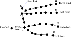
Figure 1: Schematic diagram of the Atlas robot’s kinematic tree. The links are the nodes and the joints are the edges. The link indices for certain key links are shown.

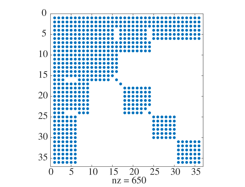
(a) Sparsity pattern of $M$.

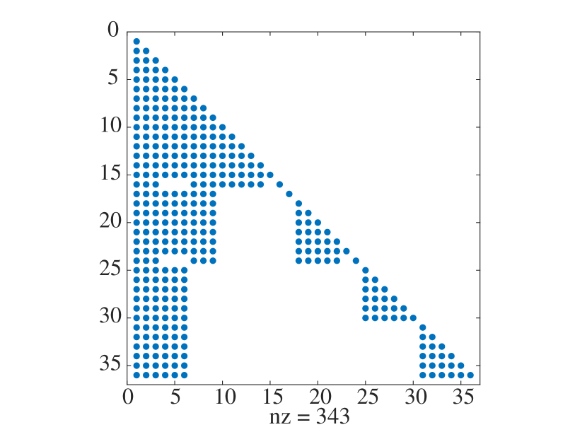
(b) Sparsity pattern of $L$.

(c) Sparsity pattern of $J$.

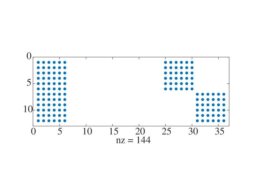
(d) Sparsity pattern of $Y$.

Figure 2: Sparsity pattern of various matrices in the LTL algorithm for an Atlas robot with a 6D weld constraint on each foot.

II-B Extended propagators

We now review the force and motion propagators used in propagation-based algorithms discussed later. Let $H_{i}^{A}$ denote the articulated body inertia (ABI) matrix [17], which is the apparent inertia of the $i$th link including the inertial contribution of all its descendant links. Projecting the ABI onto the $i$th joint’s motion subspace yields

$$D_{i}:=S_{i}^{T}H_{i}^{A}S_{i},$$ (7)

which is the $i$th link’s apparent inertia felt at the $i$th joint. Let

$$P_{i}:=(I_{6\times 6}-H_{i}^{A}S_{i}(D_{i})^{-1}S_{i}^{T}),$$ (8)

denote the projection matrix, that that transmits spatial forces acting on the $i$th link to its parent $\pi(i)$ after removing the force component that causes the $i$th joint’s motion. It is long known [21] that $P_{i}$’s transpose $P_{i}^{T}$ (also a projection matrix) is the motion propagator, that transmits accelerations acting on the parent link $\pi(i)$ to the child link $i$ through the $i$th joint.

By composing the force propagators, we obtain extended force propagators (EFP)

$${}^{j}P_{i}:=P_{\text{inter}(j,i)}\cdots P_{\pi(\pi(i))}P_{\pi(i)}P_{i},$$ (9)

that directly transmit spatial forces backward from the $i$th link to some ancestral $j$th link. Analogously, ${}^{j}P_{i}^{T}$ is the extended motion propagator (EMP) that transmits spatial accelerations forward from the $j$th link to the $i$th link. Trivially, ${}^{i}P_{i}=I_{6\times 6}$. Let

$${}^{\pi(i)}\Omega_{i}:=S_{i}(D_{i})^{-1}S_{i}^{T},$$ (10)

where ${{}^{\pi(i)}}\Omega_{i}\in\mathbb{R}^{6\times 6}$ denotes the apparent inverse spatial inertia. It maps forces acting on the $i$th link to the $i$th link’s accelerations due to the $i$th joint’s motion. The apparent inverse spatial inertia felt at the $i$th link due to the any joint $k\in\mathrm{anc}(i)$ can be obtained by backwardly transmitting the $i$th link’s forces using EFP, multiplying it with the $k$th link’s spatial inverse inertia and then forward propagating the resulting accelerations to the $i$th link using EMP. Accumulating these contributions for all the joints in $\mathrm{path}(i,j)$ gives

$$^{j}\Omega_{i}:=\sum_{k\in\text{path}(j,i)}{{}^{k}P}_{i}^{T}\ S_{k}(D_{k}^{-1})S_{k}^{T}\ {{}^{k}P_{i}},$$ (11)

where ${{}^{j}\Omega_{i}}$ is the apparent inverse inertia felt by forces acting on the $i$th link’s due to the motion of all joints $k\in\mathrm{path}(j,i)$.

To facilitate inverse OSIM computation, which is the constraint space inverse inertia, we introduce force and motion propagators in the constraint space. Let

$${}^{j}K_{i}^{A}:=K_{i}^{A}\ {{{}^{j}}P}_{i}^{T},$$ (12)

where, $K_{i}^{A}$ is the constraint space EMP (CEMP) that transmits the $i$th link’s spatial acceleration to the constraint space accelerations of all constraints on end effector links supported by the $i$th link denoted by $ES(i)$, ${}^{j}K_{i}^{A}\in\mathbb{R}^{m_{i}\times 6}$, is the CEMP that transmits $j$th link’s spatial accelerations ($j\in\text{anc(i)}$) to constraint space accelerations of the constraints supported by the $i$th link. Analogously, ${}^{j}K_{i}^{AT}$ is the constraint space EFP (CEFP), which backwardly transmits the constraint force magnitudes associated with the $i$th link’s supported constraints ($\bm{\lambda}^{A}_{i}$) to the spatial forces acting on the $j$th link due to these constraints. Using these terms, let

$${}^{k}L_{i,j}^{A}:=^{\text{cca}(i,j)}{K_{i}}^{A}\ {}^{k}\Omega_{\text{cca}(i,j)}\ ^{\text{cca}(i,j)}{K_{i}}^{AT},$$ (13)

where ${}^{k}L_{i,j}^{A}\in\mathbb{R}^{m_{i}\times m_{j}}$, is the cross-coupling constraint-space inverse inertia between the constraints on the $i$th and the $j$th links, considering the subtree rooted at the $k$th link ($k\in\mathrm{anc}(\mathrm{cca}(i,j))$). In other words, ${}^{k}L_{i,j}^{A}$ maps the $j$th link’s constraint force magnitudes $\bm{\lambda}^{A}_{j}$ to the $i$th link’s constraint space accelerations $K_{i}^{A}\mathbf{a}_{i}$ considering the subtree rooted at the $k$th link. Let

$$L_{k}^{A}:=\begin{bmatrix}{}^{k}L_{e_{1},e_{1}}^{A}&\ldots&{}^{k}L_{e_{1},e_{i}}^{A}&\ldots&{}^{k}L_{e_{1},e_{m}}^{A}\\ \vdots&\ddots&\vdots&\vdots&\vdots\\ {}^{k}L_{e_{1},e_{i}}^{AT}&\ldots&{}^{k}L_{e_{i},e_{i}}^{A}&\vdots&{}^{k}L_{e_{i},e_{m}}^{A}\\ \vdots&\ldots&\ldots&\ddots&\vdots\\ {}^{k}L_{e_{1},e_{m}}^{AT}&\ldots&{}^{k}L_{e_{i},e_{m}}^{AT}&\ldots&{}^{k}L_{e_{m},e_{m}}\end{bmatrix}$$ (14)

denote the constraint space inverse inertia of the subtree rooted at the $k$th link, by assembling the cross-coupling terms ${}^{k}L_{e_{i},e_{j}}^{A}\ \forall e_{i},e_{j}\in ES(k)$. The constraint space inverse inertia of the whole tree ($k=0$) gives the inverse OSIM

$$\Lambda^{-1}=L_{0}^{A}.$$ (15)

II-C PV-OSIM algorithm

Algorithm 1 lists the PV-OSIM [10] algorithm for completeness. The main computational bottleneck of PV-OSIM is the line 7 which requires $O(m^{2}d)$ number of operations, while line 6 requires $O(md)$ operations. All the other lines of the algorithm require $O(n)$ number of operations, bringing the total complexity to $O(n+m^{2}d)$.

Algorithm 1 The PV-OSIM algorithm

0:   $\mathbf{q^{p}}$,  $K_{i}$s,  robot model First forward sweep

1:  for $i$ in $\mathcal{S}$ do

2:     $K_{i}^{A}\leftarrow K_{i}$;  $L_{i}^{A}\leftarrow 0_{m_{i}\times m_{i}}\ H_{i}^{A}\leftarrow H_{i};$ Backward sweep

3:  for $i$ in $\mathcal{S}_{r}$ do

4:     $D_{i}=S_{i}^{T}H_{i}^{A}S_{i};\ P_{i}=(I_{6\times 6}-H_{i}^{A}S_{i}(D_{i})^{-1}S_{i}^{T})$

5:     $H_{\pi(i)}^{A}\leftarrow H_{\pi(i)}^{A}+P_{i}H_{i}^{A}$

6:     $K_{\pi(i)}^{A}\leftarrow\begin{bmatrix}K_{\pi(i)}^{A}\\ K_{i}^{A}P_{i}^{T}\end{bmatrix}$

7:     $L^{A}_{\pi(i)}\leftarrow\begin{bmatrix}L^{A}_{\pi(i)}&\\ &L^{A}_{i}+K_{i}^{A}S_{i}(D_{i})^{-1}S_{i}^{T}K_{i}^{AT}\end{bmatrix}$

8:  $\Lambda^{-1}=(L_{0}^{A})$

II-D Extended force propagator algorithm (EFPA)

Algorithm 2 presents the EFPA, whose recursive formulae are identical to PV-OSIM up to line 5. ${{}^{j}K}_{\pi(i)}^{A}$, which transmits the $\pi(i)$th link’s spatial acceleration to $j$th constraint’s space, is computed recursively in line 7. While it appears different from PV-OSIM’s line 6, these two lines are computationally identical. Only the EFPA maintains each end-effector’s CEMP separately for assembling the inverse OSIM later.

The fundamental difference between PV-OSIM and EFPA arises in line 10, where EFPA recursively computes $(^{0}\Omega_{i}{{}^{i}K}^{AT}_{j})\in\mathbb{R}^{6\times m_{j}}$, which maps the $j$th link’s constraint force magnitudes $\bm{\lambda}_{j}$ to $i$th link’s spatial acceleration $\mathbf{a}_{i}$ for each end-effector $j$ and all its ancestor links $i$. This requires $O(md)$ number of operations. Then each block of $\Lambda^{-1}$ is computed in line 12 using EFP, which requires a constant number of operations per block. This brings the total computational complexity of the algorithm to $O(n+md+m^{2})$.

Algorithm 2 The EFPA algorithm

0:   $\mathbf{q^{p}}$,  $K_{i}$s,  robot model First forward sweep

1:  for $i$ in $\mathcal{S}$ do

2:     $K_{i}^{A}\leftarrow K_{i}$;  $L_{i}^{A}\leftarrow 0_{m_{i}\times m_{i}}\ H_{i}^{A}\leftarrow H_{i};$ Backward sweep

3:  for $i$ in $\mathcal{S}_{r}$ do

4:     $D_{i}=S_{i}^{T}H_{i}^{A}S_{i};\ P_{i}=(I_{6\times 6}-H_{i}^{A}S_{i}(D_{i})^{-1}S_{i}^{T})$

5:     $H_{\pi(i)}^{A}\leftarrow H_{\pi(i)}^{A}+P_{i}H_{i}^{A}$

6:     for $j\in ES(i)$ do

7:        ${}^{j}K_{\pi(i)}^{A}={{}^{j}K}_{i}^{A}\ P_{i}^{T}$ Second forward sweep

8:  for $i\in\mathcal{S}$ do

9:     for $j\in ES(i)$ do

10:        $(^{0}\Omega_{i}{{}^{i}K}^{AT}_{j})=P_{i}^{T}(^{0}\Omega_{\pi(i)}{{}^{\pi(i)}K}^{AT}_{j})+^{\pi(i)}\Omega_{i}\ ^{i}K_{j}^{AT}$ Assembling the inverse OSIM

11:  for $i,j\in\mathcal{E}$, if $i\leq j$ do

12:     ${}^{0}L_{i,j}^{A}={{}^{i}K_{cca(i,j)}^{A}}(^{0}\Omega_{cca(i,j)}{{}^{cca(i,j)}K}^{A}_{j})$

III PV-OSIMr algorithm

Equipped with the notation from the previous section, we now adapt the PV-OSIM algorithm to obtain the PV-OSIMr algorithm. We first mention the insight that reduces PV-OSIM’s computational complexity and follow that with the PV-OSIMr presentation.

III-A Insight behind the reduced complexity result

The lines 6 of algorithm 1 which computes the CEFP requires $O(md)$ operations. However, if the total dimensionality of constraints supported by the $i$th link (number of rows in $K_{i}^{A}$) is more than six, one can simply compute the EFPs ${}^{j}P_{i}$ for $i$th link’s ancestors instead of the CEFPs, which requires only $O(d)$ operations. The CEFP can then be recovered from EFP using eq. 12.

Similarly, line 7 of algorithm 1 computes constraint space inverse inertia in $O(m^{2}d)$ operations. Instead, spatial inverse inertia ${{{}^{j}}\Omega}_{i}$ can be computed using the recursive version of eq. 11

$$^{\pi(k)}\Omega_{i}={{}^{k}\Omega_{i}}+{{}^{k}P}_{i}^{T}\ S_{k}(D_{k}^{-1})S_{k}^{T}\ {{}^{k}P_{i}},$$ (16)

in $O(d)$ operations. Each block ${}^{0}L_{i,j}^{A},\ \forall i,j\in\mathcal{E}$ of the inverse OSIM blocks can then be recovered using eq. 13

$$^{0}L_{i,j}^{A}=\ ^{\text{cca}(i,j)}K_{i}^{A}\ ({{}^{0}}\Omega_{\text{cca}(i,j)})\ ^{\text{cca}(i,j)}K_{j}^{AT},$$ (17)

in further $O(m^{2})$ operations. The equation above implies that the CEFP ${}^{\text{cca}(i,j)}K_{i}^{A}$ and the spatial inverse inertias $({{}^{0}}\Omega_{\text{cca}(i,j)})$ need to be computed only for the links that are $\mathrm{cca}(i,j),\forall i,j\in\mathcal{E}$, which is the same as the list $\mathcal{N}$.

III-B Algorithmic form

To capitalize on the insights described in section III-A, we modify the PV-OSIM’s backward sweep (see algorithm 1) to recursively compute only the EFP ${}^{\mathcal{N}\mathrm{anc}(j)}P_{j}^{A}$ and inverse inertia ${}^{\mathcal{N}\mathrm{anc}(j)}\Omega_{j}^{A}$ between a link $j\in\mathcal{N}$ and its immediate ancestor link in $\mathcal{N}$, given by $\mathcal{N}\mathrm{anc}(j)$. This way, we propagate fixed size matrices backward in the backward sweep unlike the PV-OSIM algorithm where the matrix sizes grow with the number of constraints. At the end of the sweep we obtain the terms ${}^{\mathcal{N}\text{anc}(j)}\Omega_{j}$ and ${}^{\mathcal{N}\text{anc}(j)}P_{j}$ for every $j\in\mathcal{N}$.

Then, in a limited forward sweep over only the links in $\mathcal{N}$, the inverse inertia terms ${}^{0}\Omega_{j},\ \forall j\in\mathcal{N}$ is computed using eq. 16

$$^{0}\Omega_{j}={{}^{\mathcal{N}\text{anc}(j)}\Omega_{j}}+{{}^{\mathcal{N}\text{anc}(j)}P}_{j}^{T}\ {}^{0}\Omega_{\mathcal{N}\text{anc}(j)}\ {{}^{\mathcal{N}\text{anc}(j)}P_{j}}.$$ (18)

Then, in a limited backward sweep, the CEMP for every end-effector $e_{i}\in\mathcal{E}$ is computed recursively over only the links in $\mathcal{N}\cap\mathrm{cca}(e_{i})$, using eq. 12

$${}^{\mathcal{N}\text{anc}(j)}K_{e_{i}}=\ ^{j}K_{e_{i}}\ {{}^{\mathcal{N}\text{anc}(j)}P}_{j}^{T}.$$ (19)

This gives us all the necessary terms to assemble the inverse OSIM matrix in eq. 14 using eq. 17. The full algorithm is presented in algorithm 3

Algorithm 3 The PV-OSIMr algorithm

0:   $\mathbf{q^{p}}$,  $K_{i}$s,  robot model First forward sweep

1:  for $i$ in $\mathcal{S}$ do

2:     $H_{i}^{A}\leftarrow H_{i};$

3:     if $i\in\mathcal{E}$ and $i\notin\mathcal{N}$ then

4:        ${}^{i}P_{i}=K_{i}$;  ${}^{i}\Omega_{i}^{A}\leftarrow 0_{m_{i}\times m_{i}};\ d(i)\leftarrow i$ Backward sweep

5:  for $i$ in $\mathcal{S}_{r}$ do

6:     if $i\in\mathcal{N}$ then

7:        $d(i)\leftarrow i;\ ^{i}P_{i}=I_{6\times 6};\ ^{i}\Omega_{i}^{A}\leftarrow 0_{6\times 6}$

8:     $D_{i}=S_{i}^{T}H_{i}^{A}S_{i};\ P_{i}=(I_{6\times 6}-H_{i}^{A}S_{i}(D_{i})^{-1}S_{i}^{T})$

9:     $H_{\pi(i)}^{A}\leftarrow H_{\pi(i)}^{A}+P_{i}H_{i}^{A};$ ${{}^{\pi(i)}P_{d(i)}}=P_{i}\ ^{i}P_{d(i)}$

10:     ${}^{\pi(i)}\Omega_{d(i)}={{}^{i}\Omega_{d(i)}}+{{}^{i}P}_{d(i)}^{T}\ S_{i}(D_{i}^{-1})S_{i}^{T}\ {{}^{i}P_{d(i)}}$

11:     d($\pi(i)$) $\leftarrow d(i)$ Limited forward sweep over $\mathcal{N}$

12:  for $i$ in $\mathcal{N}$ do

13:     ${}^{0}\Omega_{i}={{}^{\mathcal{N}\text{anc}(i)}\Omega_{i}}+{{}^{\mathcal{N}\text{anc}(i)}P}_{i}^{T}\ {}^{0}\Omega_{\mathcal{N}\text{anc}(i)}\ {{}^{\mathcal{N}\text{anc}(i)}P_{i}}$ Limited backward sweep over $\mathcal{N}$

14:  for $e_{i}\in\mathcal{E}$ do

15:     for $i$ in $\mathcal{N}_{r}\cap\text{anc}(e_{i})$ do

16:        ${}^{\mathcal{N}\text{anc}(i)}K_{e_{i}}=\ ^{i}K_{e_{i}}\ {{}^{\mathcal{N}\text{anc}(i)}P}_{i}^{T}$ Assemble inverse OSIM matrix

17:  for $i,j\in\mathcal{E}$ if $i\leq j$ do

18:     ${}^{0}L_{i,j}^{A}=\ ^{\text{cca}(i,j)}K_{i}^{A}\ ({{}^{0}}\Omega_{\text{cca}(i,j)})\ ^{\text{cca}(i,j)}K_{j}^{AT}$

19:     if $i\neq j$ then

20:        ${}^{0}L_{j,i}^{A}=^{0}L_{j,i}^{AT}$

III-B1 Complexity analysis

We now analyze the asymptotic computational complexity of algorithm 3. All the computations performed from line 2 to line 13 in algorithm 3 require a fixed number of operations and are performed at most $n$ times and therefore require $O(n)$ operations. Line 18 also requires a fixed number of operations and is performed $m^{2}$ times, thus requiring $O(m^{2})$ operations.

The CEFP computation in line 16 for an end-effector $e_{i}$ is performed at most $m$ times in the worst case, which occurs when there is a unique closest common ancestor for $e_{i}$ and all other end-effectors. The line 16 requires $O(1)$ operations each time, therefore its complexity for all end-effectors is upper-bounded by $O(m^{2})$. This brings the total complexity of the PV-OSIMr algorithm to $O(n+m^{2})$.

IV Results and discussions

IV-A Implementation

Similarly to [10], we have implemented the PV-OSIMr algorithm using the CasADi [22] library. Apart from enabling efficient C code generation for the dynamics algorithms, CasADi implementation enables us to count the number of operations in a given algorithm. We will use this operation count to benchmark PV-OSIMr with our implementation of PV-OSIM, EFPA and LTL-OSIM algorithms. The algorithms presented in this paper assumed that all the quantities are expressed in an inertial frame to avoid the clutter due to spatial transforms. However, the OSIM algorithms (as well as the ABA algorithm [2], [23]) are more efficiently implemented in the local frame. Therefore, our CasADi implementation is also in the local frame. Readers are referred to the source code of the implementation for further details on the local frame implementation. A C++ version of PV-OSIMr has also been implemented in the Pinocchio library [15], which will be released upon the acceptance of this letter.

IV-B Computational scaling study

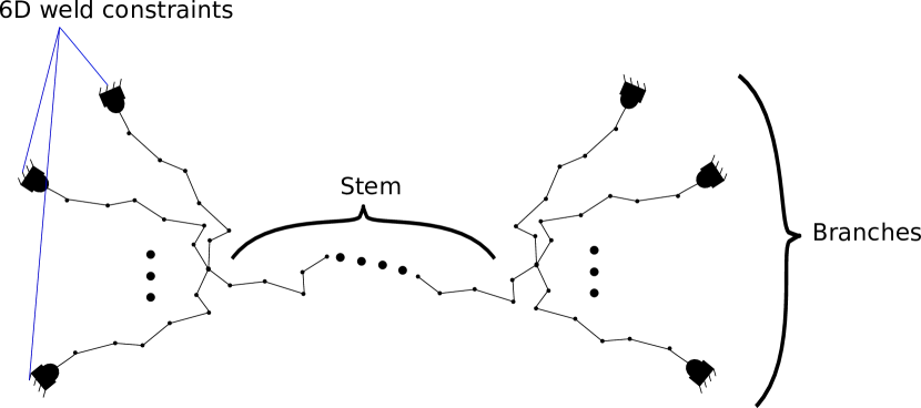
(a) The mechanism on which the OSIM scaling is benchmarked.

(b) One branch on each side (a chain structure).

(c) Two branches on either side.

(d) Four branches on either side.

(e) Seven branches on either side.

(f) Ten branches on either side.

Figure 3: Benchmarking the number of operations of the different OSIM algorithms.

We now analyze the computational scaling of the low-complexity OSIM algorithms (PV-OSIM, EFPA and PV-OSIMr) w.r.t. both increasing tree depth, and number of branches and constraints. Consider a mechanism (see fig. 3(a)) with a long stem and branches on either side. Each branch tip is rigidly constrained with a weld constraint (6D constraint). This mechanism is chosen because the path depth along which the constraints are propagated increases linearly with the number of stem links for any choice of floating base link. The operation count of the different algorithms for mechanisms with different number of branches is plotted in fig. 3, with the x-axis of each plot showing the stem length.

For a single branch, the mechanism is a serial chain with 6D constraints on each end, and there is no difference between the PV-OSIMr and PV-OSIM algorithms as the dimensionality of the propagated constraints does not exceed 6 to benefit from PV-OSIMr’s optimization w.r.t to PV-OSIM. For two or more branches, PV-OSIMr’s advantage becomes apparent as it scales significantly more gently than the PV-OSIM algorithm due to its lower computational complexity. The EFPA is more expensive than both the PV-OSIMr and the PV-OSIM for nearly all the considered mechanisms. As discussed extensively in [10], despite having a lower asymptotic complexity than PV-OSIM, EFPA is more expensive for small mechanisms with few constraints ($<\sim 50$) because it has a three sweep structure compared to the two sweep structure of PV-OSIM, and it computes inverse inertia in each link’s frame (see line 10 in algorithm 2) which requires an expensive similarity transformation during the second forward sweep.

However, for long enough mechanisms with sufficiently many constraints the EFPA eventually becomes faster than the PV-OSIM (see fig. 3(f)) due to its lower computational complexity. Finally, we note that PV-OSIMr was more efficient than both PV-OSIM and EFPA, which are the state-of-the-art inverse OSIM algorithms.

IV-C Humanoid robot standing constraints

(a) 6D constraint on each foot.

(b) 12D constraint on each foot.

Figure 4: Comparing the number of computation operations of the OSIM algorithms for the Atlas robot.

We now compare the different OSIM algorithms (PV-OSIMr, PV-OSIM, EFPA and LTL) for a humanoid robot Atlas and the results are tabulated in fig. 4. The number of operations required to compute the inverse OSIM when the Atlas robot is standing, which is modeled as each of its feet being rigidly connected to the world with a 6D weld constraint is plotted in fig. 4(a). The hip link to which both the legs are connected is selected as the floating base. There is no difference between PV-OSIM and PV-OSIMr in this case as the two 6D constraints meet only at the floating-base link during the backward propagation and therefore does not benefit from the PV-OSIMr’s improvement.

Next, we consider the example where the foot-ground constraint is modelled as connect-type 3D constraints at four contact points as is commonly done in simulators [24]. PV-OSIM propagates 12D constraints from each foot while PV-OSIMr only propagates 6D constraints leading to a significant improvement in computational expense with PV-OSIM requiring 19.9% more operations relative to the PV-OSIMr algorithm. For both examples, the PV-OSIM and PV-OSIMr were significantly more efficient than the EFPA and the LTL algorithms.

IV-D Humanoid robot with shadow hands

(a) Considering a single shadow hand, a 24 d.o.f system. Connect constraint (3D) on each fingertip leading to 15 constraints.

(b) Shadow hand connected to Atlas’s left wrist with same constraint as in fig. 5(a) (total 15 constraints on a 60 d.o.f system).

(c) Shadow hand connected to both wrists of Atlas with each hand having the same constraints as in fig. 5(a) (total 30 constraints on an 84 d.o.f system).

(d) Atlas with both hands constrained as in fig. 5(c) along with 6D weld constraint on each foot for standing. (total 42 constraints on an 84 d.o.f system).

Figure 5: Comparing the number of computation operations of the OSIM algorithms for the Atlas robot equipped with the shadow hand.

Finally, we compare the OSIM algorithms for an Atlas robot equipped with the Shadow hand in fig. 5. We impose a 3D connect type constraint on each fingertip of the hand leading to a total of 15D constraints. We plot the OSIM results for i) just a single Shadow hand, ii) an Atlas robot with a single shadow hand connected to its left wrist, iii) an Atlas robot with a shadow hand connected to each wrist, and iv) finally an Atlas robot with both its feet constrained with 6D weld constraints on each foot in addition to the 15D constraint on each shadow hand in fig. 5(a), fig. 5(b), fig. 5(c) and fig. 5(d) respectively.

The typically expensive LTL-OSIM is computationally more efficient than EFPA for just the Shadow Hand in fig. 5(a) because the LTL-OSIM benefits from the sparsity induced by the extensive branching of the hand’s mechanism. When the Shadow hand is connected to the Atlas robot in the remaining three examples, the performance of the high complexity LTL-OSIM significantly deteriorates compared to the lower complexity algorithms PV-OSIMr, PV-OSIM and EFPA. The PV-OSIMr algorithm is found to be significantly more efficient than the other algorithms with up to $\sim$34% fewer operations needed than the next most efficient algorithm PV-OSIM.

IV-E Caveats

While PV-OSIMr outperforms PV-OSIM in all the examples presented so far, we note that there were some cases when PV-OSIM was more efficient. This occurs especially when more than six constraints need to be propagated in PV-OSIM through only a few ($\leq 3$) single d.o.f. joints, because for single d.o.f. joints PV-OSIM recursively computes the OSIM through efficient symmetric rank-1 (SR1) updates per joint (by computing the vector $K_{i}^{A}S_{i}$, see line 7 in algorithm 1). PV-OSIMr instead performs two symmetric rank-6 computations (see line 18 and line 13 in algorithm 3), which have are more expensive than SR1 updates over a few joints. For example, if a 6D weld constraint is imposed on both the hands (without the Shadow Hand) in addition to the 6D constraints on the feet of Atlas considered in section IV-C, the PV-OSIM requires $\sim$1.5% fewer operations than PV-OSIMr, because PV-OSIMr’s improved backward over just three joints (from sternum to the floating base hip link) does not compensate the aforementioned overhead of PV-OSIMr.

V Conclusions

We presented PV-OSIMr, an algorithm with the lowest known computational complexity of $O(n+m^{2})$ to compute the Delassus matrix or the inverse OSIM matrix, which is a fundamental quantity with various simulation and control applications in a computationally demanding setting. Our algorithm is derived by optimizing the computational ordering of the PV-OSIM algorithm that avoids propagating constraints of more than six dimensions. The PV-OSIMr algorithm not only has the lowest computational complexity, but is also found to lead to up to 24% improvement over practical examples involving the Atlas robot. Furthermore, since computing the inverse OSIM matrix requires considering all the $n$ joints and populating a dense matrix of size $m\times m$, the achieved computational complexity of $O(n+m^{2})$ can be considered to be asymptotically optimal.

References

- [1] Bernard Brogliato. Nonsmooth Mechanics: Models, Dynamics and Control. Springer, 2016.
- [2] Roy Featherstone. Rigid body dynamics algorithms. Springer, 2014.
- [3] Justin Carpentier, Rohan Budhiraja, and Nicolas Mansard. Proximal and sparse resolution of constrained dynamic equations. In Robotics: Science and Systems 2021, 2021.
- [4] Martin L Felis. Rbdl: an efficient rigid-body dynamics library using recursive algorithms. Autonomous Robots, 41(2):495–511, 2017.
- [5] Jemin Hwangbo, Joonho Lee, and Marco Hutter. Per-contact iteration method for solving contact dynamics. IEEE Robotics and Automation Letters, 3(2):895–902, 2018.
- [6] Oussama Khatib. A unified approach for motion and force control of robot manipulators: The operational-space formulation. IEEE Journal on Robotics and Automation, 3(1):43–53, 1987.
- [7] Alexander Dietrich, Christian Ott, and Alin Albu-Schäffer. An overview of null space projections for redundant, torque-controlled robots. 34(11):1385–1400, 2015.
- [8] Ludovic Righetti, Jonas Buchli, Michael Mistry, Mrinal Kalakrishnan, and Stefan Schaal. Optimal distribution of contact forces with inverse-dynamics control. The International Journal of Robotics Research, 32(3):280–298, 2013.
- [9] Étienne Delassus. Mémoire sur la théorie des liaisons finies unilatérales. In Annales scientifiques de l’École normale supérieure, volume 34, pages 95–179, 1917.
- [10] Ajay Suresha Sathya, Herman Bruyninckx, Wilm Decre, and Goele Pipeleers. An Efficient Constrained Dynamics Algorithm based on an Equivalent LQR Formulation using Gauss’ Principle of Least Constraint. October 2022.
- [11] Kenneth Kreutz-Delgado, Abhinandan Jain, and Guillermo Rodriguez. Recursive formulation of operational-space control. The International journal of robotics research, 11(4):320–328, 1992.
- [12] Kyong-Sok Chang and Oussama Khatib. Efficient recursive algorithm for the operational space inertia matrix of branching mechanisms. Advanced Robotics, 14(8):703–715, 2001.
- [13] Patrick Wensing, Roy Featherstone, and David E Orin. A reduced-order recursive algorithm for the computation of the operational-space inertia matrix. In 2012 IEEE International Conference on Robotics and Automation, pages 4911–4917. IEEE, 2012.
- [14] Roy Featherstone. Exploiting sparsity in operational-space dynamics. The International Journal of Robotics Research, 29(10):1353–1368, 2010.
- [15] Justin Carpentier, Guilhem Saurel, Gabriele Buondonno, Joseph Mirabel, Florent Lamiraux, Olivier Stasse, and Nicolas Mansard. The pinocchio c++ library: A fast and flexible implementation of rigid body dynamics algorithms and their analytical derivatives. In 2019 IEEE/SICE International Symposium on System Integration (SII), pages 614–619. IEEE, 2019.
- [16] AF Vereshchagin. Computer simulation of the dynamics of complicated mechanisms of robot-manipulators. Eng. Cybernet., 12:65–70, 1974.
- [17] Roy Featherstone. The calculation of robot dynamics using articulated-body inertias. The international journal of robotics research, 2(1):13–30, 1983.
- [18] Anatolii Fedorovich Vereshchagin. Modeling and control of motion of manipulational robots. Soviet Journal of Computer and Systems Sciences, 27(5):29–38, 1989.
- [19] Je P Popov, Anatolij Fedorovič Vereshchagin, and Stanislav Leonidovič Zenkevič. Manipuljacionnyje roboty: Dinamika i algoritmy. Nauka, 1978.
- [20] Roy Featherstone. Efficient factorization of the joint-space inertia matrix for branched kinematic trees. The International Journal of Robotics Research, 24(6):487–500, 2005.
- [21] Kathryn Weed Lilly. Efficient dynamic simulation of multiple chain robotic systems. The Ohio State University, 1989.
- [22] Joel AE Andersson, Joris Gillis, Greg Horn, James B Rawlings, and Moritz Diehl. Casadi: a software framework for nonlinear optimization and optimal control. Mathematical Programming Computation, 11(1):1–36, 2019.
- [23] M Otter, H Brandl, and R Johanni. An algorithm for the simulation of multibody systems with kinematic loops. In Proceedings of the 7th World Congress on Theory of Machines and Mechanisms, IFToMM, Sevilla, Spain, 1987.
- [24] Stéphane Caron, Quang-Cuong Pham, and Yoshihiko Nakamura. Stability of surface contacts for humanoid robots: Closed-form formulae of the contact wrench cone for rectangular support areas. In 2015 IEEE International Conference on Robotics and Automation (ICRA), pages 5107–5112. IEEE, 2015.