Robustness-Guided Image Synthesis for Data-Free Quantization

Abstract

Quantization has emerged as a promising direction for model compression. Recently, data-free quantization has been widely studied as a promising method to avoid privacy concerns, which synthesizes images as an alternative to real training data. Existing methods use classification loss to ensure the reliability of the synthesized images. Unfortunately, even if these images are well-classified by the pre-trained model, they still suffer from low semantics and homogenization issues. Intuitively, these low-semantic images are sensitive to perturbations, and the pre-trained model tends to have inconsistent output when the generator synthesizes an image with poor semantics. To this end, we propose Robustness-Guided Image Synthesis (RIS), a simple but effective method to enrich the semantics of synthetic images and improve image diversity, further boosting the performance of downstream data-free compression tasks. Concretely, we first introduce perturbations on input and model weight, then define the inconsistency metrics at feature and prediction levels before and after perturbations. On the basis of inconsistency on two levels, we design a robustness optimization objective to enhance the semantics of synthetic images. Moreover, we also make our approach diversity-aware by forcing the generator to synthesize images with small correlations in the label space. With RIS, we achieve state-of-the-art performance for various settings on data-free quantization and can be extended to other data-free compression tasks.

Introduction

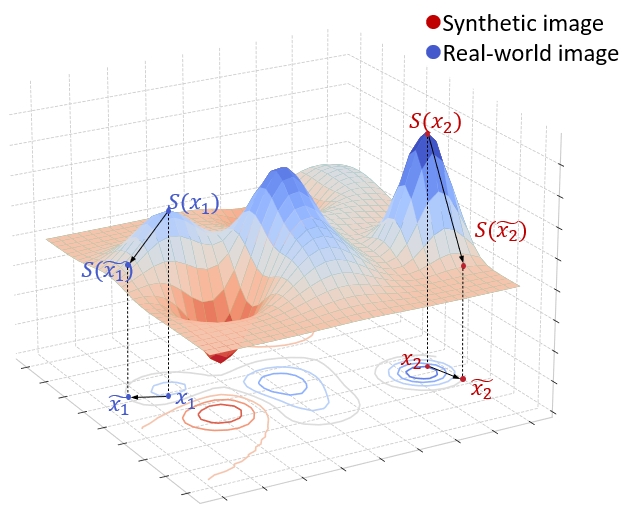
Figure 1: Visualization of the loss landscape. Note that we reverse the y-axis for visual convenience.

Recently, deep neural networks have achieved great accomplishment in many areas, including computer vision (He et al. 2016; Girshick 2015; Sandler et al. 2018) and natural language processing (Zia and Zahid 2019; Mikolov et al. 2010; Devlin et al. 2018). Despite their satisfactory performance, the huge number of parameters and high computational cost prevent them from being deployed to edge computing devices. Quantization, which converts parameters from full-precision to low-precision, has become a promising method for model compression. A large number of methods (Liu et al. 2020, 2018; Fan et al. 2020; Zhuang et al. 2018) minimize the quantization error through training data and achieve great performance in low-bit quantization. However, accessibility to the original training data during the quantization process is not always possible due to privacy and security reasons, especially in medical and industrial scenarios. Data-driven methods would fail in this case.

Therefore, data-free quantization has been proposed for compression under privacy protection. Among some excellent works (Nagel et al. 2019; Banner et al. 2018; Cai et al. 2020; Nagel et al. 2019), generative methods (Choi et al. 2021; Xu et al. 2020; Zhu et al. 2021; Choi et al. 2022; Qian et al. 2023b, a; Li et al. 2023; Shang et al. 2023; Choi et al. 2020) have drawn much attention due to their great performance. These methods synthesize fake data through generators and use them to calibrate or fine-tune the quantified model. Hence, the quality of synthesized images influences the quantization performance greatly.

Beyond various image priors (e.g., match BN statistics (Cai et al. 2020)) being used during image synthesis, most of the existing methods feed the synthesized images to the pre-trained model, then minimize the cross-entropy loss to guarantee the semantics of images (Xu et al. 2020; Zhang et al. 2021). Nevertheless, even if the images are well-classified, they still suffer from low semantics, limiting the performance of downstream model compression tasks. The phenomenon can be explained in two aspects. On one hand, studies (Goodfellow, Shlens, and Szegedy 2014a; Moosavi-Dezfooli, Fawzi, and Frossard 2016) in model attack show that deep neural networks can be easily misled by adding adversarial perturbations. Therefore, it is unsurprising that the pre-trained model has high confidence in these noise-like data. On the other, the lack of a discriminator in data-free scenarios greatly limits the performance of the generator, and it only needs to match the image and class priors, but ignores the semantics of synthesized images. As a result, classification loss is insufficient to guide the generator in synthesizing samples with high semantics.

To this end, we manage to enrich the semantics of synthetic images in our work. Our intuition is that the low-quality images synthesized by existing methods are easily hampered, while real-world data are more robust towards perturbations due to their rich semantic information. In other words, the pre-trained model tends to have consistent representation and prediction which may not be easily disturbed for semantically abundant images (e.g., real-world data). To verify our hypothesis, we conduct a motivational experiment, as shown in Fig. 1. Concretely, we visualize the loss landscape of GDFQ (Xu et al. 2020), one of the SOTA methods in data-free quantization, and we plot the training data (real-world image) and synthesized image on the loss landscape as $\bm{x}_{1}$ and $\bm{x}_{2}$ respectively. Then, we apply input and weight perturbations to both images and denote the disturbed images as $\tilde{\bm{x}}_{1}$ and $\tilde{\bm{x}}_{2}$. It’s observed that the real-world image has a relatively smooth neighborhood in the loss landscape, while the loss of synthetic image changes dramatically nearby, implying the representation or prediction could have a large discrepancy before and after perturbations.

Based on the above observation, we propose a simple but effective method called Robustness-Guided Image Synthesis (RIS) to enrich the semantics of synthesized images, and further boost downstream data-free model compression tasks.

Concretely, we first conduct motivational experiments to verify that these low semantic images synthesized by existing methods are sensitive toward perturbations, which is different from real data with rich semantic information. Then, we explicitly model the inconsistency at feature and prediction levels before and after different kinds of perturbations as image robustness, and further design a robustness optimization objective for training the generator. The proposed robustness loss significantly improves the semantics of the synthetic images by forcing a smooth neighborhood in the loss landscape, as visualized in Fig. 1. On the other, we also alleviate the image homogenization problem (Zhang et al. 2021) via formulating an optimization problem and replacing the ont-hot label set with multiple soft labels with minimal correlation. With RIS, the Fréchet Inception Distance (FID) (Heusel et al. 2017) and Inception Score (IS) (Salimans et al. 2016) of synthetic images outperform the baseline with an improvement of 80.13 and 22.44 on ImageNet (Krizhevsky, Sutskever, and Hinton 2012).

Experiments on a variety of pre-trained models and datasets show RIS consistently achieves significant performance improvement. Moreover, our method is not limited to quantization, which can be extended to other data-free scenarios such as data-free knowledge distillation (Hinton et al. 2015).

We make the following major contributions. 1) We identify that the images synthesized by existing methods are more sensitive toward perturbations than natural images, leading to the low-semantic and limiting the performance of downstream tasks. 2) We propose the Robustness-Guided Image Synthesis (RIS) scheme, a simple but effective method to enrich the semantics and improve the diversity of synthetic images. 3) We conduct extensive experiments, showing that the proposed RIS outperforms various existing data-free quantization methods by a large margin, and can be further extended to data-free knowledge distillation.

Related Work

Data-Free Model Compression

Knowledge Distillation Early works in data-free scenarios focus on knowledge distillation (Hinton et al. 2015), which devise different regularizations for learning image priors (Lopes, Fenu, and Starner 2017; Nayak et al. 2019; Zhu, Hong, and Zhou 2021; Yu et al. 2023; Binici et al. 2022; Hao et al. 2022). They can be roughly divided into three categories: 1) synthesis from noise. Lopes et al. (Lopes, Fenu, and Starner 2017) utilize the activation records (i.e., means and covariance), which are restored as metadata for reconstructing training data. Nayak et al. (Nayak et al. 2019) model the softmax space of the teacher as a Dirichlet distribution and craft data from the parameters of the teacher. DeepInversion (Yin et al. 2020) combines the image prior presented by (Mordvintsev, Olah, and Tyka 2015) and aligns the BN statistics of the real ones. Although these methods can obtain high semantic images, it has the drawback of huge computational costs because each batch of synthetic images has to optimize from the beginning. 2) reconstruction with a generator. Represented by DAFL (Chen et al. 2019), these methods synthesize images from a generator. DAFL exploits cross-entropy loss as the class prior and maximum activation as the semantic prior. Luo et al. (Luo et al. 2020) use multi-generators and further extend to the large-scale dataset i.e. ImageNet (Krizhevsky, Sutskever, and Hinton 2012). 3) adversarial exploration. ZSKT (Micaelli and Storkey 2019) and DFAD (Fang et al. 2019) train an adversarial generator to search for images where the prediction of the student poorly matches the teacher’s prediction. However, these methods are sensitive to hyperparameters.

Quantization Most data-free quantization methods share a similar pipeline with data-free knowledge distillation: first synthesize images, then utilize them as surrogates for the original training data. ZeroQ (Cai et al. 2020), as the pioneer of the generative method for quantization, synthesizes data that match the statistics of BN (Ioffe and Szegedy 2015) layers. GDFQ (Xu et al. 2020) further uses the cross-entropy loss to ensure the synthesized images can be classified by the pre-trained network correctly. Based on the GDFQ framework, DSG (Zhang et al. 2021) optimizes the diversity of synthesized images by relaxing BN statistics constraint, while Qimera (Choi et al. 2021) focuses on generating samples nearing the classification boundary by using superposed latent embeddings. AutoReCon (Zhu et al. 2021) first searches for an optimized neural architecture to reconstruct the generator. AIT (Choi et al. 2022) argues that the classification loss and KL divergence have gradient confliction thus excluding the cross-entropy loss and proposes gradient inundation to solve infrequent updates of the quantized model. IntraQ (Zhong et al. 2022) imitates real data by generating heterogeneous synthetic images. HAST (Li et al. 2023) solves real data degradation by synthesizing hard samples and further promoting sample difficulty while training models. AdaSG (Qian et al. 2023b) enhances image adaptability while ensuring model accuracy by rethinking data-free quantization as a zero-sum game between the generator and the quantized network. AdaDFQ (Qian et al. 2023a) further improves it by optimizing the margin between the lower and upper boundaries defined by disagreement and agreement samples. These approaches consider the distribution of synthesized data at the statistical level but ignore the critical issue of generation quality. All these methods suffer from synthesizing unrealistic images with low semantics.

Image Robustness

Robustness (Box 1979) is defined as the property of a procedure that renders the answers it gives insensitivity to departures, which is used to describe systems, models, or images. Image robustness (Meer 2004; Vacavant 2016) is a concept in signal processing that means the image still has a certain degree of fidelity after various signal processing or attacks. In the field of watermarking, a group of methods design robust watermarks to resist the transformations of images (Cox et al. 1996). Image steganography communicates secret data by adding undetectability and robustness signal to the original image (Cheddad et al. 2010). In model defense (Papernot et al. 2016), a few methods exploit the prediction inconsistency to detect adversarial examples (Xu, Evans, and Qi 2017; Meng and Chen 2017; Feinman et al. 2017), which share the same spirits with our work. Xu et al. (Xu, Evans, and Qi 2017) introduce pre-processing the input images, then calculating the prediction shift score to separate adversarial samples from the natural ones. In this paper, we also transform the images and make use of the inconsistency. The biggest difference is that we explicitly model the robustness at feature and prediction levels, and use it as a guidance for image synthesis.

Method

Generative Data-Free Quantization

Generative data-free quantization methods, pioneered by (Xu et al. 2020), have drawn great attention due to their excellent performance and efficiency, which employ a generator $G$ to fit real training data distribution. With synthesized data, the quantized model is fine-tuned by mimicking the behavior of the pre-trained model $\mathcal{M}$ through knowledge distillation. Take GDFQ (Xu et al. 2020) as an example, the generator synthesize fake data $\bm{x}$ from the Gaussian noise z, conditional on the one-hot label $y$:

$$\bm{x}=G(\textbf{z}\mid y),\qquad\textbf{z}\sim\mathcal{N}(0,1)$$ (1)

The generated image is then classified by the pre-trained model $\mathcal{M}$, which is composed of a feature extractor $f$ and a classifier $g$, and update the generator by the classification loss:

$$\mathcal{L}_{\text{CE}}(G)=\mathbb{E}_{\textbf{z},y}\left[\mathrm{CE}(g(f(\bm{x})),y)\right],$$ (2)

Meanwhile, mean square error (MSE) loss is used to align the mean and variance at BN layers:

$$\mathcal{L}_{\text{BNS}}(G)=\sum_{l=1}^{L}\|{\bm{\mu}_{l}^{r}-\bm{\mu}_{l}}\|_{2}^{2}+\|{\bm{\sigma}_{l}^{r}-\bm{\sigma}_{l}}\|_{2}^{2},$$ (3)

where $\mu_{l}^{r}$ and $\sigma_{l}^{r}$ refer to the mean and variance of the synthesized images at the $l$-th BN layer, $\mu_{l}$ and $\sigma_{l}$ is the mean and variance stored in the pre-trained model. The overall objective for generator $G$ is:

$$\mathcal{L}_{\text{GDFQ}}(G)=\mathcal{L}_{\text{CE}}(G)+\alpha\mathcal{L}_{\text{BNS}}(G).$$ (4)

Based on the GDFQ framework, a few methods attempt to improve the quality of generated data from different aspects. DSG (Zhang et al. 2021), which aims to improve the diversity of synthesized images, modifies $\mathcal{L}_{BNS}(G)$ term by adding slack variables and designing layerwise sample enhancement. While Qimera (Choi et al. 2021) considers images near the decision boundary to be more helpful for data-free quantization. These approaches improve the samples at the distribution level, but ignore the critical point —the semantic and quality of synthesized images.

Semantic Enhancement with Input and Weight Perturbations

In this section, we delve into enhancing the semantic information of the synthetic images and further boosting the performance of data-free model compression tasks (e.g., quantization). Concretely, we first propose to involve perturbations on both input and weight levels, then explicitly define a robustness metric via the model inconsistency on feature representation and predicted distribution after perturbations. Finally, we design an additional optimization objective for supervising the generator based on the robustness metric.

Perturbations on Input and Model Weight

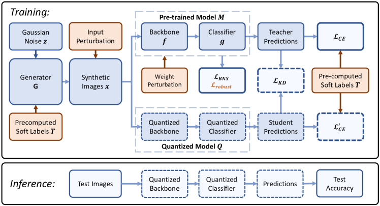
Figure 2: The pipeline of RIS. The solid line boxes refer to the teacher (pre-trained) model and losses for updating the generator $G$, while the dashed line boxes are the quantized model and its loss function. Proposed components are denoted as orange.

Recall in Fig. 1, we verify that low semantic images are more sensitive towards perturbations. Hence, our core idea is to explicitly optimize the generator to synthesize images that the teacher model has consistent outputs before or after the perturbations. To this end, the first step of our method is to introduce perturbations from input and model weight. For input perturbation, we implement it with several data augmentation strategies. As shown in Figure 2, the original images $\bm{x}$ as well as the augmented ones $\mathcal{A}(\bm{x})$ are fed into the full-precision (teacher) model and we optimize the generator with a consistency loss which will introduce in the following sections. It’s worth noting that input perturbations can be instantiated as any differentiable data augmentation method (see Appendix for details).

On the other, we further introduce perturbation on weight as complementary. Given the teacher model $({g}\circ f)$ with parameters $\bm{w}$, we add a perturbation term $\bm{v}$ to the original weight, i.e., $\bm{w}^{\prime}=\bm{w}+\bm{v}$. As shown in Figure 2, we explore three different weight perturbation strategies: a), we instantiate the perturbation term as the Gaussian noise with mean $\mu$ and deviation $\sigma$: $\bm{v}\sim\mathcal{N}(\mu,\sigma^{2})$; b), we conduct experiments with adversarial weight perturbation (similar with several studies in model defense (Goodfellow, Shlens, and Szegedy 2014b; Madry et al. 2018; Wu, Xia, and Wang 2020)), i.e., $\bm{v}=\gamma\,\frac{\nabla_{w}\mathrm{CE}[(g\circ f)_{w}(\bm{x}_{i}),y]}{\nabla_{w}\|\mathrm{CE}[(g\circ f)_{w}(\bm{x}_{i}),y]\|}\,\|\bm{w}\|$, which is also shown as effective in experiments; c), Dropout (Srivastava et al. 2014) as a widely-used technique to enhance model generalization and reducing overfitting, can also regard as a weight perturbation strategy where $\bm{v}$ is $-\bm{w}$ for discarded neurons and zero for others.

Robustness Modeling via Inconsistency

In this section, we explicitly model image robustness by the maximum value of inconsistency at the level of feature and prediction after $n$ perturbations. At the feature level, we exploit the cosine distance to measure the variation of features:

$${\mathcal{R}_{f}(\bm{x})=\max\limits_{1\leq i\leq n}\frac{\left<f(\bm{x}),\mathcal{A}_{i}(f(\bm{x}))\right>}{\|f(\bm{x})\|\cdot\|\mathcal{A}_{i}(f(\bm{x}))\|}},$$ (5)

where $\bm{x}$ refers to the synthesized image, $\mathcal{A}_{i}$ is the $i$-th different perturbation strategy, $f(\cdot)$ denotes the operation of extracting the features in the pre-training model, and $\mathcal{R}_{f}(\bm{x})$ denotes the inconsistency of the synthetic image $\bm{x}$ on feature level. Since the details or textures of the synthetic image may not be held after perturbations, we utilize the feature embedding of the last layer which indicates the high-level semantics (should be consistent towards perturbations).

At the prediction level, we use the $L_{1}$ distance to quantify the variation:

$$\mathcal{R}_{p}(\bm{x})=\max\limits_{1\leq i\leq n}\|g(f(\bm{x}))-\mathcal{A}_{i}(g(f(\bm{x})))\|_{1},$$ (6)

where $g(\cdot)$ refers to extracting the prediction vector from the pre-trained model, which is commonly a single fully-connected layer. Note that We choose the $max$ operator based on the observation that real images are consistently stable under a variety of perturbations (detailed in Appendix B), while the synthesized ones fluctuate greatly. Hence, minimizing the max value of inconsistency can provide strong regularization to the generator.

Robustness-guided Image Synthesis

Finally, we formulate the optimization objective based on the two levels of inconsistency $\mathcal{R}_{f}$ and $\mathcal{R}_{p}$ introduced above:

$$\mathcal{L}_{\text{robust}}(G)=\mathbb{E}_{\bm{x}}[\underbrace{\max(\mathcal{R}_{f}(\bm{x})-\theta_{f},0)+\beta\max(\mathcal{R}_{p}(\bm{x})-\theta_{p},0)}_{\mathcal{R}(\bm{x})}],$$ (7)

where $\theta_{f}$ and $\theta_{p}$ denote the threshold for the distance of model output before and after perturbations at feature and prediction levels, respectively. $\beta$ is the weighting coefficient to balance the consideration of feature and prediction. $\mathcal{R}(\bm{x})$ represents the robustness of image $\bm{x}$. We regard the image as robust towards augmentations only when the variation of feature and prediction is lower than the threshold simultaneously. Note that a lower value of $\mathcal{R}(\bm{x})$ indicates high robustness towards data augmentation. Thus, it can be directly integrated into the existing loss of the generator as $\mathcal{L}_{\text{robust}}$.

A significant challenge is determining the values of $\theta_{f}$ and $\theta_{p}$ without any real data access. Fortunately, the noise data has a similar performance to the synthesized images (detailed in Appendix B), it can be used as a representation of low-semantic images. Therefore, we initialize 1000 samples $\bm{x}_{\text{noise}}$ from $\mathcal{N}(0,1)$, which are further fed into the teacher model to compute $\mathcal{R}_{f}(\bm{x}_{\text{noise}})$ and $\mathcal{R}_{p}(\bm{x}_{\text{noise}})$. We set the thresholds to the $\epsilon$ percentile of these values:

$$\theta_{f}=\mid\mathcal{R}_{f}(\bm{x}_{\text{noise}})\mid_{\epsilon},\qquad\theta_{p}=\mid\mathcal{R}_{p}(\bm{x}_{\text{noise}})\mid_{\epsilon}.$$ (8)

When the $\epsilon$ becomes larger, the loss function in Eq. 7 has less tolerance for non-robustness samples. The default value of $\epsilon$ is set as 0.1. As a result, The low semantic images are eliminated by optimizing their robustness towards both input and weight perturbations, enabling the generator to synthesize images with high semantics (detailed in Appendix C).

Diversity-aware Image Synthesis

In the above section, we force the generator to synthesize images with rich semantic information via the robustness constraint in Eq. 7. While another important indicator for evaluating generative models is the diversity of synthesized images. A recent work (Wang et al. 2022) suggests that training images with small correlation results in better performance on knowledge distillation scenarios. Hence, we propose explicitly improving diversity by replacing $C$ one-hot labels in ACGAN with $N$ ($N>C$) soft labels with the smallest correlation.

Concretely, the original labels in GDFQ (Xu et al. 2020) can be viewed as an identity matrix $I\in\mathbb{R}^{C\times C}$, and we replace it with soft labels $T\in\mathbb{R}^{N\times C}$. The intuition behind this is that there are always multiple prototypes within one semantic class, e.g., the class ‘cat’ could contain different breeds of cats or cats with different backgrounds. On the other, we should avoid any two label vectors being too similar since it leads to the issue of homogenization for synthetic images. To this end, we formulate it as an optimization problem:

Minimize: (9)

$$\qquad\sum_{i=1}^{N}\sum_{j=1}^{N}1\,/\,\text{dis}(T_{i},T_{j}).$$

Subject to:

$$\qquad\begin{cases}\sum_{j=1}^{N}T_{ij}=1\quad&\forall j=1,\cdots,N\\ T_{ij}\geq 0\quad&\forall i,j=1,\cdots,N\end{cases}$$

where $T$ is the modified target matrix for training the generator, $\text{dis}(\cdot)$ refers to a distance metric in Euclidean space. Since each row of $T$ represents a probability distribution, the sum of each row should be 1, and each term greater than 0. We solve the defined optimization problem in Eq. 9 with SGD before training, and supervised the generator with the calculated soft labels in $T$. In this way, the generator is forced to synthesize diverse samples with multiple prototypes within a semantic class, and those prototypes are explicitly having minimum correlations with each other, which is empirically effective in experiments. The whole process of the RIS scheme is summarized in Algorithm 1.

Algorithm 1 The synthesis process of our RIS scheme.

Input: Pre-trained model $\mathcal{M}$, training epochs $T_{e}$, label matrix $T$, hyper-parameters $\alpha$, $\beta$.

1:  Initialize $\bm{x}_{\text{{noise}}}$ from Gaussian distribution $\mathcal{N}$(0, 1).

2:  Feed $\bm{x}_{\text{{noise}}}$ into $\mathcal{M}$ to compute $\mathcal{R}_{f}(\bm{x}_{\text{{noise}}})$ and $\mathcal{R}_{p}(\bm{x}_{\text{{noise}}})$ based on Eq. 5 and Eq. 6.

3:  Compute $\theta_{f}$ and $\theta_{p}$ according to $\epsilon$.

4:  for $epoch=1:T_{e}$ do

5:     Sample random noise z $\sim$ $\mathcal{N}$(0, 1) and soft label $\tilde{\bm{y}}$ in $T$.

6:     Generate fake image $\bm{x}$ using Eq. 1.

7:     Input perturbations: Obtain the perturbed images {$\mathcal{A}_{i}(\bm{x})\}_{i=1}^{n}$ through $n$ data augmentations.

8:     Weight perturbations: Obtain the perturbed teacher model $\{\mathcal{M}^{\prime}_{j}\}_{j=1}^{m}$ through $m$ different weight perturbation strategies introduced in Section Perturbations on Input and Model Weight.

9:     Feed the original image and the perturbed ones $\{\bm{x}\cup\{\mathcal{A}_{i}(\bm{x})\}_{i=1}^{n}\}$ into $\{\mathcal{M}\cup\{\mathcal{M}^{\prime}_{j}\}_{j=1}^{m}\}$.

10:     Calculate $D_{f}(I)$ and $D_{p}(I)$ with Eq. 5 and Eq. 6.

11:     Calculate the cross-entropy loss $\mathcal{L_{\text{CE}}}$ with the corresponding sampled label $\tilde{\bm{y}}$ and BN statistic loss $\mathcal{L_{\text{BNS}}}$ via Eq. 2 and Eq. 3 respectively.

12:     Calculate the proposed $\mathcal{L}_{\text{robust}}$ through Eq. 7.

13:     Update the generator $G$ by minimizing $\mathcal{L_{\text{RIS}}}=\mathcal{L_{\text{CE}}}+\alpha\mathcal{L_{\text{BNS}}}+\beta\mathcal{L}_{\text{robust}}$.

14:  end for

Experimental Results

Experiment Implementation

Following previous work, we evaluated the proposed RIS on CIFAR-10/100 (Krizhevsky, Hinton et al. 2009) and ImageNet (Krizhevsky, Sutskever, and Hinton 2012). In order to facilitate comparison with existing methods, we choose ResNet-20 (He et al. 2016) for CIFAR-10/100, and ResNet-18, ResNet-50, and MobileNetV2 (Sandler et al. 2018) for ImageNet. In addition, due to the low semantic images being little helpful to the quantized model, we set several epochs to warm up the generator, i.e., only updating the generator $G$ at the beginning and the quantized model $Q$ is not updated. More training details can be found in Appendix D.

Quantization Results on Various Baselines

To verify the effectiveness and versatility of RIS, we employ our method on various widely-used network architectures based on the four advanced generative methods: GDFQ (Xu et al. 2020), DSG (Zhang et al. 2021), AutoRecon (Zhu et al. 2021), AIT (Choi et al. 2022). The results are displayed in Table 1. Note that W$n$A$m$ means $n$-bit quantization for weights and $m$-bit quantization for activations. We report top-1 accuracy for each experiment. Note that AIT is a plug-in approach, AIT in the table refers to ARC-based AIT. The observations can be summarized as 1) RIS outperforms the baselines in almost all settings, especially on low bit-width. The only slight degradation occurs in DSG with the CIFAR-10 dataset which is already close to the teacher accuracy thus leaving little room for improvement. 2) RIS leads to extraordinary improvements in the quantized ResNet-50 model, increasing the accuracy of the 4-bit quantized GDFQ model by 10.04% and the DSG model by 8.72%. In particular, while the AIT + ARC original accuracy rate had reached 68.27%, RIS still brought an increase of 3.27%, making the prediction accuracy reach an astonishing 71.54%.

Method	CIFAR-10		CIFAR-100		ImageNet
	ResNet-20		ResNet-20		ResNet-18		ResNet-50
	(93.89)		(70.33)		(71.47)		(77.73)
	W4A4	W5A5	W4A4	W5A5	W4A4	W5A5	W4A4	W5A5
GDFQ	90.25	93.38	63.39	66.12	60.60	68.40	52.12	71.89
+RIS	$\textbf{91.04}^{{\textbf{+0.79}}}$	$\textbf{93.59}^{{\textbf{+0.21}}}$	$\textbf{65.50}^{{\textbf{+2.11}}}$	$\textbf{69.06}^{{\textbf{+2.96}}}$	$\textbf{62.81}^{{\textbf{+2.21}}}$	$\textbf{69.77}^{{\textbf{+1.37}}}$	$\textbf{62.16}^{{\textbf{+10.04}}}$	$\textbf{75.24}^{{\textbf{+3.35}}}$
DSG	91.05	93.56	63.42	67.25	61.58	69.53	54.68	72.25
+RIS	$\textbf{92.59}^{{\textbf{+1.54}}}$	93.50${}^{{\textbf{-0.06}}}$	$\textbf{65.99}^{{\textbf{+2.57}}}$	$\textbf{69.55}^{{\textbf{+2.30}}}$	$\textbf{64.59}^{{\textbf{+3.01}}}$	$\textbf{69.84}^{{\textbf{+0.31}}}$	$\textbf{63.40}^{{\textbf{+8.72}}}$	$\textbf{75.18}^{{\textbf{+2.93}}}$
ARC	88.55	92.88	62.76	68.40	61.32	68.88	64.37	74.13
+RIS	$\textbf{91.44}^{{\textbf{+2.89}}}$	$\textbf{93.49}^{{\textbf{+0.61}}}$	$\textbf{63.82}^{{\textbf{+1.06}}}$	$\textbf{69.15}^{{\textbf{+0.75}}}$	$\textbf{63.58}^{{\textbf{+2.26}}}$	$\textbf{69.26}^{{\textbf{+0.38}}}$	$\textbf{68.40}^{{\textbf{+4.03}}}$	$\textbf{75.40}^{{\textbf{+1.27}}}$
AIT	87.93∗	92.89	61.05	68.40	65.73	70.28	68.27	76.00
+RIS	$\textbf{89.84}^{{\textbf{+1.91}}}$	$\textbf{93.23}^{{\textbf{+0.34}}}$	$\textbf{63.51}^{{\textbf{+2.46}}}$	$\textbf{68.94}^{{\textbf{+0.54}}}$	$\textbf{67.55}^{{\textbf{+1.82}}}$	$\textbf{70.59}^{{\textbf{+0.31}}}$	$\textbf{71.54}^{{\textbf{+3.27}}}$	$\textbf{76.36}^{{\textbf{+0.36}}}$

Table 1: Results on CIFAR-10/100 and ImageNet with various baseline methods. “${\ast}$” denotes our re-implementation.

Ablation Studies

Table 2: RIS ablation experiments on CIFAR-100 with ResNet20. Our default settings are marked in gray.

Study on Different Input/Weight Perturbation Strategies

Recall in RIS, We introduce perturbations on model input and weight for robustness modeling. Now, we investigate the impact of different perturbation strategies on performance. The results are summarized in Tab. LABEL:tab:ablation_input and LABEL:tab:ablation_weight. For input perturbations, we perform various data augmentation approaches on synthetic images, it’s observed in Tab. LABEL:tab:ablation_input that all strategies outperform the baseline, which implies the versatility of RIS. In practice, we randomly choose input perturbation for each training batch to prevent overfitting. For weight perturbations, we evaluate the effectiveness of adding Gaussian noise, adversarial disturb, and Dropout in Tab. LABEL:tab:ablation_weight, which indicates that different methods can bring noticeable performance gains. In subsequent experiments, we add Gaussian noise to the model parameters as the weight perturbation because it has low computational overhead and the best performance.

A Closer Look at Diversity-aware Synthesis

To verify that the proposed RIS can generate more diverse images, we first generate 1000 images using the original generator and the generator driven by soft labels, respectively. Then, we put these two sets of images into the teacher model and document their predicted labels and max probabilities, as visualized in Fig.LABEL:fig:softlabel. It is evident that the generator using labels with minimal correlations can synthesize a wider variety of images with more distinct differences between them, while the baseline method is prone to produce similar images.

Effectiveness of Each Component

In RIS, we design the robustness objective for the generator via the inconsistency before and after input/weight perturbations and propose the diversity-aware scheme which involved soft labels with minimal correlations to avoid homogenization. Table. LABEL:tab:ablation_component documents the top-1 accuracy when adding different parts of the RIS method, from which it can be observed that every single strategy is able to boost the model precision individually. By applying input perturbation to the images generated by the generator and weight perturbation to the full-precision model, both types of disturbance can improve the accuracy of the quantized model. And applying the pre-computed soft labels also contributes to improving the performance of the quantized model by instructing the generator to synthesize images with small correlations. When combining all components together, RIS achieves the largest performance gain.

Changing of Hyperparameters

We also show the effect of hyper-parameters involved in RIS. Tab. LABEL:tab:ablation_softlabel shows the empirical results of changing soft label number $N$. We observe similar accuracy gains when scaling $N$. Tab. LABEL:tab:ablation_epsilon shows the classification accuracy when changing the threshold percentile $\epsilon$ in Eq. 8. The limited fluctuations in performance prove that RIS is robust to hyper-parameters. Fig. LABEL:fig:hyperparameters further presents the correlation between various hyperparameters. From Fig. LABEL:perturbations_correlation it can be observed that the performance improves with the increase of N and remains stable after $N\geq 3$ meanwhile small weight perturbation strength is most beneficial to the model. Fig. LABEL:strategies_correlation shows the performance of warmup epochs and combination strategy demonstrating that suitable warmup epochs and combination strategy can effectively improve model performance.

Study on Combination Strategy of Perturbations

Since there are two types of different perturbations in our method, they can be calculated in three combinations which are presented in Tab. LABEL:tab:ablation_pipeline. Serial means putting the perturbed images to the perturbed model for computing $\mathcal{L}_{\text{robust}}$, which increases the accuracy by 0.37%. While parallel refers to feeding the augmented images to the original model meanwhile giving the original image to the perturbed model, and then the losses of the two parts are added as $\mathcal{L}_{\text{robust}}$. This strategy can boost the performance by 1.57% but less than random pick which increases the accuracy significantly by 2.11% that selects a perturbation method between input perturbation and weight perturbation with equal probability.

Quality Analysis on Synthetic Images

We use FID (Heusel et al. 2017) and IS (Salimans et al. 2016) to evaluate the quality of the synthesized images at the statistical level. Both are well-known criteria in the field of GAN. As shown in Table 3, our method outperforms GDFQ by 54.94 in FID and 9.86 in IS on ResNet-20, CIFAR-100. Our method results in synthesizing images with higher visual fidelity and more distinctive category-related features.

Method	CIFAR-10		CIFAR-100
	IS	FID	IS	FID
GDFQ	3.96	120.91	1.95	142.42
DSG	3.96	324.84	2.48	184.27
Qimera	2.02	145.89	2.19	130.87
RIS	10.4	97.45	11.81	87.48

Table 3: The FID (Heusel et al. 2017) and IS (Salimans et al. 2016) of the synthetic images.

Conclusions and Limitations

In this paper, we propose Robustness-Guided Image Synthesis (RIS) to improve the quality of synthetic images in data-free scenarios. Specifically, we propose to explicitly model image robustness on the basis of inconsistency at feature and prediction levels, and design a robustness-guided scheme that enables the generator to synthesize images with both rich semantics and diversity-aware. We conduct an extensive set of experiments, showing that RIS outperforms various existing data-free quantization methods, and can be further extended to data-free knowledge distillation. Nevertheless, there are some limitations. Firstly, how to generalize our approach to methods without a generator is worth exploring. Secondly, how to explicit numerous OOD data in the wild is needed to investigate in future work.

References

- Banner et al. (2018) Banner, R.; Nahshan, Y.; Hoffer, E.; and Soudry, D. 2018. ACIQ: analytical clipping for integer quantization of neural networks.
- Binici et al. (2022) Binici, K.; Pham, N. T.; Mitra, T.; and Leman, K. 2022. Preventing catastrophic forgetting and distribution mismatch in knowledge distillation via synthetic data. In Proceedings of the IEEE/CVF winter conference on applications of computer vision, 663–671.
- Box (1979) Box, G. E. 1979. Robustness in the strategy of scientific model building. In Robustness in statistics, 201–236. Elsevier.
- Cai et al. (2020) Cai, Y.; Yao, Z.; Dong, Z.; Gholami, A.; Mahoney, M. W.; and Keutzer, K. 2020. Zeroq: A novel zero shot quantization framework. In CVPR, 13169–13178.
- Cheddad et al. (2010) Cheddad, A.; Condell, J.; Curran, K.; and Mc Kevitt, P. 2010. Digital image steganography: Survey and analysis of current methods. Signal processing, (3): 727–752.
- Chen et al. (2019) Chen, H.; Wang, Y.; Xu, C.; Yang, Z.; Liu, C.; Shi, B.; Xu, C.; Xu, C.; and Tian, Q. 2019. Data-free learning of student networks. In ICCV, 3514–3522.
- Choi et al. (2021) Choi, K.; Hong, D.; Park, N.; Kim, Y.; and Lee, J. 2021. Qimera: Data-free Quantization with Synthetic Boundary Supporting Samples. Advances in Neural Information Processing Systems.
- Choi et al. (2022) Choi, K.; Lee, H. Y.; Hong, D.; Yu, J.; Park, N.; Kim, Y.; and Lee, J. 2022. It’s All In the Teacher: Zero-Shot Quantization Brought Closer to the Teacher. In CVPR, 8311–8321.
- Choi et al. (2020) Choi, Y.; Choi, J.; El-Khamy, M.; and Lee, J. 2020. Data-free network quantization with adversarial knowledge distillation. In CVPR Workshops, 710–711.
- Cox et al. (1996) Cox, I. J.; Kilian, J.; Leighton, T.; and Shamoon, T. 1996. A secure, robust watermark for multimedia. In International Workshop on Information Hiding, 185–206. Springer.
- Devlin et al. (2018) Devlin, J.; Chang, M.-W.; Lee, K.; and Toutanova, K. 2018. Bert: Pre-training of deep bidirectional transformers for language understanding. arXiv preprint arXiv:1810.04805.
- Fan et al. (2020) Fan, A.; Stock, P.; Graham, B.; Grave, E.; Gribonval, R.; Jegou, H.; and Joulin, A. 2020. Training with quantization noise for extreme model compression. arXiv preprint arXiv:2004.07320.
- Fang et al. (2019) Fang, G.; Song, J.; Shen, C.; Wang, X.; Chen, D.; and Song, M. 2019. Data-free adversarial distillation. arXiv preprint arXiv:1912.11006.
- Feinman et al. (2017) Feinman, R.; Curtin, R. R.; Shintre, S.; and Gardner, A. B. 2017. Detecting adversarial samples from artifacts. arXiv preprint arXiv:1703.00410.
- Girshick (2015) Girshick, R. 2015. Fast r-cnn. In ICCV, 1440–1448.
- Goodfellow, Shlens, and Szegedy (2014a) Goodfellow, I. J.; Shlens, J.; and Szegedy, C. 2014a. Explaining and harnessing adversarial examples. arXiv preprint arXiv:1412.6572.
- Goodfellow, Shlens, and Szegedy (2014b) Goodfellow, I. J.; Shlens, J.; and Szegedy, C. 2014b. Explaining and harnessing adversarial examples. arXiv preprint arXiv:1412.6572.
- Hao et al. (2022) Hao, Z.; Luo, Y.; Wang, Z.; Hu, H.; and An, J. 2022. CDFKD-MFS: Collaborative Data-Free Knowledge Distillation via Multi-Level Feature Sharing. IEEE Transactions on Multimedia, 24: 4262–4274.
- He et al. (2016) He, K.; Zhang, X.; Ren, S.; and Sun, J. 2016. Deep residual learning for image recognition. In CVPR, 770–778.
- Heusel et al. (2017) Heusel, M.; Ramsauer, H.; Unterthiner, T.; Nessler, B.; and Hochreiter, S. 2017. Gans trained by a two time-scale update rule converge to a local nash equilibrium. Advances in neural information processing systems.
- Hinton et al. (2015) Hinton, G.; Vinyals, O.; Dean, J.; et al. 2015. Distilling the knowledge in a neural network. arXiv preprint arXiv:1503.02531, (7).
- Ioffe and Szegedy (2015) Ioffe, S.; and Szegedy, C. 2015. Batch normalization: Accelerating deep network training by reducing internal covariate shift. In ICML, 448–456.
- Krizhevsky, Hinton et al. (2009) Krizhevsky, A.; Hinton, G.; et al. 2009. Learning multiple layers of features from tiny images.
- Krizhevsky, Sutskever, and Hinton (2012) Krizhevsky, A.; Sutskever, I.; and Hinton, G. E. 2012. Imagenet classification with deep convolutional neural networks. Advances in neural information processing systems.
- Li et al. (2023) Li, H.; Wu, X.; Lv, F.; Liao, D.; Li, T. H.; Zhang, Y.; Han, B.; and Tan, M. 2023. Hard Sample Matters a Lot in Zero-Shot Quantization. In Proceedings of the IEEE/CVF Conference on Computer Vision and Pattern Recognition, 24417–24426.
- Liu et al. (2020) Liu, Z.; Shen, Z.; Savvides, M.; and Cheng, K.-T. 2020. Reactnet: Towards precise binary neural network with generalized activation functions. In ECCV, 143–159.
- Liu et al. (2018) Liu, Z.; Wu, B.; Luo, W.; Yang, X.; Liu, W.; and Cheng, K.-T. 2018. Bi-real net: Enhancing the performance of 1-bit cnns with improved representational capability and advanced training algorithm. In ECCV, 722–737.
- Lopes, Fenu, and Starner (2017) Lopes, R. G.; Fenu, S.; and Starner, T. 2017. Data-free knowledge distillation for deep neural networks. arXiv preprint arXiv:1710.07535.
- Luo et al. (2020) Luo, L.; Sandler, M.; Lin, Z.; Zhmoginov, A.; and Howard, A. 2020. Large-scale generative data-free distillation. arXiv preprint arXiv:2012.05578.
- Madry et al. (2018) Madry, A.; Makelov, A.; Schmidt, L.; Tsipras, D.; and Vladu, A. 2018. Towards Deep Learning Models Resistant to Adversarial Attacks. In International Conference on Learning Representations.
- Meer (2004) Meer, P. 2004. Robust techniques for computer vision. Emerging topics in computer vision, 107–190.
- Meng and Chen (2017) Meng, D.; and Chen, H. 2017. Magnet: a two-pronged defense against adversarial examples. In Proceedings of the 2017 ACM SIGSAC conference on computer and communications security, 135–147.
- Micaelli and Storkey (2019) Micaelli, P.; and Storkey, A. J. 2019. Zero-shot knowledge transfer via adversarial belief matching. Advances in Neural Information Processing Systems.
- Mikolov et al. (2010) Mikolov, T.; Karafiát, M.; Burget, L.; Cernockỳ, J.; and Khudanpur, S. 2010. Recurrent neural network based language model. In Interspeech, volume 2, 1045–1048.
- Moosavi-Dezfooli, Fawzi, and Frossard (2016) Moosavi-Dezfooli, S.-M.; Fawzi, A.; and Frossard, P. 2016. Deepfool: a simple and accurate method to fool deep neural networks. In CVPR, 2574–2582.
- Mordvintsev, Olah, and Tyka (2015) Mordvintsev, A.; Olah, C.; and Tyka, M. 2015. Inceptionism: Going deeper into neural networks.
- Nagel et al. (2019) Nagel, M.; Baalen, M. v.; Blankevoort, T.; and Welling, M. 2019. Data-free quantization through weight equalization and bias correction. In ICCV, 1325–1334.
- Nayak et al. (2019) Nayak, G. K.; Mopuri, K. R.; Shaj, V.; Radhakrishnan, V. B.; and Chakraborty, A. 2019. Zero-shot knowledge distillation in deep networks. In ICML, 4743–4751.
- Papernot et al. (2016) Papernot, N.; McDaniel, P.; Sinha, A.; and Wellman, M. 2016. Towards the science of security and privacy in machine learning. arXiv preprint arXiv:1611.03814.
- Qian et al. (2023a) Qian, B.; Wang, Y.; Hong, R.; and Wang, M. 2023a. Adaptive Data-Free Quantization. In Proceedings of the IEEE/CVF Conference on Computer Vision and Pattern Recognition, 7960–7968.
- Qian et al. (2023b) Qian, B.; Wang, Y.; Hong, R.; and Wang, M. 2023b. Rethinking data-free quantization as a zero-sum game. arXiv preprint arXiv:2302.09572.
- Salimans et al. (2016) Salimans, T.; Goodfellow, I.; Zaremba, W.; Cheung, V.; Radford, A.; and Chen, X. 2016. Improved techniques for training gans. Advances in neural information processing systems.
- Sandler et al. (2018) Sandler, M.; Howard, A.; Zhu, M.; Zhmoginov, A.; and Chen, L.-C. 2018. Mobilenetv2: Inverted residuals and linear bottlenecks. In CVPR, 4510–4520.
- Shang et al. (2023) Shang, Y.; Xu, B.; Liu, G.; Kompella, R. R.; and Yan, Y. 2023. Causal-DFQ: Causality Guided Data-free Network Quantization. In ICCV, 17437–17446.
- Srivastava et al. (2014) Srivastava, N.; Hinton, G.; Krizhevsky, A.; Sutskever, I.; and Salakhutdinov, R. 2014. Dropout: a simple way to prevent neural networks from overfitting. The journal of machine learning research, 15(1): 1929–1958.
- Vacavant (2016) Vacavant, A. 2016. A novel definition of robustness for image processing algorithms. In International Workshop on Reproducible Research in Pattern Recognition, 75–87. Springer.
- Wang et al. (2022) Wang, H.; Lohit, S.; Jones, M. N.; and Fu, Y. 2022. What makes a” good” data augmentation in knowledge distillation-a statistical perspective. Advances in Neural Information Processing Systems, 35: 13456–13469.
- Wu, Xia, and Wang (2020) Wu, D.; Xia, S.-T.; and Wang, Y. 2020. Adversarial weight perturbation helps robust generalization. Advances in Neural Information Processing Systems, 33: 2958–2969.
- Xu et al. (2020) Xu, S.; Li, H.; Zhuang, B.; Liu, J.; Cao, J.; Liang, C.; and Tan, M. 2020. Generative low-bitwidth data free quantization. In ECCV, 1–17. Springer.
- Xu, Evans, and Qi (2017) Xu, W.; Evans, D.; and Qi, Y. 2017. Feature squeezing: Detecting adversarial examples in deep neural networks. arXiv preprint arXiv:1704.01155.
- Yin et al. (2020) Yin, H.; Molchanov, P.; Alvarez, J. M.; Li, Z.; Mallya, A.; Hoiem, D.; Jha, N. K.; and Kautz, J. 2020. Dreaming to distill: Data-free knowledge transfer via deepinversion. In CVPR, 8715–8724.
- Yu et al. (2023) Yu, S.; Chen, J.; Han, H.; and Jiang, S. 2023. Data-Free Knowledge Distillation via Feature Exchange and Activation Region Constraint. In Proceedings of the IEEE/CVF Conference on Computer Vision and Pattern Recognition, 24266–24275.
- Zhang et al. (2021) Zhang, X.; Qin, H.; Ding, Y.; Gong, R.; Yan, Q.; Tao, R.; Li, Y.; Yu, F.; and Liu, X. 2021. Diversifying sample generation for accurate data-free quantization. In CVPR, 15658–15667.
- Zhong et al. (2022) Zhong, Y.; Lin, M.; Nan, G.; Liu, J.; Zhang, B.; Tian, Y.; and Ji, R. 2022. Intraq: Learning synthetic images with intra-class heterogeneity for zero-shot network quantization. In Proceedings of the IEEE/CVF Conference on Computer Vision and Pattern Recognition, 12339–12348.
- Zhu et al. (2021) Zhu, B.; Hofstee, P.; Peltenburg, J.; Lee, J.; and Alars, Z. 2021. AutoReCon: Neural Architecture Search-based Reconstruction for Data-free Compression.
- Zhu, Hong, and Zhou (2021) Zhu, Z.; Hong, J.; and Zhou, J. 2021. Data-free knowledge distillation for heterogeneous federated learning. In International conference on machine learning, 12878–12889. PMLR.
- Zhuang et al. (2018) Zhuang, B.; Shen, C.; Tan, M.; Liu, L.; and Reid, I. 2018. Towards effective low-bitwidth convolutional neural networks. In CVPR, 7920–7928.
- Zia and Zahid (2019) Zia, T.; and Zahid, U. 2019. Long short-term memory recurrent neural network architectures for Urdu acoustic modeling. International Journal of Speech Technology, (1): 21–30.