BAL Outflow in Quasar B0254-3327B: Analysis and Comparison with Other Extreme UV Outflows

Abstract

We have identified a broad absorption line (BAL) outflow in the HST/STIS spectrum of the quasar QSO B0254-3327B at velocity $v=-3200\text{ km s${}^{-1}$}$. The outflow has absorption troughs from ions such as Ne viii, Na ix, Si xii, and Ne v. We also report the first detection of S xiv absorption troughs, implying very high ionization. Via measurement of the ionic column densities, photoionization analysis, and determination of the electron number density of the outflow, we found the kinetic luminosity of the outflow system to be up to $\sim 1\%$ of the quasar’s Eddington luminosity, or $\sim 2\%$ of the bolometric luminosity, making it a potential contributor to AGN feedback. A solution with two ionization phases was needed, as a single phase was not sufficient to satisfy the constraints from the measured ionic column densities. We find that the ionization parameter of the very high-ionization phase of the outflow is within the expected range of an X-ray warm absorber as described by Netzer et al. (2003). We also examined the physical properties of the outflow of Q0254-334 along with previously studied extreme UV outflows, with a total sample of 24 outflow systems, finding a weak negative correlation between outflow velocity and distance from the central source. The very high-ionization phase of the Q0254-334 outflow has one of the highest ionization parameters of UV absorption outflows to date, which we attribute to the presence of S xiv.

1 Introduction

Quasar absorption outflows are often invoked as likely contributors to active galactic nucleus (AGN) feedback (e.g. Silk & Rees, 1998; Scannapieco & Oh, 2004; Yuan et al., 2018; Vayner et al., 2021; He et al., 2022). They are detected via blueshifted absorption troughs in the rest frame of $\lesssim 40\%$ of quasars (Hewett & Foltz, 2003; Dai et al., 2008; Knigge et al., 2008). In order to contribute to AGN feedback, outflow systems theoretically require a kinetic luminosity ($\dot{E}_{k}$) of at least $\sim 0.5\%$ (Hopkins & Elvis, 2010) or $\sim 5\%$ (Scannapieco & Oh, 2004) of the quasar’s luminosity, which we interpret to be the Eddington luminosity ($L_{Edd}$) following the reasoning described by Miller et al. (2020d), as opposed to the bolometric luminosity ($L_{Bol}$). Past studies have found outflows that fit one or both of these criteria (e.g. Moe et al., 2009; Chamberlain et al., 2015; Leighly et al., 2018; Miller et al., 2020a; Byun et al., 2022b, c; Choi et al., 2022; Walker et al., 2022).

In order to find the value of $\dot{E}_{k}$, it is important to find the mass flow rate ($\dot{M}$), a method for which involves finding the electron number density ($n_{e}$) and ionization parameter ($U_{H}$) to measure the distance ($R$) of the outflow from the central source (Borguet et al., 2012b). Multiple quasar outflows have been analyzed via this method (e.g. de Kool et al., 2001; Hamann et al., 2001; Walker et al., 2022; Byun et al., 2022a). For ionized outflows, the ionization parameter can be determined by measuring the column densities of ions, and comparing them with simulated values based on a range of $U_{H}$ and hydrogen column density ($N_{H}$). Multiple outflow analysis studies have been conducted using the spectral synthesis code Cloudy (Ferland et al., 2017) for this method. (e.g. Xu et al., 2018; Miller et al., 2020a; Byun et al., 2022a; Walker et al., 2022).

This paper presents the analysis of the absorption outflow of the quasar QSO B0254-3327B (hereafter Q0254-334), using the method described above, based on HST/STIS observational data, ultimately finding the ratio between $\dot{E}_{k}$ and $L_{Edd}$.

The paper is structured as follows. Section 2 describes the observation and data acquisition of Q0254-334; section 3 discusses the process of finding the ionic column densities, $N_{H}$, $U_{H}$, and $n_{e}$ of the outflow; section 4 shows our analysis results of whether the outflow’s kinetic luminosity is sufficient to contribute to AGN feedback; section 5 discusses the results and compares them with studies of other outflows; and section 6 concludes and summarizes the paper. In our analysis, we adopted a cosmology of $h=0.696,\Omega_{m}=0.286$, and $\Omega_{\Lambda}=0.714$ (Bennett et al., 2014). We used the Python astronomy package Astropy (Astropy Collaboration et al., 2013, 2018) for our cosmological calculations. We also used Scipy (Virtanen et al., 2020), Numpy (Harris et al., 2020), and Pandas (v1.2.4, Reback et al., 2021; Wes McKinney, 2010) for the majority of our numerical computations, as well as Matplotlib (Hunter, 2007) for plotting our figures.

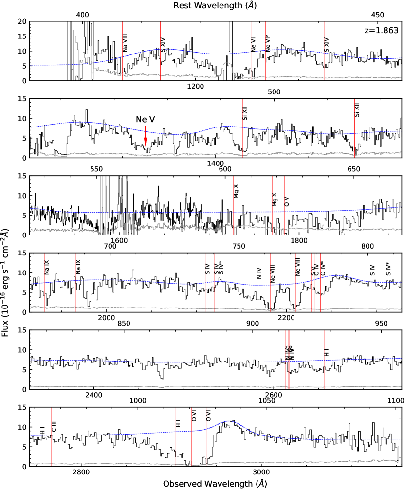
Figure 1: Co-Added STIS spectrum of Q0254-334. The absorption features of the outflow system are marked with red vertical lines, with the Ne v multiplet emphasized with a red arrow. The continuum and emission model is plotted as a blue dashed curve.

2 Observation and Data Acquisition

Q0254-334 (J2000; RA=02:56:47.84, DEC=-33:15:26.16, z=1.863) was observed with HST/STIS on 17 February, 2001 as part of the program SNAP 8681, and on 4 March, 2001 as part of the program GO 8569, with the G230L and G140L gratings respectively. After retrieving the data from the Mikulski Archive for Space Telescopes, we have co-added the two spectra, and corrected the combined spectrum for galactic reddening and extinction with $E(B-V)=0.0205$ (Schlafly & Finkbeiner, 2011), and the extinction model by Fitzpatrick (1999). The co-added and dereddened spectrum of the two observations, covering observed wavelengths 1138.6–3156.6Å, is shown in Figure 1.

We have identified a broad absorption line (BAL) outflow system at $v=-3200\text{ km s}^{-1}$, with its ionic absorption troughs marked by red vertical lines in Figure 1. Troughs exist of species such as Ne viii, Na ix, and Si xii, as well as excited state transitions such as O iv* and Ne v*. Arav et al. (2020) define a BAL in the extreme UV range as a continuous absorption feature with normalized flux $I\leq 0.9$ over a width of $\Delta v\gtrsim 1500\text{ km s}^{-1}$, at least $-3000\text{ km s}^{-1}$ blueward of the center of emission. We have verified that the outflow is a BAL outflow by confirming the width of the Si xii $\lambda 499.406$ and Ne viii $\lambda 780.324$ troughs (see Figure 2). The normalized flux was found by modeling the quasar’s continuum and emission, using a power law model for the continuum, and Gaussian profiles for the emission features. The presence of the Ne v* feature allowed us to find the value of $n_{e}$, as shown in Section 3.2.

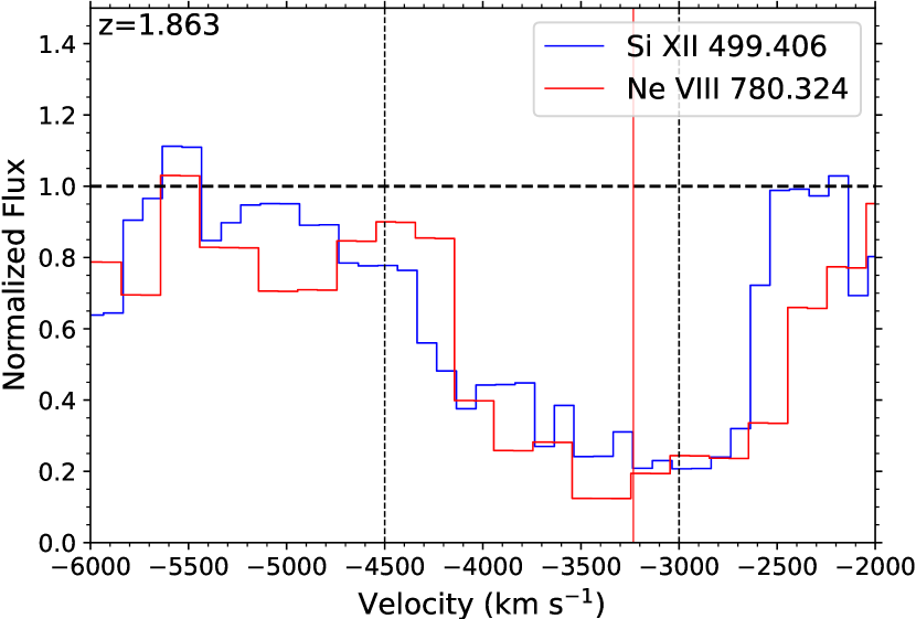
Figure 2: Normalized flux in the region of the Si xii $\lambda 499.406$ and Ne viii $\lambda 780.324$ absorption. The dashed horizontal line shows the continuum level, and the dotted vertical lines show the region between $v=-4500$ and $-3000$ km s^-1. The normalized flux for both troughs is below 0.9 in this region, showing that the absorption is a BAL outflow.

3 Analysis

3.1 Ionic Column Densities

As the ionic column densities $(N_{ion})$ of the outflow are crucial in finding the physical properties of the outflow, we used two different methods to find them based on the absorption troughs: the apparent optical depth (AOD) method in which we assume uniform and homogeneous covering (Savage & Sembach, 1991); and the partial covering (PC) method in which we include a covering factor $C<1$ (Barlow et al., 1997; Arav et al., 1999b; Arav et al., 1999a).

The AOD method allows us to find upper limits and lower limits of ionic column densities with its relative simplicity, while the PC method lets us find more accurate measurements of ions with doublet features (e.g. de Kool et al., 2002; Arav et al., 2005; Borguet et al., 2012a; Byun et al., 2022b). Section 3.1 of Byun et al. (2022c) describes these methods in further detail, as they used the same methods to analyze the outflow of the quasar J024221.87+004912.6.

For each ion, we converted the spectrum from wavelength space to velocity space, using the redshift of the quasar and the wavelengths of the ionic transition lines (see Figures 3,4). We then chose integration ranges for each ion that covered visible absorption features and minimized blending effects with other lines. For instance, the O vi doublet had heavy blending between the red and blue troughs (see Figure 3(f)). We thus chose a range where the overlap between the red and blue troughs would be minimized and computed a lower limit to the column density with the AOD method. As there were no discernible absorption troughs of Ly $\gamma$, C iii, and S iv*, we measured their AOD column density with integration range $v\approx-4000$ to $-2000$ km s^-1, and treated them as upper limits. Due to the severe blending in the multiplet of S iv $\lambda\lambda 744.904,748.393$ and S iv* $\lambda 750.221$ (see panel 4 of Figure 1), we were unable to pinpoint the column density of the resonance state S iv 0 from this trough. However, as there was no discernible absorption trough of S iv $\lambda 809.656$, we were able to find an upper limit of its column density. Similarly, the trough of O iv $\lambda 787.711$ blended with O iv* $\lambda 790.190$, and potentially with the neighboring S v $\lambda 786.468$. As such, we were unable to find the column density of the resonance state O iv 0, and could only find a lower limit of the O iv* column density. We were also limited to finding a lower limit of the Ne viii column density based on an AOD measurement due to the saturation of the doublet troughs. We determined the red trough of S xiv $\lambda 446$ to be contaminated, due to the visible blue-ward absorption compared to the blue trough $\lambda 418$ (see Figure 4 plot c). Due to this limitation, we measured the AOD column density of S xiv based on the blue trough. We determined that it was safe to treat this column density as a measurement, due to its shallower depth relative to similarly ionized troughs with comparable oscillator strengths (e.g. Si xii).

The integrated column densities are shown in Table 1. The rightmost column shows the values adopted for the photoionization solution described in Section 3.3. The errors have been propagated from the error in the flux, and a 20% error has been added in quadrature to the adopted column density errors to account for the uncertainty in the continuum level (Xu et al., 2018). Note that the column density of Ne v was based on a Gaussian fit of the troughs of its different energy states, which we further describe in Section 3.2.

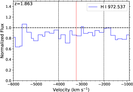
(a) H i

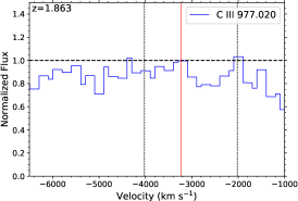
(b) C iii

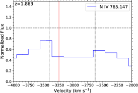
(c) N iv

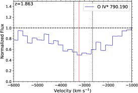
(d) O iv*

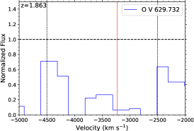
(e) O v

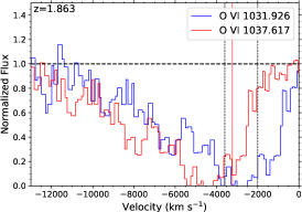
(f) O vi

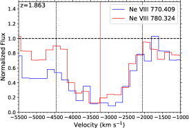
(g) Ne viii

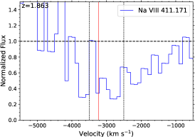
(h) Na viii

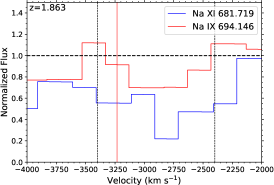
(i) Na ix

Figure 3: Absorption troughs of the Q0254-334 outflow plotted in velocity space. The velocity of the outflow at $z=1.89229$ is marked with red vertical lines. The integration range used to calculate the column densities is marked with dotted vertical lines, while the continuum level is indicated by the dashed horizontal line.

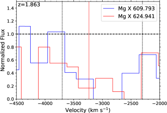
(a) Mg x

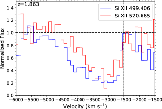
(b) Si xii

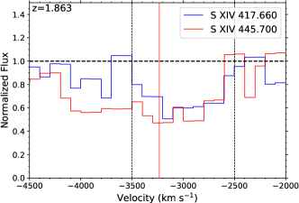
(c) S xiv

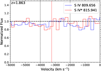
(d) S iv

Figure 4: Absorption troughs of Mg x, Si xii, S xiv, and S iv* in the outflow of Q0254-334. Format and notation are identical to those of Figure 3.

Table 1: Q0254-334 outflow column densities from STIS observations. The numbers next to the Ne v* excited states denote the energies in cm^-1. The values are in units of $10^{14}$ cm^-2.

Ion	AOD	PC	Adopted
H i	$31_{-4}^{+7}$		$<31^{+9}$
C iii	$1.3_{-0.2}^{+0.2}$		$<1.3^{+0.3}$
N iv	$5.7_{-0.4}^{+0.6}$		$>5.7_{-1.2}$
O iv*	$26.2_{-1.9}^{+2.4}$		$>26.2_{-5.6}$
O v	$52_{-5}^{+8}$		$>52_{-12}$
O vi	$123_{-5}^{+9}$		$>123_{-25}$
Ne v total	$200_{-23}^{+23}$		$200_{-46}^{+46}$
Ne v 0	$118_{-20}^{+20}$
Ne v* 411	$67_{-11}^{+11}$
Ne v* 1109	$15_{-3}^{+3}$
Ne viii	$286_{-11}^{+22}$		$>286_{-58}$
Na viii	$24_{-3.1}^{+11.9}$		$>24_{-5.7}$
Na ix	$36.8_{-6.8}^{+8.3}$	$53.6_{-7.2}^{+12.2}$	$53.6_{-12.9}^{+16.2}$
Mg x	$225_{-30}^{+45}$		$>225_{-54}$
Si xii	$410_{-24}^{+48}$		$>410_{-86}$
S iv total	$25^{+3}_{-3}$		$<25^{+6}$
S iv 0	$9.4^{+1.4}_{-1.6}$
S iv*	$16^{+2}_{-2}$
S xiv	$207_{-14}^{+19}$		$207_{-44}^{+46}$

3.2 Ne v Gaussian Fitting

As seen in Figure 5 (top panel), the Ne v multiplet of the outflow is blended into a singular trough. To remedy this, we modeled the individual energy states of Ne v by fitting Gaussian profiles for each of the expected absorption features, and running a best fit algorithm to best match the data. The free parameters used were the optical depth of the ground state Ne v trough, the width of the trough, and $\log{n_{e}}$. We assumed the AOD scenario, and adjusted the depths of the excited state troughs to match the oscillator strengths of the transition lines, as well as the abundance ratios $N(\text{Ne\,{v}}*)/N(\text{Ne\,{v}}\text{ }0)$ from the Chianti 9.0.1 atomic database (Dere et al., 1997; Dere et al., 2019). We assumed a temperature of 10,000 K in our Chianti computations.

We have found that the optical depth $\tau=0.75\pm{0.11}$, $\text{FWHM}=2440\pm{170}\text{ km s}^{-1}$ and $\log{n_{e}}=3.5\pm{0.2}\text{ }[\text{cm }^{-3}]$. Using the modeled troughs, we have calculated the column densities of each energy state of Ne v, as shown in Table 1. Since the value of $n_{e}$ is crucial in finding the distance of the outflow from the central source (as described in Section 4), we later ran a simulation with the spectral synthesis code Cloudy (version c17.00, Ferland et al., 2017) in order to verify the temperature of the outflow. With the two-phase high-ionization solution later described in Section 3.3 as our input parameters, the simulation yielded a temperature of $T\approx 32,000\text{ K}$. Calculating the electron number density with this temperature yielded $\log{n_{e}}=4.0_{-0.2}^{+0.2}$. As such, we adopted this value of $\log{n_{e}}$ for the purpose of our analysis. The total column density of Ne v based on this computation is in agreement with the value based on the $T=10,000$ K assumption.

As an alternate method of modeling the blended trough of the Ne v multiplet, we used the trough of Si xii $\lambda 499$ as a template to create a profile of two blended Gaussians (see Figure 6). We then ran a best fit algorithm to model the absorption of each energy state, leaving the width of the profile as a fixed parameter (see Figure 5 bottom panel). This resulted in an electron number density of $\log{n_{e}}=4.3\pm 0.1$ [cm^-3], which is only $\sim 0.3$ dex higher than the simple Gaussian fitting shown in Section 3.2. We report the physical properties calculated based on this value of $n_{e}$ in Table 4.

While the difference in the electron number density shifts the kinetic luminosity to lower values relative to those shown in Table 2, the kinetic luminosities remain in agreement within error. We thus focus on the results based on the Gaussian model throughout the paper. The parameters are described in further detail in Sections 4 and 5.

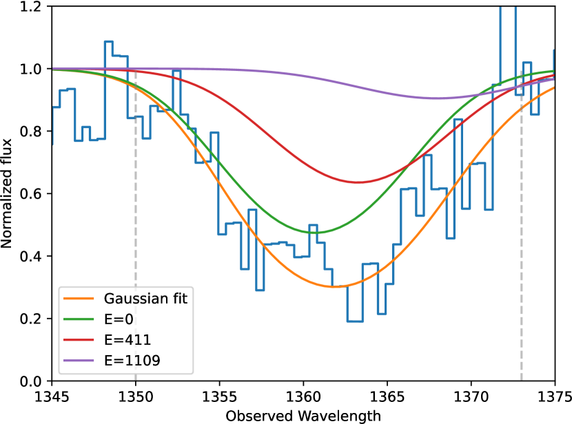
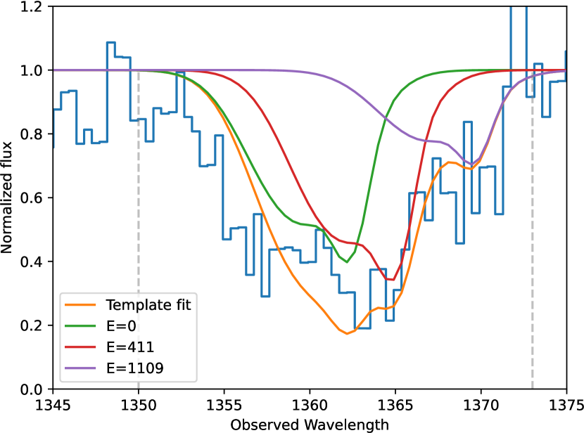
Figure 5: Modeling of the Ne v absorption troughs, created by fitting Gaussians (top) and by using Si xii as a template (bottom). The vertical dashed lines represent the range of data used for our fitting. The green curve is the modeled absorption of the resonance state of Ne v. The red curve shows combined absorption of the $E=411\text{ cm${{}^{-}1}$}$ level lines, and the purple curve shows the absorption of the $E=1109\text{ cm${}^{-1}$}$ level lines. The orange curve represents the total combined modeled absorption of the Ne v multiplet.

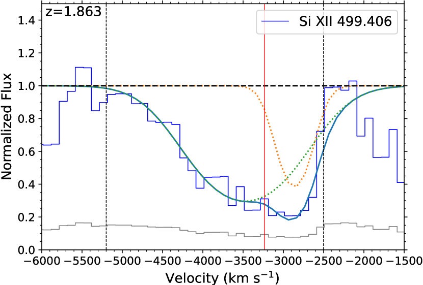
Figure 6: Fitting of a two-Gaussian profile to the absorption trough of Si xii. The dotted curves show the individual Gaussians in the profile, while the blue curve shows the blended profile of both Gaussians. The dotted vertical lines represent the range of data that was used for fitting the Gaussians.

3.3 Photoionization Solution

We used the measured ionic column densities to constrain the values of the hydrogen column density ($N_{H}$) and ionization parameter ($U_{H}$), as done in previous works (e.g Xu et al., 2019; Byun et al., 2022a, b, c; Walker et al., 2022). For this purpose, we used a grid of simulated models produced with Cloudy (Ferland et al., 2017) with a range of $N_{H}$ and $U_{H}$ values as input parameters, modeling the ionic abundances at different $N_{H}$ and $U_{H}$. We used the ionic column densities shown in Table 1 to set upper and lower limits to these parameters, as shown in Figure 8, assuming solar metallicity. We adopted a spectral energy distribution (SED) that would match the V-band flux of Q0254-334 found on NED, the UV continuum flux measured at three separate points, as well as the X-Ray fluxes observed with Chandra at energy ranges from 0.5–7 keV (see Figure 7). A single phase solution was insufficient to satisfy the constraints from the ionic column densities. To remedy this issue, we formulated a two-phase solution, in which a high- and very high-ionization phase exist co-spatially. We find that the two-phase solution satisfies more of the constraints set by the measured ionic column densities (reduced $\chi^{2}=5.7$, as opposed to $21.0$ for the one-phase solution). To cover the range of possible metallicities, we have also applied models of metallicity $Z\approx 4.68Z_{\odot}$ (Ballero et al., 2008; Miller et al., 2020b), which are shown in the lower panel of Figure 8. The results are favorable towards the super-solar metallicity solution, of which the reduced $\chi^{2}$ values are 16.0 and 0.7, for the one-phase and two-phase solutions respectively. As discussed by Arav et al. (2013), the inability for a one-phase ionization solution to reasonably fit the measurements and limits of $N_{ion}$ necessitates the adoption of a two-phase solution. The $U_{H}$ and $N_{H}$ values found using $\chi^{2}$ analysis are shown in Table 2.

We compared the $N_{H}$ and $U_{H}$ values found using the Q0254-334 SED with those found using the SED of the quasar HE0238-1904 (hereafter HE0238, Arav et al., 2013), as the latter SED has been adopted for quasar outflow analysis in several past papers (e.g., Miller et al., 2020a; Byun et al., 2022a, b, c; Walker et al., 2022). We report the $\log{N_{H}}$ and $\log{U_{H}}$ values derived from the HE0238 SED in Table 3. Comparing these values with those found in Table 2 shows that while the one-phase solutions are in agreement within error, the two-phase solutions show a discrepancy in the $\log{U_{H}}$ values that range up to $\sim 0.4$ dex.

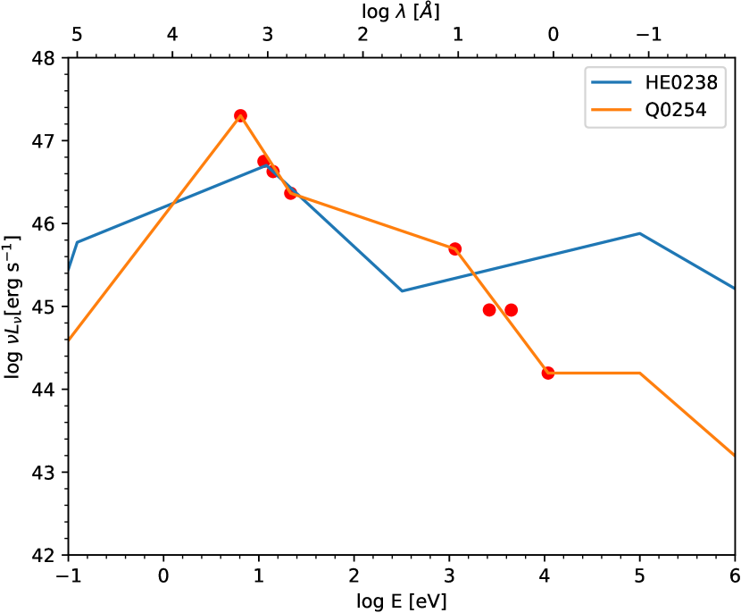
Figure 7: Comparison of SED shapes of HE0238 (Arav et al., 2013) and Q0254-334. The Q0254-334 SED was formed by using the V-band magnitude (the first red dot, Rao et al., 2006), UV continuum flux measured at three different wavelengths (rest wavelengths $\lambda=574,880,1097$ Å; second, third, and fourth red dots), and the X-ray fluxes reported by Chandra (5th–8th dots). The HE0238 SED was scaled to match the UV continuum flux for the sake of this comparison. We use the Q0254-334 SED for the analysis in this paper.

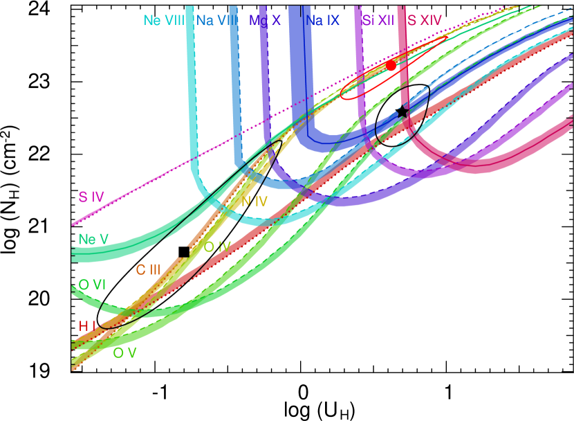
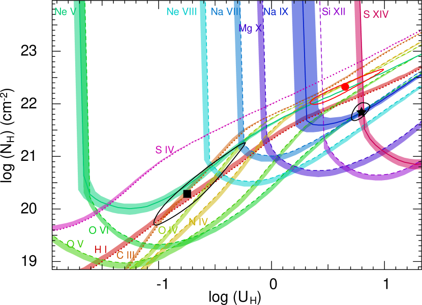
Figure 8: Plots of the Hydrogen column density ($N_{H}$) vs. ionization parameter ($U_{H}$), assuming solar (top) and supersolar (bottom) metallicities, with the Q0254-334 SED shown in Figure 7. Constraints on the parameters are based on measured column densities shown in Table 1. Measurements are shown as solid curves, while upper and lower limits are represented with dotted and dashed curves, respectively. The colored bands represent the uncertainties in the constraints. The red circle shows the one-phase solution of $N_{H}$ and $U_{H}$, while the black square and star show the high ionization and very high-ionization phase of the two-phase solution respectively. The 1-$\sigma$ uncertainties of the solutions are shown as black/red ellipses.

3.4 Black Hole Mass Calculation

Black hole masses of AGN are often found using the emission features of Mg ii (Bahk et al., 2019) or C iv (Vestergaard & Peterson, 2006; Coatman et al., 2017). However, as the STIS spectrum of Q0254-334 lacked both features, we looked to the O vi emission to compute the mass of the central black hole. We referred to the method described by Tilton & Shull (2013), measuring the O vi FWHM to find the mass.

Although Tilton & Shull (2013) specify the use of two Gaussians to fit each line of the emission doublet, we opted to fit one Gaussian per line instead, as the lower signal to noise ratio of the STIS spectrum did not warrant the more detailed modeling method. We employed a best fit algorithm adjusting the amplitude of the blue emission line, the ratio between the blue and red lines, and the FWHM of the blue line. The ratio between the blue and red line amplitudes was constrained between 1–1.5, and the widths of the two features were fixed to be equal to each other. For the resulting fit, we found a ratio of 1, normalized amplitude $A=0.24\pm 0.14$, and $\text{FWHM}=4800\pm 1000\text{ km s${}^{-1}$}$. This, along with the measured flux of $F_{\lambda}=7.7^{+1.0}_{-1.0}\times 10^{-16}\text{ erg s${}^{-1}$ cm${}^{-2}$ \AA${}^{-1}$}$ at rest wavelength $1050$Å, resulted in a black hole mass of $M_{BH}=5.0^{+5.6}_{-2.7}\times 10^{9}M_{\odot}$, and Eddington luminosity $L_{Edd}=6.4^{+7.0}_{-3.3}\times 10^{47}\text{ erg s}^{-1}$. Note that we have limited our Gaussian fit to the red wing of the emission feature, as the blue wing has been contaminated by the absorption outflow (see Fig. 9). While this contamination has contributed significantly to the uncertainty, we were unable to find alternative emission features with which to estimate the black hole mass.

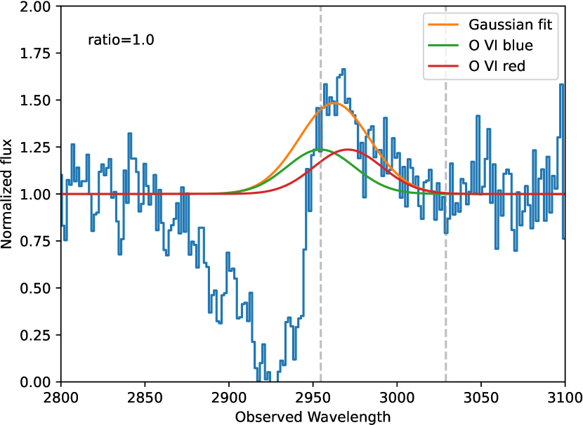
Figure 9: Gaussian fitting of the O vi emission feature. The dashed vertical lines denote the range of data used for the Gaussian fit. The green and red curves are the modeled blue and red emission features respectively, and the orange curve represents the combined modeled emission.

4 Results

With the parameters we found as described in Section 3, we could calculate the distance of the outflow from the central source, as well as the kinetic luminosity of the outflow. The distance can be found based on the definition of the ionization parameter $U_{H}$:

$$U_{H}\equiv\frac{Q_{H}}{4\uppi R^{2}n_{H}c}$$ (1)

where $Q_{H}$ is the emission rate of ionizing photons, $R$ is the outflow distance from the source, $n_{H}$ is the hydrogen number density, and $c$ is the speed of light. Solving the equation for $R$ gives us

$$R=\sqrt{\frac{Q_{H}}{4\uppi U_{H}n_{H}c}}$$ (2)

For highly ionized plasma, $n_{e}\approx 1.2n_{H}$ (Osterbrock & Ferland, 2006), and the values of $U_{H}$ and $n_{e}$ were found in Section 3.

We followed the method of other works (e.g. Miller et al., 2020a; Byun et al., 2022a, c) to find $Q_{H}$ and integrated over the SED mentioned in Subsection 3.3, limiting our range to energies over 1 Ryd. This yielded the bolometric luminosity $L_{Bol}=2.40^{+0.24}_{-0.24}\times 10^{47}\text{ erg s${}^{-1}$}$ and $Q_{H}=9.33^{+0.94}_{-0.94}\times 10^{56}\text{ s${}^{-1}$}$. The distance estimates of the outflow calculated with this value are shown in Tables 2 and 4.

Table 2: Physical Properties of the Q0254-334 Outflow. The high and very high ionization phases for the two-phase solution are assumed to be co-spatial.

Metallicity	$Z_{\odot}$			$4.68Z_{\odot}$
Solution	One-phase	Two-phase		One-phase	Two-phase
Phase		High	Very High		High	Very High
$log(N_{\text{H}})$
	$23.23^{+0.40}_{-0.47}$	$20.66^{+1.54}_{-1.06}$	$22.59^{+0.37}_{-0.48}$	$22.32^{+0.33}_{-0.33}$	$20.29^{+0.97}_{-0.60}$	$21.84^{+0.18}_{-0.16}$
$[\text{cm}^{-2}]$
$log(U_{\text{H}})$
	$0.62^{+0.39}_{-0.35}$	$-0.80^{+0.67}_{-0.60}$	$0.71^{+0.18}_{-0.19}$	$0.65^{+0.34}_{-0.31}$	$-0.75^{+0.52}_{-0.30}$	$0.80^{+0.07}_{-0.09}$
$[\text{dex}]$
$log(n_{\text{e}})$
	$4.0^{+0.2}_{-0.2}$	$4.0^{+0.2}_{-0.2}$	$2.5^{+0.7}_{-0.7}$	$4.0^{+0.2}_{-0.2}$	$4.0^{+0.2}_{-0.2}$	$2.5^{+0.6}_{-0.4}$
$[\text{cm}^{-3}]$
Distance
	$90^{+50}_{-30}$	$460^{+480}_{-250}$		$90^{+40}_{-30}$	$400^{+190}_{-180}$
$[\text{pc}]$
$\dot{M}$
	$1400^{+900}_{-700}$	$1700^{+400}_{-600}$		$170^{+90}_{-60}$	$260^{+50}_{-60}$
$[M_{\odot}\text{yr}^{-1}]$
$\dot{M}v$
	$29^{+19}_{-15}$	$34^{+7}_{-13}$		$3^{+2}_{-1}$	$5^{+1}_{-1}$
$[10^{36}\text{ ergs cm}^{-1}]$
$log({\dot{E}}_{k})$
	$45.67^{+0.30}_{-0.22}$	$45.74^{+0.20}_{-0.08}$		$44.75^{+0.19}_{-0.18}$	$44.94^{+0.09}_{-0.11}$
$[\text{erg s}^{-1}]$
${\dot{E}}_{k}/L_{Edd}$
	$0.7^{+1.3}_{-0.4}$	$0.9^{+1.2}_{-0.5}$		$0.09^{+0.12}_{-0.05}$	$0.14^{+0.16}_{-0.07}$
$[\text{\%}]$
${\dot{E}}_{k}/L_{Bol}$
	$1.9^{+2.0}_{-0.8}$	$2.3^{+1.4}_{-0.4}$		$0.2^{+0.1}_{-0.1}$	$0.4^{+0.1}_{-0.1}$
$[\text{\%}]$

Table 3: Photoionization solution for the Q0254-334 outflow assuming the HE0238 SED.

Metallicity	$Z_{\odot}$			$4.68Z_{\odot}$
Solution	One-phase	Two-phase		One-phase	Two-phase
Phase		High	Very High		High	Very High
$log(N_{\text{H}})$
	$23.08^{+0.38}_{-0.36}$	$20.80^{+0.96}_{-0.61}$	$22.57^{+0.23}_{-0.23}$	$22.31^{+0.34}_{-0.35}$	$20.66^{+1.54}_{-1.06}$	$22.59^{+0.37}_{-0.48}$
$[\text{cm}^{-2}]$
$log(U_{\text{H}})$
	$0.88^{+0.30}_{-0.23}$	$-0.40^{+0.51}_{-0.37}$	$1.01^{+0.07}_{-0.10}$	$0.89^{+0.27}_{-0.26}$	$-0.80^{+0.67}_{-0.60}$	$0.71^{+0.18}_{-0.19}$
$[\text{dex}]$

5 Discussion

5.1 Contribution of the Outflow to AGN Feedback

For an outflow to contribute to AGN feedback, its kinetic luminosity must be at least $\sim 0.5\%$ (Hopkins & Elvis, 2010) or $\sim 5\%$ (Scannapieco & Oh, 2004) of the quasar’s Eddington luminosity. Assuming an incomplete spherical shell, the mass flow rate can be calculated as follows:

$$\dot{M}\simeq 4\uppi\Omega RN_{H}\mu m_{p}v$$ (3)

followed by the kinetic luminosity:

$$\dot{E}_{k}\simeq\frac{1}{2}\dot{M}v^{2}$$ (4)

where $\Omega$ is the global covering factor, $\mu=1.4$ is the mean atomic mass per proton, $v$ is outflow velocity, and $m_{p}$ is the mass of a proton (Borguet et al., 2012a). We assumed $\Omega=0.2$, as C iv BALs are found in $\sim 20\%$ of quasars (Hewett & Foltz, 2003). Assuming solar metallicity, this calculation yielded a kinetic luminosity of $\log{\dot{E}_{k}}=45.67^{+0.30}_{-0.22}[\text{erg s${}^{-1}$}]$ for the one-phase solution, and $\log{\dot{E}_{k}}=45.74^{+0.20}_{-0.08}[\text{erg s${}^{-1}$}]$ for the two-phase solution, with the two kinetic luminosity values in agreement.

The ratio between the kinetic luminosity and Eddington luminosity yields $\dot{E}_{k}/L_{Edd}=0.7^{+1.3}_{-0.4}\%$ for the one-phase solution, and $\dot{E}_{k}/L_{Edd}=0.9^{+1.2}_{-0.5}\%$ for the two-phase solution, between the $0.5\%$ and $5\%$threshold. For the sake of completeness, we have also found the ratio between $\dot{E}_{k}$ and the bolometric luminosity $L_{Bol}$, resulting in $\dot{E}_{k}/L_{Bol}=2.3^{+1.4}_{-0.4}\%$ (see Table 2). Based on the ratio between $\dot{E}_{k}$ and $L_{Edd}$, the outflow would potentially be able to contribute to AGN feedback. It is important to note that the different assumed metallicity values have significant effects on the physical parameters of the outflow, such as a near order of magnitude difference in kinetic luminosity, leading to values that are insufficient for AGN feedback contribution (see Table 2).

5.2 The Two-Phase Outflow

As mentioned earlier in Section 3.3, the two-phase photoionization solution provides a better fit to the constraints from the measured ionic column densities. While the values of $\dot{E}_{k}$ for the one-phase and two-phase solutions agree with each other within error (see Table 2), there are significant differences to be found in the other parameters, such as distance, $N_{H}$, and $U_{H}$.

Note that the difference in $N_{H}$ between the high- and very high-ionization phases is $\sim 2$ orders of magnitude, while the difference in $U_{H}$ is $\sim 1.5$ orders of magnitude as well. Assuming the two phases are co-spatial, the volume filling factor of the high-ionization phase is as follows (Arav et al., 2013; Miller et al., 2020a):

$$f_{\mathrm{V}}=\frac{U_{H,HP}}{U_{H,VHP}}\times\frac{N_{H,HP}}{N_{H,VHP}}$$ (5)

resulting in $\log{f_{\mathrm{V}}}=-3.4^{+1.8}_{-1.3}$, which follows our expectations from the high-ionization phase’s larger $n_{e}$ and smaller $N_{H}$ values compared to those of the very high-ionization phase.

5.3 Connection to X-Ray Warm Absorbers

The two-phase solution for the outflow of Q0254-334 is comparable to the parameters measured in X-ray warm absorbers. For instance, in their analysis of the Seyfert galaxy NGC 3783, Netzer et al. (2003) found the parameters of the absorbing gas according to three different models, with the oxygen ionization parameter ranging from $\log{U_{ox}}=-2.4$ to $-0.6$. To effectively compare the $U_{H}$ of Q0254-334 to the $U_{ox}$ values of NGC 3783, we calculated the oxygen ionizing emission rate $Q_{ox}$ as defined below:

$$Q_{ox}=\int_{\nu(0.54\text{ keV})}^{\nu(10\text{ keV})}\frac{L_{\nu}}{h\nu}d\nu$$ (6)

such that the ratio $\frac{Q_{ox}}{Q_{H}}=\frac{U_{ox}}{U_{H}}$. The resulting value of the emission rate was $Q_{ox}=3.9^{+0.4}_{-0.4}\times 10^{54}\text{ s}^{-1}$, which is $2.4\pm{0.1}$ orders of magnitude smaller than $Q_{H}$. Subtracting $2.4\pm{0.1}$ from the $\log{U_{H}}$ values of the high- and very high-ionization phases leads to $\log{U_{ox}}=-3.2^{+0.5}_{-0.3}$ and $-1.6^{+0.1}_{-0.1}$ respectively. The very high-ionization phase has a $U_{ox}$ within the range of $U_{ox}$ values of the NGC 3783 absorbing gas.

Table 4: Physical Properties of the Q0254-334 Outflow, based on the Si xii template-based fitting of the Ne v absorption. The high and very high ionization phases for the two-phase solution are assumed to be co-spatial.

Metallicity	$Z_{\odot}$			$4.68Z_{\odot}$
Solution	One-phase	Two-phase		One-phase	Two-phase
Phase		High	Very High		High	Very High
$log(n_{\text{e}})$
	$4.3^{+0.1}_{-0.1}$	$4.3^{+0.1}_{-0.1}$	$2.8^{+0.7}_{-0.6}$	$4.3^{+0.1}_{-0.1}$	$4.3^{+0.1}_{-0.1}$	$2.8^{+0.5}_{-0.3}$
$[\text{cm}^{-3}]$
Distance
	$60^{+30}_{-20}$	$310^{+320}_{-170}$		$60^{+30}_{-20}$	$300^{+130}_{-130}$
$[\text{pc}]$
$\dot{M}$
	$1000^{+600}_{-500}$	$1100^{+200}_{-400}$		$100^{+60}_{-40}$	$190^{+20}_{-40}$
$[M_{\odot}\text{yr}^{-1}]$
$\dot{M}v$
	$20^{+12}_{-10}$	$23^{+4}_{-8}$		$2.4^{+1.0}_{-0.8}$	$3.9^{+0.5}_{-0.7}$
$[10^{36}\text{ ergs cm}^{-1}]$
$log({\dot{E}}_{k})$
	$45.50^{+0.30}_{-0.21}$	$45.57^{+0.19}_{-0.06}$		$44.58^{+0.18}_{-0.17}$	$44.80^{+0.09}_{-0.05}$
$[\text{erg s}^{-1}]$
${\dot{E}}_{k}/L_{Edd}$
	$0.5^{+0.9}_{-0.3}$	$0.6^{+0.8}_{-0.3}$		$0.06^{+0.08}_{-0.03}$	$0.09^{+0.11}_{-0.05}$
$[\text{\%}]$
${\dot{E}}_{k}/L_{Bol}$
	$1.3^{+1.3}_{-0.5}$	$1.6^{+0.9}_{-0.2}$		$0.16^{+0.09}_{-0.05}$	$0.26^{+0.07}_{-0.04}$
$[\text{\%}]$

5.4 Comparison to Other Extreme UV Objects

As the spectrum of Q0254-334 covers observed wavelengths as short as 400Å, we found it appropriate to compare it with other quasars observed in the extreme UV range (hereafter EUV500, Arav et al., 2020). We compiled a list of the physical parameters of 28 EUV500 quasar outflow systems analyzed in previous works (Arav et al., 2020; Xu et al., 2020a, b, c; Miller et al., 2020a, b, c), and added the parameters of Q0254-334 for comparison, with a total of 29 EUV500 outflow systems. Out of the 29 outflow systems, 24, including the outflow discussed in this paper, have measurements of kinetic luminosity and distance from the source. We compared the parameters of the Q0254-334 outflow such as $\dot{E}_{K}$, $N_{H}$, $R$, and $U_{H}$, with the other 23 outflow systems.

As seen in Figure 10, no strong correlation has been found between $\log{\dot{E}_{k}}$ and $\log{L_{Edd}}$, or between $\log{\dot{E}_{k}}$ and $\log{L_{Bol}}$. 4 of the 24 outflows ($\sim 16\%$) are above the threshold of $\dot{E}_{k}/L_{Edd}\sim 5\%$, while 8 ($\sim 33\%$) are between the $0.5\%$ and $5\%$ thresholds. With regards to $L_{Bol}$, 5 of the outflow systems ($\sim 20\%$) are above the $5\%$ threshold, while 8 ($\sim 33\%$) are between the $0.5\%$ and $5\%$ thresholds. Note that while the values of $\log{\dot{E}_{k}}$ range between 41–47, $\log{L_{Edd}}$ and $\log{L_{Bol}}$ range between 47.0–47.8 and 46.6–47.6 respectively, which is much narrower than the range of $\log{\dot{E}_{k}}$. It is also indicative of the ability of line-of-sight analysis to identify outflow systems at large ranges of kinetic luminosity, as well as velocity. Figure 11 shows the $\log{N_{H}}$ and $\log{U_{H}}$ values of the high- and very high-ionization phases of each of the outflow systems. With the exception of the very high-ionization phase of the outflow system of UM425 traveling at $-9420\text{ km s${}^{-1}$}$, the high-ionization phases tend to have values of $\log{U_{H}}<0$, while the very high-ionization phases have $\log{U_{H}}>0$. Note that the very high-ionization phase of the Q0254-334 outflow has a higher $\log{U_{H}}$ value relative to the average of the other outflows. We largely attribute this to the detection of S xiv. As can be seen in Figure 8, the very high-ionization phase solution is at the intersection between the Na ix and S xiv constraints. The $\log{U_{H}}$ value is $\sim 0.3$ dex higher than what it would have been if S xiv were not detected, and the parameters were constrained by other ions such as Si xii. It is also notable that as shown in Figure 11, the $\log{U_{H}}$ of the very high-ionization phase of the Q0254-334 outflow is higher than the average $\log{U_{H}}$ of the other outflows. We suspect that future observed outflows with S xiv would yield comparably high $U_{H}$ values.

Note that there is an apparent edge in the range of $\log{N_{H}}$ and $\log{U_{H}}$ values of the outflows. In Figure 11, we have indicated the approximate locations of the hydrogen ionization front ($N_{H}\approx 10^{23}U_{H}$), as well as the He ii ionization front ($N_{H}\approx 10^{22.2}U_{H}$). The $N_{H}/U_{H}$ ratio for the He ii ionization front was calculated based on the average $\log{N_{H}}$ value at which the He ii to He iii ratio is 1:1 in a series of Cloudy models created with a range of $-2.0<\log{U_{H}}<1.0$. We used the aforementioned SED of HE0238 for the models, as this SED was used for the analysis of the majority of the EUV500 outflows in question. Interestingly, the $\log{N_{H}}$ vs. $\log{U_{H}}$ values of all of the EUV500 outflows fall under the He ii ionization front.

We also examined the ranges of $R$ and $v$ of the outflow systems (see Figure 12). To examine the correlation between distance and velocity, we conducted a weighted least squares linear fit between $\log{R}$ and $\log{|v|}$, taking into account the asymmetry of the reported errors in $R$. We adopted the weight determination method described by Barlow (2003). The weight of each data point $w_{i}=1/V_{i}$ was determined by the value of $V_{i}$:

$$V_{i}=\sigma_{i}^{2}+(1-\frac{2}{\uppi})\alpha_{i}^{2}$$ (7)

in which $\sigma_{i}=\frac{\sigma_{i}^{+}+\sigma_{i}^{-}}{2}$ is the mean of the upper and lower errors of $\log{R}$, while $\alpha_{i}=\frac{\sigma_{i}^{+}-\sigma_{i}^{-}}{2}$.

The weighted linear fit yielded a slope of $-1.08$ and an intercept of $6.44$, suggesting a negative correlation. To determine the strength of the correlation, we calculated a modified value of the coefficient of determination $r^{2}$ that would take into account the weight of each data point. The residual sum of squares $SS_{res}$ was modified so that:

$$SS_{res}=\sum_{i}w_{i}(\log{R}_{i}-f_{i})^{2}$$ (8)

where $f_{i}$ is the value of $\log{R}$ according to the linear fit. The total sum of squares $SS_{tot}$ was adjusted so that:

$$SS_{tot}=\sum_{i}w_{i}(\log{R}_{i}-\langle\log{R}\rangle)^{2}$$ (9)

where $\langle\log{R}\rangle$ is the weighted mean of $\log{R}$. The resulting value of $r^{2}=1-\frac{SS_{res}}{SS_{tot}}$ is 0.28, suggesting a weak negative correlation between $\log{R}$ and $\log{|v|}$.

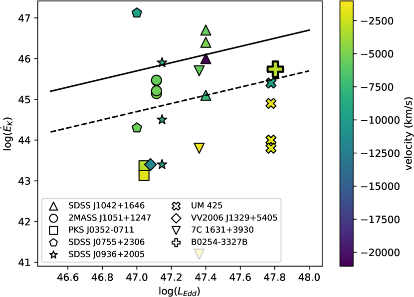
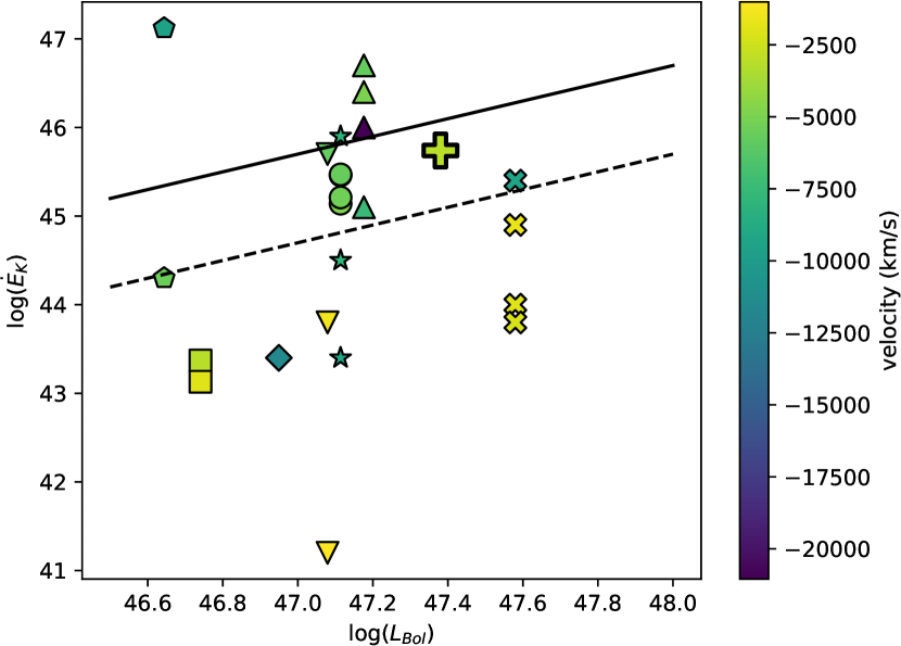
Figure 10: Distribution of $\log{\dot{E}_{k}}$ vs. $\log{L_{Edd}}$ (left) and $\log{L_{Bol}}$ (right) of EUV500 outflows. The dashed and solid lines on the left (right) indicate the $\dot{E}_{k}/L_{Edd}$ ($\dot{E}_{k}/L_{Bol}$) thresholds of $0.5\%$ and $5\%$ respectively. The plus-sign symbol denotes the outflow of Q0254-334 as reported in this paper, while the other symbols denote the parameters of other EUV outflows reported by Arav et al. (2020) and Miller et al. (2020c). The color map corresponds to the velocities of the outflow systems.

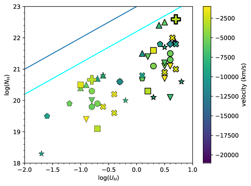
Figure 11: Distribution of $\log{N_{H}}$ vs. $\log{U_{H}}$ of EUV500 outflows. Symbols are coded as they are in Figure 10. Symbols with dotted outlines denote high-ionization phases, while symbols with solid outlines denote very high-ionization phases. The color map corresponds to the velocities of the outflow systems. The dark blue and cyan curves show the H i and He ii ionization fronts respectively.

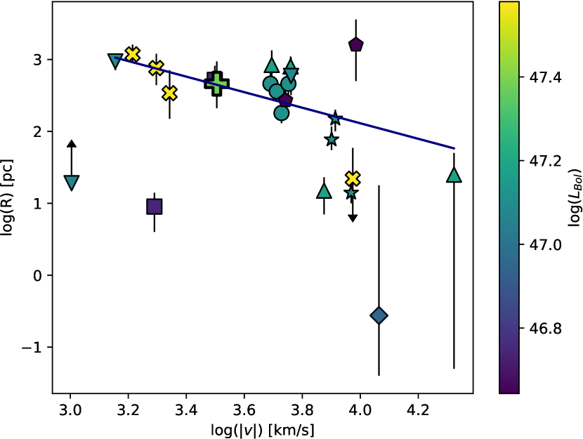
Figure 12: Distribution of $\log{R}$ vs. $\log{|v|}$ of EUV500 outflows. Symbols are coded as they are in Figure 10, with errors in $\log{R}$ indicated with error bars. The dark blue line shows the weighted least squares linear fit of $\log{R}=-1.08\times\log{|v|}+6.44$, with adjusted $r^{2}=0.28$. The color map corresponds to the $\log{L_{Bol}}$ values of the outflows.

6 Summary and Conclusion

We have identified a BAL outflow in the HST/STIS spectrum of the quasar QSO B0254-3327B, of which we have found the ionic column densities (see Table 1). Based on the column densities, we conducted photoionization analysis to find the values of hydrogen column density $N_{H}$ and ionization parameter $U_{H}$. The results of our analysis are as follows:

1. The two-phase solution. The constraints from the measured ionic column densities required a solution with two ionization phases: the high-ionization phase and the very high-ionization phase. The two-phase solution showed a significant improvement in the $\chi^{2}$ value compared to that of the one-phase solution (reduced $\chi^{2}=5.7\text{ vs. }21.0$).

2. The energetics of the outflow. We were able to determine the composition of the Ne v trough via Gaussian fitting of the blended features (see Figure 5), thanks to which we were able to narrow down the electron number density $n_{e}$. Through the use of Equations 2, 3, and 4, we were able to determine the distance, mass flow rate, and kinetic luminosity of the outflow (see Table 2). There were notable differences in the energetics parameters based on different values of assumed metallicity ($Z=Z_{\odot}$ vs $Z=4.68Z_{\odot}$, see Tables 2 and 4).

3. Potential contribution to AGN feedback. As the ratio between the kinetic luminosity and the quasar’s Eddington luminosity $\dot{E}_{k}/L_{Edd}=0.9^{+1.2}_{-0.5}\%$ assuming solar abundance, and $0.14^{+0.16}_{-0.11}$ assuming super-solar abundance, its contribution to AGN feedback is model dependent, as the theoretical thresholds for the ratio are $\sim 0.5\%$ (Hopkins & Elvis, 2010) and $\sim 5\%$ (Scannapieco & Oh, 2004).

4. Comparison to X-ray warm absorbers. We have compared the ionization parameter values of the high-ionization and very high-ionization phase to that of the X-ray warm absorber of NGC 3783 analyzed by Netzer et al. (2003). Converting $U_{H}$ to the oxygen ionization parameter $U_{ox}$ as defined by Netzer et al. (2003) showed that the $U_{ox}$ of the very high-ionization phase agreed with that of the NGC 3783 absorber within the error.

5. Comparison with other EUV500 outflows.We have also examined the physical parameters of previously studied EUV500 outflows (Arav et al., 2020; Xu et al., 2020a, b, c; Miller et al., 2020a, b, c), and determined that out of the sample of 24 outflow systems with measured kinetic luminosity, up to $\sim 50\%$ may contribute to AGN feedback, depending on the theoretical model. The trend between $\log{R}$ and $\log{|v|}$ was also analyzed via a weighted least squares linear fit, showing a weak negative correlation with coefficient of determination $r^{2}=0.28$. We have also found that the very high-ionization phase of the Q0254-334 outflow had one of the highest $U_{H}$ values of all UV absorption outflows to date.

The process of finding $\log{n_{e}}$ was limited to the examination of a blended trough of Ne v. Further observations and analyses of the quasar may reveal more excited state troughs, which could help improve the uncertainty in $\log{n_{e}}$. Studying additional EUV500 outflows will be essential in a more thorough statistical analysis of their parameters as well.

Data Availability

The data of Q0254-334 described in this paper may be obtained from the MAST archive at https://dx.doi.org/10.17909/63xd-4s51.

References

- Arav et al. (1999a) Arav N., Korista K. T., de Kool M., Junkkarinen V. T., Begelman M. C., 1999a, ApJ, 516, 27
- Arav et al. (1999b) Arav N., Becker R. H., Laurent-Muehleisen S. A., Gregg M. D., White R. L., Brotherton M. S., de Kool M., 1999b, ApJ, 524, 566
- Arav et al. (2005) Arav N., Kaastra J., Kriss G. A., Korista K. T., Gabel J., Proga D., 2005, ApJ, 620, 665
- Arav et al. (2013) Arav N., Borguet B., Chamberlain C., Edmonds D., Danforth C., 2013, MNRAS, 436, 3286
- Arav et al. (2020) Arav N., Xu X., Miller T., Kriss G. A., Plesha R., 2020, ApJS, 247, 37
- Astropy Collaboration et al. (2013) Astropy Collaboration et al., 2013, A&A, 558, A33
- Astropy Collaboration et al. (2018) Astropy Collaboration et al., 2018, AJ, 156, 123
- Bahk et al. (2019) Bahk H., Woo J.-H., Park D., 2019, ApJ, 875, 50
- Ballero et al. (2008) Ballero S. K., Matteucci F., Ciotti L., Calura F., Padovani P., 2008, A&A, 478, 335
- Barlow (2003) Barlow R., 2003, in Lyons L., Mount R., Reitmeyer R., eds, Statistical Problems in Particle Physics, Astrophysics, and Cosmology. p. 250 (arXiv:physics/0401042)
- Barlow et al. (1997) Barlow T. A., Hamann F., Sargent W. L. W., 1997, in Arav N., Shlosman I., Weymann R. J., eds, Astronomical Society of the Pacific Conference Series Vol. 128, Mass Ejection from Active Galactic Nuclei. p. 13 (arXiv:astro-ph/9705048)
- Bennett et al. (2014) Bennett C. L., Larson D., Weiland J. L., Hinshaw G., 2014, ApJ, 794, 135
- Borguet et al. (2012a) Borguet B. C. J., Edmonds D., Arav N., Dunn J., Kriss G. A., 2012a, ApJ, 751, 107
- Borguet et al. (2012b) Borguet B. C. J., Edmonds D., Arav N., Benn C., Chamberlain C., 2012b, ApJ, 758, 69
- Byun et al. (2022a) Byun D., Arav N., Walker A., 2022a, MNRAS, 516, 100
- Byun et al. (2022b) Byun D., Arav N., Hall P. B., 2022b, MNRAS, 517, 1048
- Byun et al. (2022c) Byun D., Arav N., Hall P. B., 2022c, ApJ, 927, 176
- Chamberlain et al. (2015) Chamberlain C., Arav N., Benn C., 2015, MNRAS, 450, 1085
- Choi et al. (2022) Choi H., Leighly K. M., Terndrup D. M., Dabbieri C., Gallagher S. C., Richards G. T., 2022, ApJ, 937, 74
- Coatman et al. (2017) Coatman L., Hewett P. C., Banerji M., Richards G. T., Hennawi J. F., Prochaska J. X., 2017, MNRAS, 465, 2120
- Dai et al. (2008) Dai X., Shankar F., Sivakoff G. R., 2008, ApJ, 672, 108
- Dere et al. (1997) Dere K. P., Landi E., Mason H. E., Monsignori Fossi B. C., Young P. R., 1997, A&AS, 125, 149
- Dere et al. (2019) Dere K. P., Zanna G. D., Young P. R., Landi E., Sutherland R. S., 2019, ApJS, 241, 22
- Ferland et al. (2017) Ferland G. J., et al., 2017, Rev. Mex. Astron. Astrofis., 53, 385
- Fitzpatrick (1999) Fitzpatrick E. L., 1999, PASP, 111, 63
- Hamann et al. (2001) Hamann F. W., Barlow T. A., Chaffee F. C., Foltz C. B., Weymann R. J., 2001, ApJ, 550, 142
- Harris et al. (2020) Harris C. R., et al., 2020, Nature, 585, 357
- He et al. (2022) He Z., et al., 2022, Science Advances, 8, eabk3291
- Hewett & Foltz (2003) Hewett P. C., Foltz C. B., 2003, AJ, 125, 1784
- Hopkins & Elvis (2010) Hopkins P. F., Elvis M., 2010, MNRAS, 401, 7
- Hunter (2007) Hunter J. D., 2007, Computing in Science & Engineering, 9, 90
- Knigge et al. (2008) Knigge C., Scaringi S., Goad M. R., Cottis C. E., 2008, MNRAS, 386, 1426
- Leighly et al. (2018) Leighly K. M., Terndrup D. M., Gallagher S. C., Richards G. T., Dietrich M., 2018, ApJ, 866, 7
- Miller et al. (2020a) Miller T. R., Arav N., Xu X., Kriss G. A., Plesha R. J., 2020a, ApJS, 247, 39
- Miller et al. (2020b) Miller T. R., Arav N., Xu X., Kriss G. A., Plesha R. J., 2020b, ApJS, 247, 41
- Miller et al. (2020c) Miller T. R., Arav N., Xu X., Kriss G. A., Plesha R. J., 2020c, ApJS, 249, 15
- Miller et al. (2020d) Miller T. R., Arav N., Xu X., Kriss G. A., 2020d, MNRAS, 499, 1522
- Moe et al. (2009) Moe M., Arav N., Bautista M. A., Korista K. T., 2009, ApJ, 706, 525
- Netzer et al. (2003) Netzer H., et al., 2003, ApJ, 599, 933
- Osterbrock & Ferland (2006) Osterbrock D. E., Ferland G. J., 2006, Astrophysics of gaseous nebulae and active galactic nuclei
- Rao et al. (2006) Rao S. M., Turnshek D. A., Nestor D. B., 2006, ApJ, 636, 610
- Reback et al. (2021) Reback J., et al., 2021, pandas-dev/pandas: Pandas 1.2.4, doi:10.5281/zenodo.4681666, https://doi.org/10.5281/zenodo.4681666
- Savage & Sembach (1991) Savage B. D., Sembach K. R., 1991, ApJ, 379, 245
- Scannapieco & Oh (2004) Scannapieco E., Oh S. P., 2004, ApJ, 608, 62
- Schlafly & Finkbeiner (2011) Schlafly E. F., Finkbeiner D. P., 2011, ApJ, 737, 103
- Silk & Rees (1998) Silk J., Rees M. J., 1998, A&A, 331, L1
- Tilton & Shull (2013) Tilton E. M., Shull J. M., 2013, ApJ, 774, 67
- Vayner et al. (2021) Vayner A., et al., 2021, ApJ, 919, 122
- Vestergaard & Peterson (2006) Vestergaard M., Peterson B. M., 2006, ApJ, 641, 689
- Virtanen et al. (2020) Virtanen P., et al., 2020, Nature Methods, 17, 261
- Walker et al. (2022) Walker A., Arav N., Byun D., 2022, MNRAS, 516, 3778
- Wes McKinney (2010) Wes McKinney 2010, in Stéfan van der Walt Jarrod Millman eds, Proceedings of the 9th Python in Science Conference. pp 56 – 61, doi:10.25080/Majora-92bf1922-00a
- Xu et al. (2018) Xu X., Arav N., Miller T., Benn C., 2018, ApJ, 858, 39
- Xu et al. (2019) Xu X., Arav N., Miller T., Benn C., 2019, ApJ, 876, 105
- Xu et al. (2020a) Xu X., Arav N., Miller T., Kriss G. A., Plesha R., 2020a, ApJS, 247, 38
- Xu et al. (2020b) Xu X., Arav N., Miller T., Kriss G. A., Plesha R., 2020b, ApJS, 247, 40
- Xu et al. (2020c) Xu X., Arav N., Miller T., Kriss G. A., Plesha R., 2020c, ApJS, 247, 42
- Yuan et al. (2018) Yuan F., Yoon D., Li Y.-P., Gan Z.-M., Ho L. C., Guo F., 2018, ApJ, 857, 121
- de Kool et al. (2001) de Kool M., Arav N., Becker R. H., Gregg M. D., White R. L., Laurent-Muehleisen S. A., Price T., Korista K. T., 2001, ApJ, 548, 609
- de Kool et al. (2002) de Kool M., Korista K. T., Arav N., 2002, ApJ, 580, 54