Analysis of Learning a Flow-based Generative Model from Limited Sample Complexity

Abstract

We study the problem of training a flow-based generative model, parametrized by a two-layer autoencoder, to sample from a high-dimensional Gaussian mixture. We provide a sharp end-to-end analysis of the problem. First, we provide a tight closed-form characterization of the learnt velocity field, when parametrized by a shallow denoising auto-encoder trained on a finite number $n$ of samples from the target distribution. Building on this analysis, we provide a sharp description of the corresponding generative flow, which pushes the base Gaussian density forward to an approximation of the target density. In particular, we provide closed-form formulae for the distance between the means of the generated mixture and the mean of the target mixture, which we show decays as $\Theta_{n}(\nicefrac{{1}}{{n}})$. Finally, this rate is shown to be in fact Bayes-optimal.

Flow and diffusion-based generative models have introduced a shift in paradigm for density estimation and sampling problems, leading to state-of-the art algorithms e.g. in image generation [31, 30, 33]. Instrumental in these advances was the realization that the sampling problem could be recast as a transport process from a simple –typically Gaussian– base distribution to the target density. Furthermore, the velocity field governing the flow can be characterized as the minimizer of a quadratic loss function, which can be estimated from data by (a) approximating the loss by its empirical estimate using available training data and (b) parametrizing the velocity field using a denoiser neural network. These ideas have been fruitfully implemented as part of a number of frameworks, including score-based diffusion models [35, 36, 18, 16], and stochastic interpolation [2, 1, 23, 24].

The practical success of such models however poses an intriguing theoretical puzzle: a generative model trained on the empirical loss should not, in principle, be able to differentiate between the true target density and the discrete distribution supported on the training samples. It would therefore learn a velocity field associated to the latter, and hence only allow to generate samples from the training data. In practical cases however, such a memorization is not observed, suggesting the presence of an in-built implicit regularization induced by the network parametrization.

These interrogations have yet to find a definite theoretical answer. A line of recent analytical works [3, 9, 6, 8, 10, 39, 20, 21, 22, 13, 12, 29, 5] has mainly focused on the study of the transport problem, and provides rigorous convergence guarantees, taking as a starting point the assumption of an $L^{2}-$accurate estimate of the velocity or score. They hence bypass the investigation of the learning problem –and in particular the question of ascertaining the sample complexity needed to obtain such an accurate estimate. More importantly, the study of the effect of learning from a limited sample complexity (and thus e.g. of possible network overfitting and memorization) on the generated density, is furthermore left unaddressed. On the other hand, very recent works [11, 34] have characterized the learning of Denoising Auto-Encoders (DAEs) [38, 37] in high dimensions on Gaussian mixture densities. Neither work however studies the consequences on the generative process. Bridging that gap, recent works have offered a joint analysis of the learning and generative processes. [27, 7, 40] derive rigorous bounds at finite sample complexity, under the assumption of data with a low-dimensional structure. Closer to our manuscript, a concurrent work [25] bounds the Kullback-Leibler distance between the generated and target densities, when parametrizing the flow using a ResNet, for high-dimensional graphical models. On the other hand, these bounds do not go to zero as the sample complexity increases, and are a priori not tight.

The present manuscript aims at complementing and furthering this last body of works, by providing a tight end-to-end analysis of a flow-based generative model – starting from the study of the high-dimensional learning problem with a finite number of samples, and subsequently elucidating the implications thereof on the generative process.

Main contributions

We study the problem of estimating and sampling a Gaussian mixture using a flow-based generative model, in the framework of stochastic interpolation [2, 1, 23, 24]. We consider the case where a non-linear two-layer DAE with one hidden unit is used to parametrize the velocity field of the associated flow, and is trained with a finite training set. In the high-dimensional limit,

• We provide a sharp asymptotic closed-form characterization of the learnt velocity field, as a function of the target Gaussian mixture parameters, the stochastic interpolation schedule, and the number of training samples $n$.

• We characterize the associated flow by providing a tight characterization of a small number of summary statistics, tracking the dynamics of a sample from the Gaussian base distribution as it is transported by the learnt velocity field.

• We show that even with a finite number of training samples, the learnt generative model allows to sample from a mixture whose mean asymptotically approaches the mean of the target mixture as $\Theta_{n}(\nicefrac{{1}}{{n}})$ in squared distance, with this rate being tight.

• Finally, we show that this rate is in fact Bayes-optimal.

The code used in the present manuscript is provided in this repository.

Related works

Diffusion and flow-based generative models

Score-based diffusion models [35, 36, 18, 16] build on the idea that any density can be mapped to a Gaussian density by degrading samples through an Ornstein-Uhlenbeck process. Sampling from the original density can then be carried out by time-reversing the corresponding stochastic transport, provided the score is known – or estimated. These ideas were subsequently refined in [2, 1, 23, 24], which provide a flexible framework to bridge between two arbitrary densities in finite time.

Convergence bounds

In the wake of the practical successes of flow and diffusion-based generative models, significant theoretical effort has been devoted to studying the convergence of such methods, by bounding appropriate distances between the generated and the target densities. A common assumption of [3, 9, 6, 8, 10, 39, 20, 21, 22, 13, 12, 29, 5] is the availability of a good estimate for the score, i.e. an estimate whose average (population) squared distance with the true score is bounded by a small constant $\epsilon$. Under this assumption, [9, 20] obtain rigorous control on the Wasserstein and total variation distances with very mild assumptions on the target density. [15] explore the connections between algorithmic hardness of the score/flow approximation and the hardness of sampling in a number of graphical models.

Asymptotics for DAE learning

The backbone of flow and diffusion-based generative models is the parametrization of the score or velocity by a denoiser-type network, whose most standard realization is arguably the DAE [38, 37]. Very recent works have provided a detailed analysis of its learning on denoising tasks, for data sampled from Gaussian mixtures. [11] sharply characterize how a DAE can learn the mixture parameters with $n=\Theta_{d}(d)$ training samples when the cluster separation is $\Theta_{d}(1)$. Closer to our work, for arbitrary cluster separation, [34] rigorously show that a DAE trained with gradient descent on the denoising diffusion probabilistic model loss [16] can recover the cluster means with a polynomial number of samples. While these works complement the aforediscussed convergence studies in that they analyze the effect of a finite number of samples, neither explores the flow associated to the learnt score.

Network-parametrized models

Tying together these two body of works, a very recent line of research has addressed the problem of bounding, at finite sample complexity, appropriate distances between the generated and target densities, assuming a network-based parametrization. [27] provide such bounds when parametrizing the score using a class of ReLU networks. These bounds however suffer from the curse of dimensionality. [27, 40, 7] surmount this hurdle by assuming a target density with low-dimensional structure. On a heuristic level, [4] estimate the order of magnitude of the sample complexity needed to sample from a high-dimensional Curie-Weiss model. Finally, a work concurrent to ours [25] derives rigorous bounds for a number of high-dimensional graphical models. On the other hand, these bounds are a priori not tight, and do not go to zero as the sample complexity becomes large. The present manuscript aims at furthering this line of work, and provides a sharp analysis of a high-dimensional flow-based generative model.

I Setting

We start by giving a concise overview of the problem of sampling from a target density $\rho_{1}$ over $\mathbb{R}^{d}$ in the framework of stochastic interpolation [2, 1].

Recasting sampling as an optimization problem

Samples from $\rho_{1}$ can be generated by drawing a sample from an easy-to-sample base density $\rho_{0}$ –henceforth taken to be a standard Gaussian density $\rho_{0}=\mathcal{N}(0,\mathbb{I}_{d}$)–, and evolving it according to the flow described by the ordinary differential equation (ODE)

$$\frac{d}{dt}\bm{X}_{t}=\bm{b}(\bm{X}_{t},t),$$ (1)

for $t\in[0,1]$. Specifically, as shown in [1], if $\bm{X}_{t=0}\sim\rho_{0}$, then the final sample $\bm{X}_{t=1}$ has probability density $\rho_{1}$, if the velocity field $\bm{b}(\bm{x},t)$ governing the flow (1) is given by

$$\bm{b}(\bm{x},t)=\mathbb{E}[\dot{\alpha}(t)\bm{x}_{0}+\dot{\beta}(t)\bm{x}_{1}|\bm{x}_{t}=\bm{x}],$$ (2)

where we denoted $\bm{x}_{t}\equiv\alpha(t)\bm{x}_{0}+\beta(t)\bm{x}_{1}$ and the conditional expectation bears over $\bm{x}_{1}\sim\rho_{1}$, $\bm{x}_{0}\sim\rho_{0}$, with $\bm{x}_{0}\perp\bm{x}_{1}$. The result holds for any fixed choice of schedule functions $\alpha,\beta\in\mathcal{C}^{2}([0,1])$ satisfying $\alpha(0)=\beta(1)=1,\alpha(1)=\beta(0)=0$, and $\alpha(t)^{2}+\beta(t)^{2}>0$ for all $t\in[0,1]$.

In addition to the velocity field $\bm{b}(\bm{x},t)$, it is convenient to consider the field $\bm{f}(\bm{x},t)$, related to $\bm{b}(\bm{x},t)$ by the simple relation

$$\bm{b}(\bm{x},t)=\left(\dot{\beta}(t)-\frac{\dot{\alpha}(t)}{\alpha(t)}\beta(t)\right)\bm{f}(\bm{x},t)+\frac{\dot{\alpha}(t)}{\alpha(t)}\bm{x}.$$ (3)

Note that $\bm{f}(\bm{x},t)$ can be alternatively expressed as $\mathbb{E}[\bm{x}_{1}|\bm{x}_{t}=\bm{x}]$, and thus admits a natural interpretation as a denoising function, tasked with recovering the target value $\bm{x}_{1}$ from the interpolated (noisy) sample $\bm{x}_{t}$. The denoiser $\bm{f}(\bm{x},t)$ can furthermore characterized as the minimizer of the objective

$$\mathcal{R}[\bm{f}] =\int\limits_{0}^{1}\mathbb{E}\left\lVert\bm{f}(\bm{x}_{t},t)-\bm{x}_{1}\right\lVert^{2}dt.$$ (4)

The loss (4) is a simple sequence of quadractic denoising objectives.

Learning the velocity from data

There are several technical hurdles in carrying out the minimization (4). First, since the analytical form of $\rho_{1}$ is generically unknown, the population risk has to be approximated by its empirical version, provided a dataset $\mathcal{D}=\{\bm{x}^{\mu}_{1},\bm{x}_{0}^{\mu}\}_{\mu=1}^{n}$ of $n$ training samples $\bm{x}^{\mu}_{1}$ ($\bm{x}^{\mu}_{0}$) independently drawn from $\rho_{1}$ ($\rho_{0}$) is available. Second, the minimization in (4) bears over a time-dependent vector field $\bm{f}$. To make the optimization tractable, the latter can be parametrized at each time step $t$ by a separate neural network $\bm{f}_{\theta_{t}}(\cdot)$ with trainable parameters $\theta_{t}$. Under those approximations, the population risk (4) thus becomes

$$\hat{\mathcal{R}}(\{\theta_{t}\}_{t\in[0,1]}) =\int\limits_{0}^{1}\sum\limits_{\mu=1}^{n}\left\lVert\bm{f}_{\theta_{t}}(\bm{x}_{t}^{\mu})-\bm{x}_{1}^{\mu}\right\lVert^{2}dt.$$ (5)

Remark that in practice, the time $t$ can enter as an input of the neural network, and only one network then needs to be trained. In the present manuscript however, for technical reasons, we instead consider the case where a separate network is trained for each time step $t$. Besides, note that since the base density $\rho_{0}$ is a priori easy to sample from, one could in theory augment the dataset $\mathcal{D}$ with several samples from $\rho_{0}$ for each available $\bm{x}_{1}^{\mu}$. For conciseness, we do not examine such an augmentation technique in the present manuscript, and leave a precise investigation thereof to future work. Denoting by $\{\hat{\theta}_{t}\}_{t\in[0,1]}$ the minimizer of (5), the learnt velocity field $\hat{\bm{b}}$ is related to the trained denoiser $\bm{f}_{\hat{\theta}_{t}}$ by (4) as

$$\hat{\bm{b}}(\bm{x},t)=\left(\dot{\beta}(t)-\frac{\dot{\alpha}(t)}{\alpha(t)}\beta(t)\right)\bm{f}_{\hat{\theta}_{t}}(\bm{x})+\frac{\dot{\alpha}(t)}{\alpha(t)}\bm{x}.$$ (6)

The sampling can finally be carried out by using $\hat{\bm{b}}$ as a proxy for the unknown $\bm{b}$ in (1):

$$\frac{d}{dt}\bm{X}_{t}=\hat{\bm{b}}(\bm{X}_{t},t)$$ (7)

Note that the solution $\bm{X}_{1}$ at time $t=1$ of the ODE (7) has a law $\hat{\rho}_{1}\neq\rho_{1}$ due to the two approximations in going from the population function-space objective (4) to the empirical parametric proxy (5). The present manuscript presents a sharp analysis of the learning problem (5) and the resulting flow (7) for a solvable model, which we detail below.

Data model

We consider the case of a target density $\rho_{1}$ given by a binary isotropic and homoscedastic Gaussian mixture

$$\rho_{1}=\frac{1}{2}\mathcal{N}(\bm{\mu},\sigma^{2}\mathbb{I}_{d})+\frac{1}{2}\mathcal{N}(-\bm{\mu},\sigma^{2}\mathbb{I}_{d}).$$ (8)

Each cluster is thus centered around its mean $\pm\bm{\mu}$ and has variance $\sigma^{2}$. For definiteness, we consider here a balanced mixture, where the two clusters have equal relative probabilities, and defer the discussion of the imbalanced case to Appendix D. Note that a sample $\bm{x}_{1}^{\mu}$ can then be decomposed as $\bm{x}_{1}^{\mu}=s^{\mu}\bm{\mu}+\bm{z}^{\mu}$, with $s^{\mu}\sim\mathcal{U}(\{-1,+1\})$ and $\bm{z}^{\mu}\sim\mathcal{N}(0,\sigma^{2}\mathbb{I}_{d})$. Finally, note that the closed-form expression for the exact velocity field $\bm{b}$ (1) associated to the density $\rho_{1}$ is actually known (see e.g. [14, 1]). This manuscript explores the question whether a neural network can learn a good approximate $\hat{\bm{b}}$ thereof without any knowledge of the density $\rho_{1}$, and only from a finite number of samples drawn therefrom.

Network architecture

We consider the case where the denoising function $\bm{f}$ (4) is parametrized with a two-layer non-linear DAE with one hidden neuron, and –taking inspiration from modern practical architectures such as U-nets [32]– a trainable skip connection:

$$\bm{f}_{\bm{w}_{t},c_{t}}(\bm{x})=c_{t}\times\bm{x}+\bm{w}_{t}\times\varphi(\bm{w}_{t}^{\top}\bm{x}),$$ (9)

where $\varphi$ is assumed to tend to $1$ (resp. $-1$) as its argument tends to $+\infty$ (resp $-\infty$). Sign, tanh and erf are simple examples of such an activation function. The trainable parameters are therefore $c_{t}\in\mathbb{R},\bm{w}_{t}\in\mathbb{R}^{d}$. Note that (9) is a special case of the architecture studied in [11], and differs from the very similar network considered in [34] in its slightly more general activation ([34] address the case $\varphi=\tanh$), and in its trainable –rather than fixed– skip connection. Since we consider the case where a separate network is trained at every time step, the empirical risk (5) decouples over the time index $t$. The parameters $\bm{w}_{t},c_{t}$ of the DAE (9) should therefore minimize

$$\hat{\mathcal{R}}_{t}(\bm{w}_{t},c_{t})=\sum\limits_{\mu=1}^{n}\lVert\bm{f}_{c_{t},\bm{w}_{t}}(\bm{x}_{t}^{\mu})-\bm{x}_{1}^{\mu}\lVert^{2}+\frac{\lambda}{2}\lVert\bm{w}_{t}\lVert^{2},$$ (10)

where for generality we also allowed for the presence of a $\ell_{2}$ regularization of strength $\lambda$. We remind that $\bm{x}_{t}^{\mu}=\alpha(t)\bm{x}_{0}^{\mu}+\beta(t)\bm{x}_{1}^{\mu}$, with $\{\bm{x}_{1}^{\mu}\}_{\mu=1}^{n}$ (resp. $\{\bm{x}_{0}^{\mu}\}_{\mu=1}^{n}$) $n$ training samples independently drawn from the target density $\rho_{1}$ (8) (resp. the base density $\rho_{0}=\mathcal{N}(0,\mathbb{I}_{d})$), collected in the training set $\mathcal{D}$.

Asymptotic limit

We consider in this manuscript the asymptotic limit $d\to\infty$, with $n,\nicefrac{{\lVert\bm{\mu}\lVert^{2}}}{{d}},\sigma=\Theta_{d}(1)$. For definiteness, in the following, we set $\nicefrac{{\lVert\bm{\mu}\lVert^{2}}}{{d}}=1$. Note that [11] consider the different limit $\lVert\bm{\mu}\lVert=\Theta_{d}(1)$. [34] on the other hand address a larger range of asymptotic limits, including the present one, but does not provide tight characterizations, nor an analysis of the generative process.

II Learning

In this section, we first provide sharp closed-form characterizations of the minimizers $\hat{c}_{t},\hat{\bm{w}}_{t}$ of the objective $\hat{\mathcal{R}}_{t}$ (10). The next section discusses how these formulae can be leveraged to access a tight characterization of the associated flow.

Result II.1.

(Sharp characterization of minimizers of (10)) For any given activation $\varphi$ satisfying $\varphi(x)\xrightarrow[]{x\to\pm\infty}\pm 1$ and any $t\in[0,1]$, in the limit $d\to\infty$, $n,\nicefrac{{\lVert\bm{\mu}\lVert^{2}}}{{d}},\sigma=\Theta_{d}(1)$, the skip connection strength $\hat{c}_{t}$ minimizing (10) is given by

$$\hat{c}_{t}=\frac{\beta(t)(\lambda(1+\sigma^{2})+(n-1)\sigma^{2})}{\alpha(t)^{2}(\lambda+n-1)+\beta(t)^{2}(\lambda(1+\sigma^{2})+(n-1)\sigma^{2})}.$$ (11)

Furthermore, the learnt weight vector $\hat{\bm{w}}_{t}$ is asymptotically contained in $\mathrm{span}(\bm{\mu},\bm{\xi},\bm{\eta})$ (in the sense that its projection on the orthogonal space $\mathrm{span}(\bm{\mu},\bm{\xi},\bm{\eta})^{\perp}$ has asymptotically vanishing norm), where $\bm{\mu}$ is the cluster mean of $\rho_{1}$ (8) and

$$\bm{\xi}\equiv\sum\limits_{\mu=1}^{n}s^{\mu}\bm{x}^{\mu}_{0}, \bm{\eta}\equiv\sum\limits_{\mu=1}^{n}s^{\mu}(\bm{x}^{\mu}_{1}-s^{\mu}\bm{\mu}).$$ (12)

We remind that $s^{\mu}=\pm 1$ was defined below (8) and indicates the cluster the $\mu-$th sample $\bm{x}_{1}^{\mu}$ belongs to. The components of $\hat{\bm{w}}_{t}$ along each of these three vectors is described by the summary statistics

$$m_{t}=\frac{\bm{\mu}^{\top}\hat{\bm{w}}_{t}}{d}, q^{\xi}_{t}=\frac{\hat{\bm{w}}_{t}^{\top}\bm{\xi}}{nd}, q^{\eta}_{t}=\frac{\hat{\bm{w}}_{t}^{\top}\bm{\eta}}{nd\sigma^{2}},$$ (13)

which concentrate as $d\to\infty$ to the quantities characterized by the closed-form formulae

$$\begin{cases}m_{t}=\frac{n}{\lambda+n}\frac{\alpha(t)^{2}(\lambda+n-1)}{\alpha(t)^{2}(\lambda+n-1)+\beta(t)^{2}(\lambda(1+\sigma^{2})+(n-1)\sigma^{2})}\\ q^{\xi}_{t}=\frac{-\alpha(t)}{\lambda+n}\frac{\beta(t)(\lambda(1+\sigma^{2})+(n-1)\sigma^{2})}{\alpha(t)^{2}(\lambda+n-1)+\beta(t)^{2}(\lambda(1+\sigma^{2})+(n-1)\sigma^{2})}\\ q^{\eta}_{t}=\frac{1}{\lambda+n}\frac{\alpha(t)^{2}(\lambda+n-1)}{\alpha(t)^{2}(\lambda+n-1)+\beta(t)^{2}(\lambda(1+\sigma^{2})+(n-1)\sigma^{2})}\end{cases}.$$ (14)

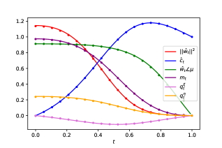
Figure 1: $n=4,\sigma=0.9,\lambda=0.1,\alpha(t)=1-t,\beta(t)=t,\varphi=\tanh.$ Solid lines: theoretical predictions of Result II.1: squared norm of the DAE weight vector $\lVert\hat{\bm{w}}_{t}\lVert^{2}$ (red), skip connection strength $\hat{c}_{t}$ (blue) cosine similarity between the weight vector $\hat{\bm{w}}_{t}$ and the target cluster mean $\bm{\mu}$, $\hat{\bm{w}}_{t}\angle\bm{\mu}\equiv\hat{\bm{w}}_{t}^{\top}\bm{\mu}/\lVert\bm{\mu}\lVert\lVert\hat{\bm{w}}_{t}\lVert$ (green), components $m_{t},q^{\xi}_{t},q^{\eta}_{t}$ of $\hat{\bm{w}}_{t}$ along the vectors $\bm{\mu},\bm{\xi},\bm{\eta}$ (purple, pink, orange). Dots: numerical simulations in dimension $d=5\times 10^{4}$, corresponding to training the DAE (9) on the risk (10) using the Pytorch implementation of full-batch Adam, with learning rate $0.0001$ over $4\times 10^{4}$ epochs and weight decay $\lambda=0.1$. The experimental points correspond to a single instance of the model.

The derivation of Result II.1 is detailed in Appendix A, and involves a heuristic partition function computation, borrowing ideas from statistical physics. The theoretical predictions for the skip connection strength $\hat{c}_{t}$ and the component $m_{t},q^{\xi}_{t},q^{\eta}_{t}$ of the weight vector $\hat{\bm{w}}_{t}$ are plotted as solid lines in Fig. 1, and display good agreement with numerical simulations, corresponding to training the DAE (9) on the risk (10) using the Pytorch [28] implementation of the Adam optimizer [19].

A notable consequence of (13) is that the weight vector $\hat{\bm{w}}_{t}$ is contained at all times $t$ in the rank$-3$ subspace spanned by the target cluster mean $\bm{\mu}$ and the vectors $\bm{\xi}$, $\bm{\eta}$ (12). $\bm{\xi},\bm{\eta}$ respectively subsume the aggregated effect of the base vectors $\{\bm{x}_{0}^{\mu}\}_{\mu=1}^{n}$ used in the train set, and of the random part $\{\bm{x}_{1}^{\mu}-s^{\mu}\bm{\mu}\}_{\mu=1}^{n}$ of the training samples $\bm{x}_{1}^{\mu}$. Rather remarkably, the training samples thus only enter in the characterization of $\hat{\bm{w}}_{t}$ through the form of simple sums (12). Since the vectors $\bm{\xi},\bm{\eta}$ represent quantities associated to the training samples, the fact that the learnt vector $\hat{\bm{w}}_{t}$ has non-zero components along $\bm{\xi},\bm{\eta}$ hence signals a form of overfitting and memorization. Interestingly, Fig. 1 shows that the extent of this overfitting is non-monotonic in time, as $|q^{\xi}_{t}|$ first increases then decreases. Finally, note that this effect is as expected mitigated as the number of training samples $n$ increases. From (14), for large $n$, $m_{t}=\Theta_{n}(1)$ while the components $q^{\xi}_{t},q^{\eta}_{t}$ along the training quantities $\bm{\xi},\bm{\eta}$ are suppressed as $\Theta_{n}(\nicefrac{{1}}{{n}})$. These scalings are further elaborated upon in Remark B.3 in Appendix B. Finally, Result II.1 and equation (6) can be straightforwardly combined to yield a sharp characterization of the learnt estimate $\hat{\bm{b}}$ of the velocity field $\bm{b}$ (1). This characterization can be in turn leveraged to build a tight description of the generative flow (7). This is the object of the following section.

III generative process

While Corollary II.1, together with the definition (6), provides a concise characterization of the velocity field $\hat{\bm{b}}$, the sampling problem (7) remains formulated as a high-dimensional, and therefore hard to analyze, transport process. The following result shows that the dynamics of a sample $\bm{X}_{t}$ following the differential equation (7) can nevertheless be succinctly tracked using a finite number of scalar summary statistics.

Result III.1.

(Summary statistics) Le $\bm{X}_{t}$ be a solution of the ordinary differential equation (7) with initial condition $\bm{X}_{0}$. For a given $t$, the projection of $\bm{X}_{t}$ on $\mathrm{span}(\bm{\mu},\bm{\xi},\bm{\eta})$ is characterized by the summary statistics

$$M_{t}\equiv\frac{\bm{X}_{t}^{\top}\bm{\mu}}{d}, Q^{\xi}_{t}\equiv\frac{\bm{X}_{t}^{\top}\bm{\xi}}{nd}, Q^{\eta}_{t}\equiv\frac{\bm{X}_{t}^{\top}\bm{\eta}}{nd\sigma^{2}}.$$ (15)

With probability asymptotically $\nicefrac{{1}}{{2}}$ the summary statistics $M_{t},Q^{\xi}_{t},Q^{\eta}_{t}$ (15) concentrate for all $t$ to the solution of the ordinary differential equations

$$\begin{cases}\frac{d}{dt}M_{t}=\left(\dot{\beta}(t)\hat{c}_{t}+\frac{\dot{\alpha}(t)}{\alpha(t)}(1-\hat{c}_{t}\beta(t))\right)M_{t}+\left(\dot{\beta}(t)-\frac{\dot{\alpha}(t)}{\alpha(t)}\beta(t)\right)m_{t}\\ \frac{d}{dt}Q^{\xi}_{t}=\left(\dot{\beta}(t)\hat{c}_{t}+\frac{\dot{\alpha}(t)}{\alpha(t)}(1-\hat{c}_{t}\beta(t))\right)Q^{\xi}_{t}+\left(\dot{\beta}(t)-\frac{\dot{\alpha}(t)}{\alpha(t)}\beta(t)\right)q^{\xi}_{t}\\ \frac{d}{dt}Q^{\eta}_{t}=\left(\dot{\beta}(t)\hat{c}_{t}+\frac{\dot{\alpha}(t)}{\alpha(t)}(1-\hat{c}_{t}\beta(t))\right)Q^{\eta}_{t}+\left(\dot{\beta}(t)-\frac{\dot{\alpha}(t)}{\alpha(t)}\beta(t)\right)q^{\eta}_{t}\end{cases},$$ (16)

with initial condition $M_{0}=Q^{\xi}_{0}=Q^{\eta}_{0}=0$, and with probability asymptotically $\nicefrac{{1}}{{2}}$ they concentrate to minus the solution of (16). Furthermore, the orthogonal component $\bm{X}_{t}^{\perp}\in\mathrm{span}(\bm{\mu},\bm{\xi},\bm{\eta})^{\perp}$ obeys the simple linear differential equation

$$\frac{d}{dt}\bm{X}_{t}^{\perp}=\left(\dot{\beta}(t)\hat{c}_{t}+\frac{\dot{\alpha}(t)}{\alpha(t)}(1-\hat{c}_{t}\beta(t))\right)\bm{X}_{t}^{\perp}.$$ (17)

Finally, the statistic $Q_{t}\equiv\nicefrac{{\lVert\bm{X}_{t}\lVert^{2}}}{{d}}$ is given with high probability by

$$Q_{t}=M_{t}^{2}+n(Q_{t}^{\xi})^{2}+n\sigma^{2}(Q_{t}^{\eta})^{2}+e^{2\int\limits_{0}^{t}\left(\dot{\beta}(t)+\frac{\dot{\alpha}(t)}{\alpha(t)}(1-\hat{c}_{t}\beta(t))\right)dt}.$$ (18)

A heuristic derivation of Result III.1 is provided in Appendix B. Taking a closer look at (16), it might seem at first from equations (16) that there is a singularity for $t=1$ since $\alpha(1)=0$ in the denominator. Remark however that both $1-\beta(t)\hat{c}_{t}$ (11) and $m_{t}$ (14) are actually proportional to $\alpha(t)^{2}$, and therefore (16) is in fact also well defined for $t=1$. In practice, the numerical implementation of a generative flow like (7) often involves a discretization thereof, given a discretization scheme $\{t_{k}\}_{k=0}^{N}$ of $[0,1]$, where $t_{0}=0$ and $t_{N}=1$:

$$\bm{X}_{t_{k+1}}=\bm{X}_{t_{k}}+\hat{\bm{b}}(\bm{X}_{t_{k}},t_{k})(t_{k+1}-t_{k}).$$ (19)

The evolution of the summary statistics introduced in Result III.1 can be rephrased in more actionable form to track the discretized flow (19).

Remark III.2.

(Summary statistics for the discrete flow) Let $\{\bm{X}_{t_{k}}\}_{k=0}^{N}$ be a solution of the discretized learnt flow (7), for an arbitrary discretization scheme $\{t_{k}\}_{k=0}^{N}$ of $[0,1]$, where $t_{0}=0$ and $t_{N}=1$, with initial condition $\bm{X}_{t_{0}}\sim\rho_{0}$. The summary statistics introduced in Result III.1 are then equal to the solutions of the recursions

$$\begin{cases}M_{t_{k+1}}=M_{t_{k}}+\delta t_{k}\left(\dot{\beta}(t_{k})\hat{c}_{t_{k}}+\frac{\dot{\alpha}(t_{k})}{\alpha(t_{k})}(1-\hat{c}_{t_{k}}\beta(t_{k}))\right)M_{t_{k}}+\delta t_{k}\left(\dot{\beta}(t_{k})-\frac{\dot{\alpha}(t_{k})}{\alpha(t_{k})}\beta(t_{k})\right)m_{t_{k}}\\ Q^{\xi}_{t_{k+1}}=Q^{\xi}_{t_{k}}+\delta t_{k}\left(\dot{\beta}(t_{k})\hat{c}_{t_{k}}+\frac{\dot{\alpha}(t_{k})}{\alpha(t_{k})}(1-\hat{c}_{t_{k}}\beta(t_{k}))\right)Q^{\xi}_{t_{k}}+\delta t_{k}\left(\dot{\beta}(t_{k})-\frac{\dot{\alpha}(t_{k})}{\alpha(t_{k})}\beta(t_{k})\right)q^{\xi}_{t_{k}}\\ Q^{\eta}_{t_{k+1}}=Q^{\eta}_{t_{k}}+\delta t_{k}\left(\dot{\beta}(t_{k})\hat{c}_{t_{k}}+\frac{\dot{\alpha}(t_{k})}{\alpha(t_{k})}(1-\hat{c}_{t_{k}}\beta(t_{k}))\right)Q^{\eta}_{t_{k}}+\delta t_{k}\left(\dot{\beta}(t_{k})-\frac{\dot{\alpha}(t_{k})}{\alpha(t_{k})}\beta(t_{k})\right)q^{\eta}_{t_{k}}\end{cases},$$ (20)

with probability $\nicefrac{{1}}{{2}}$, and to the opposite theoreof with probability $\nicefrac{{1}}{{2}}$. In (20), the initial conditions are understood as $M_{t_{0}}=Q^{\xi}_{t_{0}}=Q^{\eta}_{t_{0}}=0$, and we have denoted $\delta t_{k}\equiv t_{k+1}-t_{k}$ for clarity. Furthermore, the orthogonal component $\bm{X}_{t_{k}}^{\perp}\in\mathrm{span}(\bm{\mu},\bm{\xi},\bm{\eta})^{\perp}$ obeys the simple linear recursion

$$\bm{X}_{t_{k+1}}^{\perp}=\left[1+\delta t_{k}\left(\dot{\beta}(t_{k})\hat{c}_{t_{k}}+\frac{\dot{\alpha}(t_{k})}{\alpha(t_{k})}(1-\hat{c}_{t_{k}}\beta(t_{k}))\right)\right]\bm{X}_{t_{k}}^{\perp}.$$ (21)

Finally, the statistic $Q_{t_{k}}\equiv\nicefrac{{\lVert\bm{X}_{t_{k}}\lVert^{2}}}{{d}}$ is given with high probability by

$$Q_{t_{k}}=M_{t_{k}}^{2}+n(Q_{t_{k}}^{\xi})^{2}+n\sigma^{2}(Q_{t_{k}}^{\eta})^{2}+\prod\limits_{\ell=0}^{k}\left[\scriptstyle 1+\left(\dot{\beta}(t_{\ell})+\frac{\dot{\alpha}(t_{\ell})}{\alpha(t_{\ell})}(1-\hat{c}_{t_{\ell}}\beta(t_{\ell}))\right)\delta t_{\ell}\right]^{2}.$$ (22)

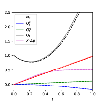
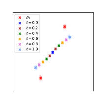
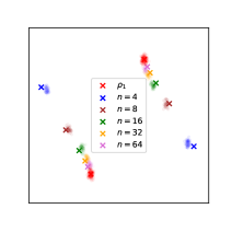
Figure 2: In all three plots, $\lambda=0.1,\alpha(t)=1-t,\beta(t)=t,\varphi=\mathrm{sign}$. (left) $\sigma=1.5,n=8.$ Temporal evolution of the summary statistics $M_{t},Q^{\xi}_{t},Q^{\eta}_{t},Q_{t},\bm{X}_{t}\angle\bm{\mu}$ (15). Solid lines correspond to the theoretical prediction of (15) in Result III.1, while dashed lines correspond to numerical simulations of the generative model, by discretizing the differential equation (7) with step size $\delta t=0.01$, and training a separate DAE for each time step using Adam with learning rate $0.01$ for $2000$ epochs. All experiments were conducted in dimension $d=5000$, and a single run is represented. (middle) $\sigma=2,n=16$. PCA projection of the distribution of $\bm{X}_{t}$ (7), transported by the velocity field $\hat{\bm{b}}$ (6) learnt from data. The point clouds correspond to numerical simulations. Crosses correspond to the theoretical prediction of the means of the cluster, as given by equation (16) of Result III.1. The target Gaussian mixture $\rho_{1}$ is represented in red. The base zero-mean Gaussian density $\rho_{0}$ (dark blue) is split by the flow (7) into two clusters, which approach the target clusters (red) as time accrues . (right) $\sigma=2$. PCA visualization of the generated density $\hat{\rho}_{1}$, by training the generative model on $n$ samples, for $n\in\{4,8,16,32,64\}$. Point clouds represent numerical simulations of the generative model. Crosses represent the theoretical predictions of Result III.1 for the means of the clusters of $\hat{\rho}_{1}$, as given by equation (16) of Result III.1 for $t=1$. As the number of training samples $n$ increases, the generated clusters of $\hat{\rho}_{1}$ approach the target clusters of $\rho_{1}$, represented in red.

Equations (20),(21) and (22) of Remark III.2 are consistent discretizations of the continuous flows (16),(17) and (18) of Result III.1 respectively, and converge thereto in the limit of small discretization steps $\max_{k}\delta t_{k}\to 0$. A derivation of Remark III.2 is detailed in Appendix B. An important consequence of Result III.1 is that the transport of a sample $\bm{X}_{0}\sim\rho_{0}$ by (7) factorizes into the low-dimensional deterministic evolution of its projection on the low-rank subspace $\mathrm{span}(\bm{\mu},\bm{\xi},\bm{\eta})$, as tracked by the three summary statistics $M_{t},Q^{\xi}_{t},Q^{\eta}_{t}$, and the simple linear dynamics of its projection on the orthogonal space $\mathrm{span}(\bm{\mu},\bm{\xi},\bm{\eta})^{\perp}$. Result III.1 thus reduces the high-dimensional flow (7) into a set of three scalar ordinary differential equations (16) and a simple homogeneous linear differential equation (17). The theoretical predictions of Result (III.1) and Remark III.2 for the summary statistics $M_{t},Q^{\xi}_{t},Q^{\eta}_{t},Q_{t}$ are plotted in Fig. 2, and display convincing agreement with numerical simulations, corresponding to discretizing the flow (7) in $N=100$ time steps, and training a separate network for each step as described in Section I. A PCA visualization of the flow is further provided in Fig. 2 (middle).

Leveraging the simple characterization of Result III.1, one is now in a position to characterize the generated distribution $\hat{\rho}_{1}$, which is the density effectively sampled by the generative model. In particular, Result III.1 establishes that the distribution $\hat{\rho}_{1}$ is Gaussian over $\mathrm{span}(\bm{\mu},\bm{\xi},\bm{\eta})^{\perp}$ – since $\bm{X}_{0}^{\perp}$ is Gaussian and the flow is linear–, while the density in $\mathrm{span}(\bm{\mu},\bm{\xi},\bm{\eta})$ concentrates along the vector $\hat{\bm{\mu}}$ described by the components (16). The density $\hat{\rho}_{1}$ is thus described by a mixture of two clusters, Gaussian along $d-3$ directions, centered around $\pm\hat{\bm{\mu}}$. The following corollary provides a sharp characterization of the squared distance between the mean $\hat{\bm{\mu}}$ of the generated density $\hat{\rho}_{1}$ and the true mean $\bm{\mu}$ of the target density $\rho_{1}$.

Corollary III.3.

(Mean squared error of the mean estimate) Let $\hat{\bm{\mu}}$ be the cluster mean of the density $\hat{\rho}_{1}$ generated by the (continuous) learnt flow (7). In the asymptotic limit described by Result II.1, the squared distance between $\hat{\bm{\mu}}$ and the true mean $\bm{\mu}$ is given by

$$\frac{1}{d}\lVert\hat{\bm{\mu}}-\bm{\mu}\lVert^{2}=M_{1}^{2}+n(Q_{1}^{\xi})^{2}+n\sigma^{2}(Q_{1}^{\eta})^{2}+1-2M_{1},$$ (23)

with $M_{1},Q^{\xi}_{1},Q^{\eta}_{1}$ being the solutions of the ordinary differential equations (16) evaluated at time $t=1$. Furthermore, the cosine similarity between $\hat{\bm{\mu}}$ and the true mean $\bm{\mu}$ is given by

$$\hat{\bm{\mu}}\angle\bm{\mu}=\frac{M_{1}}{\sqrt{Q_{1}}}.$$ (24)

Finally, both the Mean Squared Error (MSE) $\nicefrac{{1}}{{d}}\lVert\hat{\bm{\mu}}-\bm{\mu}\lVert^{2}$ (23) and the cosine asimilarity $1-\hat{\bm{\mu}}\angle\bm{\mu}$ (24) decay as $\Theta_{n}(\nicefrac{{1}}{{n}})$ for large number of samples $n$.

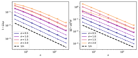
Figure 3: $\alpha(t)=1-t,\beta(t)=t,\varphi=\mathrm{sign}$. Cosine asimilarity (left) and mean squared distance (right) between the mean $\hat{\bm{\mu}}$ of the generated mixture $\hat{\rho}_{1}$ and the mean $\bm{\mu}$ of the target density $\rho_{1}$, as a function of the number of training samples $n$, for various variances $\sigma$ of $\rho_{1}$. Solid lines represent the theoretical characterization of Corollary III.3. Crosses represent numerical simulations of the generative model, by discretizing the differential equation (7) with step size $\delta t=0.01$, and training a separate DAE for each time step using the Pytorch implementation of the full-batch Adam optimizer, with learning rate $0.04$ and weight decay $\lambda=0.1$ for $6000$ epochs. All experiments were conducted in dimension $d=5\times 10^{4}$, and a single run is represented. Dashed lines indicate the performance of the Bayes-optimal estimator $\hat{\bm{\mu}}^{\star}$, as theoretically characterized in Remark IV.1. Dots indicate the performance of the PCA estimator, which is found as in [11] to yield performances nearly identical to the Bayes-optimal estimator.

The heuristic derivation of Corollary III.3 is presented in Appendix A.1. The theoretical predictions of the learning metrics (23) and (24) are plotted in Fig. 3 as a function of the number of samples, along with the corresponding numerical simulations, and display a clear $\Theta_{n}(\nicefrac{{1}}{{n}})$ decay, signalling the convergence of the generated density $\hat{\rho}_{1}$ to the true target density $\rho_{1}$ as the sample complexity accrues. A PCA visualization of this convergence is further presented in Fig.2 (right).

IV Bayes-optimal baseline

Corollary III.3 completes the study of the performance of the DAE-parametrized generative model. It is natural to wonder whether one can improve on the $\Theta_{n}(\nicefrac{{1}}{{n}})$ rate that it achieves. A useful baseline to compare with is the Bayes-optimal estimator $\hat{\bm{\mu}}^{\star}$, yielded by Bayesian inference when in addition to the dataset $\mathcal{D}=\{\bm{x}_{1}^{\mu}\}_{\mu=1}^{n}$, the form of the distribution (8) and the variance $\sigma$ are known, but not the mean $\bm{\mu}$ –which for definiteness and without loss of generality will be assumed in this section to be have been drawn at random from $\mathcal{N}(0,\mathbb{I}_{d})$. The following remark provides a tight characterization of the MSE achieved by this estimator.

Remark IV.1.

(Bayes-optimal estimator of the cluster mean) The Bayes-optimal estimator $\hat{\bm{\mu}}^{\star}$ of $\bm{\mu}$ assuming knowledge of the functional form of the target density (8), the cluster variance $\sigma$, and the training set $\mathcal{D}$, is defined as the minimizer of the average squared error

$$\hat{\bm{\mu}}^{\star}=\underset{\nu}{\mathrm{arginf}}\mathbb{E}_{\bm{\mu}\sim\mathcal{N}(0,\mathbb{I}_{d}),\mathcal{D}\sim\rho_{1}^{\otimes n}}\lVert\nu(\mathcal{D})-\bm{\mu}\lVert^{2}.$$ (25)

In the asymptotic limit of Result II.1, the Bayes-optimal estimator $\hat{\bm{\mu}}^{\star}(\mathcal{D})$ is contained in $\mathrm{span}(\bm{\mu},\bm{\eta})$, where $\bm{\eta}$ was defined in equation (12) in Result II.1. Its components

$$m^{\star}\equiv\frac{\bm{\mu}^{\top}\hat{\bm{\mu}}^{\star}(\mathcal{D})}{d}, q^{\star}_{\eta}\equiv\frac{\bm{\eta}^{\top}\hat{\bm{\mu}}^{\star}(\mathcal{D})}{nd\sigma^{2}},$$ (26)

concentrate asymptotically to

$$m^{\star}=\frac{n}{n+\sigma^{2}}, q^{\star}_{\eta}=\frac{1}{n+\sigma^{2}}.$$ (27)

Finally, with high probability, the Bayes-optimal MSE reads

$$\frac{1}{d}\lVert\hat{\bm{\mu}}^{\star}(\mathcal{D})-\bm{\mu}\lVert^{2}=\frac{\sigma^{2}}{n+\sigma^{2}}.$$ (28)

In particular, (28) implies that the optimal MSE decays as $\Theta_{n}(\nicefrac{{1}}{{n}})$.

Remark IV.1, whose derivation is detailed in Appendix C, thus establishes that the Bayes-optimal MSE decays as $\Theta_{n}(\nicefrac{{1}}{{n}})$ with the number of available training samples. Contrasting to Corollary III.3 for the MSE associated to the mean $\hat{\bm{\mu}}$ of the density $\hat{\rho}_{1}$ learnt by the generative model, it follows that the latter achieves the Bayes-optimal learning rate. The Bayes-optimal MSE (28) predicted by Remark IV.1 is plotted in dashed lines in Fig. 3, alongside the MSE achieved by the generative model (see Corollary III.3). The common $\nicefrac{{1}}{{n}}$ decay rate is also plotted in dashed black for comparison. Finally, we observe that the estimate of $\bm{\mu}$ inferred by PCA, plotted as dots in Fig. 3, leads to a cosine similarity which is very close to the Bayes-optimal one, echoing the findings of [11] in another asymptotic limit. We however stress an important distinction between the generative model analyzed in previous sections and the Bayes and PCA estimators dicussed in the present section. The generative model is tasked with estimating the full distribution $\rho_{1}$ only from data, while being completely agnostic thereof. In contrast, PCA and Bayesian inference only offer an estimate of the cluster mean, and require an exact oracle knowledge of its functional form (8) and the cluster variance $\sigma$. They do not, therefore, constitute generative models and are only discussed in the present section as insightful baselines.

It is a rather striking finding that that the DAE (9) succeeds in approximately sampling from $\rho_{1}$(8) when trained on but $n=\Theta_{d}(1)$ samples –instead of simply generating back memorized training samples–, and further displays information-theoretically optimal learning rates. The answer to this puzzle, which we briefly discussed in the introduction, lies in the fact that the architecture (9) is very close to the functional form of the exact velocity field $b$ (1), as further detailed in Appendix B (see (68)), and is therefore implicitly biased towards learning the latter – while also not being expressive enough to too detrimentally overfit. This architecture-induced bias towards the correct flow can alternatively be viewed as a form of implicit regularization inherited from the network parametrization of the velocity field. These observations bring preliminary answers, at least in the present setting, to the interrogation raised in the introduction on the unreasonnable effectiveness of generative models. The exploration of the tradeoff between the network expressivity and architectural bias with the performance of the generative model in more complex settings is an important and fascinating entreprise, which is left for future work.

Conclusion

We conduct a tight end-to-end asymptotic analysis of estimating and sampling a binary Gaussian mixture using a flow-based generative model, when the flow is parametrized by a shallow auto-encoder. We provide sharp closed-form characterizations for the trained weights of the network, the learnt velocity field, a number of summary statistics tracking the generative flow, and the distance between the mean of the generated mixture and the mean of the target mixture. The latter is found to display a $\Theta_{n}(\nicefrac{{1}}{{n}})$ decay rate, where $n$ is the number of samples, which is further shown to be the Bayes-optimal rate. In contrast to most studies of flow-based generative models in high dimensions, the learning and sampling processes are jointly and sharply analyzed in the present manuscript, which affords the possibility to explicitly investigate the effect of a limited sample complexity at the level of the generated density. Our findings shed preliminary light on the role of the network-induced implicit regularization in the unreasonable effectiveness of generative models in generating new samples –instead of merely memorizing training samples.

Acknowledgement

We thank Michael Albergo, Nicholas Boffi, Arthur Jacot and Ahmed El Alaoui for insightful discussions. Part of this work was done during HC’s visit in the Courant Institute in March 2023. We acknowledge funding from the Swiss National Science Foundation grants OperaGOST (grant number 200390) and SMArtNet (grant number 212049). EVE is supported by the National Science Foundation under awards DMR-1420073, DMS-2012510, and DMS-2134216, by the Simons Collaboration on Wave Turbulence, Grant No. 617006, and by a Vannevar Bush Faculty Fellowship.

Appendix A Derivation of Result II.1

In this appendix, we detail the heuristic derivation of Result (II.1), which provides a sharp asymptotic characterization of the parameters $\hat{c}_{t},\hat{w}_{t}$ of the DAE (9) minimizing the time $t$ risk $\hat{\mathcal{R}}_{t}$ (10). In the following, the time index $t\in[0,1]$ is considered fixed.

In order to characterize observables depending on the minimizers $\hat{c}_{t},\hat{w}_{t}$ of the risk $\hat{\mathcal{R}}_{t}$ (10), observe that for any test function $\phi(c_{t},w_{t})$:

$$\phi(\hat{c}_{t},\hat{w}_{t})=\underset{\gamma\to\infty}{\lim}\frac{1}{Z}\int dwdc\phi(c,w)e^{-\gamma\mathcal{\hat{R}}_{t}(w,c)},$$ (29)

where the normalization $Z$ is

$$\mathcal{Z}\left(\mathcal{D}\right)=\int dc~{}dwe^{-\frac{\gamma}{2}\left\lVert x_{1}^{\mu}-\left[c\times(\beta(t)x_{1}^{\mu}+\alpha(t)x_{0}^{\mu})+w\varphi\left(w^{\top}(\beta(t)x_{1}^{\mu}+\alpha(t)x_{0}^{\mu})\right)\right]\right\rVert^{2}-\frac{\gamma\lambda}{2}\|w\rVert^{2}}.$$ (30)

We emphasized the dependence on the train set $\mathcal{D}=\{x_{0}^{\mu},x_{t}^{\mu}\}_{\mu=1}^{n}$. $\ln Z(\mathcal{D})$ can then be studied as a moment generating function, and integrals of the form (29) deduced therefrom. In the following, we therefore seek to establish an asymptotic characterization of $\ln Z(\mathcal{D})$.

An important observation lies in the fact that the argument $w^{\top}x$ of the activation $\varphi$ of the DAE is expected in high dimensions $d\to\infty$ to be very large. In particular, we shall self-consistently establish that it is more precisely scaling like $\Theta_{d}(d)$. As a result, only the asymptotic behaviour in $\pm\infty$ of $\varphi$ matters, and by assumption $\varphi(w^{\top}x)\approx\mathrm{sign}(w^{\top}x)$ asymptotically. We shall therefore self-consistently take $\varphi=\mathrm{sign}$ in the following.

A.1 Computation of the partition function

In the following, for clarity, we use the decomposition $x_{1}^{\mu}=s^{\mu}\mu+z^{\mu}$, introduced below (8) in the main text, with $s^{\mu}\in\{-1,+1\}$ and $z^{\mu}\sim\mathcal{N}(0,\sigma^{2}\mathbb{I}_{d})$. Under these notations, the partition function reads:

$$\mathcal{Z}(\mathcal{D})= \int dc~{}dwe^{{\scriptscriptstyle-\frac{\gamma d}{2}\sum\limits_{\mu=1}^{n}\frac{\lVert w\rVert^{2}}{d}\mathrm{sign}\left(w^{\top}(\beta(t)(s^{\mu}\mu+z^{\mu})+\alpha(t)x_{0}^{\mu})\right)^{2}}}$$

$$\times e^{{\scriptscriptstyle\gamma d\sum\limits_{\mu=1}^{n}\mathrm{sign}\left(w^{\top}(\beta(t)(s^{\mu}\mu+z^{\mu})+\alpha(t)x_{0}^{\mu})\right)\frac{w^{\top}((1-c\beta(t))(s^{\mu}\mu+z^{\mu})-c\alpha(t)x_{0}^{\mu})}{d}}}\times e^{-\frac{\gamma\lambda}{2}\lVert w\lVert^{2}}$$

$$\times e^{{\scriptscriptstyle-\frac{\gamma d}{2}\sum\limits_{\mu=1}^{n}\left[(1-\beta(t)c)^{2}\frac{\lVert\mu^{\mu}\rVert^{2}+\lVert z^{\mu}\rVert^{2}+2s^{\mu}\mu^{\top}z^{\mu}}{d}+c^{2}\frac{\lVert\alpha(t)x_{0}^{\mu}\rVert^{2}}{d}+2b(\beta(t)c-1)\frac{s^{\mu}\mu^{\top}\alpha(t)x_{0}^{\mu}+\eta^{\mu\top}\alpha(t)x_{0}^{\mu}}{d}\right]}}$$ (31)

Note that we benignly introduced a $\nicefrac{{1}}{{d}}$ factor inside the sign function $\mathrm{sign}$. One is now in position to introduce the overlaps

$$q\equiv\frac{\lVert w\lVert^{2}}{2}, q_{\xi}^{\mu}\equiv s^{\mu}\frac{w^{\top}x_{0}^{\mu}}{d}, q_{\eta}^{\mu}\equiv s^{\mu}\frac{w^{\top}z^{\mu}}{d}, m\equiv\frac{w^{\top}\mu}{d}.$$ (32)

Note that because of $n=\Theta(1)$ there is a finite number of these such overlaps. Besides, note that our starting assumption that the argument $w^{\top}x$ of the activation $\varphi$ is $\Theta_{d}(d)$ translates into the fact that all these order parameters should be $\Theta_{d}(1)$, which we shall self-consistently show to be indeed the case. The partition function then reads

$$\mathcal{Z}(\mathcal{D})= \int dc~{}dmd\hat{m}~{}dqd\hat{q}\prod\limits_{\mu=1}^{n}d\hat{d}q_{\eta}^{\mu}d\hat{q}_{\eta}^{\mu}~{}dq_{\xi}^{\mu}e^{\frac{d}{2}\hat{q}q+d\hat{m}m+d\sum\limits_{\mu=1}^{n}(\hat{q}_{\xi}^{\mu}q_{\xi}^{\mu}+\hat{q}_{\eta}^{\mu}q_{\eta}^{\mu})}$$

$$\int dwe^{-\frac{\gamma\lambda}{2}\lVert w\lVert^{2}-\frac{\hat{q}}{2}\lVert w\lVert^{2}-\left(\hat{m}\mu+\sum\limits_{\mu=1}^{n}(\hat{q}_{\xi}^{\mu}s^{\mu}x_{0}^{\mu}+\hat{q}_{\eta}^{\mu}s^{\mu}z^{\mu})\right)^{\top}w}e^{\scriptscriptstyle-\frac{\gamma d}{2}\sum\limits_{\mu=1}^{n}\left[(1+\sigma^{2})(1-\beta(t)c)^{2}+c^{2}\alpha(t)^{2}\right]}$$

$$e^{{\scriptscriptstyle-\frac{\gamma d}{2}\sum\limits_{\mu=1}^{n}\left[q\mathrm{sign}\left(\beta(t)(m+q_{\eta}^{\mu})+\alpha(t)q^{\mu}_{\xi}\right)^{2}-2\mathrm{sign}\left(\beta(t)(m+q_{\eta}^{\mu})+\alpha(t)q^{\mu}_{\xi}\right)\left[(1-c\beta(t))(m+q^{\mu}_{\eta})-c\alpha(t)q_{\xi}^{\mu}\right]\right]}}.$$ (33)

Therefore

$$\mathcal{Z}(\mathcal{D})= \int dc~{}dmd\hat{m}~{}dqd\hat{q}\prod\limits_{\mu=1}^{n}d\hat{q}_{\xi}^{\mu}dq_{\eta}^{\mu}d\hat{q}_{\eta}^{\mu}~{}dq_{\xi}^{\mu}$$

$$e^{\frac{d}{2}\hat{q}q+d\hat{m}m+d\sum\limits_{\mu=1}^{n}(\hat{q}_{\xi}^{\mu}q_{\xi}^{\mu}+\hat{q}_{\eta}^{\mu}q_{\eta}^{\mu})+\frac{d}{2(\gamma\lambda+\hat{q})}\frac{1}{d}\left\lVert\hat{m}\mu+\sum\limits_{\mu=1}^{n}(\hat{q}_{\xi}^{\mu}s^{\mu}x_{0}^{\mu}+\hat{q}_{\eta}^{\mu}s^{\mu}z^{\mu})\right\lVert^{2}}$$

$$e^{{\scriptscriptstyle-\frac{\gamma d}{2}\sum\limits_{\mu=1}^{n}\left[q\mathrm{sign}\left(\beta(t)(m+q_{\eta}^{\mu})+\alpha(t)q^{\mu}_{\xi}\right)^{2}-2\mathrm{sign}\left(\beta(t)(m+q_{\eta}^{\mu})+\alpha(t)q^{\mu}_{\xi}\right)\left[(1-c\beta(t))(m+q^{\mu}_{\eta})-c\alpha(t)q_{\xi}^{\mu}\right]\right]}}$$

$$e^{{\scriptscriptstyle-\frac{\gamma d}{2}\sum\limits_{\mu=1}^{n}\left[(1+\sigma^{2})(1-\beta(t)c)^{2}+c^{2}\alpha(t)^{2}\right]}-\frac{d}{2}\ln(\gamma\lambda+\hat{q})}.$$ (34)

The last term in the first exponent can be further simplified as

$$\frac{1}{d}\left\lVert\hat{m}\mu+\sum\limits_{\mu=1}^{n}(\hat{q}_{\xi}^{\mu}s^{\mu}x_{0}^{\mu}+\hat{q}_{\eta}^{\mu}s^{\mu}z^{\mu})\right\lVert^{2} =\hat{m}^{2}+\sum\limits_{\mu=1}^{n}\left[(\hat{q}_{\xi}^{\mu})^{2}+(\hat{q}_{\eta}^{\mu})^{2}\sigma^{2}\right]$$

$$~{}~{}~{}+2\sum\limits_{\mu=1}^{n}\left[\hat{q}_{\xi}^{\mu}s^{\mu}\frac{\mu^{\top}x_{0}^{\mu}}{d}+\hat{q}_{\eta}^{\mu}s^{\mu}\frac{\mu^{\top}z^{\mu}}{d}\right]$$

$$~{}~{}~{}+\sum\limits_{\mu,\nu=1}^{n}s^{\mu}s^{\nu}\left[\scriptstyle\hat{q}_{\xi}^{\mu}\hat{q}_{\xi}^{\nu}\frac{(x_{0}^{\nu})\top x_{0}^{\mu}}{d}+\hat{q}_{\eta}^{\nu}\hat{q}_{\eta}^{\mu}\frac{(z^{\nu})^{\top}z^{\mu}}{d}+\hat{q}_{\xi}^{\mu}\hat{q}_{\eta}^{\nu}\frac{(z^{\nu})^{\top}x_{0}^{\mu}}{d}\right]$$

$$=\hat{m}^{2}+\sum\limits_{\mu=1}^{n}\left[(\hat{q}_{\xi}^{\mu})^{2}+(\hat{q}_{\eta}^{\mu})^{2}\sigma^{2}\right]+\mathcal{O}\left(\nicefrac{{1}}{{\sqrt{d}}}\right),$$ (35)

with the last line holding with high probability, using the fact that since $z,x_{0}$ are two independently drawn standard Gaussian vectors $\nicefrac{{z^{\top}x_{0}}}{{d}}=\Theta_{d}(\nicefrac{{1}}{{\sqrt{d}}})$ with high probability. Finally,

$$\mathcal{Z}(\mathcal{D})= \int dc~{}dmd\hat{m}~{}dqd\hat{q}\prod\limits_{\mu=1}^{n}d\hat{q}_{\xi}^{\mu}dq_{\eta}^{\mu}d\hat{q}_{\eta}^{\mu}~{}dq_{\xi}^{\mu}$$

$$e^{\frac{d}{2}\hat{q}q+d\hat{m}m+d\sum\limits_{\mu=1}^{n}(\hat{q}_{\xi}^{\mu}q_{\xi}^{\mu}+\hat{q}_{\eta}^{\mu}q_{\eta}^{\mu})+\frac{d}{2(\gamma\lambda+\hat{q})}\left[\hat{m}^{2}+\sum\limits_{\mu=1}^{n}\left[(\hat{q}_{\xi}^{\mu})^{2}+(\hat{q}_{\eta}^{\mu})^{2}\sigma^{2}\right]\right]}$$

$$e^{{\scriptscriptstyle-\frac{\gamma d}{2}\sum\limits_{\mu=1}^{n}\left[q\mathrm{sign}\left(\beta(t)(m+q_{\eta}^{\mu})+\alpha(t)q^{\mu}_{\xi}\right)^{2}-2\mathrm{sign}\left(\beta(t)(m+q_{\eta}^{\mu})+\alpha(t)q^{\mu}_{\xi}\right)\left[(1-c\beta(t))(m+q^{\mu}_{\eta})-c\alpha(t)q_{\xi}^{\mu}\right]\right]}{\scriptscriptstyle}}$$

$$e^{\scriptstyle-\frac{\gamma d}{2}\sum\limits_{\mu=1}^{n}\left[(1+\sigma^{2})(1-\beta(t)c)^{2}+c^{2}\alpha(t)^{2}\right]-\frac{d}{2}\ln(\gamma\lambda+\hat{q})}$$ (36)

Since all the terms in the exponent of the integrand scale like $d$, in the asymptotic limit $d\to\infty$ the integral can be computed using a Laplace approximation.

A.2 Sample-symmetric ansatz

The partition function is given by taking the saddle point in (A.1). This involves a maximization problem over $4n+5$ variables. Note that since $n=\Theta_{d}(1)$, this is a low dimensional – thus a priori tractable – optimization problem, but which nevertheless remains cumbersome. However, the symmetries of the problem make it possible to determine the form of the maximizer, and thus drastically simplify the optimization problem. Note that indeed, asymptotically, the vectors $\mu,\{x_{0}^{\mu},z^{\mu}\}_{\mu=1}^{n}$ involved in the definition of the overlaps $m,\{q_{\xi}^{\mu},q_{\eta}^{\mu}\}_{\mu=1}^{n}$ (32) are all mutually asymptotically orthogonal – i.e. they have vanishing cosine similarity. Therefore, the parameters $m,\{q_{\xi}^{\mu},q_{\eta}^{\mu}\}_{\mu=1}^{n}$ can be considered as independent variables. Since furthermore all the samples play interchangeable roles in high dimensions – in that all data points are asymptotically at the same angle with the cluster mean $\mu$, which is the only relevant direction of the problem–, one can look for the saddle point assuming the symmetric ansatz

$$\forall\mu,~{}q^{\mu}_{\xi}=q_{\xi},~{}~{}\hat{q}^{\mu}_{\xi}=\hat{q}_{\xi},$$ (37)

$$\forall\mu,~{}~{}q^{\mu}_{\eta}=q_{\eta},~{}~{}\hat{q}^{\mu}_{\eta}=\hat{q}_{\eta}.$$ (38)

This ansatz is further validated in numerical experiments, when training a DAE with the Pytorch implementation of the Adam optimizer. Under this ansatz, the partition function reduces to

$$\mathcal{Z}(\mathcal{D} )=\int dc~{}dmd\hat{m}~{}dqd\hat{q}d\hat{q}_{\xi}dq_{\eta}d\hat{q}_{\eta}dq_{\xi}e^{\frac{d}{2}\hat{q}q+d\hat{m}m+dn(\hat{q}_{\xi}q_{\xi}+\hat{q}_{\eta}q_{\eta})+\frac{d}{2(\gamma\lambda+\hat{q})}\left[\hat{m}^{2}+n(\hat{q}_{\xi}^{2}+\hat{q}_{\eta}^{2}\sigma^{2})\right]}$$

$$e^{{\scriptscriptstyle-\frac{\gamma d}{2}n\left[q\mathrm{sign}\left(\beta(t)(m+q_{\eta})+\alpha(t)q_{\xi}\right)^{2}-2\mathrm{sign}\left(\beta(t)(m+q_{\eta})+\alpha(t)q_{\xi}\right)\left[(1-c\beta(t))(m+q_{\eta})-c\alpha(t)q_{\xi}\right]+(1+\sigma^{2})(1-\beta(t)c)^{2}+c^{2}\alpha(t)^{2}\right]}}$$

$$e^{-\frac{d}{2}\ln(\gamma\lambda+\hat{q})}$$ (39)

Note that the exponent is now independent of the dataset $\mathcal{D}$. In other words, in the regime $d\to\infty,n=\Theta_{d}(1)$, the log partition function concentrates with respect to the randomness associated with the sampling of the training set. The effective action (log partition function) therefore reads

$$\ln\mathcal{Z}(\mathcal{D})= \underset{c,\hat{q},q,\hat{m},m,\hat{q}_{\eta,\xi},q_{\eta,\xi}}{\mathrm{extr}}\frac{1}{2}\hat{q}q+\hat{m}m+n(\hat{q}_{\xi}q_{\xi}+\hat{q}_{\eta}q_{\eta})+\frac{1}{2(\gamma\lambda+\hat{q})}\left[\hat{m}^{2}+n(\hat{q}_{\xi}^{2}+\hat{q}_{\eta}^{2}\sigma^{2})\right]$$

$$-\frac{\alpha}{2}n\left[\scriptstyle q\mathrm{sign}\left(\beta(t)(m+q_{\eta})+\alpha(t)q_{\xi}\right)^{2}-2\mathrm{sign}\left(\beta(t)(m+q_{\eta})+\alpha(t)q_{\xi}\right)\left[(1-c\beta(t))(m+q_{\eta})-c\alpha(t)q_{\xi}\right]\right]$$

$$-\frac{\gamma n}{2}\left[(1+\sigma^{2})(1-\beta(t)c)^{2}+c^{2}\alpha(t)^{2}\right]-\frac{1}{2}\ln(\gamma\lambda+\hat{q})$$ (40)

This expression has to be extremized with respect to $c,\hat{q},q,\hat{m},m,\hat{q}_{\eta,\xi},q_{\eta,\xi}$ in the $\gamma\to\infty$ limit. Rescaling the conjugate variables as

$$\gamma\hat{q}\leftarrow\hat{q}, \gamma\hat{q}_{\eta,\xi}\leftarrow\hat{q}_{\eta,\xi}, \gamma\hat{m}\leftarrow\hat{m}$$ (41)

the action becomes, in the $\gamma\to\infty$ limit (changing for readability the conjugates $\hat{m},\hat{q}_{\eta,\xi}\to-\hat{m},-\hat{q}_{\eta,\xi}$):

$$\ln\mathcal{Z}(\mathcal{D})= \underset{c,\hat{q},q,\hat{m},m,\hat{q}_{\eta,\xi},q_{\eta,\xi}}{\mathrm{extr}}\frac{1}{2}\hat{q}q-\hat{m}m-n(\hat{q}_{\xi}q_{\xi}+\hat{q}_{\eta}q_{\eta})+\frac{1}{2(\lambda+\hat{q})}\left[\hat{m}^{2}+n(\hat{q}_{\xi}^{2}+\hat{q}_{\eta}^{2}\sigma^{2})\right]$$

$$-\frac{n}{2}\left[\scriptstyle q\mathrm{sign}\left(\beta(t)(m+q_{\eta})+\alpha(t)q_{\xi}\right)^{2}-2\mathrm{sign}\left(\beta(t)(m+q_{\eta})+\alpha(t)q_{\xi}\right)\left[(1-c\beta(t))(m+q_{\eta})-c\alpha(t)q_{\xi}\right]\right]$$

$$-\frac{n}{2}\left[(1+\sigma^{2})(1-\beta(t)c)^{2}+c^{2}\alpha(t)^{2}\right]$$ (42)

A.3 Saddle-point equations

The extremization of $\ln\mathcal{Z}(\mathcal{D})$ can be alternatively written as zero-gradient equations on each of the parameters the extremization is carried over, yielding

$$\begin{cases}q=\frac{\hat{m}^{2}+n(\hat{q}_{\xi}^{2}+\hat{q}_{\eta}^{2}\sigma^{2})}{(\lambda+\hat{q})^{2}}\\ m=\frac{\hat{m}}{\lambda+\hat{q}}\\ q_{\xi}=\frac{\hat{q}_{\xi}}{\lambda+\hat{q}}\\ q_{\eta}=\frac{\hat{q}_{\eta}\sigma^{2}}{\lambda+\hat{q}}\end{cases} \begin{cases}\nu\equiv\beta(t)(m+q_{\eta})+\alpha(t)q_{\xi}\\ \hat{q}=n\\ \hat{m}=n\mathrm{sign}(\nu)(1-c\beta(t))\\ \hat{q}_{\eta}=\frac{\hat{m}}{n}\\ \hat{q}_{\xi}=-c\alpha(t)\mathrm{sign}(\nu)\\ c=\frac{(1+\sigma^{2})\beta(t)-\mathrm{sign}(\nu)(\beta(t)(m+q_{\eta})+\alpha(t)q_{\xi})}{\alpha(t)^{2}+\beta(t)^{2}(1+\sigma^{2})}\end{cases}$$ (43)

Note the identity

$$q=m^{2}+n(q_{\xi}^{2}+\nicefrac{{q_{\eta}^{2}}}{{\sigma^{2}}})$$ (44)

which follows from the asymptotic orthogonality of the vectors and the Pythagorean theorem. This implies in particular that the square norm of $\hat{w}$, as measure by $q$, is only the sum of its projections along $\mu$ (corresponding to $m$) $\xi$ (corresponding to $q_{\xi}$) and $\eta$ ($q_{\eta}$). Therefore, the norm of the orthogonal projection of $\hat{w}$ with respect to $\mathrm{span}(\mu,\eta,\xi)$ is asymptotically vanishing. In other words, $\hat{w}$ is asymptotically contained in $\mathrm{span}(\mu,\eta,\xi)$.

Remark that the symmetry $m,\hat{m},q_{\eta,\xi},\hat{q}_{\eta,\xi}\to-m,-\hat{m},-q_{\eta,\xi},-\hat{q}_{\eta,\xi}$ leaves equations (43) unchanged, meaning that if $m,\hat{m},q_{\eta,\xi},\hat{q}_{\eta,\xi}$ is a solution to the saddle-point equations, so is $m,\hat{m},q_{\eta,\xi},\hat{q}_{\eta,\xi}$. This is due to the symmetry between the clusters in the target density (8), as $\mu\to-\mu$ yields the same model. As a convention, we can thus suppose without loss of generality $\nu\geq 0$ in (43). (43) then simplifies to

$$\begin{cases}q=\frac{\hat{m}^{2}+n(\hat{q}_{\xi}^{2}+\hat{q}_{\eta}^{2}\sigma^{2})}{(\lambda+\hat{q})^{2}}\\ m=\frac{\hat{m}}{\lambda+\hat{q}}\\ q_{\xi}=\frac{\hat{q}_{\xi}}{\lambda+\hat{q}}\\ q_{\eta}=\frac{\hat{q}_{\eta}\sigma^{2}}{\lambda+\hat{q}}\end{cases} \begin{cases}\hat{q}=n\\ \hat{m}=n(1-c\beta(t))\\ \hat{q}_{\eta}=\frac{\hat{m}}{n}\\ \hat{q}_{\xi}=-\alpha(t)c\\ c=\frac{(1+\sigma^{2})\beta(t)-(\beta(t)(m+q_{\eta})+\alpha(t)q_{\xi})}{\alpha(t)^{2}+\beta(t)^{2}(1+\sigma^{2})}\end{cases}.$$ (45)

The skip connection strength $c$ thus satisfies the self-consistent equation

$$c=\frac{(1+\sigma^{2})\beta(t)-\frac{1}{\lambda+n}(\beta(t)(1-\beta(t)c)(n+\sigma^{2})-\alpha(t)^{2}c)}{\alpha(t)^{2}+\beta(t)^{2}(1+\sigma^{2})},$$ (46)

which can be solved as

$$c=\frac{\beta(t)(\lambda(1+\sigma^{2})+(n-1)\sigma^{2})}{\alpha(t)^{2}(\lambda+n-1)+\beta(t)^{2}(\lambda(1+\sigma^{2})+(n-1)\sigma^{2})}$$ (47)

which recovers equation (11) of Result II.1. Plugging this expression back to (45), and redefining $\sigma^{2}q_{\eta}\leftarrow q_{\eta}$, yields

$$\begin{cases}m_{t}=\frac{n}{\lambda+n}\frac{\alpha(t)^{2}(\lambda+n-1)}{\alpha(t)^{2}(\lambda+n-1)+\beta(t)^{2}(\lambda(1+\sigma^{2})+(n-1)\sigma^{2})}\\ q_{t}^{\eta}=\frac{\sigma^{2}}{\lambda+n}\frac{\alpha(t)^{2}(\lambda+n-1)}{\alpha(t)^{2}(\lambda+n-1)+\beta(t)^{2}(\lambda(1+\sigma^{2})+(n-1)\sigma^{2})}\\ q_{t}^{\xi}=-\frac{1}{\lambda+n}\frac{\alpha(t)\beta(t)(\lambda(1+\sigma^{2})+(n-1)\sigma^{2})}{\alpha(t)^{2}(\lambda+n-1)+\beta(t)^{2}(\lambda(1+\sigma^{2})+(n-1)\sigma^{2})}\end{cases}$$ (48)

We have added subscripts $t$ to emphasize the dependence on the time index $t$. Note that for $t>0$, $\nu>0$, which is self-consistent. For $t=0$, $\nu=0$ and the sign function in (43) becomes ill-defined, signalling that the extremum of (A.2) ceases to be a critical point (i.e. differentiable). However, one expects the extremum to still be given by the $t=0$ limit of (43), as there is a priori no singularity in the learning problem for $t=0$. This remark, together with (48), recovers equation (14) from Result II.1. ∎

A.4 Metrics

Result II.1 provides a tight characterization of the skip conneciton strength $\hat{c}_{t}$ and of the vector $\hat{w}_{t}$. The performance of the trained DAE $f_{\hat{c}_{t},\hat{w}_{t}}$ (9) as a denoiser can be further quantified with a number of metrics, for which we also provide sharp asymptotic characterizations below, for completeness.

Result A.1.

(MSE) The test MSE of the learnt denoiser $f_{\hat{c}_{t},\hat{w}_{t}}$ is defined as the test error associated to the risk $\hat{R}_{t}$ (10)

$$\mathrm{mse}_{t}\equiv\mathbb{E}_{x_{1}\sim\rho_{1},x_{0}\sim\rho_{0}}\left\lVert f_{\hat{c}_{t},\hat{w}_{t}}(\alpha(t)x_{0}+\beta(t)x_{1})-x_{1}\right\lVert^{2}.$$ (49)

In the same asymptotic limit as Result II.1 in the main text, this metric is sharply characterized by the closed-form formula

$$\mathrm{mse}_{t}=m_{t}^{2}+n((q_{t}^{\xi})^{2}+(q_{t}^{\eta})^{2}\sigma^{2})-2(1-\hat{c}_{t}\beta(t))m_{t}+(1-\hat{c}_{t}\beta(t))^{2}(1+\sigma^{2})+\hat{c}_{t}^{2}\alpha(t)^{2}$$ (50)

where $\hat{c}_{t},m_{t},q^{\xi}_{t},q^{\eta}_{t}$ were defined in Result II.1. Furthermore, the MSE (49) is lower-bounded by the oracle MSE

$$\mathrm{mse}^{\star}_{t}\equiv\mathbb{E}_{x_{1}\sim\rho_{1},x_{0}\sim\rho_{0}}\left\lVert f_{t}^{\star}(\alpha(t)x_{0}+\beta(t)x_{1})-x_{1}\right\lVert^{2},$$ (51)

where the oracle denoiser follows from an application of Tweedie’s formula [14, 1] as

$$f^{\star}_{t}(x)=\frac{\beta(t)\sigma^{2}}{\alpha(t)^{2}+\beta(t)^{2}\sigma^{2}}x+\frac{\alpha(t)^{2}}{\alpha(t)^{2}+\beta(t)^{2}\sigma^{2}}\mu\times\tanh(\mu^{\top}x).$$ (52)

Finally, the oracle MSE $\mathrm{mse}^{\star}_{t}$ admits the following asymptotic characterization:

$$\mathrm{mse}^{\star}_{t}=\alpha(t)^{4}\sigma^{2}\frac{\alpha(t)^{2}+\sigma^{2}(1-\alpha(t)^{2})}{(\sigma^{2}\beta(t)^{2}+\alpha(t)^{2})^{2}}$$ (53)

Derivation of Result A.1      We begin by detailing the characterizaiton of the DAE MSE (50):

$$\mathrm{mse}_{t} =\frac{1}{d}\mathbb{E}_{x_{1},x_{0}}\langle\left\lVert x_{1}-\left[\hat{c}_{t}\times(\beta(t)x_{1}+\alpha(t)x_{0})+\hat{w}_{t}\mathrm{sign}\left(\hat{w}_{t}^{\top}(\beta(t)x_{1}+\alpha(t)x_{0})\right)\right]\right\rVert^{2}$$

$$=m_{t}^{2}+n((q_{t}^{\xi})^{2}+(q_{t}^{\eta})^{2}\sigma^{2})-2\mathrm{sign}(\beta(t)m_{t})(1-\hat{c}_{t}\beta(t))m_{t}+(1-\hat{c}_{t}\beta(t))^{2}(1+\sigma^{2})+\hat{c}_{t}^{2}\alpha(t)^{2}$$

$$=m_{t}^{2}+n((q_{t}^{\xi})^{2}+(q_{t}^{\eta})^{2}\sigma^{2})-2(1-\hat{c}_{t}\beta(t))m_{t}+(1-\hat{c}_{t}\beta(t))^{2}(1+\sigma^{2})+\hat{c}_{t}^{2}\alpha(t)^{2}$$ (54)

which recovers (50) of Result A.1. (52) follows directly from an application of Tweedie’s formula [14]. The associated MSE (53) can be derived as

$$\mathrm{mse}^{\star} =\frac{\alpha(t)^{4}(1+\sigma^{2})+\sigma^{4}\alpha(t)^{2}(1-\alpha(t)^{2})}{(\sigma^{2}\beta(t)^{2}+\alpha(t)^{2})^{2}}+\frac{\alpha(t)^{4}}{(\sigma^{2}\beta(t)^{2}+\alpha(t)^{2})^{2}}\left[\mathrm{sign}\left(\frac{{\scriptstyle\beta(t)^{2}}}{\sigma^{2}\beta(t)^{2}+\alpha(t)^{2}}\right)^{2}\right]$$

$$-\frac{2\alpha(t)^{2}}{\sigma^{2}\beta(t)^{2}+\alpha(t)^{2}}\left[\mathrm{sign}\left(\frac{{\scriptstyle\beta(t)^{2}}}{\sigma^{2}\beta(t)^{2}+\alpha(t)^{2}}\right)\right]\times\frac{\alpha(t)^{2}}{\sigma^{2}+\alpha(t)^{2}-\sigma^{2}\alpha(t)^{2}}$$

$$=\frac{\alpha(t)^{4}(1+\sigma^{2})+\sigma^{4}\alpha(t)^{2}(1-\alpha(t)^{2})}{(\sigma^{2}\beta(t)^{2}+\alpha(t)^{2})^{2}}-\frac{\alpha(t)^{4}}{(\sigma^{2}\beta(t)^{2}+\alpha(t)^{2})^{2}}=\frac{\alpha(t)^{4}\sigma^{2}+\sigma^{4}\alpha(t)^{2}(1-\alpha(t)^{2})}{(\sigma^{2}\beta(t)^{2}+\alpha(t)^{2})^{2}}$$ (55)

which concludes the derivation of Result A.1∎

Result A.2.

The cosine similarity $\hat{w}_{t}\angle\mu\equiv\nicefrac{{\hat{w}_{t}^{\top}\mu}}{{\lVert\hat{w}_{t}\lVert\lVert\mu\lVert}}$ admits the asymptotic characterization

$$\hat{w}_{t}\angle\mu=\frac{m_{t}}{\sqrt{m_{t}^{2}+n((q_{t}^{\xi})^{2}+(q_{t}^{\eta})^{2}\sigma^{2}}}$$ (56)

where $m_{t},q_{t}^{\xi},q_{t}^{\eta}$ are characterized in Result II.1.

Result A.2 follows directly from the definition of the summary statistics (13).

These metrics are plotted in Fig. 4 and contrasted to numerical simulations, corresponding to training the network (9) using the Pytorch implementation of full-batch Adam.

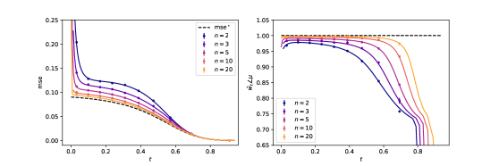
Figure 4: $\sigma=0.3,\lambda=0.1,\alpha(t)=\cos(\nicefrac{{\pi t}}{{2}}),\beta(t)=\sin(\nicefrac{{\pi t}}{{2}})$. Solid lines: theoretical predictions for the MSE of Result A.1 (left) and the cosine similarity of Result A.2 (right). Different colors correspond to different number of samples $n$. Dots: numerical simulations, corresponding to training the DAE (9) on the risk (10) using the Pytorch implementation of full-batch Adam, with learning rate $0.01$ over $2000$ epochs and weight decay $\lambda=0.1$. The experimental points correspond to a single instance of the model, and were collected in dimension $d=500$. In the left plot, the dashed line represent the oracle baseline (53).

Appendix B Derivation of Result III.1

In this Appendix, we detail the heuristic derivation of Result III.1. Given an initial condition $X_{0}\sim\rho_{0}$, a sample follows the transport (7)

$$\frac{d}{dt}X_{t}=\left(\dot{\beta}(t)\hat{c}_{t}+\frac{\dot{\alpha}(t)}{\alpha(t)}(1-\hat{c}_{t}\beta(t))\right)X_{t}+\left(\dot{\beta}(t)-\frac{\dot{\alpha}(t)}{\alpha(t)}\beta(t)\right)\hat{w}_{t}\mathrm{sign}(\hat{w}_{t}^{\top}X_{t})$$ (57)

driven by the learnt velocity field $\hat{b}$ (6). This follows from Result II.1 and (7). Taking scalar products with $\mu,\xi,\eta$,

$$\begin{cases}\frac{d}{dt}\frac{X_{t}^{\top}\mu}{d}=\left(\dot{\beta}(t)\hat{c}_{t}+\frac{\dot{\alpha}(t)}{\alpha(t)}(1-\hat{c}_{t}\beta(t))\right)\frac{X_{t}^{\top}\mu}{d}+\left(\dot{\beta}(t)-\frac{\dot{\alpha}(t)}{\alpha(t)}\beta(t)\right)\mathrm{sign}(\hat{w}_{t}^{\top}X_{t})\frac{\hat{w}_{t}^{\top}\mu}{d}\\ \frac{d}{dt}\frac{X_{t}^{\top}\xi}{nd}=\left(\dot{\beta}(t)\hat{c}_{t}+\frac{\dot{\alpha}(t)}{\alpha(t)}(1-\hat{c}_{t}\beta(t))\right)\frac{X_{t}^{\top}\xi}{nd}+\left(\dot{\beta}(t)-\frac{\dot{\alpha}(t)}{\alpha(t)}\beta(t)\right)\mathrm{sign}(\hat{w}_{t}^{\top}X_{t})\frac{\hat{w}_{t}^{\top}\xi}{nd}\\ \frac{d}{dt}\frac{X_{t}^{\top}\eta}{nd\sigma^{2}}=\left(\dot{\beta}(t)\hat{c}_{t}+\frac{\dot{\alpha}(t)}{\alpha(t)}(1-\hat{c}_{t}\beta(t))\right)\frac{X_{t}^{\top}\eta}{nd\sigma^{2}}+\left(\dot{\beta}(t)-\frac{\dot{\alpha}(t)}{\alpha(t)}\beta(t)\right)\mathrm{sign}(\hat{w}_{t}^{\top}X_{t})\frac{\hat{w}_{t}^{\top}\eta}{nd\sigma^{2}}\end{cases}.$$ (58)

It is reasonable to assume the sign $\mathrm{sign}(\hat{w}_{t}^{\top}X_{t})$ stays constant during the transport, and therefore takes value $\pm 1$ with equal probability $\nicefrac{{1}}{{2}}$, according to the initial condition $X_{0}$. This is an heuristic assumption which is further confirmed numerically. Finally, plugging the definitions (16) and (13) in (58), one reaches

$$\begin{cases}\frac{d}{dt}M_{t}=\left(\dot{\beta}(t)\hat{c}_{t}+\frac{\dot{\alpha}(t)}{\alpha(t)}(1-\hat{c}_{t}\beta(t))\right)M_{t}+\left(\dot{\beta}(t)-\frac{\dot{\alpha}(t)}{\alpha(t)}\beta(t)\right)m_{t}\\ \frac{d}{dt}Q^{\xi}_{t}=\left(\dot{\beta}(t)\hat{c}_{t}+\frac{\dot{\alpha}(t)}{\alpha(t)}(1-\hat{c}_{t}\beta(t))\right)Q^{\xi}_{t}+\left(\dot{\beta}(t)-\frac{\dot{\alpha}(t)}{\alpha(t)}\beta(t)\right)q^{\xi}_{t}\\ \frac{d}{dt}Q^{\eta}_{t}=\left(\dot{\beta}(t)\hat{c}_{t}+\frac{\dot{\alpha}(t)}{\alpha(t)}(1-\hat{c}_{t}\beta(t))\right)Q^{\eta}_{t}+\left(\dot{\beta}(t)-\frac{\dot{\alpha}(t)}{\alpha(t)}\beta(t)\right)q^{\eta}_{t}\end{cases},$$ (59)

which recovers equation (15) of Result III.1. Noting that $\hat{w}_{t}\in\mathrm{span}(\mu,\xi,\eta)$ (see Result II.1), the differential equation (57) becomes, for the orthogonal component $X_{t}^{\perp}\in\mathrm{span}(\mu,\xi,\eta)^{\perp}$

$$\frac{d}{dt}X_{t}^{\perp}=\left(\dot{\beta}(t)\hat{c}_{t}+\frac{\dot{\alpha}(t)}{\alpha(t)}(1-\hat{c}_{t}\beta(t))\right)X_{t}^{\perp}$$ (60)

which recovers (17) of Result III.1. This can be explicitly solved as

$$X_{t}^{\perp}=X_{0}^{\perp}e^{\int\limits_{0}^{t}\left(\dot{\beta}(t)\hat{c}_{t}+\frac{\dot{\alpha}(t)}{\alpha(t)}(1-\hat{c}_{t}\beta(t))\right)dt}$$ (61)

Finally,

$$Q_{t} \equiv\lVert X_{t}\lVert^{2}$$

$$=M_{t}^{2}+n(Q_{t}^{\xi})^{2}+n\sigma^{2}(Q^{\eta}_{t})^{2}+\lVert X_{t}^{\perp}\lVert^{2}$$

$$=M_{t}^{2}+n(Q_{t}^{\xi})^{2}+n\sigma^{2}(Q^{\eta}_{t})^{2}+e^{2\int\limits_{0}^{t}\left(\dot{\beta}(t)\hat{c}_{t}+\frac{\dot{\alpha}(t)}{\alpha(t)}(1-\hat{c}_{t}\beta(t))\right)dt}$$ (62)

which concludes the derivation of Result III.1 ∎

B.1 Derivation of Remark III.2

The derivation of Remark III.2 follows identical steps, building on the observation that the discretized flow 19 is explicitly expressed as

$$X_{t_{k+1}}=X_{t_{k}} +\delta t_{k}\left(\dot{\beta}(t_{k})\hat{c}_{t_{k}}+\frac{\dot{\alpha}(t_{k})}{\alpha(t_{k})}(1-\hat{c}_{t_{k}}\beta(t_{k}))\right)X_{t_{k}}$$

$$+\delta t_{k}\left(\dot{\beta}(t_{k})-\frac{\dot{\alpha}(t_{k})}{\alpha(t_{k})}\beta(t_{k})\right)\hat{w}_{t_{k}}\mathrm{sign}(\hat{w}_{t_{k}}^{\top}X_{t_{k}})$$ (63)

Taking overlaps with $\mu,\xi,\eta$ yields

$$\begin{cases}\frac{\mu^{\top}X_{t_{k+1}}}{d}={\scriptstyle\frac{\mu^{\top}X_{t_{k}}}{d}+\delta t_{k}\left(\dot{\beta}(t_{k})\hat{c}_{t_{k}}+\frac{\dot{\alpha}(t_{k})}{\alpha(t_{k})}(1-\hat{c}_{t_{k}}\beta(t_{k}))\right)\frac{\mu^{\top}X_{t_{k}}}{d}+\delta t_{k}\left(\dot{\beta}(t_{k})-\frac{\dot{\alpha}(t_{k})}{\alpha(t_{k})}\beta(t_{k})\right)\mathrm{sign}(\hat{w}_{t_{k}}^{\top}X_{t_{k}})}\frac{\mu^{\top}\hat{w}_{t_{k}}}{d}\\ \frac{\xi^{\top}X_{t_{k+1}}}{nd}={\scriptstyle\frac{\xi^{\top}X_{t_{k}}}{nd}+\delta t_{k}\left(\dot{\beta}(t_{k})\hat{c}_{t_{k}}+\frac{\dot{\alpha}(t_{k})}{\alpha(t_{k})}(1-\hat{c}_{t_{k}}\beta(t_{k}))\right)\frac{\xi^{\top}X_{t_{k}}}{nd}+\delta t_{k}\left(\dot{\beta}(t_{k})-\frac{\dot{\alpha}(t_{k})}{\alpha(t_{k})}\beta(t_{k})\right)\mathrm{sign}(\hat{w}_{t_{k}}^{\top}X_{t_{k}})}\frac{\xi^{\top}\hat{w}_{t_{k}}}{nd}\\ \frac{\eta^{\top}X_{t_{k+1}}}{nd\sigma^{2}}={\scriptstyle\frac{\eta^{\top}X_{t_{k}}}{nd\sigma^{2}}+\delta t_{k}\left(\dot{\beta}(t_{k})\hat{c}_{t_{k}}+\frac{\dot{\alpha}(t_{k})}{\alpha(t_{k})}(1-\hat{c}_{t_{k}}\beta(t_{k}))\right)\frac{\eta^{\top}X_{t_{k}}}{nd\sigma^{2}}+\delta t_{k}\left(\dot{\beta}(t_{k})-\frac{\dot{\alpha}(t_{k})}{\alpha(t_{k})}\beta(t_{k})\right)\mathrm{sign}(\hat{w}_{t_{k}}^{\top}X_{t_{k}})}\frac{\eta^{\top}\hat{w}_{t_{k}}}{nd\sigma^{2}}\end{cases}$$ (64)

Like in the continuous case, one makes the heuristic assumption that $\mathrm{sign}(\hat{w}_{t_{k}}^{\top}X_{t_{k}})$ stays constant along the flow, taking value $\pm 1$ with equal probability, depending on the initial condition. Doing so yields

$$\begin{cases}M_{t_{k+1}}=M_{t_{k}}+\delta t_{k}\left(\dot{\beta}(t_{k})\hat{c}_{t_{k}}+\frac{\dot{\alpha}(t_{k})}{\alpha(t_{k})}(1-\hat{c}_{t_{k}}\beta(t_{k}))\right)M_{t_{k}}+\delta t_{k}\left(\dot{\beta}(t_{k})-\frac{\dot{\alpha}(t_{k})}{\alpha(t_{k})}\beta(t_{k})\right)m_{t_{k}}\\ Q^{\xi}_{t_{k+1}}=Q^{\xi}_{t_{k}}+\delta t_{k}\left(\dot{\beta}(t_{k})\hat{c}_{t_{k}}+\frac{\dot{\alpha}(t_{k})}{\alpha(t_{k})}(1-\hat{c}_{t_{k}}\beta(t_{k}))\right)Q^{\xi}_{t_{k}}+\delta t_{k}\left(\dot{\beta}(t_{k})-\frac{\dot{\alpha}(t_{k})}{\alpha(t_{k})}\beta(t_{k})\right)q^{\xi}_{t_{k}}\\ Q^{\eta}_{t_{k+1}}=Q^{\eta}_{t_{k}}+\delta t_{k}\left(\dot{\beta}(t_{k})\hat{c}_{t_{k}}+\frac{\dot{\alpha}(t_{k})}{\alpha(t_{k})}(1-\hat{c}_{t_{k}}\beta(t_{k}))\right)Q^{\eta}_{t_{k}}+\delta t_{k}\left(\dot{\beta}(t_{k})-\frac{\dot{\alpha}(t_{k})}{\alpha(t_{k})}\beta(t_{k})\right)q^{\eta}_{t_{k}}\end{cases},$$ (65)

which recovers (20). Equation (21) follows from (B.1) and the fact that $\hat{w}_{t}\in\mathrm{span}(\mu,\xi,\eta)$, see Result II.1. This recursion can be explicitly solved as

$$X^{\perp}_{t_{k+1}}=X_{t_{0}}^{\perp}\prod\limits_{\ell=0}^{k}\left(\scriptstyle 1+\left(\dot{\beta}(t_{\ell})+\frac{\dot{\alpha}(t_{\ell})}{\alpha(t_{\ell})}(1-\hat{c}_{t_{\ell}}\beta(t_{\ell}))\right)\delta t_{\ell}\right)^{2}.$$ (66)

Using the fact that $\lVert X_{t_{0}}^{\perp}\lVert/d=1$ with high probability and the definition of the summary statistics $Q$ finally yields (22).∎

B.2 Derivation of Corollary III.3

As implied by Result III.1, the mean of the generated mixture is contained in $\mathrm{span}(\mu,\xi,\eta)$ and characterized by the summary statistics $M_{1},Q^{\eta}_{1},Q^{\xi}_{1}$ at time $t=1$. Furthermore

$$\frac{1}{d}\lVert\hat{\mu}-\mu\lVert^{2} =\frac{1}{d}\lVert\hat{\mu}\lVert^{2}-2\frac{\hat{\mu}^{\top}\mu}{d}+1$$

$$=M_{1}^{2}+n(Q_{1}^{\xi})^{2}+n\sigma^{2}(Q^{\eta}_{1})^{2}-2R_{1}+1.$$ (67)

This recovers (23). Equation (24) follows from the definition of the cosine similarity.

The derivation of the $\Theta_{n}(\nicefrac{{1}}{{n}})$ decay of this distance require more work. The first step lies in the analysis of the exact flow (1).

Remark B.1.

(exact velocity field) For the target density $\rho_{1}$ (8), $b$ is given by [14, 1] as

$$b(x,t)=\left(\dot{\beta}(t)-\frac{\dot{\alpha}(t)}{\alpha(t)}\beta(t)\right)\left(\frac{\beta(t)\sigma^{2}}{\alpha(t)^{2}+\beta(t)^{2}\sigma^{2}}x+\frac{\alpha(t)^{2}}{\alpha(t)^{2}+\beta(t)^{2}\sigma^{2}}\mu\times\tanh(\mu^{\top}x)\right)+\frac{\dot{\alpha}(t)}{\alpha(t)}x.$$ (68)

The formula (68) follows from an application of Tweedie’s formula [14] for the the density (8). Note that with high probability for $x\sim\rho_{0}$, or for any $x$ such that $\mu^{\top}x\gg 1$,

$$\tanh(\mu^{\top}x)=\mathrm{sign}(\mu^{\top}x)+o_{d}(1).$$ (69)

One is now in a position to characterize the exact flow (1).

Corollary B.2.

(Summary statistics for the exact flow) Let $X^{\star}_{t}$ be a solution of the exact flow (1) from an initialization $X^{\star}_{0}\sim\rho_{0}$. Consider the summary statistic

$$M^{\star}_{t}\equiv\frac{\mu^{\top}X_{t}^{\star}}{d}.$$ (70)

Asymptotically, $M^{\star}_{t}$ is equal with probability $\nicefrac{{1}}{{2}}$ to the solution of the differential equation

$$\frac{d}{dt}M^{\star}_{t}=\left(\dot{\beta}(t)c_{t}+\frac{\dot{\alpha}(t)}{\alpha(t)}(1-c_{t}\beta(t))\right)M^{\star}_{t}+\left(\dot{\beta}(t)-\frac{\dot{\alpha}(t)}{\alpha(t)}\beta(t)\right)\frac{\alpha(t)^{2}}{\alpha(t)^{2}+\beta(t)^{2}\sigma^{2}}$$ (71)

and with probability $\nicefrac{{1}}{{2}}$ to the opposite thereof. We have introduced

$$c_{t}\equiv\frac{\beta(t)\sigma^{2}}{\alpha(t)^{2}+\beta(t)^{2}\sigma^{2}}.$$ (72)

Corollary B.2 follows from (68) using a derivation identical to that of Result III.1, presented in Appendix B, provided the heuristic assumption is made that the tanh can always be approximated by a sign (69) along the flow. To show that the learnt flow III.1 converges to the exact flow, observe the following scalings:

Remark B.3.

Let $t>0$ and $m_{t},q^{\xi}_{t},q^{\eta}_{t}$ be defined by result II.1. Then

$$\left|m_{t}-\frac{\alpha(t)^{2}}{\alpha(t)^{2}+\beta(t)^{2}\sigma^{2}}\right|=\Theta_{n}(\nicefrac{{1}}{{n}}), \left|\hat{c}_{t}-c_{t}\right|=\Theta_{n}(\nicefrac{{1}}{{n}}), q^{\xi}_{t}=\Theta_{n}(\nicefrac{{1}}{{n}}), q^{\eta}_{t}=\Theta_{n}(\nicefrac{{1}}{{n}}).$$ (73)

These observations immediately imply the following asymptotics, characterizing the difference between the learnt flow (7) and the exact flow (1):

Corollary B.4.

(Convergence of the learnt flow) Let $X^{\star}_{t}$ (resp. $X_{t}$) be a solution of the exact flow (1) (resp. learnt flow (7)), from a common initialization $X_{0}\sim\rho_{0}$. Define the following summary statistics:

$$\epsilon^{m}_{t}\equiv\frac{1}{d}\mu^{\top}(X_{t}-X^{\star}_{t}), \epsilon^{\xi}_{t}\equiv\frac{1}{nd}\xi^{\top}(X_{t}-X^{\star}_{t}), \epsilon^{\eta}_{t}\equiv\frac{1}{nd\sigma^{2}}\eta^{\top}(X_{t}-X^{\star}_{t})$$ (74)

Then with high probability these statistics obey the differential equations

$$\begin{cases}\frac{d}{dt}\epsilon^{m}_{t}=\left(\dot{\beta}(t)c_{t}+\frac{\dot{\alpha}(t)}{\alpha(t)}(1-c_{t}\beta(t))\right)\epsilon^{m}_{t}+\Theta_{n}(\nicefrac{{1}}{{n}})\\ \frac{d}{dt}\epsilon^{\xi}_{t}=\left(\dot{\beta}(t)c_{t}+\frac{\dot{\alpha}(t)}{\alpha(t)}(1-c_{t}\beta(t))\right)\epsilon^{\xi}_{t}+\Theta_{n}(\nicefrac{{1}}{{n}})\\ \frac{d}{dt}\epsilon^{\eta}_{t}=\left(\dot{\beta}(t)c_{t}+\frac{\dot{\alpha}(t)}{\alpha(t)}(1-c_{t}\beta(t))\right)\epsilon^{\eta}_{t}+\Theta_{n}(\nicefrac{{1}}{{n}})\end{cases},$$ (75)

from the initial condition $\epsilon^{m,\xi,\eta}_{0}=0$. Therefore at time $t=1$

$$\epsilon_{1}^{m}=\Theta_{n}(\nicefrac{{1}}{{n}}), \epsilon_{1}^{\xi}=\Theta_{n}(\nicefrac{{1}}{{n}}), \epsilon_{1}^{\eta}=\Theta_{n}(\nicefrac{{1}}{{n}}).$$ (76)

Corollary B.4 follows from substracting the differential equations governing the learnt flow of Result III.1 and the true flow of Corollary B.2, using the scaling derived in Remark B.3. Finally, noting that $M^{\star}_{1}=1$ by definition of the exact flow,

$$\frac{1}{d}\lVert\hat{\mu}-\mu\lVert^{2} =\frac{1}{d}\lVert\epsilon_{1}^{m}\mu+\epsilon_{1}^{\xi}\xi+\epsilon_{1}^{\eta}\eta\lVert^{2}$$

$$=(\epsilon_{1}^{m})^{2}+n(\epsilon_{1}^{\xi})^{2}+n\sigma^{2}(\epsilon_{1}^{\eta})^{2}+O_{d}(\nicefrac{{1}}{{\sqrt{d}}})$$

$$=\Theta_{n}(\nicefrac{{1}}{{n}}).$$ (77)

In the last line, we used Corollary B.4. This concludes the derivation of Corollary III.3. Fig. 2 (right) gives a PCA visualization of the convergence of the generated density $\hat{\rho}_{1}$ to the target density $\rho_{1}$ as the number available training samples $n$ accrues.∎

Appendix C Derivation of Remark IV.1

In this appendix, we analyze the performance of the Bayes-optimal estimator of the cluster mean, defined as the estimator minimizing the average MSE knowing the train set $\mathcal{D}=\{x_{0}^{\mu},x_{1}^{\mu}\}_{\mu=1}^{n}$, the clusters variance $\sigma$, but not the mean $\mu$. This estimator yields the information-theoretically minimal achievable MSE, and is known to be given by the mean of the posterior distribution over the estimate $w$ of the true mean $\mu$ :

$$\mathbb{P}(w|\mathcal{D},\sigma) =e^{-\frac{1}{2}\lVert w\lVert^{2}}\prod\limits_{\mu=1}^{n}\left[\frac{1}{2}e^{-\frac{1}{2\sigma^{2}}\lVert x_{1}^{\mu}-w\lVert^{2}}+\frac{1}{2}e^{-\frac{1}{2\sigma^{2}}\lVert x_{1}^{\mu}+w\lVert^{2}}\right]$$

$$\equiv\frac{1}{Z}e^{-\frac{1}{2\hat{\sigma}^{2}}\lVert w\lVert^{2}+\sum\limits_{\mu=1}^{n}\ln\cosh\left(\frac{w^{\top}x_{1}^{\mu}}{\sigma^{2}}\right)},$$ (78)

where

$$\hat{\sigma}^{2}\equiv\frac{\sigma^{2}}{n+\sigma^{2}}.$$ (79)

We remind the reader that the prior distribution over the cluster mean is supposed to be the standard Gaussian prior $\mathcal{N}(0,\mathbb{I}_{d})$. In high dimensions, statistics associated to the posterior distribution (C) are expected to concentrate. Again, it is useful to study the partition function (normalization) $Z$ to access some key summary statistics. The partition function reads

$$Z =\int dwe^{-\frac{1}{2\hat{\sigma}^{2}}\lVert w\lVert^{2}+\sum\limits_{\mu=1}^{n}\ln\cosh\left(\frac{w^{\top}x_{1}^{\mu}}{\sigma^{2}}\right)}$$

$$=\int dqd\hat{q}dmd\hat{m}\prod\limits_{\mu=1}^{n}dq_{\eta}^{\mu}d\hat{q}_{\eta}^{\mu}e^{\frac{d}{2}q\hat{q}+d\sum\limits_{\mu=1}^{n}q_{\eta}^{\mu}\hat{q}_{\eta}^{\mu}+dm\hat{m}}$$

$$~{}~{}~{}~{}\int dwe^{-\frac{\hat{q}}{2}\lVert w\lVert^{2}-\frac{1}{2\hat{\sigma}^{2}}\lVert w\lVert^{2}-\left(\hat{m}\mu+\sum\limits_{\mu=1}^{n}\hat{q}_{\eta}^{\mu}s^{\mu}z^{\mu}\right)^{\top}w}e^{-d\sum\limits_{\mu=1}^{n}\ln\cosh^{\nicefrac{{1}}{{d}}}\left[\frac{d}{\sigma^{2}}\left(m+q_{\eta}^{\mu}\right)\right]}$$ (80)

As in Appendix A, we have introduced the summary statistics

$$q_{\eta}^{\mu}\equiv s^{\mu}\frac{w^{\top}z^{\mu}}{d}, m=\frac{w^{\top}\mu}{d}.$$ (81)

The integral of (C) can be evaluated using a Laplace approximation. Again, we assume the extremizer is realized at the sample-symmetric point

$$\forall 1\leq\mu\leq n,~{}q^{\mu}_{\eta}=q_{\eta},$$

$$\forall 1\leq\mu\leq n,~{}\hat{q}^{\mu}_{\eta}=\hat{q}_{\eta}.$$ (82)

The partition function (C) then reduces to

$$Z =\int dqd\hat{q}dq_{\eta}d\hat{q}_{\eta}dmd\hat{m}e^{\frac{d}{2}q\hat{q}+dnq_{\eta}\hat{q}_{\eta}+dm\hat{m}}$$

$$~{}~{}~{}~{}\int dwe^{-\frac{\hat{q}}{2}\lVert w\lVert^{2}-\frac{1}{2\hat{\sigma}^{2}}\lVert w\lVert^{2}-\left(\hat{m}\mu+\hat{q}_{\eta}\eta\right)^{\top}w}e^{-d\sum\limits_{\mu=1}^{n}\ln\cosh^{\nicefrac{{1}}{{d}}}\left[\frac{d}{\sigma^{2}}\left(m+q_{\eta}\right)\right]}$$

$$=\int dqd\hat{q}dq_{\eta}d\hat{q}_{\eta}dmd\hat{m}e^{\frac{d}{2}q\hat{q}+dnq_{\eta}\hat{q}_{\eta}+dm\hat{m}}e^{-d\sum\limits_{\mu=1}^{n}\ln\cosh^{\nicefrac{{1}}{{d}}}\left[\frac{d}{\sigma^{2}}\left(m+q_{\eta}\right)\right]}$$

$$~{}~{}~{}~{}\frac{1}{(1+\hat{\sigma}^{2}\hat{q})^{\nicefrac{{d}}{{2}}}}e^{\frac{d}{2}\frac{\hat{\sigma}^{2}}{1+\hat{\sigma}^{2}\hat{q}}(\hat{m}^{2}+n\sigma^{2}\hat{q}_{\eta}^{2})}.$$ (83)

Therefore $\hat{q}_{\eta},q_{\eta},\hat{m},m$ must extremize the effective action

$$\Phi=\frac{q\hat{q}}{2}+nq_{\eta}\hat{q}_{\eta}+m\hat{m}-\frac{1}{2}\ln(1+\hat{\sigma}^{2}\hat{q})+\frac{\hat{\sigma}^{2}}{2(1+\hat{\sigma}^{2}\hat{q})}\left(\hat{m}^{2}+n\sigma^{2}\hat{q}_{\eta}^{2}\right)+\frac{n}{\sigma^{2}}|m+q_{\eta}|,$$ (84)

leading to

$$\begin{cases}\hat{q}_{\eta}=-\frac{1}{\sigma^{2}}\\ \hat{m}=-\frac{n}{\sigma^{2}}\end{cases}, \begin{cases}q_{\eta}=-\hat{q}_{\eta}\sigma^{2}\hat{\sigma}^{2}=\frac{\sigma^{2}}{n+\sigma^{2}}\\ m=-\hat{m}\hat{\sigma}^{2}=\frac{n}{n+\sigma^{2}}\end{cases}.$$ (85)

Refining $\sigma^{2}q_{\eta}\leftarrow q_{\eta}$ so that

$$q_{\eta}\equiv\frac{w^{\top}\eta}{nd\sigma^{2}},$$ (86)

as in Remark IV.1, one finally reaches

$$q_{\eta}=\frac{1}{n+\sigma^{2}}, m=\frac{n}{n+\sigma^{2}},$$ (87)

Thus, remembering $\hat{\mu}^{\star}(\mathcal{D})=\langle w\rangle$ (where the bracket notation denotes averages with respect to the posterior $P(\cdot|\mathcal{D},\sigma)$:

$$\frac{\mu^{\top}\hat{\mu}^{\star}(\mathcal{D})}{d}=\left\langle\frac{w^{\top}\mu}{d}\right\rangle=\frac{n}{n+\sigma^{2}}, \frac{\eta^{\top}\hat{\mu}^{\star}(\mathcal{D})}{nd\sigma^{2}}=\left\langle\frac{w^{\top}\eta}{nd\sigma^{2}}\right\rangle=\frac{1}{n+\sigma^{2}},$$ (88)

using the concentration of the bracketed quantities. Furthermore,

$$\frac{\lVert\hat{\mu}^{\star}(\mathcal{D})\lVert^{2}}{d}=\frac{1}{d}\lVert\langle w\rangle\lVert^{2}=\frac{\mu^{\top}\langle w\rangle}{d}=m.$$ (89)

We employed the Nishimori identity [26, 17].Note further the identity:

$$\frac{\lVert\hat{\mu}^{\star}(\mathcal{D})\lVert^{2}}{d}=m=m^{2}+n\sigma^{2}q_{\eta}^{2}=\frac{1}{d}\lVert m\mu+q_{\eta}\eta\lVert^{2},$$ (90)

which implies that the norm of $\hat{\mu}^{\star}(\mathcal{D})$ is equal to the norm of its projection in $\mathrm{span}(\mu,\eta)$, which means that asymptotically the former is contained in the latter. One is now in a position to derive the Bayes-optimal MSE of Remark IV.1. With high probability

$$\frac{1}{d}\lVert\hat{\mu}^{\star}(\mathcal{D})-\mu\lVert^{2}=m+1-2m=1-m=\frac{\sigma^{2}}{n+\sigma^{2}}.$$ (91)

This completes the derivation of Remark IV.1 ∎

Appendix D Further settings

D.1 Imbalanced clusters

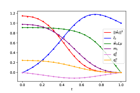
Figure 5: $n=4,\sigma=0.9,\lambda=0.1,\alpha(t)=1-t,\beta(t)=t$. Imbalanced mixture with relative weights $\rho=0.24$ and $1-\rho=0.76$. Solid lines: theoretical predictions of Result II.1: squared norm of the DAE weight vector $\lVert\hat{\bm{w}}_{t}\lVert^{2}$ (red), skip connection strength $\hat{c}_{t}$ (blue) cosine similarity between the weight vector $\hat{\bm{w}}_{t}$ and the target cluster mean $\bm{\mu}$, $\hat{\bm{w}}_{t}\angle\bm{\mu}\equiv\hat{\bm{w}}_{t}^{\top}\bm{\mu}/\lVert\bm{\mu}\lVert\lVert\hat{\bm{w}}_{t}\lVert$ (green), components $m_{t},q^{\xi}_{t},q^{\eta}_{t}$ of $\hat{\bm{w}}_{t}$ along the vectors $\bm{\mu},\bm{\xi},\bm{\eta}$ (purple, pink, orange). Dots: numerical simulations in $d=5\times 10^{4}$, corresponding to training the DAE (9) on the risk (10) uisng the Pytorch implementation of full-batch Adam, with learning rate $0.001$ over $20000$ epochs and weight decay $\lambda=0.1$. The experimental points correspond to a single instance of the model.

In this appendix, we address the case of a binary homoscedastic but imbalanced mixture

$$\rho_{1}=\rho\mathcal{N}(\mu,\sigma^{2}\mathbb{I}_{d})+(1-\rho)\mathcal{N}(-\mu,\sigma^{2}\mathbb{I}_{d}),$$ (92)

where $\rho\in(0,1)$ controls the relative weights of the two clusters. The target density considered in the main text (8) thus corresponds to the special case $\rho=\nicefrac{{1}}{{2}}$.

It is immediate to verify that the derivations presented in Appendices A, B carry through. In other words, Result II.1, Result III.1 and Corollary III.3 still exactly hold. Figure 5 shows that the sharp characterization of Result II.1 indeed still tightly captures the learning curves of a DAE, trained on imbalanced clusters, using the Pytorch [28] implementation of the Adam [19] optimizer.

An important consequence of this observation is that the generative model will generate a balanced density $\hat{\rho}_{1}$, failing to capture the asymmetry of the target distribution $\rho_{1}$. This echoes the findings of [4] in the related setting of a target ferromagnetic Curie-Weiss model, where they argue that the asymmetry of the ground state can only be learnt for $n\gg d$ samples.

D.2 DAE without skip connection

In this appendix, we examine the importance of the skip connection in the DAE architecture (9). More precisely, we consider the generative model parameterized by the DAE without skip connection

$$g_{w_{t}}(x)=w_{t}\varphi(w_{t}^{\top}x)$$ (93)

where $\varphi$ is an activation admitting horizontal asymptots at $+1$ ($-1$) in $+\infty$ ($-\infty$). A tight characterization of the learnt weight $\hat{w}_{t}$ can also straightfowardly be accessed, and is summarized in the following result, which is the equivalent of Result II.1 for the DAE without skip connection (93)

Result D.1.

(Sharp characterization of the trained weight of (93)) For any given activation $\varphi$ satisfying $\varphi(x)\xrightarrow[]{x\to\pm\infty}\pm 1$ and any $t\in[0,1]$, in the limit $d\to\infty$, $n,\nicefrac{{\lVert\bm{\mu}\lVert^{2}}}{{d}},\sigma=\Theta_{d}(1)$, the learnt weight vector $\hat{\bm{w}}_{t}$ of the DAE without skip connection (93) trained on the loss (10) is asymptotically contained in $\mathrm{span}(\bm{\mu},\bm{\eta})$ (in the sense that its projection on the orthogonal space $\mathrm{span}(\bm{\mu},\bm{\eta})^{\perp}$ has asymptotically vanishing norm). The components of $\hat{\bm{w}}_{t}$ along each of these two vectors is given by the summary statistics

$$m_{t}=\frac{\bm{\mu}^{\top}\hat{\bm{w}}_{t}}{d}, q^{\eta}_{t}=\frac{\hat{\bm{w}}_{t}^{\top}\bm{\eta}}{nd\sigma^{2}},$$ (94)

which concentrate as $d\to\infty$ to the time-constant quantities characterized by the closed-form formulae

$$m=\frac{n}{\lambda+n}, q^{\eta}=\frac{1}{\lambda+n}.$$ (95)

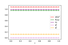
Figure 6: $n=4,\sigma=0.9,\lambda=0.1,\alpha(t)=1-t,\beta(t)=t$. Solid lines: theoretical predictions of Result II.1: squared norm of the weight vector $\lVert\hat{\bm{w}}_{t}\lVert^{2}$ of the DAE without skip connection (93) (red), skip connection strength $\hat{c}_{t}$ (blue) cosine similarity between the weight vector $\hat{\bm{w}}_{t}$ and the target cluster mean $\bm{\mu}$, $\hat{\bm{w}}_{t}\angle\bm{\mu}\equiv\hat{\bm{w}}_{t}^{\top}\bm{\mu}/\lVert\bm{\mu}\lVert\lVert\hat{\bm{w}}_{t}\lVert$ (green), components $m_{t},q^{\xi}_{t},q^{\eta}_{t}$ of $\hat{\bm{w}}_{t}$ along the vectors $\bm{\mu},\bm{\xi},\bm{\eta}$ (purple, pink, orange). Dots: numerical simulations in $d=5\times 10^{4}$, corresponding to training the DAE without skip connection (93) on the risk (10) uisng the Pytorch implementation of full-batch Adam, with learning rate $0.001$ over $20000$ epochs and weight decay $\lambda=0.1$. The experimental points correspond to a single instance of the model.

Result D.1 follows from a straightforward adapatation of the derivation of Result II.1 as presented in Appendix A. In fact, it naturally corresponds to setting the skip connection strength $c$ to $0$ in the expression of the log partition function (A.2). (94) corresponds to the zero-gradient condition thereof.

A striking consequence of Result D.1 is that asymptotically the trained vector $\hat{w}$ of the DAE (93) does not depend on the time $t$. Fig. 6 provides further support of this fact, as the summary statistics measured in simulations – training the DAE (93) using the Pytorch implementation of full-batch Adam – are also observed to be constant in time, and furthermore to agree well with the theoretical prediction. As for the analysis presented in the main text, it is possible to track the generative flow with a finite set of summary statistics. This is the object of the following result:

Result D.2.

(Summary statistics for the no-skip connection case) Le $\bm{X}_{t}$ be a solution of the ordinary differential equation (7) with initial condition $\bm{X}_{0}$, when parametrized by the DAE without skip connection (93). For a given $t$, the projection of $\bm{X}_{t}$ on $\mathrm{span}(\bm{\mu},,\bm{\eta})$ is characterized by the summary statistics

$$M_{t}\equiv\frac{\bm{X}_{t}^{\top}\bm{\mu}}{d}, Q^{\eta}_{t}\equiv\frac{\bm{X}_{t}^{\top}\bm{\eta}}{nd\sigma^{2}}.$$ (96)

With probability asymptotically $\nicefrac{{1}}{{2}}$ the summary statistics $M_{t},Q^{\eta}_{t}$ (15) concentrate for all $t$ to the solution of the ordinary differential equations

$$\begin{cases}\frac{d}{dt}M_{t}=\frac{\dot{\alpha}(t)}{\alpha(t)}M_{t}+\left(\dot{\beta}(t)-\frac{\dot{\alpha}(t)}{\alpha(t)}\beta(t)\right)\frac{n}{\lambda+n}\\ \frac{d}{dt}Q^{\eta}_{t}=\frac{\dot{\alpha}(t)}{\alpha(t)}Q^{\eta}_{t}+\left(\dot{\beta}(t)-\frac{\dot{\alpha}(t)}{\alpha(t)}\beta(t)\right)\frac{1}{\lambda+n}\end{cases}.$$ (97)

The derivation of Result D.2 can be made along the exact same lines as the one for Result III.1, presented in Appendix B. An important observation is that the flows (97) are actually the exact flows corresponding to a particular Gaussian mixture, as explicited in the following remark:

Remark D.3.

(Generated density) The summary statistics evolution (97) are the same evolutions that would follow from the velocity field

$$b(x,t)=\left(\dot{\beta}(t)-\frac{\dot{\alpha}(t)}{\alpha(t)}\beta(t)\right)\left(\hat{\mu}\times\tanh(\hat{\mu}^{\top}x)\right)+\frac{\dot{\alpha}(t)}{\alpha(t)}x.$$ (98)

where

$$\hat{\mu}\equiv\frac{n}{\lambda+n}\mu+\frac{1}{\lambda+n}\eta.$$ (99)

Comparing with (68), this is the exact velocity field associated to the singular Gaussian mixture

$$\hat{\rho}_{1}(x)=\frac{1}{2}\delta(x-\hat{\mu})+\frac{1}{2}\delta(x+\hat{\mu}).$$ (100)

The generative model parameterized by the DAE without skip connection (93) thus learns a singular density, which is a sum of two Dirac atoms, centered at $\pm\hat{\mu}$. It thus fails to generate a good approximation of the target $\rho_{1}$ (8). Note however that interestingly $\hat{\mu}$ remains a good approximation of the true mean $\mu$, and actually converges thereto as $n\to\infty$. This is made more precise by the following result:

Remark D.4.

(mse in the no-skip-connection case) Let $\hat{\mu}$ be the cluster mean of the estimated density $\hat{\rho}_{1}$, as defined in Remark D.3. Then its squared distance to the true mean $\mu$ is

$$\frac{1}{d}\lVert\hat{\mu}-\mu\lVert^{2}=\frac{\lambda^{2}+n\sigma^{2}}{(\lambda+n)^{2}}$$ (101)

The minimum is achieved for $\lambda=\sigma^{2}$ and is equal to the Bayes MSE IV.1. In particular, this MSE decays as $\Theta_{n}(\nicefrac{{1}}{{n}})$.

Strikingly, the generative model parametrized by (93) manages to achieve the Bayes optimal $\Theta_{n}(\nicefrac{{1}}{{n}})$ rate in terms of the estimation MSE over the cluster means, but completely fails to accurately estimate the true variance.

References

- [1] M. S. Albergo, Nicholas M. Boffi, and Eric Vanden-Eijnden. Stochastic interpolants: A unifying framework for flows and diffusions. ArXiv, abs/2303.08797, 2023.
- [2] Michael S Albergo and Eric Vanden-Eijnden. Building normalizing flows with stochastic interpolants. arXiv preprint arXiv:2209.15571, 2022.
- [3] Joe Benton, George Deligiannidis, and Arnaud Doucet. Error bounds for flow matching methods. arXiv preprint arXiv:2305.16860, 2023.
- [4] Giulio Biroli and Marc Mézard. Generative diffusion in very large dimensions. arXiv preprint arXiv:2306.03518, 2023.
- [5] Adam Block, Youssef Mroueh, and Alexander Rakhlin. Generative modeling with denoising auto-encoders and langevin sampling. arXiv preprint arXiv:2002.00107, 2020.
- [6] Hongrui Chen, Holden Lee, and Jianfeng Lu. Improved analysis of score-based generative modeling: User-friendly bounds under minimal smoothness assumptions. In International Conference on Machine Learning, pages 4735–4763. PMLR, 2023.
- [7] Minshuo Chen, Kaixuan Huang, Tuo Zhao, and Mengdi Wang. Score approximation, estimation and distribution recovery of diffusion models on low-dimensional data. arXiv preprint arXiv:2302.07194, 2023.
- [8] Sitan Chen, Sinho Chewi, Holden Lee, Yuanzhi Li, Jianfeng Lu, and Adil Salim. The probability flow ode is provably fast. arXiv preprint arXiv:2305.11798, 2023.
- [9] Sitan Chen, Sinho Chewi, Jerry Li, Yuanzhi Li, Adil Salim, and Anru R Zhang. Sampling is as easy as learning the score: theory for diffusion models with minimal data assumptions. arXiv preprint arXiv:2209.11215, 2022.
- [10] Sitan Chen, Giannis Daras, and Alex Dimakis. Restoration-degradation beyond linear diffusions: A non-asymptotic analysis for ddim-type samplers. In International Conference on Machine Learning, pages 4462–4484. PMLR, 2023.
- [11] Hugo Cui and Lenka Zdeborová. High-dimensional asymptotics of denoising autoencoders. arXiv preprint arXiv:2305.11041, 2023.
- [12] Valentin De Bortoli. Convergence of denoising diffusion models under the manifold hypothesis. arXiv preprint arXiv:2208.05314, 2022.
- [13] Valentin De Bortoli, James Thornton, Jeremy Heng, and Arnaud Doucet. Diffusion schrödinger bridge with applications to score-based generative modeling. Advances in Neural Information Processing Systems, 34:17695–17709, 2021.
- [14] Bradley Efron. Tweedie’s formula and selection bias. Journal of the American Statistical Association, 106:1602 – 1614, 2011.
- [15] Davide Ghio, Yatin Dandi, Florent Krzakala, and Lenka Zdeborová. Sampling with flows, diffusion and autoregressive neural networks: A spin-glass perspective. arXiv preprint arXiv:2308.14085, 2023.
- [16] Jonathan Ho, Ajay Jain, and P. Abbeel. Denoising diffusion probabilistic models. ArXiv, abs/2006.11239, 2020.
- [17] Yukito Iba. The nishimori line and bayesian statistics. Journal of Physics A: Mathematical and General, 32(21):3875, 1999.
- [18] Tero Karras, Miika Aittala, Timo Aila, and Samuli Laine. Elucidating the design space of diffusion-based generative models. Advances in Neural Information Processing Systems, 35:26565–26577, 2022.
- [19] Diederik P Kingma and Jimmy Ba. Adam: A method for stochastic optimization. arXiv preprint arXiv:1412.6980, 2014.
- [20] Holden Lee, Jianfeng Lu, and Yixin Tan. Convergence for score-based generative modeling with polynomial complexity. Advances in Neural Information Processing Systems, 35:22870–22882, 2022.
- [21] Holden Lee, Jianfeng Lu, and Yixin Tan. Convergence of score-based generative modeling for general data distributions. In International Conference on Algorithmic Learning Theory, pages 946–985. PMLR, 2023.
- [22] Gen Li, Yuting Wei, Yuxin Chen, and Yuejie Chi. Towards faster non-asymptotic convergence for diffusion-based generative models. arXiv preprint arXiv:2306.09251, 2023.
- [23] Yaron Lipman, Ricky TQ Chen, Heli Ben-Hamu, Maximilian Nickel, and Matt Le. Flow matching for generative modeling. arXiv preprint arXiv:2210.02747, 2022.
- [24] Xingchao Liu, Chengyue Gong, and Qiang Liu. Flow straight and fast: Learning to generate and transfer data with rectified flow. arXiv preprint arXiv:2209.03003, 2022.
- [25] Song Mei and Yuchen Wu. Deep networks as denoising algorithms: Sample-efficient learning of diffusion models in high-dimensional graphical models. arXiv preprint arXiv:2309.11420, 2023.
- [26] Hidetoshi Nishimori. Statistical physics of spin glasses and information processing: an introduction. Number 111. Clarendon Press, 2001.
- [27] Kazusato Oko, Shunta Akiyama, and Taiji Suzuki. Diffusion models are minimax optimal distribution estimators. arXiv preprint arXiv:2303.01861, 2023.
- [28] Adam Paszke, Sam Gross, Francisco Massa, Adam Lerer, James Bradbury, Gregory Chanan, Trevor Killeen, Zeming Lin, Natalia Gimelshein, Luca Antiga, et al. Pytorch: An imperative style, high-performance deep learning library. Advances in neural information processing systems, 32, 2019.
- [29] Jakiw Pidstrigach. Score-based generative models detect manifolds. Advances in Neural Information Processing Systems, 35:35852–35865, 2022.
- [30] Aditya Ramesh, Prafulla Dhariwal, Alex Nichol, Casey Chu, and Mark Chen. Hierarchical text-conditional image generation with clip latents. arXiv preprint arXiv:2204.06125, 2022.
- [31] Robin Rombach, Andreas Blattmann, Dominik Lorenz, Patrick Esser, and Björn Ommer. High-resolution image synthesis with latent diffusion models. In Proceedings of the IEEE/CVF conference on computer vision and pattern recognition, pages 10684–10695, 2022.
- [32] Olaf Ronneberger, Philipp Fischer, and Thomas Brox. U-net: Convolutional networks for biomedical image segmentation. In Medical Image Computing and Computer-Assisted Intervention–MICCAI 2015: 18th International Conference, Munich, Germany, October 5-9, 2015, Proceedings, Part III 18, pages 234–241. Springer, 2015.
- [33] Chitwan Saharia, William Chan, Saurabh Saxena, Lala Li, Jay Whang, Emily L Denton, Kamyar Ghasemipour, Raphael Gontijo Lopes, Burcu Karagol Ayan, Tim Salimans, et al. Photorealistic text-to-image diffusion models with deep language understanding. Advances in Neural Information Processing Systems, 35:36479–36494, 2022.
- [34] Kulin Shah, Sitan Chen, and Adam Klivans. Learning mixtures of gaussians using the ddpm objective. arXiv preprint arXiv:2307.01178, 2023.
- [35] Yang Song and Stefano Ermon. Generative modeling by estimating gradients of the data distribution. Advances in neural information processing systems, 32, 2019.
- [36] Yang Song, Jascha Sohl-Dickstein, Diederik P Kingma, Abhishek Kumar, Stefano Ermon, and Ben Poole. Score-based generative modeling through stochastic differential equations. arXiv preprint arXiv:2011.13456, 2020.
- [37] Pascal Vincent. A connection between score matching and denoising autoencoders. Neural computation, 23(7):1661–1674, 2011.
- [38] Pascal Vincent, Hugo Larochelle, Isabelle Lajoie, Yoshua Bengio, Pierre-Antoine Manzagol, and Léon Bottou. Stacked denoising autoencoders: Learning useful representations in a deep network with a local denoising criterion. Journal of machine learning research, 11(12), 2010.
- [39] Andre Wibisono and Kaylee Yingxi Yang. Convergence in kl divergence of the inexact langevin algorithm with application to score-based generative models. arXiv preprint arXiv:2211.01512, 2022.
- [40] Hui Yuan, Kaixuan Huang, Chengzhuo Ni, Minshuo Chen, and Mengdi Wang. Reward-directed conditional diffusion: Provable distribution estimation and reward improvement. arXiv preprint arXiv:2307.07055, 2023.