Residual Multi-Fidelity Neural Network Computing

Abstract

In this work, we consider the general problem of constructing a neural network surrogate model using multi-fidelity information. Given an inexpensive low-fidelity and an expensive high-fidelity computational model, we present a residual multi-fidelity computational framework that formulates the correlation between models as a residual function, a possibly non-linear mapping between 1) the shared input space of the models together with the low-fidelity model output and 2) the discrepancy between the two model outputs. To accomplish this, we train two neural networks to work in concert. The first network learns the residual function on a small set of high-fidelity and low-fidelity data. Once trained, this network is used to generate additional synthetic high-fidelity data, which is used in the training of a second network. This second network, once trained, acts as our surrogate for the high-fidelity quantity of interest. We present three numerical examples to demonstrate the power of the proposed framework. In particular, we show that dramatic savings in computational cost may be achieved when the output predictions are desired to be accurate within small tolerances.

Dedicated to the memory of Ivo Bubuška

keywords: surrogate modeling, multi-fidelity computing, residual modeling, deep neural networks, residual networks, parametric differential equations, uncertainty quantification

MSC 2020: 65C30, 65C40, 68T07

 

1 Introduction

Deep artificial neural networks are, today, widely regarded as central tools to solve a variety of artificial intelligence problems; see e.g. [39] and the references therein. The application of neural networks is, however, not limited to artificial intelligence. In recent years, deep networks have been successfully used to construct fast-to-evaluate surrogates for physical/biological quantities of interest (QoIs), described by complex systems of ordinary/partial differential equations (ODEs/PDEs); see e.g. [40, 10, 9]. This has resulted in a growing body of research on the integration of physics-based modeling with neural networks [41]. As surrogate models, deep networks have several important properties: 1) their expressive power enables them to accurately approximate a wide class of functions; see e.g. [3, 22, 37, 42, 11, 8, 19, 31]; 2) they can handle high-dimensional parametric problems involving many input parameters; see e.g. [24, 18, 27, 17, 23]; and 3) they are fast-to-evaluate surrogates, as their evaluations mainly require simple matrix-vector operations. Despite possessing such desirable properties, deep network surrogates are often very expensive to construct, especially when high levels of accuracy are desired and the underlying ODE/PDE systems are expensive to compute accurately. The construction of deep networks often requires abundant high-fidelity training data that in turn necessitates many expensive high-fidelity ODE/PDE computations.

To address this issue, we put forth a residual multi-fidelity computational framework. Given a low-fidelity and a high-fidelity computational model, we formulate the correlation between the two models in terms of a residual function, a possibly non-linear mapping between 1) the shared input space of the models together with the low-fidelity model output and 2) the discrepancy between the two model outputs. This formulation is motivated by the observation that the discrepancy between the model outputs often has small magnitude (or norm) relative to the high-fidelity quantity of interest. Indeed, learning a quantity of small size has been shown to be beneficial in [25] where the authors derive absolute network generalization error bounds directly proportional to the uniform norm of the target function and inversely proportional to the network complexity. As such, given a network error tolerance, and assuming the discrepancy between model outputs is small relative to the high-fidelity quantity, the residual framework, as opposed to learning the correlation between models directly, enables the correlation between models to be learned to the desired accuracy by a network of lower complexity, thereby requiring less expensive to acquire training data. This trained network is then used as a surrogate to efficiently generate additional high-fidelity data. Finally, the enlarged set of originally available and newly generated high-fidelity data is used to train a deep network that learns, and acts as a cheap to evaluate surrogate, for the high-fidelity QoI. We present three numerical examples to demonstrate the power of the proposed framework. In particular, we show that dramatic savings in computational cost may be achieved when the output predictions are desired to be accurate within small tolerances.

Through a combination of multi-fidelity computation and residual modeling, the proposed formulation delivers a new framework that benefits from both approaches while differing from them. Unlike current multi-fidelity approaches that search for a direct correlation between models at different levels of fidelity (see e.g. [2, 28, 29, 30]), we consider a (possibly nonlinear) relation between the low-fidelity model and the residual of the two models. Furthermore, unlike most residual modeling approaches, where the residual is often defined as the difference of observed and simulated data (see e.g. [1]), we define the residual as the discrepancy between high-fidelity and low-fidelity data. Our framework is also different from recent reduced-order modeling approaches (see e.g. [38]) that utilize residuals to measure the discrepancy between full-order and reduced-order models. While in these approaches residuals account for model reduction due to modal decomposition and truncation, i.e. residuals gauge the discarded modes in the original full-order model, we define residuals as the difference between the target output QoIs at different levels of fidelity. A similar residual modeling strategy to our framework can be found in residual networks (ResNets) [21], where a residual function is defined as the difference between the output and input of a block of neural layers. Our framework adds a systematic inclusion of multi-fidelity modeling to ResNets, delivering a physics-informed residual network; see a more detailed discussion on ResNets in Section 3.2.

An important application of the proposed surrogate modeling is in problems where we need accurate evaluations of a target function at many different points in the function’s input domain. Such a situation arises, for example, in forward and inverse uncertainty quantification (UQ), where we require many realizations of a target random quantity. In such settings, the proposed construction can be adapted to available sampling-based techniques to further speed up computations. In forward problems, the proposed surrogate can be combined with Monte Carlo (MC) and collocation methods (see e.g. [6, 33, 32, 20]) to compute the statistics of a target random quantity; see the numerical examples in Section 5. In inverse problems, the proposed surrogate may be used to compute the likelihood of observing a target quantity in a Markov chain Monte Carlo sampling algorithm.

It is also to be noted that the framework presented here is not limited to bi-fidelity modeling. The framework extends naturally to multi-fidelity modeling problems where the ensemble of lower-fidelity models are strictly hierarchical in terms of their predictive utility per cost. To accomplish this extension a sequence of networks learns a sequence of residuals that move up the model hierarchy.

The rest of the paper is organized as follows. In Section 2, we state the mathematical formulation of the problem. We present the residual multi-fidelity neural network algorithm in Section 3 and briefly discuss its accuracy and efficiency. In Section 4 we provide a theoretical rationale for the developed residual multi-fidelity framework. In Section 5, we present three numerical examples that demonstrate the power of the proposed framework over current state of the art neural network based surrogate modeling strategies. Finally, in Section 6, we summarize conclusions and outline future works.

2 Problem formulation and background

2.1 Problem statement

Let $\bm{u}:\ (\bm{x},\bm{\theta})\in X\times\Theta\subset\mathbb{R}^{n}\times\mathbb{R}^{d}\mapsto\bm{u}(\bm{x};\bm{\theta})\in\mathbb{R}^{m}$ be the solution to a (computationally involved) system of parametric ODEs/PDEs, parameterized by $\bm{\theta}\in\Theta\subset\mathbb{R}^{d}$. Further, let $Q:\Theta\rightarrow{\mathbb{R}}$ be a target function defined as a functional or operator, $M_{Q}$, acting on $\bm{u}$,

$$Q:\bm{\theta}\in\Theta\subset{\mathbb{R}}^{d}\mapsto Q(\bm{\theta})\in\mathbb{R},\qquad Q({\bm{\theta}})=M_{Q}(\bm{u}(\bm{x};\bm{\theta})).$$

For example, the target function $Q$ may be given by the ODE/PDE solution energy, where $M_{Q}(\bm{u}(x;\bm{\theta}))=\int_{X}|\bm{u}(\bm{x};\bm{\theta})|^{2}d\bm{x}$. In general, since the target quantity $Q$ is available to us through a set of ODEs/PDEs, we may assume that it belongs to some Sobolev space.

Suppose that we need many accurate evaluations of $Q(\bm{\theta})$ at many distinct points $\bm{\theta}\in\Theta$. For example, in the field of UQ, where the parameters are random or fuzzy variables, we often need many accurate realizations of target QoIs. In principle, direct evaluations/realizations of $Q$ will require a very large number of expensive high-fidelity ODE/PDE computations that may be computationally prohibitive. Therefore, our goal is to construct a fast-to-evaluate surrogate of the target function $Q$, say $\tilde{Q}$, using only a small number of expensive simulations of high-fidelity ODE/PDE models, and satisfying the accuracy constraint

$$\varepsilon:=||Q-\tilde{Q}||_{L_{\pi}^{p}(\Theta)}=\Bigl{(}\int_{\Theta}|Q(\bm{\theta})-\tilde{Q}(\bm{\theta})|^{p}\,d\pi(\bm{\theta})\Bigr{)}^{1/p}\leq\varepsilon_{\text{TOL}}.$$ (1)

Here, we measure the approximation error in the $L^{p}$-norm, with $p\in[1,\infty)$ and weighted with a probability measure $d\pi$ on $\Theta$, and $\varepsilon_{\text{TOL}}\in(0,1/2)$ is a desired small tolerance.

As we will show in Section 3, we will achieve this goal by introducing a residual multi-fidelity framework that exploits the approximation power of deep networks and the efficiency of approximating quantities of small size. The new framework has two major components: i) multi-fidelity modeling; and ii) neural network approximation. We will briefly review these components in the remainder of this section.

2.2 Multi-fidelity modeling

The basic idea of multi-fidelity modeling is to leverage models at different levels of fidelity in order to achieve a desired accuracy with minimal computational cost. Let $Q_{LF}(\bm{\theta})$ and $Q_{HF}(\bm{\theta})$ be two approximations of the target quantity $Q(\bm{\theta})$, obtained by a low-fidelity and a high-fidelity computational model, satisfying the following two assumptions:

• $Q_{HF}$ is an expensive-to-compute approximation of $Q$, satisfying (1);

• $Q_{LF}$ is a cheaper and less accurate approximation of $Q$ that is correlated with $Q_{HF}$.

The high-fidelity model is often obtained by a direct and fine discretization of the underlying ODE/PDE model. There are, however, several possibilities to build the low-fidelity model. For example, it may be obtained by directly solving the original ODE/PDE problem using either a coarse discretization or a low-rank approximation. Another strategy is to solve an auxiliary problem obtained by simplifying the original problem. For instance, we may consider a model with simpler physics, or an effective model obtained by homogenization, or a simpler model obtained by smoothing out the rough parameters of $M_{Q}$ or through linearization or modal decomposition and truncation.

Without loss of generality we build our low-fidelity and high-fidelity models using, respectively, a coarse and a fine discretization of the underlying system of differential equations,

$$Q_{LF}(\bm{\theta}):=M_{Q}(\bm{u}_{h_{LF}}(\bm{x};\bm{\theta})),\qquad Q_{HF}(\bm{\theta})=M_{Q}(\bm{u}_{h_{HF}}(\bm{x};\bm{\theta})),\qquad h_{HF}<h_{LF}.$$ (2)

Here, $h_{LF}$ and $h_{HF}$ denote the mesh size and/or the time step of a stable discretization scheme used at the low fidelity and high-fidelity levels, respectively. We further assume that the two models satisfy

$$|Q(\bm{\theta})-Q_{LF}(\bm{\theta})|\leq c(\bm{\theta})\,h_{LF}^{q},\qquad|Q(\bm{\theta})-Q_{HF}(\bm{\theta})|\leq c(\bm{\theta})\,h_{HF}^{q},\qquad\forall\bm{\theta}\in\Theta,$$ (3)

where $q>0$ is related to the order of accuracy of the discretization scheme, and $c=c(\bm{\theta})>0$ is a bounded function. This upper error bound implies that assumptions A1-A2 hold with proper choices of $h_{LF}$ and $h_{HF}$, e.g. with $h_{HF}\propto\varepsilon_{\text{TOL}}^{1/q}$ and $h_{LF}$ small enough for $Q_{LF}$ to be correlated with $Q_{HF}$.

It is to be noted that in general the selection of low-fidelity and high-fidelity models is problem dependent. We consider a set of multi-fidelity models admissible as long as assumptions A1-A2 are satisfied, but we note that satisfying A1-A2 is not sufficient to guarantee that the chosen multi-fidelity models are optimal in terms of computational efficiency for a desired accuracy.

The pivotal step in multi-fidelity computation is to design a procedure that captures and utilizes the correlation between models at different levels of fidelity. One of the oldest and most established approaches uses a Bayesian auto-regressive Gaussian process (GP) [26, 15]. This method works well for sparse high fidelity data, but is often computationally prohibitive for high dimensional problems. It is in this high dimensional regime that neural network based multi-fidelity surrogate modeling promises to make an impact. A widely used neural network based approach, known as comprehensive correction, assumes a linear correlation between models, writing $Q_{HF}(\bm{\theta})=\rho(\bm{\theta})Q_{LF}(\bm{\theta})+\delta(\bm{\theta})$, where $\rho$ and $\delta$ are the unknown multiplicative and additive corrections, respectively; see e.g. [13]. The main limitation of this strategy is its inability to capture a possibly nonlinear relation between the two models. In fact, in parts of the domain $\Theta$ where the two models do not exhibit linear correlation, e.g. due to the deterioration of the low-fidelity data and hence their deviation from high-fidelity data over time in time-dependent problems, a linear formulation would ignore the low-fidelity model (that may still be very informative) and put all the weight on the high-fidelity data; see also Figure 1 below. In order to address this limitation, more general approaches have been proposed. In [35] the authors replace the linear multiplicative relation by a nonlinear one and consider $Q_{HF}(\bm{\theta})=F(Q_{LF}(\bm{\theta}))+\delta(\bm{\theta})$, where $F$ is a (possibly nonlinear) unknown function. Other related works that also employ neural networks to construct multi-fidelity regression models include [29, 30]. In [29] a combination of linear and nonlinear relations between models, $Q_{HF}(\bm{\theta})=F_{L}(\bm{\theta},Q_{LF}(\bm{\theta}))+F_{NL}(\bm{\theta},Q_{LF}(\bm{\theta}))$ is used, and [30] utilizes a general correlation between the two models, $Q_{HF}(\bm{\theta})=F(\bm{\theta},Q_{LF}(\bm{\theta}))$, with $F$ being a general nonlinear unknown function. These formulations however are not capable of exploiting the full potential of multi-fidelity modeling to gain computational efficiency.

Motivated by residual modeling, instead of searching for a direct correlation between models, we reformulate the correlation in terms of a (possibly nonlinear) residual function that measures the discrepancy between the models; see Section 3.1. We will show how and why such a formulation can achieve higher levels of efficiency.

2.3 Neural network approximation

Deep neural network surrogates are often very expensive to construct, especially when high levels of accuracy are desired and the underlying ODE/PDE systems, that generate high-fidelity training data, are expensive to compute accurately. Although ResNets [21] alleviate this issue to some extent by addressing the degradation problem (as depth increases, accuracy degrades), this work takes a step further by leveraging a combination of deep networks (possibly ResNets) and cheap low-fidelity computations to efficiently build deep high-fidelity networks. We will specifically focus on ReLU feedforward networks, possibly augmented with a ResNet style architecture (shortcut connections), as defined below.

ReLU networks. Following the the setup used in [36, 19], we define a feedforward network with $N_{0}=d$ inputs and $L$ layers, each with $N_{\ell}$ neurons, $\ell=1,\dotsc,L$, by a sequence of matrix-vector (or weight-bias) tuples

$$\Phi:=\{(W_{1},b_{1}),\dotsc,(W_{L},b_{L})\},\qquad W_{\ell}\in{\mathbb{R}}^{N_{\ell}\times N_{\ell-1}},\qquad b_{\ell}\in{\mathbb{R}}^{N_{\ell}},\qquad\ell=1,\dotsc,L.$$

We denote by $f_{\Phi}$ the function that the network $\Phi$ realizes and write,

$$f_{\Phi}(\bm{\theta})={\bf x}_{L},\qquad f_{\Phi}:{\mathbb{R}}^{d}\rightarrow{\mathbb{R}}^{N_{L}},$$

where ${\bf x}_{L}$ results from the following scheme:

$${\bf x}_{0}=\bm{\theta},\qquad{\bf x}_{\ell}=\sigma(W_{\ell}{\bf x}_{\ell-1}+b_{\ell}),\ \ \ell=1,\dotsc,L-1,\qquad{\bf x}_{L}=W_{L}{\bf x}_{L-1}+b_{L}.$$

Here, $\sigma:{\mathbb{R}}\rightarrow{\mathbb{R}}$ is the ReLU activation function $\sigma(x)=\max(0,x)$ that acts component-wise on all hidden layers, $\ell=1,\dotsc,L-1$. To make this ReLU network a ReLU ResNet we simply add shortcut connections to this structure which pass along the identity map.

Approximation power of ReLU networks. ReLU networks are known to be powerful and flexible approximation models. They can approximate smooth functions with accuracy comparable to other state of the art methods, and they are simultaneously capable of well approximating functions that are not smooth in any classical sense; see e.g. [31]. Because of this, we use them to formulate and test our new residual multi-fidelity method. It is to be noted that, to the best of the authors’ knowledge, there is no theoretical estimate that bounds ReLU network approximation error explicitly in terms of the uniform norm of the target function and the network architecture (depth and width). Such a result is, however, available for Fourier feature ResNets in [25], providing theoretical motivation for our residual multi-fidelity framework. Obtaining similar theoretical results for ReLU networks is the subject of our current work and will be presented elsewhere.

3 Residual multi-fidelity neural network algorithm

In this section we present a residual multi-fidelity neural network (RMFNN) algorithm, consisting of two major parts: 1) formulation of a new residual multi-fidelity framework, and 2) construction of a pair of neural networks that work in concert within the new framework. We will discuss each part in turn.

3.1 Nonlinear residual multi-fidelity modeling

Combining residual analysis and multi-fidelity modeling, we reformulate the correlation between two models of different fidelity as a non-linear residual function and write

$$Q_{HF}(\bm{\theta})-Q_{LF}(\bm{\theta})=F(\bm{\theta},Q_{LF}(\bm{\theta})),\qquad\bm{\theta}\in\Theta,$$ (4)

where $F$ is an unknown nonlinear function. As we will discuss below, this formulation enables the efficient construction of a fast-to-evaluate high-fidelity surrogate by a pair of neural networks that work in concert. In this framework, the first network, which learns the residual function $F$ is leveraged to train a second network that learns the high-fidelity target quantity $Q_{HF}$. The new formulation (4) is motivated by the following two observations.

I. Nonlinearity. In many ODE/PDE problems, low-fidelity solutions lose their linear correlation with the high-fidelity solution on parts of the parameter domain. For example, in wave propagation problems, the low-fidelity solution may deteriorate as time increases due to dissipative and dispersive errors. The low-fidelity solution may also deteriorate at low frequencies if it is obtained by the truncation of an asymptotic expansion that is valid at high frequencies. As an illustrative example, consider a simple forced oscillator with damping given by the ODE system,

$$\dot{\bf u}(t)=A\,{\bf u}(t)+\cos(\theta\,t)\,{\bf b},\qquad{\bf u}=\begin{bmatrix}u_{1}\\ u_{2}\\ \end{bmatrix},\qquad A=\begin{bmatrix}0&1\\ -3&-3\\ \end{bmatrix},\qquad{\bf b}=\begin{bmatrix}0\\ 0.6\\ \end{bmatrix}.$$

Here, $\theta\in\Theta=[10,50]$ is a frequency parameter. Let $Q(\theta)=u_{2}(T;\theta)^{2}$ be the desired quantity of interest, given by the square of the second component of ODE’s solution at a terminal time $T=1$. We use Forward Euler with a very small time step $(\Delta t=10^{-6})$ to obtain a high-fidelity solution, $Q_{HF}(\theta)$. For the low-fidelity model, we employ an asymptotic method (see [7]), and noting that $\cos(\theta\,t)=(e^{i\,\theta\,t}+e^{-i\,\theta\,t})/2$, we consider the ansatz

$${\bf u}(t)={\bf u}_{0}(t)+\sum_{r=1}^{\infty}\frac{1}{\theta^{r}}\,{\bf u}_{r}(t;\theta),\qquad{\bf u}_{r}(t;\theta)={\bf u}_{r,-1}(t)\,e^{-i\,\theta\,t}+{\bf u}_{r,1}(t)\,e^{i\,\theta\,t}.$$

Inserting this ansatz into the ODE system and matching the terms with the same $\theta^{-r}$ and $e^{\pm i\,\theta\,t}$ coefficients, we truncate the infinite sum and keep the first term with $r=1$. This yields the low-fidelity solution

$${\bf u}(t)={\bf u}_{LF}(t)+{\mathcal{O}}(\theta^{-2}),\qquad{\bf u}_{LF}(t)=e^{tA}\,{\bf u}(0)+\frac{1}{\theta}\,\sin(\theta\,t)\,{\bf b}.$$

The high-fidelity solution, which is obtained by a direct and fine discretization of the ODE system, is accurate but costly. The low-fidelity solution, having an explicit closed form, is cheap to compute, but it deteriorates when the frequency is low. Figure 1 (left) displays the deviation of $Q_{LF}$ from $Q_{HF}$ as the frequency decreases. In Figure 1 (middle) we observe that although the two models exhibit a rather linear relation for larger frequencies, at lower frequencies ($\theta<30$) their relation is nonlinear. This shows that for this system a purely linear auto-regressive approach would ignore $Q_{LF}$ (that is still informative) in a large portion of the parameter domain $\Theta$, instead putting all the weight on $Q_{HF}$. This would in turn increase the amount of (expensive) high-fidelity computations needed to build the surrogate model. On the contrary, the nonlinear formulation (4) has the capability of capturing more complex correlation structures, fully exploiting $Q_{LF}$.

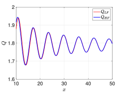
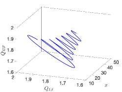
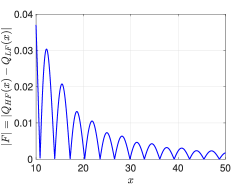
Figure 1: Motivation behind the new residual multi-fidelity formulation. Left: deviation of the low-fidelity solution $Q_{LF}$ from the high-fidelity solution $Q_{HF}$, versus a frequency parameter $\theta\in\Theta=[10,50]$. Middle: high-fidelity solution is not a linear function of the low-fidelity solution on the whole parameter space. Right: residual function $F$ has a small magnitude.

II. Small residual magnitude. It is important to note that we do not formulate the non-linearity discussed above as a direct relation between the two models, that is, we do not write $Q_{HF}(\bm{\theta})=F(\bm{\theta},Q_{LF}(\bm{\theta}))$. Instead, we formulate the non-linearity in terms of the residual (4). This is motivated by the fact that the residual is expected to have a small magnitude (or norm) relative to that of the high-fidelity quantity $Q_{HF}$; see Figure 1 (right). As an additional example, consider a low-fidelity model and a high-fidelity model obtained by a coarse and a fine discretization of some ODE/PDE problem, satisfying (3). Further, let $h_{LF}=s\,h_{HF}$ where $1<s<\infty$. Then using triangle inequality we can write

$$|F|=|Q_{HF}-Q_{LF}|\leq|Q-Q_{HF}|+|Q-Q_{LF}|\leq c(h_{HF}^{q}+h_{LF}^{q})\leq c\,(1+s^{q})h_{HF}^{q}\leq(1+s^{q})\varepsilon_{\text{TOL}}.$$

The last inequality follows by the choice $c\,h_{HF}^{q}\leq\varepsilon_{\text{TOL}}$, which implies $\varepsilon:=|Q-Q_{HF}|\leq\varepsilon_{\text{TOL}}$, as desired. Hence the size of the residual $|F|$ is proportional to the small quantity $\varepsilon_{\text{TOL}}$.

We conjecture that the small magnitude of the residual function, compared to the size of $Q_{HF}$, enables its accurate approximation by a ReLU network with a complexity lower than that of a network that accurately approximates a function of size $|Q_{HF}|$. This conjecture is motivated by two recent theoretical results. In [25] the authors consider Fourier feature ResNets, and they derive bounds on network generalization error directly proportional to the uniform norm of the target function and inversely proportional to the network degree of freedom. We hypothesize that a similar result holds for ReLU networks, and we support this hypothesis with numerical examples in Section 5. Moreover, in [31], the author relates the size of a Sobolev target function to ReLU network complexity. See section 4 for more details. Overall, the major advantage of our residual formulation, over learning the correlation between different fidelity models directly, is that the quantity being learned generally has small relative magnitude (or norm). Such a small target quantity can be learned by a network with low degree of freedom, which in turn requires less expensive high-fidelity training data.

In summary, the residual multi-fidelity formulation enables the construction of an efficient pair of networks where the first network, which learns the residual function $F$ is leveraged to train a second network that learns the target quantity $Q_{HF}$; see Section 3.2 for details.

3.2 Composite network training

The second major component of the RMFNN algorithm consists of constructing a pair of networks that work together. This construction proceeds in three steps.

Step 1. Data generation. We generate a set of $N=N_{I}+N_{II}$ points, $\bm{\theta}\in\Theta$, collected in two disjoint sets:

$$\Theta_{I}:=\{\bm{\theta}^{(1)},\dotsc,\bm{\theta}^{(N_{I})}\}\subset\Theta,\qquad\Theta_{II}:=\{\bm{\theta}^{(N_{I}+1)},\dotsc,\bm{\theta}^{(N)}\}\subset\Theta,\qquad\Theta_{I}\cap\Theta_{II}=\emptyset.$$

The points in each set may be selected deterministically or randomly. For example, the two sets may consist of two uniform or non-uniform disjoint grids over $\Theta$, or we may consider a random selection of points drawn from a probability distribution, such as a uniform distribution or other optimally chosen distribution. We then proceed with the following computations.

• For each $\bm{\theta}^{(i)}\in\Theta_{I}\cup\Theta_{II}$, with $i=1,\dotsc,N$, we compute the low-fidelity realizations,

  $$Q_{LF}^{(i)}:=Q_{LF}(\bm{\theta}^{(i)})=M_{Q}(\bm{u}_{h_{LF}}(\bm{x};\bm{\theta}^{(i)})),\qquad i=1,\dotsc,N.$$

• For each $\bm{\theta}^{(i)}\in\Theta_{I}$, with $i=1,\dotsc,N_{I}$, we compute the high-fidelity realizations,

  $$Q_{HF}^{(i)}:=Q_{HF}(\bm{\theta}^{(i)})=M_{Q}(\bm{u}_{h_{HF}}(\bm{x};\bm{\theta}^{(i)})),\qquad i=1,\dotsc,N_{I}.$$ (5)

Step 2. Composite network training. We train two separate networks as follows:

• Using $N_{I}$ input data, $\{(\bm{\theta}^{(i)},Q_{LF}^{(i)})\}_{i=1}^{N_{I}}$ and $N_{I}$ output data, $\{Q_{HF}^{(i)}-Q_{LF}^{(i)}\}_{i=1}^{N_{I}}$, we train an initial network ($ResNN$) to learn the residual function $F$ in (4). We call this surrogate $F_{ResNN}$; see Figure 2 (top).

• We then use the surrogate $F_{ResNN}$ and the rest of the $N_{II}$ low-fidelity data points $\{(\bm{\theta}^{(i)},Q_{LF}^{(i)})\}_{i=N_{I}+1}^{N}$ to generate $N_{II}$ new approximate high-fidelity outputs, denoted by $\{\hat{Q}_{HF}^{(i)}\}_{i=N_{I}+1}^{N}$, where

  $$\hat{Q}_{HF}^{(i)}:=Q_{LF}^{(i)}+F_{ResNN}(\bm{\theta}^{(i)},Q_{LF}^{(i)}),\qquad i=N_{I}+1,\dotsc,N.$$ (6)

• Using all $N$ input-output high-fidelity data $\{(\bm{\theta}^{(i)},Q_{HF}^{(i)})\}_{i=1}^{N_{I}}\cup\{(\bm{\theta}^{(i)},\hat{Q}_{HF}^{(i)})\}_{i=N_{I}+1}^{N}$, we train a deep network ($DNN$) as a surrogate for the high-fidelity quantity $Q_{HF}$. We call this surrogate $Q_{DNN}$; see Figure 2 (bottom).

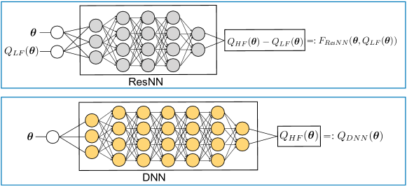
Figure 2: Schematic representation of the RMFNN algorithm, given a set of $N$ low-fidelity and $N_{I}\ll N$ high-fidelity data. Top: an initial network ($ResNN$) is trained by $N_{I}$ low-fidelity and high-fidelity data to learn the residual function $F$. The trained $ResNN$ is used along with the rest of $N_{II}=N-N_{I}$ low-fidelity data to generate a new set of $N_{II}$ high-fidelity data. Bottom: a deep network ($DNN$) is trained by all $N$ high-fidelity data as a surrogate for the high-fidelity target quantity $Q_{HF}$.

Step 3. Prediction. Given any $\bm{\theta}\in\Theta$, an approximation $\tilde{Q}(\bm{\theta})$ of the target quantity $Q(\bm{\theta})$ can be obtained by evaluating the trained deep network $DNN$:

$$\tilde{Q}(\bm{\theta})=Q_{DNN}(\bm{\theta}),\qquad\bm{\theta}\in\Theta.$$ (7)

On performance of RMFNN algorithm. It is important to note that the two networks learn two essentially different quantities: $ResNN$ learns the residual function $F$, while $DNN$ learns the target high-fidelity quantity ${Q}_{HF}$. On the one hand, since $F$ has small norm (as motivated in Section 3.1), it can be realized by a network of relatively low degree of freedom while keeping the approximation error small. On the other hand, ${Q}_{HF}$ likely has a larger norm than that of the residual function, and therefore it may need to be realized by a deeper network to achieve the desired accuracy. Importantly, this architectural difference between the two networks pairs well with the training data availability conditions present in most multi-fidelity modeling problems. Generally, the number $N_{I}$ of available high-fidelity data is small compared to the number $N$ of available low-fidelity data, i.e. $N_{I}\ll N$. Since $ResNN$ learns a quantity that is generally small in magnitude relative to the quantity learned by $DNN$, it can do so with a network of smaller degree of freedom, and as such needs less training data. Specifically, $ResNN$ uses the small high fidelity data set numbering $N_{I}$, while $DNN$ uses a much larger data set numbering $N$. This is an important advantage of the RMFNN algorithm over current composite algorithms [29, 30], where the networks in their composite settings learn similar quantities in terms of magnitude and hence have similar architectures that need comparable number of training data ($N_{I}\sim N$).

An alternative approach. We can take a slightly different approach as follows. The first step is the same as in Step 1 above, where we generate low-fidelity and high-fidelity data.

Next, in Step 2, we construct a composite network as follows:

• Using $N$ input-output data $\{(\bm{\theta}^{(i)},Q_{LF}^{(i)}\}_{i=1}^{N}$, we train a deep network ($DNN$) as a surrogate for $Q_{LF}$.

• Using $N_{I}$ input data $\{(\bm{\theta}^{(i)},Q_{LF}^{(i)})\}_{i=1}^{N_{I}}$ and $N_{I}$ output data $\{Q_{HF}^{(i)}-Q_{LF}^{(i)}\}_{i=1}^{N_{I}}$, we train a second network ($ResNN$) as a surrogate for the residual function $F$ in (4). Note that this part is the same as the first part of step 2 in the original approach, but with a change in the order of implementation.

• We build a composite network by combining $DNN$ and $ResNN$ as shown in Figure 3.

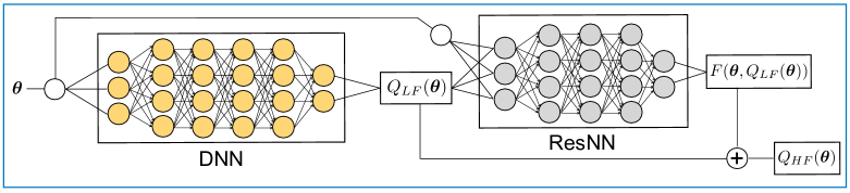
Figure 3: An alternative RMFNN approach. A deep network ($DNN$) is trained using $N$ low-fidelity data to learn $Q_{LF}$. A second network ($ResNN$) is trained by $N_{I}\ll N$ low-fidelity and high-fidelity data as a surrogate for the residual $F$. Finally, the target quantity $Q_{HF}$ is computed by adding $Q_{LF}$ to $F$.

For prediction in Step 3, given any $\bm{\theta}\in\Theta$, we compute an approximation $\tilde{Q}(\bm{\theta})$ of the target quantity $Q(\bm{\theta})$ by adding the low-fidelity quantity (predicted by $DNN$) to the residual (predicted by $ResNN$); see Figure 3.

A comparison between the two proposed approaches. Both approaches utilize the same residual multi-fidelity formulation (4), but they differ in the way their constituent networks ($ResNN$ and $DNN$) work. In the first approach, $ResNN$ and $DNN$ work at two separate stages: first, $ResNN$ learns the residual and generates more high-fidelity data; next, $DNN$ uses the initially available and newly generated high-fidelity data to learn the target quantity. In this case, $DNN$ alone serves as the surrogate network to be evaluated many times. In the alternative approach, $ResNN$ and $DNN$ constitute two blocks in a composite surrogate network, and hence both will be evaluated many times. In addition, since in both approaches $ResNN$ learns the same residual, and since $DNN$ learns either the low- or high-fidelity quantities, which are not expected to be very different in magnitude, we expect the architectures of $ResNN$ and $DNN$ to be comparable across both approaches. This gives each approach distinct benefits. When we need many evaluations of the target quantity, the alternative approach may be more expensive, because it requires both $DNN$ and $ResNN$ to be evaluated, compared to only one evaluation of $DNN$ in the first approach. The alternative approach, however, has the flexibility of replacing $DNN$ by a direct computation of $Q_{LF}$, for instance when a direct computation of $Q_{LF}$ is more economical compared to the cost of training and evaluating a surrogate network.

Comparison with residual networks. ResNets [21] were originally developed to address the degradation problem, a phenomenon where we observe an eventual decrease in network training accuracy as depth increases. ResNets addresses this problem by introducing shortcut connections that pass along identity maps between layers. In this, as the network depth increases and accuracy becomes saturated, additional layers need only learn a residual that tends to zero as opposed to the full identity map plus some small possibly nonlinear correction. Understood in the context of the recent theoretical results in [25], ResNets take advantage of learning a residual that is small (relative to the identity map) between each layer. It is important to note that the size of the residual, as formulated in ResNet, is only guaranteed to be small relative to the identity map when the network accuracy is close to saturated and the identity map is near optimal. This situation arises when considering the impact of adding additional layers to a deep neural network that already approximates the quantity of interest to a reasonable accuracy (the conditions of the degradation problem). In the context of multi-fidelity modeling, where the correlation between low-fidelity and high-fidelity models needs to be learned accurately on sparse training data, it is unreasonable to expect the residual between layers (as formulated in ResNet) to be small compared to the identity map. Therefore, in order to take advantage of the previously mentioned theoretical results, we need to explicitly enforce learning a small quantity. This is the exact insight of our proposed RMFNN algorithm. It formulates the correlational learning problem as learning a residual function $F$ between the high-fidelity and low-fidelity models, which is generally small relative to the high-fidelity quantity.

4 Theoretical Rationale for the RMFNN Algorithm

In this section we provide a detailed theoretical rationale for the RMFNN algorithm. We begin by discussing the sources of error incurred in using the RMFNN algorithm. We then review current theoretical results on the convergence rate of the approximation error and discuss the computational complexity of the algorithm.

4.1 Sources of error

Let $\varepsilon$ denote the error (1) in approximating $Q$ by the surrogate (7) obtained by the RMFNN algorithm, measured in $L^{2}$-norm, and satisfying the accuracy constraint

$$\varepsilon=||Q-Q_{DNN}||_{L^{2}(\Theta)}\leq\varepsilon_{\text{TOL}}.$$ (8)

By triangle inequality, we can split the error into three parts:

$$\varepsilon\leq\underbrace{||Q-Q_{HF}||_{L^{2}(\Theta)}}_{\varepsilon_{I}}+\underbrace{||Q_{HF}-\hat{Q}_{HF}||_{L^{2}(\Theta)}}_{\varepsilon_{II}}+\underbrace{||\hat{Q}_{HF}-Q_{DNN}||_{L^{2}(\Theta)}}_{\varepsilon_{III}}\leq\varepsilon_{\text{TOL}},$$

where the desired accuracy is achieved if, for instance, we enforce $\varepsilon_{I},\varepsilon_{II},\varepsilon_{III}\leq\frac{1}{3}\,\varepsilon_{\text{TOL}}$. The first error term $\varepsilon_{I}$ is the error in approximating $Q$ by $Q_{HF}$ in (5) using an ODE/PDE solver. Then, from (3) we have

$$\varepsilon_{I}\leq C\,h_{HF}^{q},$$

and hence we can meet the accuracy constraint if we select $h_{HF}$ such that $C\,h_{HF}^{q}\leq\frac{1}{3}\,\varepsilon_{\text{TOL}}$. The second and third error terms are errors in network approximation, and hence of a different nature. Indeed, the second error term $\varepsilon_{II}$ is the error in approximating $Q_{HF}$ by $\hat{Q}_{HF}$ in (6), which is the error in approximating $F$ in (4) by the ResNN surrogate $F_{ResNN}$,

$$\varepsilon_{II}=||Q_{LF}+F-Q_{LF}-F_{ResNN}||_{L^{2}(\Theta)}=||F-F_{ResNN}||_{L^{2}(\Theta)}.$$

The third error term $\varepsilon_{III}$ is the error in approximating $\hat{Q}_{HF}$ by the DNN surrogate $Q_{DNN}$. In general, the second and third error terms depend on three factors: i) the space of the target functions to be approximated, here the function space of $F$ and $Q_{HF}$; ii) the architectures of $ResNN$ and $DNN$ and their training hyperparameters, including, but not limited to, width, depth, activation functions, and the optimization algorithm and the cost function used in the training process; and iii) the quantity and distribution of the input training data for $ResNN$ and $DNN$, i.e. the choice of the sets $\Theta_{I}$ and $\Theta_{II}$.

It is to be noted that the precise dependence of the output error of a trained network on the target function space, network architecture, optimization hyperparameters, and the choice of input training data is still not completely understood, and one that we will not address here. Instead we address the computational complexity of training and evaluating the networks $ResNN$ and $DNN$ under the accuracy constraint $\varepsilon_{II}+\varepsilon_{III}\leq\frac{2}{3}\,\varepsilon_{\text{TOL}}$. In particular, we leverage two recent theoretical results to argue that, in general, for a given accuracy constraint, the complexity of the RMFNN algorithm is less than other state-of-the-art neural network-based surrogate construction methods.

4.2 Motivating theoretical results

Two recent theoretical results motivated the development of the RMFNN algorithm. The first is a result for Fourier feature residual networks [25]. In Theorem 2.1 of [25], the authors derive a bound on network generalization error directly proportional to the uniform norm of the target function and inversely proportional to the network degree of freedom. This result for Fourier features residual networks inspired the analogous conjecture for ReLU networks:

Conjecture 1.

Consider a target function $f\in L^{2}(\Theta)$ with bounded uniform norm $||f||_{\infty}<\infty$. Let $f_{\Phi}$ be a ReLU network’s output with trainable parameters $\Phi$ and consisting of $L$ layers and $K$ neurons in each layer. Then there is a constant $C>0$ such that

$$\min_{\Phi}||f-f_{\Phi}||_{L^{2}(\Theta)}^{2}\leq C\,\frac{||f||_{\infty}^{2}}{KL}+{\mathcal{O}}(K^{-2}+L^{-4}).$$ (9)

Proof of Conjecture 1 is the subject of ongoing research and will be presented elsewhere, but numerical evidence for such a bound is presented in section 5. Furthermore, the validity of a bound analogous to (9) for Fourier features residual networks supports the use of our residual multi-fidelity framework over the standard multi-fidelity framework used in [29, 30]. Indeed, for a fixed error tolerance, if we consider learning both the residual function $F(\bm{\theta},Q_{LF}(\bm{\theta}))=Q_{HF}(\bm{\theta})-Q_{LF}(\bm{\theta})$, which is generally small in uniform norm relative to $Q_{HF}$, and the direct mapping $G(\bm{\theta},Q_{LF}(\bm{\theta}))=Q_{HF}(\bm{\theta})$, we hypothesize that the former can be learned to the desired accuracy with considerably less network complexity than the latter. Moreover, the training of this network of smaller degree of freedom will generally require less training data, a quality that favorably addresses high-fidelity data sparsity conditions present in most multi-fidelity modeling problems.

Additional rationale for the RMFNN algorithm stems from Theorem 1, a recent result on approximation of Sobolev functions by ReLU networks, a proof for which can be found in [31]. For an in depth introduction to Sobolev function spaces we direct the reader to [12].

Theorem 1.

Let $\varepsilon_{\text{TOL}}\in(0,\frac{1}{2})$. Consider a Sobolev target function $f\in W^{k,p}(\Theta)$ on $\Theta=[0,1]^{d}$ with $k\geq 1$ and $p\in[1,\infty]$. Then there exists a ReLU neural network $f_{\Phi}$ with $d$ input neurons, one output neuron, and complexity

$$L(f_{\Phi}) \leq C\,\log_{2}(\varepsilon_{\text{TOL}}^{-1}\,||f||_{W^{k-1,p}(\Theta)}),$$

$$N(f_{\Phi}) \leq C\,\varepsilon_{\text{TOL}}^{-d/k}\,||f||_{W^{k,p}(\Theta)}^{d/k}\,\log_{2}^{2}(\varepsilon_{\text{TOL}}^{-1}\,||f||_{W^{k-1,p}(\Theta)}),$$

such that $||f-f_{\Phi}||_{L^{p}(\Theta)}\leq\varepsilon_{\text{TOL}}$. Here, $L(\Phi)$ and $N(\Phi)$ are the number of layers and the total number of neurons of the network $\Phi$, respectively, and the constant $C=C(d,k,p)>0$ is independent of $\varepsilon_{\text{TOL}}$.

Important in this theorem is the dependence of network complexity on the size of the target function $f$. For a fixed error tolerance $\varepsilon_{TOL}$, the smaller the quantities $||f||_{W^{k,p}}$ and $||f||_{W^{k-1,p}}$, the smaller degree of freedom required in approximating the ReLU network. Furthermore, it is important to note that the bound on $N(f_{\Phi})$ depends strongly on $d/k$, a value that balances problem input dimension $d$ and target function regularity $k$. The problem regime in which neural networks promise to be highly beneficial is when $d/k>>1$ (high problem dimension and/or very irregular target function). In this case, the network complexity is highly dependent on the ratio $||f||_{W^{k,p}}/\varepsilon_{TOL}$. That is, if extremely accurate predictions are required ($\varepsilon_{TOL}<<1)$, and network complexity is to remain controlled, then we must also require $||f||_{W^{k,p}}\approx\varepsilon_{TOL}$. This condition is rarely satisfied in real world problems, but minimizing $||f||_{W^{k,p}}$ can help greatly in reducing otherwise very large network complexity, and enabling accurate network training on sparser data sets.

4.3 Computational complexity

We will now discuss the computational complexity of the RMFNN algorithm, denoted by $W_{RMFNN}$, for approximating the target quantity $Q(\bm{\theta})$ at $N_{\bm{\theta}}$ distinct points $\bm{\theta}\in\Theta$, when $N_{\bm{\theta}}\gg 1$ is large. The complexity of the algorithm consists of two major parts: the cost of training the two networks $ResNN$ and $DNN$, which is assumed to be dominated by the cost of obtaining $N_{I}$ high-fidelity training data, and the cost of $N_{\bm{\theta}}$ evaluations of the deep network estimator (7). The total cost is hence assumed to be given by

$$W_{RMFNN}=N_{I}\,W_{HF}+N_{\bm{\theta}}\,W_{DNN},$$ (10)

where $W_{HF}$ denotes the computational cost of one evaluation of $Q_{HF}$ in (2), and $W_{DNN}$ denotes the cost of one evaluation of $DNN$. In what follows, we discuss the cost (10) of RMFNN algorithm and compare it with the cost of the following two approaches:

• HFM: direct sampling of the high-fidelity model without utilizing neural network-based surrogate construction or lower-fidelity information. Here the expensive high-fidelity ODE/PDE model is directly computed $N_{\bm{\theta}}$ times with cost,

  $$W_{HFM}=N_{\bm{\theta}}\,W_{HF}.$$ (11)

• HFNN: evaluation of a deep high-fidelity neural network surrogate that is constructed without leveraging lower-fidelity information. The high-fidelity surrogate network is trained on only $N$ high-fidelity data and evaluated $N_{\bm{\theta}}$ times with cost,

  $$W_{HFNN}=N\,W_{HF}+N_{\bm{\theta}}\,W_{DNN}.$$ (12)

The higher efficiency of the RMFNN method, compared to the above alternative approaches, relies on the following two conditions:

1) $N_{I}\ll N<N_{\bm{\theta}}$;      and     2) $W_{DNN}\ll W_{HF}$.

Clearly, these two conditions imply that $W_{RMFNN}\ll W_{HFNN}<W_{HFM}$. We address each of these conditions in the two observations below.

Observation 1: As motivated in Section 3.1, and supported with theoretical results in Section 4.2, the small norm of $F$ enables its accurate approximation by the network $ResNN$ with far less complexity than the deep network $DNN$ that approximates $Q_{HF}$. This implies that the number $N_{I}$ of expensive high-fidelity data needed to train $ResNN$ may be far smaller than the total number $N$ of data needed to train $DNN$, that is $N_{I}\ll N$. Moreover, in many scientific problems, we often need a very large number ($N_{\bm{\theta}}\gg 1$) of high-fidelity samples, implying $N<N_{\bm{\theta}}$. For example, when using Monte Carlo sampling to evaluate the statistical moments of random quantities, we require $N_{\bm{\theta}}={\mathcal{O}}(\varepsilon_{\footnotesize{\text{TOL}}}^{-2})$, since the statistical error in Monte Carlo sampling is known to be proportional to $N_{\bm{\theta}}^{-1/2}$ [14]. In such cases, the inequality $N<N_{\theta}$ holds provided $N={\mathcal{O}}(\varepsilon_{\footnotesize{\text{TOL}}}^{-p})$, with $p<2$. We note that there is currently no rigorous results that relate the number and distribution of input training data to the accuracy of neural networks. However, we have observed through numerical experiments that for the type and size of networks that we have studied, the number of data needed to train a network to achieve accuracy within $\varepsilon_{\footnotesize{\text{TOL}}}$ indeed grows with a rate milder than ${\mathcal{O}}(\varepsilon_{\footnotesize{\text{TOL}}}^{-2})$.

Observation 2: The evaluation of a neural network mainly involves simple matrix-vector multiplications and evaluations of activation functions. The total evaluation cost depends on the width and depth of the network and the type of activation used. Crucially, the network evaluation cost depends only mildly on the complexity of the underlying ODE/PDE problem. As can be seen in Theorem 1, approximating target functions with successively lower regularity or larger problem input dimension will require neural networks of higher complexity (larger width and or depth). However, when evaluating the neural network, this added complexity manifests only as additional simple matrix-vector operations and cheap evaluations of activation functions. In particular, for QoIs that can be well approximated by a network with several hidden layers and hundreds or thousands of neurons, we expect $W_{ResNN}<W_{DNN}\ll W_{HF}$. Indeed, in such cases, the more complex the high-fidelity problem, and the more expensive computing the high-fidelity quantity, the smaller the ratio $W_{DNN}/W_{HF}$.

It is to be noted that in the above discussion we have assumed that the cost of training $DNN$ is dominated by the cost of obtaining high-fidelity training data, neglecting the one-time cost of solving the underlying optimization problem in the training process. This will be a valid assumption, for instance, when the cost of solving the network optimization problem (e.g. by stochastic gradient descent) is negligible compared to the cost of $N_{\bm{\theta}}>>1$ high-fidelity model evaluations. In particular, we have observed through numerical experiments that as the tolerance decreases, and hence $N_{\bm{\theta}}$ increases, this one-time network training cost may become negligible compared to the cost of $N_{\bm{\theta}}$ high-fidelity solves. We further illustrate this in Section 5.

An illustrative example. We compare the costs (10), (11), and (12) on a prototypical UQ task. Let $\bm{\theta}$ be a random vector with a known and compactly supported joint probability density function (PDF), and suppose that we want to obtain an accurate expectation of the random quantity $Q=Q(\bm{\theta})$ within a small tolerance, $\varepsilon_{\footnotesize{\text{TOL}}}\ll 1$. To achieve this using MC sampling, recalling that the the statistical error in MC sampling is proportional to $N_{\bm{\theta}}^{-1/2}$ [14], we require $N_{\bm{\theta}}\propto\varepsilon_{\footnotesize{\text{TOL}}}^{-2}\gg 1$ samples. Now, suppose that $W_{HF}\propto h_{HF}^{-\gamma}$, where $\gamma>0$ is related to the time-space dimension of the underlying ODE/PDE problem and the discretization technique used to solve the problem. Then, noting $h_{HF}\propto\varepsilon_{\footnotesize{\text{TOL}}}^{1/q}$, we obtain $W_{HF}\propto\varepsilon_{\footnotesize{\text{TOL}}}^{-\gamma/q}$. Therefore, the cost (11) of directly computing the high-fidelity model $N_{\bm{\theta}}$ times is

$$W_{HFM}\propto\varepsilon_{\footnotesize{\text{TOL}}}^{-(2+\gamma/q)}.$$ (13)

Following observation 1 above, we assume $N\propto\varepsilon_{\footnotesize{\text{TOL}}}^{-p}$, with $p<2$. This assumption indicates that the dependence of number $N$ of training data on the tolerance $\varepsilon_{TOL}$ is milder than the dependence of number of MC samples on the tolerance. Furthermore, we assume $r:=N_{I}/N\ll 1$. Finally, following observation 2 above, we assume that the evaluation cost of the deep network $DNN$ is less than the cost of a high-fidelity solve, i.e. $W_{DNN}\propto\varepsilon_{\footnotesize{\text{TOL}}}^{-\hat{p}}$, with $\hat{p}<\gamma/q$, implying $W_{DNN}\ll W_{HF}$. With these assumptions, the cost (12) of using a purely high-fidelity network surrogate and the cost (10) of using a surrogate generated by the RMFNN algorithm read

$$W_{HFNN}\propto\varepsilon_{\footnotesize{\text{TOL}}}^{-(p+\gamma/q)}+\varepsilon_{\footnotesize{\text{TOL}}}^{-(2+\hat{p})}+\text{training cost},$$ (14)

$$W_{RMFNN}\propto r\,\varepsilon_{\footnotesize{\text{TOL}}}^{-(p+\gamma/q)}+\varepsilon_{\footnotesize{\text{TOL}}}^{-(2+\hat{p})}+\text{training cost}.$$ (15)

Comparing (13) and (14), and excluding training costs (see the discussion above), we get $W_{HFNN}\ll W_{HF}$, when $p<2$ and $\hat{p}<\gamma/q$. Furthermore, comparing (14) and (15), we get $W_{RMFNN}\ll W_{HFNN}$, when $r\ll 1$ and $\hat{p}<p+\gamma/q-2$.

5 Numerical examples

In this section we apply the proposed RMFNN algorithm to computing three parametric ODE/PDE problems, of which the latter two are borrowed from [30]. In all problems, the parameters are represented by an $d$-dimensional random vector $\bm{\theta}\in\Theta\subset{\mathbb{R}}^{d}$, with a known and bounded joint PDF, $\pi:\Theta\rightarrow{\mathbb{R}}_{+}$. For each parametric problem, we consider a desired output quantity $Q:\Theta\rightarrow{\mathbb{R}}$, being a functional of the ODE/PDE solution. Our main goal is to compute an accurate and efficient surrogate for $Q$, denoted by $Q_{DNN}$, given by (7). We will measure the approximation error using the weighted $L^{2}$-norm, as defined in (1) with $p=2$. We approximate the error by sample averaging, using $N_{\varepsilon}$ independent samples $\{\bm{\theta}^{(i)}\}_{i=1}^{N_{\varepsilon}}\in\Theta$ drawn from $\pi(\bm{\theta})$, and record the weighted mean squared error (MSE),

$$\varepsilon=\int_{\Theta}|Q(\bm{\theta})-Q_{DNN}(\bm{\theta})|^{2}\,\pi(\bm{\theta})\,d\bm{\theta}\approx\frac{1}{N_{\varepsilon}}\sum_{i=1}^{N_{\varepsilon}}|Q(\bm{\theta}^{(i)})-Q_{DNN}(\bm{\theta}^{(i)})|^{2}=:\varepsilon_{MSE}.$$ (16)

To facilitate a comparison of our algorithm with that of [30], two of our numerical examples involve computing the expectation of $Q$,

$${\mathbb{E}}[Q]:=\int_{\Theta}Q(\bm{\theta})\,\pi(\bm{\theta})\,d\bm{\theta},$$

by MC sampling. Due to the slow convergence of MC sampling, obtaining an accurate estimation may require a very large number ($N_{\bm{\theta}}\gg 1$) of realizations of $Q$, each of which requires an expensive high-fidelity ODE/PDE solve. We will approximate all $N_{\bm{\theta}}$ realizations of $Q$ by the proposed surrogate $Q_{DNN}$, built on far less than $N_{\bm{\theta}}$ number of ODE/PDE solves. This is an exemplary setting where we need many evaluations of $Q_{DNN}$. To this end, we generate $N_{\bm{\theta}}$ independent samples of $\bm{\theta}$, say $\{\bm{\theta}^{(i)}\}_{i=1}^{N_{\bm{\theta}}}$, according to the joint PDF $\pi(\bm{\theta})$ and approximate ${\mathbb{E}}[Q]$ by the sample mean of its approximated realizations computed by the RMFNN algorithm:

$${\mathbb{E}}[Q]\approx{\mathcal{A}}_{RMFNN}:=\frac{1}{N_{\bm{\theta}}}\sum_{i=1}^{N_{\bm{\theta}}}Q_{DNN}(\bm{\theta}^{(i)}).$$ (17)

We compare the complexity of (17) with that of a direct high-fidelity MC computation,

$${\mathbb{E}}[Q]\approx{\mathcal{A}}_{HF}:=\frac{1}{N_{\bm{\theta}}}\sum_{i=1}^{N_{\bm{\theta}}}Q_{HF}(\bm{\theta}^{(i)}).$$ (18)

In addition to the mean squared error (16), we also report the absolute and relative errors in expectations,

$$\varepsilon_{\text{abs}}:=|{\mathbb{E}}[Q(\bm{\theta})]-{\mathcal{A}}|,\qquad\varepsilon_{\text{rel}}:=|{\mathbb{E}}[Q(\bm{\theta})]-{\mathcal{A}}|/|{\mathbb{E}}[Q(\bm{\theta})]|,$$ (19)

where the estimator ${\mathcal{A}}$ is either ${\mathcal{A}}_{RMFNN}$ or ${\mathcal{A}}_{HF}$. We note that $\varepsilon_{abs}$ and $\varepsilon_{\text{rel}}$ contain both the deterministic error (due to approximating $Q$ by either $Q_{DNN}$ or $Q_{HF}$) and the statistical error (due to MC sampling of $Q_{DNN}$ or $Q_{HF}$). In the case of approximation $Q$ by $Q_{DNN}$, we can employ triangle inequality and write

$$\varepsilon_{abs}\leq\bigl{\lvert}\mathbb{E}[Q(\bm{\theta})-Q_{DNN}(\bm{\theta})]\bigr{\rvert}+\bigl{\lvert}\mathbb{E}[Q_{DNN}(\bm{\theta})]-\mathcal{A}_{RMFNN}\bigr{\rvert},$$

where the first (deterministic) term is indeed the error measured in the weighted $L^{1}$-norm, as given in (1) with $p=1$.

In all examples the closed-form solutions to the problems, and hence the true values of $Q(\bm{\theta})$, are known. We use these closed-form solutions to compute errors in the approximations, and we always compare the cost of different methods subject to the same accuracy constraint. All codes are written in Python and run on a single CPU. To construct neural networks we leverage Pytorch [34] in example 5.1, and Keras [5] in examples 5.2 and 5.3, both of which are open-source neural-network libraries written in Python. It is to be noted that all CPU times are measured by time.process_time() in Python, taking average of tens of simulations.

5.1 A bi-fidelity surrogate construction task

For our first numerical experiment, we conduct a surrogate construction task using bi-fidelity information. We consider a pulsed harmonic oscillator governed by the system of ODEs,

$$\dot{\bf u}(t)=A\,{\bf u}(t)+\cos(\omega\,t)\,{\bf b},\qquad{\bf u}=\begin{bmatrix}u_{1}\\ u_{2}\\ \end{bmatrix},\qquad A=\begin{bmatrix}-2&0\\ 0&-0.25\\ \end{bmatrix},\qquad{\bf b}=\begin{bmatrix}b_{1}\\ b_{2}\\ \end{bmatrix},$$ (20)

with initial solution $\mathbf{u}(0)=(1,20)^{\top}$. We consider four model parameters: the frequency $\omega\in[5,50]$, the oscillation time $t\in[0,6]$, and two pulse parameters $(b_{1},b_{2})\in[0,0.2]\times[4,4.5]$, forming a four-dimensional parameter vector $\bm{\theta}=(\omega,t,b_{1},b_{2})$. Our goal is to construct a surrogate for the kinetic energy of the system,

$$Q(\bm{\theta})=||{\bf u}(\bm{\theta})||_{2}=\bigl{(}u_{1}^{2}(\bm{\theta})+u_{2}^{2}(\bm{\theta})\bigr{)}^{1/2},\qquad\bm{\theta}=(\omega,t,b_{1},b_{2}).$$

To this end, we utilize multi-fidelity modeling as follows. For the high-fidelity model $Q_{HF}$ we leverage the exact analytic solution to (20), and for the low-fidelity model $Q_{LF}$ we employ an asymptotic method (see [7] and section 3.1) to derive a closed form asymptotic approximation. In Figure 4, the residual $F=Q_{HF}-Q_{LF}$ and the high-fidelity quantity $Q_{HF}$ are plotted for $b_{1}=0.2$ and $b_{2}=4.5$.

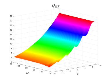
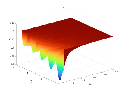
Figure 4: Profiles of $Q_{HF}$ (left) and $F$ (right) versus $(\omega,t)$ for $b_{1}=0.2$ and $b_{2}=4.5$.

We notice that in this example, both $Q_{HF}$ and $F$ are highly oscillatory, but $||F||_{\infty}\ll||Q_{HF}||_{\infty}$. This is, however, characteristic of many real-world multi-fidelity modeling problems, and it is discussed as a primary motivating factor for the RMFNN algorithm in section 3.1.

We will compare three different methods:

1. RMFNN ResNet: our proposed residual multi-fidelity algorithm using ReLU ResNets;

2. MFNN ResNet: the multi-fidelity framework proposed in [30] using ReLU ResNets;

3. HFNN ResNet: a single-fidelity ReLU ResNet trained on only high-fidelity data.

For the RMFNN algorithm we employ the alternative approach discussed in section 3.2, and, further, we replace the training of the deep network $DNN$ by direct evaluations of the low-fidelity model. As such, each of the three surrogate methods requires the training of just one neural network. For clarity, we state the mapping each of the methods learns below.

• RMFNN learns: $(\bm{\theta},Q_{LF}(\bm{\theta}))\mapsto(Q_{HF}(\bm{\theta})-Q_{LF}(\bm{\theta}))$

• MFNN learns: $(\bm{\theta},Q_{LF}(\bm{\theta}))\mapsto Q_{HF}(\bm{\theta})$

• HFNN learns: $\bm{\theta}\mapsto Q_{HF}(\bm{\theta})$

Across all three methods we use a fixed ReLU network architecture, with $L=7$ layers, $K=7$ neurons in each hidden layer, and one ReLU-free neuron in the last layer. Moreover, to facilitate a comparison of our residual multi-fidelity framework with standard ResNets [21], all ReLU networks are constructed with a ResNet-style architecture, where we implement shortcut connections that pass along the identity map every two layers. For each method, ReLU networks are trained on eleven different training sets where the number of high-fidelity (and low-fidelity) training samples ranges from 250 to 17000. These training sets are generated using a multi-variate uniform distribution over the parameter space. Moreover, the training sample inputs are normalized so that they reside in $\Theta=[0,1]^{4}$. For training, we use Adam optimization algorithm with the MSE cost function and Tikhonov regularization, and we implement an adaptive learning rate and stop criterion by monitoring the MSE on a validation set. To account for the randomness inherent in the training process, for each training set and for each surrogate method, we train and test 20 separate times on 20 distinct random seeds. From each train/test trial we compute the MSE (16) in the surrogate prediction on an independent test set of $N_{\varepsilon}=10^{6}$ points $\bm{\theta}$ uniformly distributed in $\Theta$. Figure 5 displays the average of the 20 MSEs versus the number of high-fidelity samples in the training set.

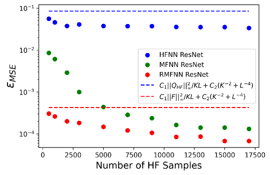
Figure 5: Mean squared error $\varepsilon_{MSE}$ in approximating $Q_{HF}$ by HFNN ResNet (blue), MFNN ResNet (green) and RMFNN ResNet (red) versus number of high-fidelity training samples.

As seen in Figure 5, RMFNN unilaterally outperforms the other methods, and this performance benefit is largest on sparse training data, the exact conditions desired in multi-fidelity computation. Further, the results highlight the importance of leveraging both of the motivating factors behind the RMFNN algorithm:

1. The method should leverage possibly non-linear correlations between low-fidelity and high-fidelity models.

2. The quantity that is learned during network training should ideally be small in magnitude relative to the high fidelity quantity of interest.

Table 1 describes the three surrogate methods in the context of properties (i) and (ii). A check mark indicates that the method satisfies the corresponding property.

methods	(i)	(ii)
HFNN
MFNN	$\checkmark$
RMFNN	$\checkmark$	$\checkmark$

Table 1: Comparison of RMFNN, MFNN, and HFNN methods in the context of properties (i) and (ii)

Property (i) is harnessed by both RMFNN and MFNN, and the orders of magnitude reduction in mean squared error for the MFNN method over the HFNN method verifies its importance. Continuing, property (ii) is characteristic of the RMFNN method, but not of the MFNN method. Hence the order of magnitude reduction in mean squared error achieved by RMFNN over MFNN validates the advantage of additionally learning a quantity of small norm relative to the high-fidelity quantity.

The red and blue dashed lines in Figure 5 are error bounds analogous to those proposed in Conjecture 1. Notice that the only difference between the blue and red dashed lines is the uniform norm appearing in the numerator of the first term. For the blue line, this is $||Q_{HF}||_{\infty}$, and for the red line, the residual $||F||_{\infty}$. Furthermore, the constants $C_{1}$ and $C_{2}$ were empirically chosen, but are importantly the same for both the blue and red dashed lines. As such, this numerical experiment provides preliminary evidence for Conjecture 1. A proof for this conjecture, as well as extensive numerical validation, is the subject of ongoing research.

The orders of magnitude reduction in error for the RMFNN ResNet over the HFNN ResNet also shows that our residual multi-fidelity framework makes a meaningful improvement over simply using ResNet-style shortcut connections in a single-fidelity network. In particular, these results support our discussion in Section 3.2, where we compare the residual formulation in ResNet [21] with our residual multi-fidelity framework. To reiterate, the residual learning formulated in ResNet does well in addressing the degradation problem, however; in a multi-fidelity context, it does not sufficiently take advantage of learning a quantity of small norm. On the contrary, the proposed RMFNN algorithm exploits this advantage to a much greater extent, enforcing the learning of such a quantity by leveraging multi-fidelity information.

It is important to note that while the results in Figure 5 were obtained for a fixed network architecture with $(K,L)=(7,7)$, the experiment was also conducted for $(K,L)=(25,7)$ and $(K,L)=(7,15)$. The results obtained for these different network architectures are analogous to those pictured in Figure 5 up to a universal and commensurate reduction in MSE across all surrogate methods. Such a reduction in error can be explained by an increase in the number of trainable parameters and hence in the expressive capacity of the networks.

5.2 A parametric ODE problem

Consider the following parametric initial value problem (IVP),

$$\begin{array}[]{ll}u_{t}(t,\theta)+0.5\,u(t,\theta)=f(t,\theta),&\qquad t\in[0,T],\\ u(0,\theta)=g(\theta),&\end{array}$$ (21)

where $\theta\in\Theta=[-1,1]$ is a uniformly distributed random variable. Using the method of manufactured solutions, we choose the force term $f$ and the initial data $g$ so that the exact solution to the IVP (21) is

$$u(t,\theta)=0.5+2\sin(12\theta)+6\sin(2t)\sin(10\theta)(1+2\theta^{2}).$$

Now consider the target quantity

$$Q(\theta)=|u(T,\theta)|,\quad T=100.$$

Our goal is to use the RMFNN algorithm to construct a surrogate $Q_{DNN}$ for $Q$, and then to employ MC sampling to compute the expectation ${\mathbb{E}}[Q(\theta)]$.

Multi-fidelity models and accuracy constraint. Suppose that we use the second-order accurate Runge-Kutta (RK2) time-stepper as the deterministic solver to compute realizations of $Q_{LF}(\theta)$ and $Q_{HF}(\theta)$ using time steps $h_{LF}$ and $h_{HF}$, respectively. We perform a simple error analysis, similar to the analysis in [30], to obtain the minimum number of realizations $N_{\theta}$ and the maximum time step $h_{HF}$ for the high-fidelity model to satisfy the accuracy constraint $\varepsilon_{\text{rel}}\leq\varepsilon_{\footnotesize{\text{TOL}}}$ with a $1\%$ failure probability, i.e. ${\text{Prob}}(\varepsilon_{\text{rel}}\leq\varepsilon_{\footnotesize{\text{TOL}}})=0.99$. Here $\varepsilon_{\text{rel}}$ is the relative error given in (19). Table 2 summarizes the numerical parameters $(N_{\theta},h_{HF},h_{LF})$ and the CPU time of evaluating single realizations of $Q_{LF}$ and $Q_{HF}$ for a decreasing sequence of tolerances $\varepsilon_{\footnotesize{\text{TOL}}}=10^{-2},10^{-3},10^{-4}$. We choose $h_{LF}=s\,h_{HF}$, with $s=5,10,10$, for the three tolerance levels.

Table 2: Required number of realizations and time steps to achieve ${\text{P}}(\varepsilon_{\text{rel}}\leq\varepsilon_{\footnotesize{\text{TOL}}})=0.99$.

$\varepsilon_{\footnotesize{\text{TOL}}}$	$N_{\theta}$	$h_{HF}$	$W_{HF}$	$h_{LF}$	$W_{LF}$
$10^{-2}$	$1.35\times 10^{5}$	0.1	$2.24\times 10^{-4}$	0.5	$4.36\times 10^{-5}$
$10^{-3}$	$1.35\times 10^{7}$	0.025	$7.21\times 10^{-4}$	0.25	$1.04\times 10^{-4}$
$10^{-4}$	$1.35\times 10^{9}$	0.01	$2.20\times 10^{-3}$	0.1	$2.24\times 10^{-4}$

Surrogate construction. Following the algorithm in Section 3.2, we first generate a set of $N=N_{I}+N_{II}$ points, $\theta^{(i)}\in[-1,1]$, with $i=1,\dotsc,N$, collected into two disjoint sets, $\Theta_{I}$ and $\Theta_{II}$. We choose the points to be uniformly placed on the interval $[-1,1]$. We select every 10th point to be in the set $\Theta_{I}$, and we collect the rest of the points in the set $\Theta_{II}$. This implies $N\approx 10\,N_{I}$, meaning that we need to compute the target quantity $Q(\theta)$ by the high-fidelity model (using RK2 with time step $h_{HF}$) at only 10% of points, i.e. $r=N_{I}/N\approx 0.1$; compare this with $r=0.25$ taken in [30] to achieve the same accuracy. The number of points $N$ will be chosen based on the desired tolerance, slightly increasing as the tolerance decreases, i.e. $N\propto\varepsilon_{\footnotesize{\text{TOL}}}^{-p}$ where $p>0$ is small. In particular, we observe in Table 3 below that the value $p=0.5$ is enough to meet our accuracy constraints.

The architecture of $ResNN$ consists of 2 hidden layers, where each layer has 10 neurons. The architecture of $DNN$ consists of 4 hidden layers, where each layer has 20 neurons. The architecture of both networks will be kept fixed at all tolerance levels. For the training process, we employ the MSE cost function and use Adam optimization technique. For both networks, we split the available data points into a training set (95$\%$ of data) and a validation set (5$\%$ of data) and adaptively tune the learning rate parameter. We do not use any regularization technique. Table 3 summarizes the number of training-validation data $N_{I}$ (for $ResNN$) and $N$ (for $DNN$), the number of epochs $N_{\text{epoch}}$, batch size $N_{\text{batch}}$, and the CPU time of training and evaluating the two networks for different tolerances. With these parameters we construct three surrogates for $Q_{DNN}$, one at each tolerance level. We note that while using a different architecture and other choices of network parameters (e.g. number of layers/neurons and learning rates) may give more efficient networks, the selected architectures and parameters here, following the general guidelines in [4, 16], produce satisfactory results in terms of efficiency and accuracy; see Table 4 and Figures 6-8 below.

Table 3: The number of training data and training and evaluation time of the two networks.

			$ResNN$: 2$\times$10 neurons				$DNN$: 4$\times$20 neurons
$\varepsilon_{\footnotesize{\text{TOL}}}$	$N_{I}$	$N$	$N_{\text{epoch}}$	$N_{\text{batch}}$	$W_{T_{1}}$	$W_{P_{1}}$	$N_{\text{epoch}}$	$N_{\text{batch}}$	$W_{T_{2}}$	$W_{P_{2}}$
$10^{-2}$	25	241	100	10	9.72	$2.98\times 10^{-5}$	400	40	35.24	$4.38\times 10^{-5}$
$10^{-3}$	81	801	1500	30	49.08	$2.98\times 10^{-5}$	8000	80	927.77	$4.38\times 10^{-5}$
$10^{-4}$	321	3201	5000	50	257.86	$2.98\times 10^{-5}$	20000	50	13708.08	$4.38\times 10^{-5}$

Table 4 reports the MSE (16) in the constructed surrogates $Q_{DNN}$ using $N_{\varepsilon}={10}^{8}$ evenly distributed points $\theta$ in $\Theta$, confirming that the (deterministic) MSE in the network approximation is comparable to the (statistical) relative error $\varepsilon_{\text{rel}}$.

Table 4: MSE in the approximation $Q_{DNN}(\theta)\approx Q(\theta)$.

$\varepsilon_{\footnotesize{\text{TOL}}}$	$\varepsilon_{MSE}$
$10^{-2}$	$2.25\times 10^{-2}$
$10^{-3}$	$1.50\times 10^{-3}$
$10^{-4}$	$1.40\times 10^{-4}$

Figure 6 shows the low-fidelity and high-fidelity quantities versus $\theta\in[-1,1]$ (solid lines) and the data (circle and triangle markers) available in the case $\varepsilon_{\footnotesize{\text{TOL}}}=10^{-2}$. Figure 7 (left) shows the generated high-fidelity data by the network $ResNN$, and Figure 7 (right) shows the predicted high-fidelity quantity by the deep network $DNN$ for tolerance $\varepsilon_{\footnotesize{\text{TOL}}}=10^{-2}$.

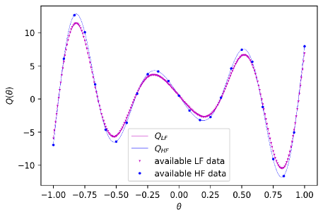
Figure 6: The low-fidelity and high-fidelity quantities versus $\theta\in[-1,1]$ (solid lines) and the available data (markers) in the case $\varepsilon_{\footnotesize{\text{TOL}}}=10^{-2}$. There are $N_{I}=25$ high-fidelity and $N=241$ low-fidelity data points, represented by circles and triangles, respectively.

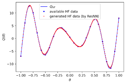
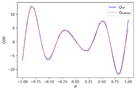
Figure 7: Outputs of the trained networks for $\varepsilon_{\footnotesize{\text{TOL}}}=10^{-2}$. Left: generated data by the network, $ResNN$. Right: predicted quantity by the deep network, $DNN$.

MC sampling. We next compute ${\mathbb{E}}[Q]$ by (17) and (18) and compare their complexities. Figure 8 (left) shows the CPU time as a function of tolerance. The computational cost of a direct high-fidelity MC computation (18) is ${\mathcal{O}}(\varepsilon_{\footnotesize{\text{TOL}}}^{-2.5})$, following (13) and noting that the order of accuracy of RK2 is $q=2$, and that the time-space dimension of the problem is $\gamma=1$. On the other hand, if we only consider the prediction time of the proposed residual multi-fidelity method, excluding the training costs, the cost is ${\mathcal{O}(\varepsilon_{\footnotesize{\text{TOL}}}^{-2})}$, which is much less than the cost of high-fidelity MC sampling. When adding the training costs, we observe that although for large tolerances the training cost is large, as the tolerance decreases, the training costs become negligible compared to the total CPU time. Overall, the cost of the proposed method approaches ${\mathcal{O}}(\varepsilon_{\footnotesize{\text{TOL}}}^{-2})$ as tolerance decreases, and hence, the smaller the tolerance, the more gain in computational cost when employing the proposed method over high-fidelity MC sampling. This can also be seen by (15) noting that $\max(p+\gamma/q,2+\hat{p})=\max(0.5+0.5,2+\hat{p},)=2+\hat{p}$, where $\hat{p}>0$ is very small. Finally, Figure 8 (right) shows the relative error as a function of tolerance for the proposed method, verifying that the tolerance is met with 1$\%$ failure probability.

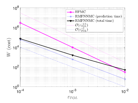
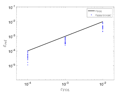
Figure 8: CPU time and error versus tolerance. Left: for large tolerances the training cost is dominant, making the cost of RMFNNMC more than the cost of HFMC. However, as tolerance decreases, the training cost becomes negligible and the cost of RMFNNMC approaches ${\mathcal{O}}(\varepsilon_{\footnotesize{\text{TOL}}}^{-2})$. Right: relative error as a function of tolerance verifies that the tolerance is met with 1$\%$ failure probability. The “+” markers correspond to 20 simulations at each tolerance level.

5.3 A parametric PDE problem

Consider the following parametric initial-boundary value problem (IBVP)

$$\begin{array}[]{ll}u_{tt}(t,\bm{x},\bm{\theta})-\Delta_{\bm{x}}u(t,\bm{x},\bm{\theta})=f(t,\bm{x},\bm{\theta}),&\ \ \ (t,\bm{x},\bm{\theta})\in[0,T]\times D\times\Theta,\\ u(0,\bm{x},{\bm{\theta}})=g_{1}({\bm{x}},\bm{\theta}),\ \ u_{t}(0,\bm{x},\bm{\theta})=g_{2}(\bm{x},\bm{\theta}),&\ \ \ (t,\bm{x},\bm{\theta})\in\{0\}\times D\times\Theta,\\ u(t,\bm{x},\bm{\theta})=g_{b}(t,\bm{x},\bm{\theta}),&\ \ \ (t,\bm{x},\bm{\theta})\in[0,T]\times\partial D\times\Theta,\end{array}$$ (22)

where $t\in[0,T]$ is the time, $\bm{x}=(x_{1},x_{2})\in D$ is the vector of spatial variables in a square domain $D=[-1,1]^{2}$, and $\bm{\theta}=(\theta_{1},\theta_{2})\in\Theta$ is a vector of two independently and uniformly distributed random variables on $\Theta=[10,11]\times[4,6]$. We select the force term $f$ and the initial-boundary data $g_{1},g_{2},g_{b}$ so that the exact solution to the IBVP (22) is

$$u(t,\bm{x},\bm{\theta})=\sin(\theta_{1}\,t-\theta_{2}\,x_{1})\,\sin(\theta_{2}\,x_{2}).$$

We consider the target quantity,

$$Q(\bm{\theta})=|u(T,\bm{x}_{Q},\bm{\theta})|,\qquad T=30,\qquad{\bf x}_{Q}=(0.5,0.5).$$

Our goal is to construct a surrogate $Q_{DNN}$ for $Q$ and then to compute the expectation ${\mathbb{E}}[Q(\bm{\theta})]$ by MC sampling.

Multi-fidelity models and accuracy constraint. Suppose that we have a second-order accurate (in both time and space) finite difference scheme as the deterministic solver to compute realizations of $Q_{LF}(\bm{\theta})$ and $Q_{HF}(\bm{\theta})$ using a uniform grid with grid lengths $h_{LF}$ and $h_{HF}$, respectively. We use the time step, $\Delta t=h/2$, to ensure stability of the numerical scheme, where the grid length $h$ is either $h_{LF}$ or $h_{HF}$, depending on the level of fidelity. Given a $1\%$ failure probability and a decreasing sequence of tolerances $\varepsilon_{\footnotesize{\text{TOL}}}=10^{-1},10^{-2},10^{-3}$, a simple error analysis, similar to the analysis in [30], and verified by numerical computations, gives the minimum number of realizations $N_{\bm{\theta}}$ and the maximum grid length $h_{HF}$ for the high-fidelity model required to achieve $\text{Prob}(\varepsilon_{\text{abs}}\leq\varepsilon_{\footnotesize{\text{TOL}}})=0.99$. Here, $\varepsilon_{\text{abs}}$ is the absolute error given in (19). Table 5 summarizes the numerical parameters $(N_{\bm{\theta}},h_{HF},h_{LF})$, and the CPU time of evaluating single realizations of $Q_{LF}$ and $Q_{HF}$. We choose $h_{LF}=s\,h_{HF}$, with $s=1.6,4,8$, for the three tolerance levels.

Table 5: Required number of realizations and grid lengths to achieve $\text{P}(\varepsilon_{\text{abs}}\leq\varepsilon_{\footnotesize{\text{TOL}}})=0.99$.

$\varepsilon_{\footnotesize{\text{TOL}}}$	$N_{\bm{\theta}}$	$h_{HF}$	$W_{HF}$	$h_{LF}$	$W_{LF}$
$10^{-1}$	$1.5\times 10^{2}$	$1/32$	$0.67$	$1/20$	$0.21$
$10^{-2}$	$1.5\times 10^{4}$	$1/128$	$29.75$	$1/32$	$0.67$
$10^{-3}$	$1.5\times 10^{6}$	$1/320$	$708.21$	$1/40$	$1.59$

Surrogate construction. Following the RMFNN algorithm in Section 3.2, we first generate a uniform grid of $N=N_{I}+N_{II}$ points $\bm{\theta}^{(i)}\in[10,11]\times[4,6]$, with $i=1,\dotsc,N$, collected into two disjoint sets $\Theta_{I}$ and $\Theta_{II}$. We select the two disjoint sets so that $N\approx 11\,N_{I}$, meaning that we need to compute the quantity $Q(\bm{\theta})$ by the high-fidelity model with grid length $h_{HF}$ at $9\%$ of points, i.e. $r=N_{I}/N\approx 0.09$; compare this with $r=0.25$ in [30]. The number $N$ of points will be chosen based on the desired tolerance, slightly increasing as the tolerance decreases, i.e. $N\propto\varepsilon_{\footnotesize{\text{TOL}}}^{-p}$ where $p>0$ is small. In particular, as we observe in Table 6 below, the value $p=0.2$ is enough to meet our accuracy constraints.

The architecture of $ResNN$ consists of 2 hidden layers, where each layer has 20 neurons. The architecture of $DNN$ consists of 4 hidden layers, where each layer has 30 neurons. The architecture of both networks will be kept fixed at all tolerance levels. For the training process, we split the available data points into a training set (95$\%$ of data) and a validation set (5$\%$ of data). We apply pre-processing transformations to the input data points before they are presented to the two networks. Precisely, we transform the points from $[10,11]\times[4,6]$ into the unit square $[0,1]^{2}$. We employ the quadratic cost function and use the Adam optimization technique with an initial learning rate, $\eta=0.005$. This learning rate is adapted during training by monitoring the MSE on the validation set. We do not use any regularization technique. Table 6 summarizes the number of training-validation data $N_{I}$ (for $ResNN$) and $N$ (for $DNN$), the number of epochs $N_{\text{epoch}}$, the batch size $N_{\text{batch}}$, and the CPU time of training and evaluating the two networks for different tolerances. With these parameters we construct three surrogates for $Q_{DNN}$, one at each tolerance level.

Table 6: The number of training data and training and evaluation time of the two networks.

			$ResNN$: 2$\times$20 neurons				$DNN$: 4$\times$30 neurons
$\varepsilon_{\footnotesize{\text{TOL}}}$	$N_{I}$	$N$	$N_{\text{epoch}}$	$N_{\text{batch}}$	$W_{T_{1}}$	$W_{P_{1}}$	$N_{\text{epoch}}$	$N_{\text{batch}}$	$W_{T_{2}}$	$W_{P_{1}}$
$10^{-1}$	324	3498	100	50	15.16	$5.13\times 10^{-5}$	200	50	284.54	$1.34\times 10^{-4}$
$10^{-2}$	451	4961	200	50	47.51	$5.13\times 10^{-5}$	500	50	1301.65	$1.34\times 10^{-4}$
$10^{-3}$	714	8003	1000	50	304.30	$5.13\times 10^{-5}$	4000	50	14825.28	$1.34\times 10^{-4}$

Table 7 reports the MSE (16) in the constructed surrogates $Q_{DNN}$, using a uniform grid of $N_{\varepsilon}={10}^{8}$ points $\bm{\theta}$ in $\Theta$, confirming that the (deterministic) MSE in the network approximation is comparable to the (statistical) absolute error $\varepsilon_{\text{abs}}$.

Table 7: Weighted mean squared error in the approximation $Q_{DNN}(\bm{\theta})\approx Q(\bm{\theta})$.

$\varepsilon_{\footnotesize{\text{TOL}}}$	$\varepsilon_{MSE}$
$10^{-1}$	$1.42\times 10^{-2}$
$10^{-2}$	$0.69\times 10^{-3}$
$10^{-3}$	$0.78\times 10^{-4}$

MC sampling. We now compute ${\mathbb{E}}[Q]$ by (17) and (18) and compare their complexities. Figure 9 (left) shows the CPU time as a function of tolerance. The computational cost of a direct high-fidelity MC sampling is proportional to $\varepsilon_{\footnotesize{\text{TOL}}}^{-3.5}$, following (13) and noting that the order of accuracy of the finite difference scheme is $q=2$, and that the time-space dimension of the problem is $\gamma=3$. On the other hand, if we only consider the evaluation cost of the RMFNN algorithm constructed surrogate, excluding the training costs, the cost of the proposed RMFNN method is proportional to $\varepsilon_{\footnotesize{\text{TOL}}}^{-2}$ which is much less than the cost of high-fidelity MC sampling. When adding the training costs, we observe that although for large tolerances the training cost is large, as the tolerance decreases the training costs become negligible compared to the total CPU time. Overall, the cost of the proposed method approaches ${\mathcal{O}}(\varepsilon_{\footnotesize{\text{TOL}}}^{-2})$ as tolerance decreases, indicating orders of magnitude acceleration in computing the expectation compared to high-fidelity MC sampling. This convergence rate can also be seen by (15), noting that $\max(p+\gamma/q,2+\hat{p})=\max(0.2+1.5,2+\hat{p})=2+\hat{p}$, where $\hat{p}>0$ is very small. Finally, Figure 9 (right) shows the absolute error as a function of tolerance for the proposed method, verifying that the tolerance is met with 1$\%$ failure probability.

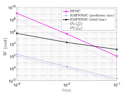
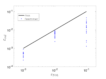
Figure 9: CPU time and error versus tolerance. Left: for large tolerances the training cost is dominant, making the cost of RMFNNMC more than the cost of HFMC. However, as tolerance decreases, the cost of RMFNNMC approaches ${\mathcal{O}}(\varepsilon_{\footnotesize{\text{TOL}}}^{-2})$. Right: error as a function of tolerance verifies that the tolerance is met with 1$\%$ failure probability. The “+” markers correspond to 20 simulations at each tolerance level.

6 Conclusion

In this work we presented a residual multi-fidelity computational framework that leverages a pair of neural networks to efficiently construct surrogates for high-fidelity QoIs described by systems of ODEs/PDEs. Given a low-fidelity and a high-fidelity computational model, we first formulate the correlation between the two models in terms of a possibly non-linear residual function that measures the discrepancy between the two model outputs. In section 4.2, we leveraged recent theoretical results [31, 25] to argue that the small magnitude (or norm) of the residual function, relative to the high-fidelity quantity, enables its accurate approximation by a neural network $ResNN$ of low relative complexity. Moreover, this low network complexity allows $ResNN$ to accurately learn the residual function on a sparse set of high-fidelity and low-fidelity data, the exact conditions encountered in most multi-fidelity modeling problems. The trained network $ResNN$ is then used to efficiently generate additional high-fidelity data. Finally, the set of all available and newly generated high-fidelity data is used to train a deep network $DNN$ that serves as a cheap-to-evaluate surrogate for the high-fidelity QoI.

We presented three numerical examples to demonstrate the power of the proposed framework. In example 5.1 we conducted a bi-fidelity surrogate construction task using 1) the RMFNN algorithm, 2) the MFNN method from [30], and 3) a pure high-fidelity neural network that does not leverage lower-fidelity information. We showed orders of magnitude reduction in generalization error for the RMFNN constructed surrogate over those constructed using the other two methods, and, further, demonstrated that this performance benefit is largest on sparse high-fidelity data. Furthermore, we showed that in a multi-fidelity context, our residual multi-fidelity framework makes a meaningful improvement over the residual learning framework as formulated in ResNet [21]. Continuing, in examples 5.2 and 5.3 we used our RMFNN constructed surrogate to approximate the expectation of our QoI via MC sampling. We exhibited large computational savings that are especially apparent when the output predictions are desired to be accurate within small tolerances.

This work inspires two primary future research directions. The first is a mathematical proof for Conjecture 1. Such a proof would be a natural and welcome addition to the numerical justification for the RMFNN algorithm presented in this manuscript. Moreover, it would facilitate a comparison between ReLU networks and Fourier feature networks on multi-fidelity modeling tasks.

The second future research direction concerns the extension of the RMFNN algorithm from bi-fidelity modeling to multi-fidelity modeling. The algorithm extends naturally in the case of an ensemble of lower-fidelity models that are strictly hierarchical. In this case, we leverage a sequence of networks to learn a sequence of residual functions that efficiently generate additional high-fidelity data.

7 Declarations

7.1 Data Availability

The datasets generated during and/or analysed during the current study are available from the corresponding author on reasonable request.

7.2 Competing Interests

The authors have no relevant financial or non-financial interests to disclose.

References

- [1] F. J. Anscombe and J. W. Tukey. The examination and analysis of residuals. Technometrics, 5:141–160, 1963.
- [2] R. C. Aydin, F. A. Braeu, and C. J. Cyron. General multi-fidelity framework for training artificial neural networks with computational models. Frontiers in Materials, 6:1–14, 2019.
- [3] A. R. Barron. Universal approximation bounds for superpositions of a sigmoidal function. IEEE Transactions on Information theory, 39:930–945, 1993.
- [4] Y. Bengio. Practical recommendations for gradient-based training of deep architectures. In Müller KR. Montavon G., Orr G.B., editor, Neural Networks: Tricks of the Trades, pages 437–478. Springer, Berlin, 2012.
- [5] François Chollet et al. Keras. https://keras.io, 2015.
- [6] K. A. Cliffe, M. B. Giles, R. Scheichl, and A. L. Teckentrup. Multilevel Monte Carlo methods and applications to elliptic PDEs with random coefficients. Comput. Visual Sci., 14:3–15, 2011.
- [7] M. Condon, A. Deaño, and A. Iserles. On systems of differential equations with extrinsic oscillation. Discrete & Continuous Dynamical Systems - A, 28:1345–1367, 2010.
- [8] I. Daubechies, R. A. DeVore, S. Foucart, B. Hanin, and G. Petrova. Nonlinear approximation and (deep) ReLU networks. arxiv.org/abs/1905.02199, 2019.
- [9] W. E, J. Han, and A. Jentzen. Algorithms for solving high dimensional PDEs: From nonlinear Monte Carlo to machine learning. arXiv:2008.13333, 2020.
- [10] W. E and B. Yu. The deep Ritz method: A deep learning-based numerical algorithm for solving variational problems. Commun. Math. Stat., 6:1–12, 2018.
- [11] D. Elbrächter, D. Perekrestenko, P. Grohs, and H. Bölcskei. Deep neural network approximation theory. arxiv.org/abs/1901.02220, 2019.
- [12] L. C. Evans. Partial Differential Equations, volume 19 of Graduate Studies in Mathematics. American Mathematical Society, Providence, Rhode Island, 1998.
- [13] M. G. Fernandez-Godino, C. Park, N. H. Kim, and R. T. Haftka. Review of multi-fidelity models. arXiv:1609.07196, 2016.
- [14] G. S. Fishman. Monte Carlo: Concepts, Algorithms, and Applications. Springer- Verlag, New York, 1996.
- [15] Alexander IJ Forrester, András Sóbester, and Andy J Keane. Multi-fidelity optimization via surrogate modelling. Proceedings of the royal society a: mathematical, physical and engineering sciences, 463(2088):3251–3269, 2007.
- [16] I. J. Goodfellow, Y. Bengio, and A. Courville. Deep Learning. MIT Press, Cambridge, MA, USA, 2016.
- [17] P. Grohs and L. Herrmann. Deep neural network approximation for high-dimensional elliptic PDEs with boundary conditions. arxiv.org/abs/2007.05384, 2020.
- [18] P. Grohs, F. Hornung, A. Jentzen, and P. von Wurstemberger. A proof that artificial neural networks overcome the curse of dimensionality in the numerical approximation of Black-Scholes partial differential equations. arxiv.org/abs/1809.02362, 2018.
- [19] I. Gühring, G. Kutyniok, and P. Petersen. Error bounds for approximations with deep ReLU neural networks in norms. Analysis and Applications, 18:803–859, 2020.
- [20] A.-L. Haji-Ali, F. Nobile, and R. Tempone. Multi-index Monte Carlo: when sparsity meets sampling. Numerische Mathematik, 132:767–806, 2016.
- [21] K. He, X. Zhang, S. Ren, and J. Sun. Deep residual learning for image recognition. In IEEE Conference on Computer Vision and Pattern Recognition, pages 770–778, 2016.
- [22] K. Hornik, M. Stinchcombe, and H. White. Multilayer feedforward networks are universal approximators. Journal Neural Networks, 2:359–366, 1989.
- [23] M. Hutzenthaler, A. Jentzen, T. Kruse, and T.A. Nguyen. A proof that rectified deep neural networks overcome the curse of dimensionality in the numerical approximation of semilinear heat equations. SN Partial Differential Equations and Applications volume, 1, 2020.
- [24] A. Jentzen, D. Salimova, and T. Welti. A proof that deep artificial neural networks overcome the curse of dimensionality in the numerical approximation of Kolmogorov partial differential equations with constant diffusion and nonlinear drift coefficients. arxiv.org/abs/1809.07321, 2018.
- [25] A. Kammonen, J. Kiessling, P. Plecháč, M. Sandberg, A. Szepessy, and R. Tempone. Smaller generalization error derived for a deep residual neural network compared with shallow networks. IMA Journal of Numerical Analysis, 2022.
- [26] M. C. Kennedy and A. O’Hagan. Predicting the output from a complex computer code when fast approximations are available. Biometrika, 87:1–13, 2000.
- [27] G. Kutyniok, P. Petersen, M. Raslan, and R. Schneider. A theoretical analysis of deep neural networks and parametric PDEs. arxiv.org/abs/1904.00377, 2019.
- [28] D. Liu and Y. Wang. Multi-fidelity physics-constrained neural network and its application in materials modeling. Journal of Mechanical Design, 141:121403, 2019.
- [29] X. Meng and G. E. Karniadakis. A composite neural network that learns from multi-fidelity data: Application to function approximation and inverse PDE problems. Journal of Computational Physics, 401: 20160751, 2020.
- [30] M. Motamed. A multi-fidelity neural network surrogate sampling method for uncertainty quantification. International Journal for Uncertainty Quantification, 10:315–332, 2020.
- [31] M. Motamed. Approximation power of deep neural networks: an explanatory mathematical survey. arXiv:2207.095511, 2022.
- [32] M. Motamed and D. Appelö. A multi-order discontinuous Galerkin Monte Carlo method for hyperbolic problems with stochastic parameters. SIAM J. Numer. Anal., 56:448–468, 2018.
- [33] F. Nobile and F. Tesei. A multi level Monte Carlo method with control variate for elliptic PDEs with log-normal coefficients. Stoch PDE: Anal Comp, 3:398–444, 2015.
- [34] Adam Paszke, Sam Gross, Francisco Massa, Adam Lerer, James Bradbury, Gregory Chanan, Trevor Killeen, Zeming Lin, Natalia Gimelshein, Luca Antiga, Alban Desmaison, Andreas Köpf, Edward Yang, Zach DeVito, Martin Raison, Alykhan Tejani, Sasank Chilamkurthy, Benoit Steiner, Lu Fang, Junjie Bai, and Soumith Chintala. Pytorch: An imperative style, high-performance deep learning library, 2019.
- [35] P. Perdikaris, M. Raissi, A. Damianou, N. Lawrence, and G. E. Karniadakis. Nonlinear information fusion algorithms for data-efficient multi-fidelity modelling. Proc. R. Soc. A, 473: 20160751, 2017.
- [36] P. Petersen and F. Voigtländer. Optimal approximation of piecewise smooth functions using deep ReLU neural networks. Neural Networks, 108:296–330, 2018.
- [37] A. Pinkus. Approximation theory of the MLP model in neural networks. Acta Numer., 8:143–195, 1999.
- [38] O. San and R. Maulik. Neural network closures for nonlinear model order reduction. Advances in Computational Mathematics, 44:1717–1750, 2018.
- [39] J. Schmidhuber. Deep learning in neural networks: An overview. Neural netw., 61:85–117, 2015.
- [40] J. Sirignano and K. Spiliopoulos. DGM: A deep learning algorithm for solving partial differential equations. Journal of Computational Physics, 375:1339–1364, 2018.
- [41] J. Willard, X. Jia, S. Xu, M. Steinbach, and V. Kumar. Integrating physics-based modeling with machine learning: A survey. arXiv:2003.04919, 2020.
- [42] D. Yarotsky. Error bounds for approximations with deep ReLU networks. Neural Networks, 94:103–114, 2017.