Proton synchrotron, plausible explanation for delayed VHE activity of 3C 279 in 2018

Abstract

A nearly 11-day delayed very-high-energy(VHE) activity compared to the Fermi-LAT flare from quasar 3C 279 was reported by H.E.S.S. on 28 January 2018. 3C 279 has long been considered a candidate site for particle acceleration; hence such events may embed information about the high-energy phenomena. We propose the production channel being leptonic for the multi-wavelength flare, UV-Optical-Xrays-$\gamma$-rays, whereas the delayed VHE activity originated from the proton synchrotron. Our model requires the magnetic field to be 2.3 G and the proton luminosity (L_p) $1.56\times 10^{46}$ erg/sec, whereas the lepton luminosity (L_e) $3.9\times 10^{43}$ erg/sec.

I Introduction

The observation of TeV-PeV neutrinos from blazar TXS 0506+056 [1], and Seyfert NGC 1068 [2] has encouraged hadronic emission studies from active galactic nuclei (AGNs). The brightest flat spectrum radio quasar (FSRQ) 3C 279 is a candidate source of hadronic emission as it has been recognized as a potential gamma-ray source at a distance z= 0.536[3]. In addition to being the first FSRQ observed above 100 GeV[4], 3C 279 was the first blazar demonstrating strong and rapid variability at GeV energy detected by EGRET onboard Compton Gamma Ray Observatory (CGRO)[5]. Even the rapid variability was observed at 0.1 to 300 GeV energy by the Fermi Large Array Telescope (LAT) with distinct giant flares [6, 7, 8, 9]. The source was first observed with very high energy (VHE) $\gamma$-rays by MAGIC on January 16, 2007, with a significance of 5.4$\sigma$ of flux $(3.8\pm 0.8)\times 10^{-11}$ ph $cm^{-2}s^{-1}$ above 150 GeV energy [10]. From December 2013 to April 2014, this source underwent a series of discrete flares, with the highest one-day average flux $(6.54\pm 0.30)\times 10^{-6}$ photons $cm^{-2}s^{-1}$ on 3 April 2014 [6]. Also, in June 2015, 3C 279 reported a record-breaking outburst with a daily flux level of $(2.45\pm 0.05)\times 10^{-5}$ photons $cm^{-2}s^{-1}$ at GeV energies [11]. and one of the flaring events of this time displayed an extremely harsh gamma-ray index[7]. Additionally, in 2015, a time scale variation of one hour was seen[8]. After PKS 1222+216, it is the second FSRQ-type blazar reported with a comparable brief minute-scale flux variation[9].

Dedicated attempts for modeling the source over all the wavelengths have been made with a) leptonic single zone, where optical to X-ray emission is explained with lepton synchrotron whereas VHE emission is explained with (SSC) [10], b) leptonic two/multi zones [10, 12] and c) lepto-hadronic channels for different observational epochs [13].

Interestingly, on 15 January 2018, Fermi-LAT reported the peak of an intense gamma-ray flare with flux $(8.4\pm 0.5)\times 10^{-6}$ photons $cm^{-2}$ $s^{-1}$[14]. As a follow-up observation of this flare Rapid Eye Mount telescope (REM) observed optical and near infra-red(NIR) wavelength of magnitude $V=14.39\pm 0.05$, $R=13.96\pm 0.14$, $I=13.37\pm 0.08$ $J=12.10\pm 0.02$, $H=11.27\pm 0.04$, $K=10.27\pm 0.04$[15]. The Astronomical Observatory of the University of Siena also reported an increase in R-band magnitude comparable with R-band measurement observation by the REM telescope on 17 January. Astro rivelatore Gamma a Immagini Leggero (AGILE) observed an increase of flux $(1.8\pm 0.3)\times 10^{-5}$ph $cm^{-2}s^{-1}$ $(E>100\,\text{MeV})$ at a significance level higher than 12$\sigma$[16]. The Dark Matter Particle Explorer (DAMPE) has also reported an increase in photon flux of $~{}(6.45\pm 3.63)\times 10^{-7}$ photons $cm^{-2}$$s^{-1}$ [17] after January 16, above 2 GeV. A nearly two-week follow-up search of TeV gamma-ray by the High Energy Stereoscopic System(H.E.S.S) observatory resulted in events above 100 GeV during January 27-28 with 11$\sigma$ [18], whereas, no events were observed during previous nights. So, this flare in very high energies (VHE) can be considered as at least 11 days delayed from the Fermi-LAT flare peak, marking it as an orphan flare. Hence, this event can be considered similar to the neutrino source TXS0 506+056 reported in [19]. In [20], this activity is explained through the interaction of the proton with the external photons.

A number of groups have explained the 2018 multi-wavelength high energy flare with leptonic model [21, 22]. While [21] studied the broadband variability of the source with electron synchrotron and inverse Compton (IC) scattering from the external photon field of broad line region (BLR) and disk region, [22] explained the IC and SSC from external torus region. [23] has explained the time delay of the H.E.S.S observations from the Fermi-LAT events with the lepto-hadronic synchrotron mirror model. The original model is explained in [24], where the VHE events originated from $\pi^{0}$ decay following p-$\gamma$ pion production. The candidate photon field is the Doppler blueshifted primary synchrotron photons that are reflected by a nearby mirror cloud.

To explain the approximate 11 days of delay of VHE Orphan flare from the Fermi-LAT HE flare, we used the same mechanism as in [19]. Due to heavier mass, proton synchrotron emission is delayed from electron synchrotron. Here, we explain the multi-wavelength emission from optical to HE with single-zone lepton synchrotron and Compton scattering of external photon field(EC) by BLR and disk region, whereas the delayed VHE emissions as a result of proton synchrotron.

We arrange the paper as follows: section II contains the details of the multiwavelength observation. This section also contains the study of the Fermi-LAT data for 3C 279 and the multi-wavelength data collected for various detectors. Section III contains the lepto-hadronic modeling for the epoch 14 January 2018 to 22 January 2018. A detailed explanation of the result is discussed in section IV.

II Multi-wavelength Observation of 3C 279

We collected the multi-wavelength data of radio, optical, and X-rays for quasar 3C 279 synchronized with the Fermi-LAT flare from 14 January 2018 to 22 January 2018 from [22]. The details of observation time for the multi-wavelength are listed in Table-1. The HE data detected by FERMI-LAT is again analyzed here for better understanding. We extract the VHE light curve data observed by H.E.S.S from in[23].

Table 1: Multiwavelength observations of 3C 279 blazar with observation time

Detectors	Time(MJD)	Reference
SARA-KPNO	$58137$	[25]
REM	$58135$	[15]
Swift XRT	$58135$ to $58140$	[22]
Fermi-LAT	$58131$ to $58142$	[14]
AGILE	$58136$	[16]
H.E.S.S	$58142$ to $58149$	[18]

II.1 Fermi-LAT HE light-curve of 3C 279

The HE light curve for the time MJD 58130-58142 (2018 January 12 to 2018 January 24) from 3C 279 as observed by Fermi-LAT is generated using Fermitool of Fermi-LAT light curve repository(LCR) with one-day bin for the energy range 0.1-300 GeV. In the analysis, we consider the region of interest (ROI)$10^{\circ}$, and the spectral shapes of sources within the region are variable. Our analysis suggests this source was in a flaring state between MJD 58132-58140 with the peak flux 3.82${\pm}$0.23 $\times$ $10^{-5}$ at time MJD 58135.9${\pm}$.4106. We calculate the rise time and the decay time of the Fermi flare by fitting HE Fermi $\gamma$-ray light curve with the following function [26]

$$F(t)=F_{b}+F_{0}\left(\frac{exp(t_{0}-t)}{T_{r}}+\frac{exp(t-t_{0})}{T_{d}}\right)^{-1},$$ (1)

where $F_{b}$ is the constant base flux and the photon flux is $F_{0}$ at time $t_{0}$, and $T_{r}$, $T_{d}$ are the rise time and decay time of the HE $\gamma$-ray peak.

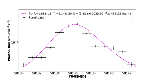
Figure 1: The Fermi-LAT $\gamma$-ray light curve (LC) of 3C 279 Quasar in the energy range 0.1 to 300 GeV between MJD 58130-58142 in the one-day bin.

The flare period can be calculated as ${2}(T_{d}+T_{r})$  [26]. The fitting 1 gives the rising and decay time as $1.61\pm.182$ and $2.14\pm.300$ days respectively and peak time, $t_{0}=58135.9\pm.410$. Hence, the flare period is nearly 6 days. Figure 1 shows the details of the HE $\gamma$-ray light curve and the analysis results.

II.2 Spectral Energy Distribution (SED) of HE energy Fermi-LAT flare

To construct the SED for HE emission of the source 3C 279 we first collected Fermi-LAT data in the energy range 0.1-300 GeV for the time period MJD 58130-58142 within ROI 10^∘ centred at the location of the source. We then performed an unbinned maximum-likelihood analysis using the standard software package Fermitool of version 2.2.0 and the instrument response function P8R2_SOURCE_V6 of Fermipy tool using Python user-contributed ENRICO script. All the parameters of the Galactic diffuse model (gll_iem_v07.fits) and isotropic component iso_P8R3_SOURCE_V3_v06.txt are kept free within a radius of 5^∘ for the analysis. In the event section Front+Back event type (evtype=3), evclass =128, and a zenith angle cut of 90^∘ are applied based on 8 pass reprocessed source class.

We chose the best-fit model among Single power law(PL), broken power law(BLP), and log-parabola(LP) for which the Akaike Information Criterion(AIC) [27] per degree of freedom is minimum. The details of the fitting parameters for the three models with their AIC values are given in table 2. We found that the difference in the AIC values of the LP model and the BPL model is not more than 2. This indicates both are acceptable models. Using Ochkam’s razor, we selected the LP model with fewer free parameters for the SED modelling for 3C 279 quasar. The extracted SED points are shown in figure 3 with the circle (green).

II.3 SED of VHE activity observed by H.E.S.S

As the details of the SED for the VHE emission during MJD 58142 to 58149 are unavailable, we extracted the spectrum from the light curve given in [23]. We assume the observed VHE follows a power-law in energy, $dN/dE_{\gamma}\propto(E_{\gamma}/E_{\gamma,0})^{-\alpha_{\gamma}}$. We normalized with the light curve to get the spectrum. We used $E_{0}=200$ GeV and the spectral index ${\alpha_{\gamma}}=4.1\pm 0.68$ to do the normalization. This assumption is based on the highest VHE activity observed for the quasar 3C 279 during January 2006 [4]. We show the SED of the VHE activity with the shaded region (blue) in figure 3 within the energy range 60 GeV to 500 GeV.

The SED for UV, optical, and X-ray wavelength events from [22]. The Swift UVOT and X-ray telescope (XRT) events are analyzed for 10 epochs from 2018 January 17 to 2018 February 1. The analysis details can be found in [22].

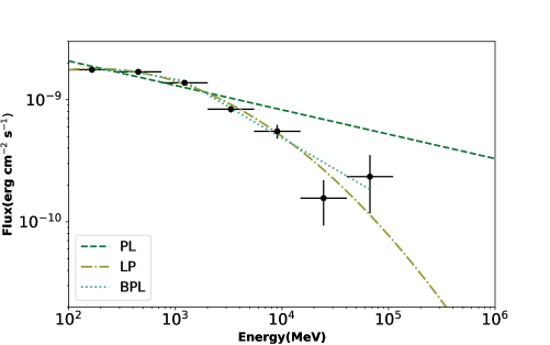
Figure 2: The HE Fermi data fitted with three different models PL, BPL and LP and details of the fitting parameters are given in Tabel 2

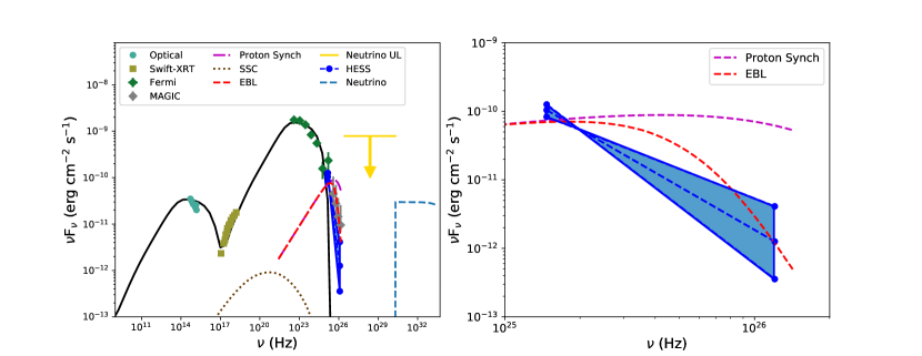
Figure 3: Multi-wavelength Modeling of 3C 279 quasar. The (cyan) circles for optical observations, (brown) square points for X-ray observation, green rectangle points for FERMI-LAT HE $\gamma$-ray observations and for VHE H.E.S.S observation, photon flux from the light curve in[18] has been extracted, multiplied with 60 GeV and assumed to be same for the energy range 60 GeV to 10 GeV, which is indicated by the red lines. SED Modeling: The electron synchrotron and IC scattering from BLR and disk region are shown with a (black) solid line, and the red dashed dot represents the proton synchrotron contribution. The gamma-ray emission after EBL contribution is shown with the (red) dashed line.

Model	$\alpha 1$	$\alpha 2$	beta	N0($10^{-10}$ TeV-1 cm-2 s-1)	TS	AIC
PL	$2.20{\pm}0.01$	$--$	$--$	$8.18\pm.16$	26490.10	157820
BPL	$2.07{\pm}0.01$	$2.51{\pm}0.04$	$--$	$9.81{\pm}.009$	$26730.39$	$157752$
LP	$2.14{\pm}0.01$	$--$	$0.07{\pm}0.01$	$1.01\pm.91$	$26687.13$	$157754$

Table 2: Best fitted parameters from Fermi-LAT analysis during the time period MJD 58130-58142 for three different models, Power law(PL), Broken Power law(BPL), and LogParabola(LP).Row 1: model name and 2, 3, and 4 are spectral indexes for distribution 4: Normalization constant 5: TS value 6: AIC values

III Lepto-Hadronic Model to explain the HE and VHE activity

In our model, we consider the accelerated leptons and hadrons in a single blob of the jet radiate while passing through the shell-like border of the broad line region (BLR). Considering the Doppler factor, $\delta$, and Lorentz factor, $\Gamma\sim\delta/2$ of the blob, one can calculate the emission region as $R_{em}=2c\Gamma^{2}t_{var}/(1+z)$. We modeled 3C 279 for $\delta=27$, which is above the minimum Doppler factor required for the escape of $\gamma$-rays around 500 GeV [28] and $\Gamma=\delta/2$. the emission region distance becomes $R_{em}\sim 7\times 10^{17}cm$ for a variability $t_{var}=1.14$ days (as reported in [21]). The BLR and Infra-red(IR) torus region can be assumed at a distance, $R_{BLR}=10^{17}L^{1/2}_{d,45}\sim 1.414\times 10^{17}\text{cm}$ and $R_{IR}=2.5\times 10^{18}L^{1/2}_{d,45}\sim 3.53\times 10^{18}\text{cm}$ [29] respectively, where $L_{d,45}$ is the disk (UV) luminosity in the units $10^{45}\text{erg/sec}$ [30]. Hence, we can safely consider our emission region to be towards the border of the BLR region, and the modeling may not include the torus region. Even though a long debate still continues around this [22, 21, 11][31].

The light curve of HE and VHE activity suggests an almost 6-day HE-flare approximately from MJD 58133 to MJD 58137 with the peak around MJD 58135.9 and a VHE activity as observed by H.E.S.S from MJD 58142 to 58149 with a peak flux around MJD 58146.5 figure 5. Hence, the observation of an 8 to 12-day delay in VHE activity from HE flare can be claimed. The shadow region (blue) of figure 5 also confirms no HE- activity is observed during the VHE activity. Using the above environment of the source 3C 279 we model the multi-wavelength observation from UV, Optical to soft X-rays as electron synchrotron emissions, whereas the HE- flare with the electron EC by the BLR and disk region photons. We use proton synchrotron emissions to explain the delayed VHE activity.

III.1 Lepton Modeling till HE gamma-rays

We model the flare MJD 58132-58140 of the multi-messengers starting from UV and optical to X-ray with synchrotron emissions from injected LP spectrum of accelerated electron while the HE $\gamma$-rays with their EC by the BLR and disk photons. Using the light curve analysis, we considered the total lepton emission period as $\text{age}=6\,\delta/(1+z)$ days. To calculate the propagated electron spectrum from the time-dependent transport equation for an injected LP model, we used the publicly accessible ”GAMERA” code [32]. The injected electron spectrum follows, ${N_{0}}(E_{e}^{\prime}/E_{ref}^{\prime})^{-(\alpha_{e}+{\beta_{e}}ln(E_{e}^{\prime}/E_{ref}^{\prime}))}$, where $E_{e}^{\prime}\text{and}E_{ref}^{\prime}$ are the electron energy and reference energy respectively. Hence Gamera takes $\gamma^{\prime}_{min}$, $\gamma^{\prime}_{max}$, spectral index $(\alpha_{e},\beta_{e})$ and the number of electrons per unit energy$(N_{0})$ as an input parameter. We calculate the synchrotron and EC-emitted radiations from the propagated electron spectrum. Here,^′ represents parameters in the jet frame.

The synchrotron emission from the propagated electron best fits the observed UV, Optical messengers for a magnetic field, B^′= 2.3 G. The EC for Klein-Nishina to explain the observed hard X-ray and HE photns is calculated for the BLR region with photon density $U^{\prime}_{BLR}$=9.67 erg/cm³ at a temperature $T^{\prime}_{BLR}=1.3\times 10^{4}$ K and U${}^{\prime}_{disk}=7\times 10^{-7}$ erg/cm³ (following [33]) and T${}^{\prime}_{disk}=2.3\times 10^{6}$ K, where the radius of the emission region, R${}^{\prime}=2\times 10^{16}$ cm. The photon density of the BLR region can be expressed as, $U^{\prime}=(1+\beta^{2})\Gamma^{2}L_{d}\eta_{BLR}/4\pi cR_{BLR}^{2}$, where $\eta_{BLR}$ is the fraction of disk luminosity transferred to BLR region. To achieve our requirement for better model fitting, we insist on the value of $\eta_{BLR}\sim 0.1$ (10 $\%$) [34]. The lepton modelling of the SED for the multi-wavelength observations is presented in figure 3, and the modelling parameters are listed in table 3

III.2 Hadron modeling for VHE gamma-rays activity

The emission region can be assumed to contain positively charged hadrons (here, we considered only protons) in addition to electron-positron pairs. The accelerating protons follow the non-thermal distribution $E_{p}^{\prime-\alpha_{p}}$ with an exponential cut-off. The relativistic protons are accelerated up to a maximum energy ${E_{p,max}^{\prime}}$ in the blob. The $E^{\prime}_{p,max}$ in units of $E^{\prime}_{p,max}/10^{19}\text{eV}$ following the Hillas criterion is $E_{p,max,19}=0.7B_{2.3}R^{\prime}_{16}$, where the magnetic field is normalized to 2.3 G and R^′ with $10^{16}$ cm unit. Reference [35] also suggests a higher maximum proton energy depending on the black hole mass ($M_{BH}$) of the AGN. The $M_{BH}$ of 3C 279 can be considered as $(3-8)\times 10^{8}\textup{M}_{\odot}$ [36]. We model the 8-12 day delayed VHE activity observed by H.E.S.S with the proton synchrotron. The proton synchrotron time scale compared to electron/positrons synchrotron loss time, $t^{obs}_{syn,p}=5.2\times 10^{7}\left(\gamma^{\prime}_{e}/\gamma^{\prime}_{p}\right)\,t^{obs}_{syn,e}$ suggests a delay in the emission of proton synchrotron compared to the electron synchrotron.

The proton acceleration time is $t^{obs}_{acc}\simeq{1.11}\;{E^{\prime p}_{19}}\;{\delta^{-1}_{27}}\;{B^{-1}_{2.3}\;{\eta_{4}}}\;\textup{days}$. Apart from synchrotrons, protons cool through photo-meson interaction, where the accelerated protons interact with the external photons, here the BLR photons. The cooling time scale for the protons is, $t_{{p}{\gamma}}^{-1}(E_{p})=\frac{c}{2{\gamma}^{2}_{p}}\int_{\bar{\epsilon}_{th}}^{\infty}\sigma_{p\gamma}(\bar{\epsilon}){\kappa_{p\gamma}(\bar{\epsilon})}\,d\bar{\epsilon}\ \;\int_{\bar{\epsilon}/{2\gamma_{p}}}^{\infty}\epsilon^{-2}{n(\epsilon)}\,d{\epsilon}\$ where $E_{p}$ and $\bar{\epsilon}$ are proton energy in the SMBH frame and photon energy in the proton rest frame, respectively, and $\sigma_{p\gamma}$ is cross-section for photo-meson interaction and $\kappa_{p\gamma}$ =0.2 proton inelasticity. The accelerated protons will also interact with the ambient (protons) with time scale $t_{pp}=(K\sigma_{pp}n_{p})^{-1}$, with ambient density $3\times 10^{6}\;cm^{-3}$.

Figure 4 shows the different time scales for the proton in the blob. The solid line is for the acceleration time, the three possible cooling channels of the protons are shown as $t_{pp}$ with a dashed line, $t_{p\gamma}$ with a dotted line, whereas the dot-dashed line is for the proton synchrotron cooling. The figure clearly shows the photo-meson channel dominates till energy $E_{p}^{\prime}$ =1.44$\times 10^{19}$ eV. After this energy, the protons will start to cool through synchrotron losses. The proton energy producing synchrotron photons of critical frequency, $\nu_{c}$ in the observer frame is,

$$E^{\prime}_{p}=4.5\times 10^{19}\textup{eV}\,\left(\frac{\nu_{c,25}}{B_{2.3}}\right)^{1/2}\,\frac{(1+z)}{\delta}.$$ (2)

where $\nu_{c,25}=\frac{\nu_{c}}{10^{25}}$. Figure 4 also shows the protons will hardly cool through interaction with the ambient.

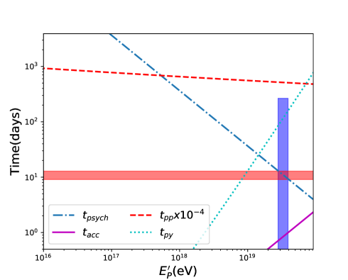
Figure 4: The blue dash-dot line depicts the proton synchrotron cooling time, the red dash line delineates the pp interaction time, and the blue shaded area marks the proton energy for which proton synchrotron cooling time between 8 to 12 days in the observer frame.

Table 3: The Parameters used in the lepto-hadronic model for the SEDs of 3C 279 quasar

Parameters	Values
z	$0.536$
d(Mpc)	$2.29\times 10^{3}$
$\delta$	$27$
$\Gamma_{j}$	$15$
B(G)	$2.3$
$R^{\prime}$ (cm)	$2\times 10^{16}$
$\alpha_{e}$	$1.8$
$\beta_{e}$	$.10$
${\gamma_{e,min}^{\prime}}$	${400}$
${\gamma_{e,max}^{\prime}}$	${1.2\times 10^{4}}$
$\alpha_{p}$	2.1
$\gamma_{p,min}^{\prime}$	$400$
$\gamma_{p}^{\prime b}$	$1.53\times 10^{10}$
$\gamma_{p,max}^{\prime}$	$4.4\times 10^{10}$
$L^{\prime}_{e}({erg}\;{s^{-1}})$	$3.92\times 10^{43}$
$L^{\prime}_{p}({erg}\;{s^{-1}})$	$1.56\times 10^{46}$
$T^{\prime}_{BLR}(K)$	$1.3\times{10}^{4}$
$U^{\prime}_{BLR(erg/cm^{3})}$	$9.67$
$T^{\prime}_{disk}(K)$	$2.3\times{10}^{6}$
$U^{\prime}_{disk}(erg/cm^{3})$	$7.\times{10}^{-7}$

III.3 VHE emissions with Proton Synchrotron :

The VHE activity events observed by H.E.S.S are explained here with the proton synchrotron emissions. The proton synchrotron photons starting from $E^{\prime}_{p}$ =$1.44\times 10{{}^{19}}$ eV till $E^{\prime}_{p,max}$ are calculated for magnetic field 2.3 G following [37, 19]. The synchrotron flux from a power-law proton spectrum is,

$$J(\nu)d\nu=A\;\nu^{-b}exp(-(\nu/\nu_{cut}))d\nu.$$ (3)

where A =$N_{0}/(48\;\pi^{2}d^{2})(\sigma_{T}\;m_{e}^{2}c/m_{p}^{2})(e/2\pi\;m_{p}c)^{(\alpha_{p}-3)/2}\\ \times(\delta/(1+z))^{(\alpha_{p}+5)/2}(B^{(\alpha_{p}+1)/2})$ , b =($\alpha_{p}$-1)/2 and $\nu_{cut}$ is obtained from equation 2.

IV Results & Discussion

The Fermi-LAT light curve of the quasar 3C 279 in the time period MJD 58131 to 58142 within the energy range 0.1 to 300 GeV suggests a flaring state in HE. However, the TeV gamma-ray with the H.E.S.S. telescope search indicates VHE activity with an 11-day delay from the peak of the HE flare. We explain both these events with a lepto-hadronic model. The lepton modeling to explain the SED events starting from UV wavelengths to HE events is shown in figure 3 with a solid (black) line, and the free parameters values of the model are listed in table 3. The synchrotron emissions from the accelerated protons explain the delayed VHE energy activity.

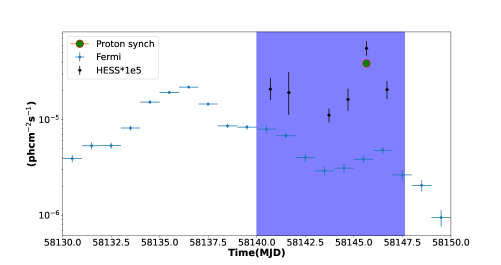
Figure 5: The light curve of FERMI-LAT analysis during the time period MJD 58130 to 58150 within the energy range 0.1 to 300 GeV. The cyan colour circles represent FERMI HE-$\gamma$ ray photon flux and black plus point for VHE activity observed by H.E.S.S during the time period MJD 58142 to 58150 and the red-green circle represents the integrated proton synchrotron emissions within the H.E.S.S energy limit.

We considered the accelerated protons to follow an exponential cutoff power law with index 2.1 (free parameter) within the energy range $\gamma^{\prime}_{p,min}$ ($=\gamma^{\prime}_{e}$) to $\gamma^{\prime}_{p,max}=4.4\times 10^{10}$. We calculated the value of $\gamma^{\prime}_{p,max}$ from equation 2 considering the highest energy events in H.E.S.S is at 500 GeV. The proton undergoes through p$\gamma$ interaction channel till energy $\frac{1}{t_{p\gamma}}=\frac{1}{t_{psych}}$, $\gamma_{b}^{p^{\prime}}=1.53\times 10^{10}$. We calculated the proton synchrotron emission from this energy till the $\gamma^{\prime}_{p,max}$ using equation 3. We explicitly show the proton synchrotron emission radiation in the magnetic field 2.3 G, in figure3 with dashed (magenta). We also show the VHE $\gamma$-ray emissions from the source after correction due to interaction with Extragalactic background light (EBL) with the dashed (red) line in the same figure. We calculated this suppression using for the source at a distance $d=2.29\times 10^{9}$ pc. The total proton luminosity is $L_{p}=1.56\times 10^{46}$ erg/sec. We show in figure 5 the integrated proton synchrotron emissions within the H.E.S.S energy limit in the light curve for the VHE activity with a filled circle (green). Note our hadron model explains the VHE activity within $2\sigma$.

Interestingly the counterpart neutrinos from the hadron model can give a smoking gun evidence of its robustness. The secondary neutrinos are produced through p$\gamma\rightarrow\pi^{\pm}X\rightarrow\mu^{\pm}\,\nu_{\mu}\,(\bar{\nu_{\mu}}),\mu^{\pm}\rightarrow\;e^{\pm}\;\nu_{e}(\bar{\nu_{e}}),\bar{\nu_{\mu}}(\nu_{\mu})$, where the $\gamma$’s are the BLR photons as discussed in section III.1. We calculated the muon type of neutrino flux using,

$${E^{2}_{\nu}}\frac{dN}{dE_{\nu}}=\frac{3}{4}min[1,f_{p\gamma}]{E^{2}_{p}}\frac{dN}{dE_{p}},$$ (4)

where the neutral and charged pion are produced with equal probability. $f_{{p\gamma}}=\frac{t*}{t_{p\gamma}}$ with $t*=16\,\text{days}$ being the model time period in the observer form and $t_{p\gamma}$ is calculated as shown in figure 4. We show the neutrino flux with dashed lines in figure 3. During the years 2012-2017, the IceCube neutrino observatory survey for point source resulted in a p-value of 19% for quasar 3C 279, which is compatible with the background [38]. An upper bound for this result is shown in figure 3.

An enhanced significant astrophysical observation encourages challenging theoretical interpretations of the high-energy astrophysical environment. We show one such observed event where there is a simultaneous survey report of nearly 11 days of delay in the VHE event from one of the extraordinary quasar, 3C 279. We explain this delay originated from a proton synchrotron channel compared to the historical model of electron IC. More multi-wavelength follow-observation would help in identifying the origin of VHE activities significantly.

V Acknowledgement

We would like to thank Foteini Oikonomou for her valuable suggestions, which improved the manuscript significantly. We would also like to acknowledge Abhradeep Roy for the discussions on data analysis. Sunanda would like to acknowledge the CSIR for providing a fellowship and fruitful discussion with Soebur Razzaque.

References

- IceCube Collaboration et al. [2018] IceCube Collaboration, M. G. Aartsen, M. Ackermann, J. Adams, J. A. Aguilar, M. Ahlers, and others, Science 361, 147 (2018), arXiv:1807.08794 [astro-ph.HE] .
- IceCube Collaboration et al. [2022] IceCube Collaboration, R. Abbasi, M. Ackermann, J. Adams, et al., Science 378, 538 (2022), arXiv:2211.09972 [astro-ph.HE] .
- Lynds et al. [1965] C. R. Lynds, A. N. Stockton, and W. C. Livingston, ApJ 142, 1667 (1965).
- MAGIC Collaboration et al. [2008] MAGIC Collaboration et al., Science 320, 1752 (2008), arXiv:0807.2822 [astro-ph] .
- Hartman et al. [1992] R. C. Hartman, D. L. Bertsch, et al., ApJ 385, L1 (1992).
- Paliya et al. [2015] V. S. Paliya, S. Sahayanathan, and C. S. Stalin, ApJ 803, 15 (2015), arXiv:1501.07363 [astro-ph.HE] .
- Hayashida et al. [2015] M. Hayashida, K. Nalewajko, G. M. Madejski, et al., ApJ 807, 79 (2015), arXiv:1502.04699 [astro-ph.HE] .
- Ackermann et al. [2016] M. Ackermann, R. Anantua, et al., ApJ 824, L20 (2016), arXiv:1605.05324 [astro-ph.HE] .
- Aleksić et al. [2011a] J. Aleksić, L. A. Antonelli, et al., ApJ 730, L8 (2011a), arXiv:1101.4645 [astro-ph.HE] .
- Aleksić et al. [2011b] J. Aleksić, L. A. Antonelli, P. Antoranz, M. Backes, J. A. Barrio, D. Bastieri, and others, A&A 530, A4 (2011b), arXiv:1101.2522 [astro-ph.CO] .
- Paliya [2015] V. S. Paliya, ApJ 808, L48 (2015), arXiv:1507.03073 [astro-ph.HE] .
- Böttcher et al. [2009] M. Böttcher, A. Reimer, and A. P. Marscher, ApJ 703, 1168 (2009).
- Petropoulou and Mastichiadis [2012] M. Petropoulou and A. Mastichiadis, MNRAS 426, 462 (2012), arXiv:1207.5227 [astro-ph.HE] .
- van Zyl et al. [2018] P. van Zyl, R. Ojha, et al., 11189 (2018).
- D’Ammando et al. [2018] F. D’Ammando, D. Fugazza, and S. Covino, The Astronomer’s Telegram 11190, 1 (2018).
- Lucarelli et al. [2018] F. Lucarelli, A. Bulgarelli, F. Verrecchia, et al., 11200 (2018).
- Xu et al. [2018] Z.-L. Xu, N.-H. Liao, K.-K. Duan, et al., 11246 (2018).
- de Naurois et al. [2018] M. de Naurois et al., 11239 (2018).
- Sunanda et al. [2022] Sunanda, R. Moharana, and P. Majumdar, Phys. Rev. D 106, 123005 (2022).
- Das et al. [2022] S. Das, N. Gupta, and S. Razzaque, A&A 668, A146 (2022), arXiv:2208.00838 [astro-ph.HE] .
- Prince [2020] R. Prince, ApJ 890, 164 (2020), arXiv:2001.04493 [astro-ph.HE] .
- Shah et al. [2019] Z. Shah, V. Jithesh, S. Sahayanathan, R. Misra, and N. Iqbal, MNRAS 484, 3168 (2019), arXiv:1901.04184 [astro-ph.HE] .
- Oberholzer and Böttcher [2019] L. L. Oberholzer and M. Böttcher, PoS HEASA2018, 024 (2019).
- Böttcher [2005] M. Böttcher, The Astrophysical Journal 621, 176 (2005).
- Kaur et al. [2018] A. Kaur, V. S. Paliya, M. Ajello, et al., 11202 (2018).
- Abdo et al. [2010] A. A. Abdo, M. Ackermann, M. Ajello, , and others, ApJ 722, 520 (2010), arXiv:1004.0348 [astro-ph.HE] .
- Akaike [1974] H. Akaike, IEEE Transactions on Automatic Control 19, 716 (1974).
- Dondi and Ghisellini [1995] L. Dondi and G. Ghisellini, Monthly Notices of the Royal Astronomical Society 273, 583 (1995), https://academic.oup.com/mnras/article-pdf/273/3/583/18539600/mnras273-0583.pdf .
- Ghisellini and Tavecchio [2009] G. Ghisellini and F. Tavecchio, MNRAS 397, 985 (2009), arXiv:0902.0793 [astro-ph.CO] .
- Pian et al. [1999] E. Pian, C. M. Urry, L. Maraschi, G. Madejski, I. M. McHardy, A. Koratkar, A. Treves, L. Chiappetti, P. Grandi, R. C. Hartman, H. Kubo, C. M. Leach, J. E. Pesce, C. Imhoff, R. Thompson, and A. E. Wehrle, The Astrophysical Journal 521, 112 (1999).
- Dermer et al. [2014] C. D. Dermer, M. Cerruti, B. Lott, C. Boisson, and A. Zech, ApJ 782, 82 (2014), arXiv:1304.6680 [astro-ph.HE] .
- Hahn [2016] J. Hahn, PoS ICRC2015, 917 (2016).
- Dermer and Menon [2009] C. D. Dermer and G. Menon, High Energy Radiation from Black Holes: Gamma Rays, Cosmic Rays, and Neutrinos (2009).
- Peterson [2006] B. M. Peterson, in Physics of Active Galactic Nuclei at all Scales, Vol. 693, edited by D. Alloin (2006) p. 77.
- Ptitsyna and Troitsky [2010] K. V. Ptitsyna and S. V. Troitsky, Physics Uspekhi 53, 691 (2010), arXiv:0808.0367 [astro-ph] .
- Nilsson et al. [2009] K. Nilsson, T. Pursimo, C. Villforth, E. Lindfors, and L. O. Takalo, A&A 505, 601 (2009), arXiv:0908.1618 [astro-ph.CO] .
- Aharonian [2002] F. A. Aharonian, MNRAS 332, 215 (2002), arXiv:astro-ph/0106037 [astro-ph] .
- Abbasi et al. [2021] R. Abbasi et al. (IceCube), Astrophys. J. 911, 67 (2021), arXiv:2012.01079 [astro-ph.HE] .