A theoretical view on the T-web statistical description of the cosmic web

Abstract

Context. The objective classification of the cosmic web into different environments is a striving field in large-scale structure studies both as a tool to study in more detail the formation of structures (halos and galaxies) and the link between their properties and the large-scale environment, and as another class of objects whose statistics contain cosmological information.

Aims. In this paper, we present an analytical framework to compute the probability of the different environments in the cosmic web based on the so-called T-web formalism that classifies structures in four different classes (voids, walls, filaments, and knots) by studying the eigenvalues of the Hessian of the gravitational potential, often called tidal tensor.

Methods. Our classification method relies on studying whether the eigenvalues of this Hessian matrix are below or above a given threshold and thus requires the knowledge of the joint probability distribution of those eigenvalues. In practice, we perform a change of variables in terms of rotational invariants that have the property to be polynomials of the field variables and minimally correlated. We study the distribution of those variables in the linear and quasi-linear regime with the help of a so-called Gram-Charlier expansion with tree-order Eulerian perturbation theory to compute the Gram-Charlier coefficients. This expansion then allows us to predict the probability of the four different environments as a function of the chosen threshold and at a given smoothing scale and redshift for the density field. We check the validity regime of our predictions by comparing those predictions to measurements made in the N-body Quijote simulations.

Results. Working with fields normalized by their linear variance, we find that scaling the threshold value with the non-linear amplitude of fluctuations allows us to capture almost entirely the redshift evolution of the probability of the four environments, even if we assume that the density field is Gaussian (corresponding to the linear regime of structure formation). We also show that adding mild non-Gaussian corrections with the help of a Gram-Charlier expansion – hence introducing corrections that depend on third-order cumulants of the field – provides even greater accuracy allowing us to obtain very precise predictions for cosmic web abundances up to scales as small as $\sim$ 5 Mpc/h and redshifts down to z $\sim$ 0.

1 Introduction

It is a well-known fact that the large-scale distribution of matter throughout the Universe is well-approximated by a filamentary structure dubbed the cosmic web (de Lapparent et al. 1986). From a theoretical point of view, the first building blocks for a description of the cosmic web goes back to the seminal work of Zel’dovich (1970) and many other that followed e.g. Arnold et al. (1982) or Klypin & Shandarin (1983). Indeed, the so-called Zeldovich approximation – describing the first-order ballistic trajectories of particles in a Lagrangian description – predicts the existence of ”pancakes” (i.e. sheet-like tenuous walls), filaments, and clusters due to the collapse of anisotropic primordial fluctuations through gravitational instabilities in our expanding Universe. In the 90s, Bond et al. (1996); Klypin & Shandarin (1983) showed that this ensemble of objects forms a connected network called the cosmic web due to the correlations imprinted in the primordial fluctuations. Initial peaks led to the formation of clusters at the nodes of the web while initial correlation bridges in between later form filaments that lie within walls which themselves surround nearly empty void regions. Such a web classification can be achieved through the eigenvalues of the linear deformation tensor, namely stating that if all eigenvalues are negative (or below a threshold that is here taken to zero) then the region is expanding in 3D thus describing a void region; if all values are positive then the region is contracting thus describing a knot, and where the other two configurations of eigenvalues lead to either walls or filaments.

Another classification method was later introduced in Hahn et al. (2007a), Aragón-Calvo et al. (2007a) and Forero-Romero et al. (2009) using tidal fields, that is evaluating the Hessian of the gravitational potential, either theoretically in the linear regime or the non-linear potential estimated in dark-matter only numerical simulations. In the following years, several works have developed different classification schemes, to improve the detection of these cosmic web structures in various types of data (continuous fields, simulated datasets, point-like galaxy surveys, etc). For instance, Aragón-Calvo et al. (2010a) used the SpineWeb framework to segment the density field, Falck et al. (2012) showed how to classify morphological structures using the ORIGAMI method i.e. counting the number of orthogonal folds in the Lagrangian phase space sheet, and various authors have applied techniques from (continuous then discrete) Morse theory (Colombi et al. 2000) to identify topological structures in the cosmological density field (Sousbie et al. 2008; Aragón-Calvo et al. 2007a; Sousbie et al. 2009; Sousbie 2011). Alternatively, Hoffman et al. (2012) introduced the V-web classification scheme this time based on the shear of the velocity field and showing that it is able to better resolve smaller structures which in turn allows for studying finer dark-matter halos properties. An extension of this idea to Lagrangian settings was later proposed by Fisher et al. (2016). Note that the velocity and density fields are closely related (for example through the mass-conservation equation in the Vlasov-Poisson system) and their statistics are virtually equivalent in the linear regime of structure formation. We refer the readers to Wang et al. (2014); Wang & Szalay (2014) for a thorough investigation of the differences between the dynamical and kinematical classifications.

Beyond the strict motivation of wanting to describe the cosmic web from a mathematical point of view, the classification schemes allow us to explore many different environmental effects on the properties of dark-matter halos (Hahn et al. 2007a, b; Aragón-Calvo et al. 2007b, 2010b; Codis et al. 2012; Libeskind et al. 2013) and galaxies within them (Nuza et al. 2014; Metuki et al. 2015; Poudel et al. 2017; Kraljic et al. 2018; Codis et al. 2018a; Hasan et al. 2023). The cosmic web classification is also a smoking gun for discriminating between cosmological models as shown for instance by Lee & Park (2009) using voids specifically, Codis et al. (2013) with counts of cosmic web critical points, Codis et al. (2018b) using the connectivity of the filaments or Bonnaire et al. (2022) relying on the power spectrum of the various cosmic web environments. Understanding how this cosmic web evolves with time and scale is hence paramount both for cosmology and galaxy formation that takes place within this large-scale environment. This evolution has been studied theoretically in some contexts like the local skeleton Pogosyan et al. (2009) and on various numerical works. One such example is the recent work by Cui et al. (2017, 2019) which investigated in simulations the abundances of the various environments and their time evolution relying on the T and V-web decompositions. However, no theoretical model based on first principles has been explicitly derived so far to our knowledge while this is at reach of standard techniques used in large-scale structure theoretical studies.

In this paper, we hence propose to derive theoretical predictions for web classifications defined by means of the T-web definition. We will first focus on a Gaussian description of the cosmic density field before turning to mild non-Gaussian corrections.

To assess the validity regime of our theoretical formalism and predictions for the one-point statistics of all four cosmic environments, we compare our results with measurements made in a dark-matter-only N-body numerical simulation, the Quijote simulation (Villaescusa-Navarro et al. 2020). Their simulated box has a size of $1$ Gpc/h, with $1024^{3}$ dark matter particles. We are using their high-resolution, fiducial cosmology, snapshots at 5 different redshifts: $z=0,0.5,1,2,3$. Their fiducial cosmology is {$\Omega_{m},\leavevmode\nobreak\ \Omega_{b},\leavevmode\nobreak\ h,\leavevmode\nobreak\ n_{s},\sigma_{8}$} = {$0.3175,\leavevmode\nobreak\ 0.049,\leavevmode\nobreak\ 0.6711,\leavevmode\nobreak\ 0.9624,\leavevmode\nobreak\ 0.834$}. Finally, for better statistical relevance, we typically average our measurements over 11 realizations of the Quijote suite and use those realizations to estimate error bars.

The outline of the paper is as follows. We first describe the T-web and V-web classifications in section 2. We then present in section 3 the theoretical formalism and the predictions obtained for the probability of the different environments (as a function of a threshold, redshift, and smoothing scale) in the linear regime of structure formation, that is assuming a Gaussian matter density field. Section 4 introduces a Gram-Charlier expansion to include non-Gaussian (i.e. non-linear) corrections to the joint-PDF of the elements of the Hessian of the gravitational potential, and we finally discuss and conclude on our results in section 5.

2 T-web classification of the cosmic web

Among many possibilities (Libeskind et al. 2017), one commonly used mathematical way to classify the different cosmological environments is based on the number of eigenvalues of a deformation tensor above a threshold. Several definitions can be used for this deformation tensor (strain tensor, mass tensor, etc.) but the classification can always follow this outline:

• 0 eigenvalue above the threshold: void,

• 1 eigenvalue above the threshold: wall,

• 2 eigenvalues above the threshold: filament,

• 3 eigenvalues above the threshold: knot.

Notably, the T-web classification developed by Forero-Romero et al. (2009) is based on the tidal shear tensor $T$ which is the tensor of the second derivative of the gravitational potential

$$T_{ij}=\frac{\partial^{2}\Phi}{\partial r_{i}r_{j}},$$ (1)

where $\Phi$ is the gravitational potential and $r_{i}$ with $i=1,2,3$ the spatial coordinates. Alternatively, the V-web classification developed by Hoffman et al. (2012) is based on the velocity shear tensor $\Sigma$

$$\Sigma_{ij}=-\frac{1}{2}\left(\frac{\partial v_{i}}{\partial r_{j}}+\frac{\partial v_{j}}{\partial r_{i}}\right)/H_{0},$$ (2)

where $H_{0}$ is the Hubble constant and $v$ the velocity. Note that both of the above classifications are similar to the one used by Hahn et al. (2007a). Given those definitions, in practice, one can start from field maps, compute the deformation tensor, diagonalize it, and obtain the number of eigenvalues above a given threshold $\Lambda_{\text{th}}$ at each spatial position, thus dividing the cosmic web into four characteristic classes.

Usually, the value of this threshold is not fixed a priori in the literature and is often chosen in order to obtain a satisfactory visual agreement between the log density field and the classification. Originally, Hahn et al. (2007a) took $\Lambda_{\text{th}}=0$ to distinguish structures with inner or outer flows. Follow-up studies demonstrated that having a non-zero threshold leads to a better visual match (for example, Forero-Romero et al. 2009; Libeskind et al. 2017; Suárez-Pérez et al. 2021; Cui et al. 2017; Hoffman et al. 2012; Carlesi et al. 2014). The threshold is generally taken as a positive constant, between $0$ and $1$, and usually does not depend on the redshift or smoothing scale but note that a positive threshold will tend to underline the most extreme knots and filaments (which is usually what is meant by good visual agreement) while a negative threshold would then underline the most empty voids.

In the remainder of the paper, we will focus on the T-web formalism, although we emphasize that the V-web description would yield identical results at first perturbative order in a Lagrangian framework (the so-called 1LPT or Zeldovitch approximation). This is indeed due to the usual expression for these ballistic trajectories where the velocity is given by the gradient of the gravitational potential up to a uniform time-dependent factor (Zel’dovich 1970). As an example of the accuracy of this classification scheme, we present in figure 1 a comparison of the density contrast (first and third columns, with a continuous color bar) at different redshifts and smoothing scales, with the classification obtained using the T-web (second and fourth column, with a discrete color bar) at the same redshifts and smoothing scales. In the second and fourth columns, voids are shown in dark blue, walls in blue, filaments in green, and nodes in red. As expected from the T-web classification, we obtain the environments of the simulation by computing the second derivative of the potential and looking at the number of eigenvalues above our chosen threshold. Here, we are using a threshold $\Lambda_{\text{t}h}=0.01$ for every redshift and smoothing scale, based on the value used in Cui et al. (2017), chosen to have a good visual agreement. For instance, the knots and voids (respectively in red and dark blue) can easily be identified by eye in both visualizations and are at the same position as rare maxima and minima in the density contrast maps.

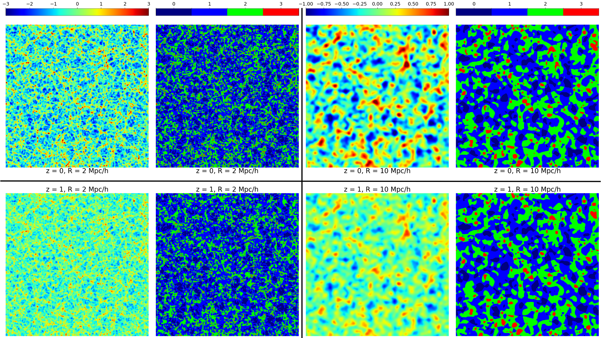
Figure 1: Logarithm of the density contrast of one slice of height and width $1$ Gpc/h and  $2$ Mpc/h in thickness of the Quijote simulation (first and third column) compared with the classification obtained using the T-web (second and fourth column) at different redshifts and smoothing scales. For the T-web classification, the color bar is the number of eigenvalues above our chosen threshold $\Lambda_{\text{th}}$ = 0.01 chosen specifically for good visual agreement.

To build a theoretical description of the cosmic web as defined by the T-web description, let us first define the variance of the contrast of the density field, $\delta=(\rho-\langle\rho\rangle)/\langle\rho\rangle$,

$$\sigma_{0}^{2}=\langle\delta^{2}\rangle.$$ (3)

Following Pogosyan et al. (2009), we choose to normalize the derivatives of the gravitational potential by their variance such that

$$\nu=\frac{1}{\sigma_{0}}\delta,\qquad\phi_{ij}=\frac{1}{\sigma_{0}}\nabla_{i}\nabla_{j}\Phi.$$ (4)

Formally given our classification method, the probability of each cosmic environment then depends on the joint probability distribution ${\cal P}$ of the eigenvalues of the tidal tensor. Given our normalization choice in equations (4), we use here the eigenvalues normalized by their variance (or equivalently the eigenvalues of the normalized tidal tensor) that we denote $\lambda_{1}\leq\lambda_{2}\leq\lambda_{3}$. The probability of the four environments then reads

$$P_{\text{void}}=\int{\rm d}\lambda_{1}{\rm d}\lambda_{2}{\rm d}\lambda_{3}\;{\cal P}(\lambda_{1},\lambda_{2},\lambda_{3})Boole(\lambda_{1}<\lambda_{2}<\lambda_{3}<\lambda_{\rm th})$$ (5)

$$P_{\text{wall}}=\int{\rm d}\lambda_{1}{\rm d}\lambda_{2}{\rm d}\lambda_{3}\;{\cal P}(\lambda_{1},\lambda_{2},\lambda_{3})Boole(\lambda_{1}<\lambda_{2}<\lambda_{\rm th}<\lambda_{3}),$$ (6)

$$P_{\text{filament}}=\int{\rm d}\lambda_{1}{\rm d}\lambda_{2}{\rm d}\lambda_{3}\;{\cal P}(\lambda_{1},\lambda_{2},\lambda_{3})Boole(\lambda_{1}<\lambda_{\rm th}<\lambda_{2}<\lambda_{3}),$$ (7)

$$P_{\text{knot}}=\int{\rm d}\lambda_{1}{\rm d}\lambda_{2}{\rm d}\lambda_{3}\;{\cal P}(\lambda_{1},\lambda_{2},\lambda_{3})Boole(\lambda_{\rm th}<\lambda_{1}<\lambda_{2}<\lambda_{3}),$$ (8)

where $\{\lambda_{i}\}_{i=1,2,3}$ are the orderly eigenvalues of the $(\phi_{ij})_{1\leq i,j\leq 3}$ matrix and $Boole$ is a Boolean equal to 1 if the condition is satisfied, 0 otherwise.

As we are now working with normalized eigenvalues, and keeping our earlier choice of a $\Lambda_{\rm th}=0.01$ value, our threshold will be given by $\lambda_{\rm th}={(\Lambda_{\rm th}=0.01)}/{\sigma(z)}$, with

$$\sigma^{2}(z)=4\pi\int{\rm d}k\,k^{2}P(k,z)W(kR)^{2},$$ (9)

where $W(kR)$ is the applied smoothing which in this paper will be Gaussian with a smoothing scale $R$ such that

$$W_{\text{G}}(kR)=\exp\left(-\frac{1}{2}k^{2}R^{2}\right),$$ (10)

and $P(k,z)$ is the matter density power spectrum. We denote the linear variance $\sigma_{0}^{2}$ when using the linear power spectrum, which is computed using the Boltzmann code Camb (Lewis et al. 2000), and $\sigma_{\text{NL}}^{2}$ the non-linear variance (for instance measured in the simulation).

3 Cosmic web abundances in the linear regime

To obtain some theoretical intuition of the probability of the different cosmic environments in the density field and their redshift evolution, let us first consider the density field at linear order in Eulerian perturbation theory i.e. let us assume that it is Gaussian. For a Gaussian density field, the associated gravitational potential and its successive derivatives are also Gaussian-distributed so that we can use the Doroshkevich formula (Doroshkevich 1970) which gives the joint probability distribution of eigenvalues of a Gaussian symmetric matrix

$${\cal P}_{D}(\lambda_{1},\lambda_{2},\lambda_{3})=\frac{675\sqrt{5}e^{\frac{3}{4}(\lambda_{1}+\lambda_{2}+\lambda_{3})^{2}-\frac{15}{4}(\lambda_{1}^{2}+\lambda_{2}^{3}+\lambda_{3}^{2})}}{8\pi}(\lambda_{3}-\lambda_{2})(\lambda_{2}-\lambda_{1})(\lambda_{3}-\lambda_{1}).$$ (11)

Note that the general expression for the multi-dimensional PDF of the tidal tensor in Cartesian coordinates $X=\{\phi_{ij}\}$ in the Gaussian case reads

$${\cal P_{G}}(X)=(2\pi)^{-N/2}|C|^{-1/2}\exp\left(-\frac{1}{2}XC^{-1}X\right),$$ (12)

where $C$ is its covariance matrix.

From equation (11), we can then numerically integrate equations (5)-(8) to obtain the probability of the various environments. In practice, those 3D integrals can actually be reduced to 1D as two degrees of freedom can be analytically integrated out. For that purpose, one needs to express the three degrees of freedom of the tidal tensor that are rotationally invariant as polynomials of its Cartesian coordinates $\phi_{ij}$ (in contrast to eigenvalues that are not). Following for instance Pogosyan et al. (2009), a natural option can be the three coefficients of its characteristic polynomial

$$I_{1} = Tr(\phi_{ij})=\phi_{11}+\phi_{22}+\phi_{33}=\lambda_{1}+\lambda_{2}+\lambda_{3}=\nu,$$ (13)

$$I_{2} = \phi_{11}\phi_{22}+\phi_{22}\phi_{33}+\phi_{11}\phi_{33}-\phi_{12}^{2}-\phi_{23}^{2}-\phi_{13}^{2}=\lambda_{1}\lambda_{2}+\lambda_{2}\lambda_{3}+\lambda_{1}\lambda_{3},$$ (14)

$$I_{3} = det|\phi_{ij}|=\phi_{11}\phi_{22}\phi_{33}+2\phi_{12}\phi_{23}\phi_{13}-\phi_{11}\phi_{23}^{2}-\phi_{22}\phi_{13}^{2}-\phi_{33}\phi_{12}^{2}=\lambda_{1}\lambda_{2}\lambda_{3}.$$ (15)

To get variables that are as uncorrelated as possible, a simplification proposed by Pogosyan et al. (2009) is to use combinations of the $\{I_{k}\}_{1\geq k\geq 3}$ that will be denoted $\{J_{k}\}_{1\geq k\geq 3}$ such that the first variable is again the trace of the tidal tensor but higher order variables only depends on the trace-less part of that tensor and are thus uncorrelated with the trace in the Gaussian case. After some algebra, one can easily find

$$J_{1}=I_{1},\qquad J_{2}=I_{1}^{2}-3I_{2},\qquad J_{3}=I_{1}^{3}-\frac{9}{2}I_{1}I_{2}+\frac{27}{2}I_{3}.$$ (16)

For a Gaussian random field, one can easily show that the probability distribution function of the above-defined variables reads (Pogosyan et al. 2009)

$${\cal P_{G}}(J_{1},J_{2},J_{3})=\frac{25\sqrt{5}}{12\pi}\exp\left[-\frac{1}{2}J_{1}^{2}-\frac{5}{2}J_{2}\right].$$ (17)

where $J_{2}\geq 0$ and $J_{3}$ is uniformly distributed between its boundaries such that $-J_{2}^{3/2}\leq J_{3}\leq{J_{2}^{3/2}}$. Let us note that the probability distribution of J’s can be easily mapped to the Doroskevitch formula for the distribution of the eigenvalues after taking into account the usual Vandermonde determinant.

To get the probabilities for the different environments, we use a criterion on the number of eigenvalues superior to the threshold. As we are now working with variables $(J_{1},J_{2},J_{3})$, we have to translate the criterion on eigenvalues into this new set of variables. Following Pogosyan et al. (2009); Gay et al. (2012), we can obtain the integration limits for the four different environments as follows

$$P_{\text{void}} = \int_{0}^{\infty}{\rm d}J_{2}\int_{-\infty}^{-2\sqrt{J_{2}}+3\lambda_{\rm th}}{\rm d}J_{1}\int_{-J_{2}^{3/2}}^{J_{2}^{3/2}}{\rm d}J_{3}\,{\cal P_{G}}(J_{1},J_{2},J_{3})+\int_{0}^{\infty}{\rm d}J_{2}\int_{-2\sqrt{J_{2}}+3\lambda_{\rm th}}^{-\sqrt{J_{2}}+3\lambda_{\rm th}}\!\!\!\!\!{\rm d}J_{1}\int_{-J_{2}^{3/2}}^{-\frac{1}{2}(J_{1}-3\lambda_{\rm th})^{3}+\frac{3}{2}(J_{1}-3\lambda_{\rm th})J_{2}}\!\!\!\!\!\!\!\!\!\!\!\!\!\!\!\!\!\!\!\!\!\!\!\!\!\!\!\!\!\!\!\!\!\!\!\!\!\!\!\!\!\!{\rm d}J_{3}{\cal P_{G}}(J_{1},J_{2},J_{3}),$$ (18)

$$P_{\text{wall}} = \int_{0}^{\infty}{\rm d}J_{2}\int_{-2\sqrt{J_{2}}+3\lambda_{\rm th}}^{\sqrt{J_{2}}+3\lambda_{\rm th}}{\rm d}J_{1}\int_{-\frac{1}{2}(J_{1}-3\lambda_{\rm th})^{3}+\frac{3}{2}(J_{1}-3\lambda_{\rm th})J_{2}}^{J_{2}^{3/2}}\!\!\!\!\!\!\!\!\!\!\!\!\!\!\!\!\!\!\!\!\!\!\!\!\!\!\!\!\!\!\!\!\!\!\!\!\!{\rm d}J_{3}{\cal P_{G}}(J_{1},J_{2},J_{3}),$$ (19)

$$P_{\text{filament}} = \int_{0}^{\infty}{\rm d}J_{2}\int_{-\sqrt{J_{2}}+3\lambda_{\rm th}}^{2\sqrt{J_{2}}+3\lambda_{\rm th}}{\rm d}J_{1}\int_{-J_{2}^{3/2}}^{-\frac{1}{2}(J_{1}-3\lambda_{\rm th})^{3}+\frac{3}{2}(J_{1}-3\lambda_{\rm th})J_{2}}\!\!\!\!\!\!\!\!\!\!\!\!\!\!\!\!\!\!\!\!\!\!\!\!\!\!\!\!\!\!\!\!\!\!\!\!\!{\rm d}J_{3}{\cal P_{G}}(J_{1},J_{2},J_{3}),$$ (20)

$$P_{\text{knot}} = \int_{0}^{\infty}{\rm d}J_{2}\int_{\sqrt{J_{2}}+3\lambda_{\rm th}}^{2\sqrt{J_{2}}+3\lambda_{\rm th}}{\rm d}J_{1}\int_{-\frac{1}{2}(J_{1}-3\lambda_{\rm th})^{3}+\frac{3}{2}(J_{1}-3\lambda_{\rm th})J_{2}}^{J_{2}^{3/2}}\!\!\!\!\!\!\!\!\!\!\!\!\!\!\!\!\!\!\!\!\!\!\!\!\!\!\!\!\!\!\!\!\!\!\!\!\!{\rm d}J_{3}{\cal P_{G}}(J_{1},J_{2},J_{3})+\int_{0}^{\infty}{\rm d}J_{2}\int_{2\sqrt{J_{2}}+3\lambda_{\rm th}}^{\infty}{\rm d}J_{1}\int_{-J_{2}^{3/2}}^{J_{2}^{3/2}}{\rm d}J_{3}{\cal P_{G}}(J_{1},J_{2},J_{3}).$$ (21)

The analytical integration over $J_{1}$ and $J_{3}$ can now be performed and we thus obtain the following probability of the four environments (written in terms of 1D integrals over $J_{2}$)

$$\begin{split}P_{\text{void}}&=\int_{0}^{\infty}\frac{25\sqrt{5}}{48\pi}e^{-\frac{5J_{2}}{2}}\Biggl{[}-\sqrt{2\pi}\bigl{(}2J_{2}^{3/2}-9J_{2}\text{$\lambda_{\rm th}$}+9\left(3\text{$\lambda_{\rm th}$}^{3}+\text{$\lambda_{\rm th}$}\right)\bigr{)}\text{erf}\left(\frac{3\text{$\lambda_{\rm th}$}-2\sqrt{J_{2}}}{\sqrt{2}}\right)\\ &+\sqrt{2\pi}\left(2J_{2}^{3/2}-9J_{2}\text{$\lambda_{\rm th}$}+9\left(3\text{$\lambda_{\rm th}$}^{3}+\text{$\lambda_{\rm th}$}\right)\right)\text{erf}\left(\frac{3\text{$\lambda_{\rm th}$}-\sqrt{J_{2}}}{\sqrt{2}}\right)+4\sqrt{2\pi}J_{2}^{3/2}\text{erfc}\left(\frac{2\sqrt{J_{2}}-3\text{$\lambda_{\rm th}$}}{\sqrt{2}}\right)\\ &-2e^{-\frac{1}{2}\left(2\sqrt{J_{2}}-3\text{$\lambda_{\rm th}$}\right)^{2}}\left(6\sqrt{J_{2}}\text{$\lambda_{\rm th}$}+J_{2}+9\text{$\lambda_{\rm th}$}^{2}+2\right)+e^{-\frac{1}{2}\left(\sqrt{J_{2}}-3\text{$\lambda_{\rm th}$}\right)^{2}}\left(6\sqrt{J_{2}}\text{$\lambda_{\rm th}$}-4J_{2}+18\text{$\lambda_{\rm th}$}^{2}+4\right)\Biggr{]}{\rm d}J_{2},\end{split}$$ (22)

 

$$\begin{split}P_{\text{wall}}&=\int_{0}^{\infty}\frac{25\sqrt{5}}{48\pi}e^{-\frac{5J_{2}}{2}}\Biggl{[}-\sqrt{2\pi}(2J_{2}^{3/2}+9J_{2}\text{$\lambda_{\rm th}$}-9\left(3\text{$\lambda_{\rm th}$}^{3}+\text{$\lambda_{\rm th}$}\right))\text{erf}\left(\frac{3\text{$\lambda_{\rm th}$}-2\sqrt{J_{2}}}{\sqrt{2}}\right)\\ &+\sqrt{2\pi}\left(2J_{2}^{3/2}+9J_{2}\text{$\lambda_{\rm th}$}-9\left(3\text{$\lambda_{\rm th}$}^{3}+\text{$\lambda_{\rm th}$}\right)\right)\text{erf}\left(\frac{\sqrt{J_{2}}+3\text{$\lambda_{\rm th}$}}{\sqrt{2}}\right)+2e^{-\frac{1}{2}\left(2\sqrt{J_{2}}-3\text{$\lambda_{\rm th}$}\right)^{2}}\left(6\sqrt{J_{2}}\text{$\lambda_{\rm th}$}+J_{2}+9\text{$\lambda_{\rm th}$}^{2}+2\right)\\ &+2e^{-\frac{1}{2}\left(\sqrt{J_{2}}+3\text{$\lambda_{\rm th}$}\right)^{2}}\left(3\sqrt{J_{2}}\text{$\lambda_{\rm th}$}+2J_{2}-9\text{$\lambda_{\rm th}$}^{2}-2\right)\Biggr{]}{\rm d}J_{2},\end{split}$$ (23)

 

$$\begin{split}P_{\text{filament}}&=\int_{0}^{\infty}-\frac{25\sqrt{5}}{48\pi}e^{-\frac{5J_{2}}{2}}\Biggl{[}-\sqrt{2\pi}(2J_{2}^{3/2}-9J_{2}\text{$\lambda_{\rm th}$}+9\left(3\text{$\lambda_{\rm th}$}^{3}+\text{$\lambda_{\rm th}$}\right))\text{erf}\left(\frac{2\sqrt{J_{2}}+3\text{$\lambda_{\rm th}$}}{\sqrt{2}}\right)\\ &+\sqrt{2\pi}\left(2J_{2}^{3/2}-9J_{2}\text{$\lambda_{\rm th}$}+9\left(3\text{$\lambda_{\rm th}$}^{3}+\text{$\lambda_{\rm th}$}\right)\right)\text{erf}\left(\frac{3\text{$\lambda_{\rm th}$}-\sqrt{J_{2}}}{\sqrt{2}}\right)-2e^{-\frac{1}{2}\left(2\sqrt{J_{2}}+3\text{$\lambda_{\rm th}$}\right)^{2}}\left(-6\sqrt{J_{2}}\text{$\lambda_{\rm th}$}+J_{2}+9\text{$\lambda_{\rm th}$}^{2}+2\right)\\ &+e^{-\frac{1}{2}\left(\sqrt{J_{2}}-3\text{$\lambda_{\rm th}$}\right)^{2}}\left(6\sqrt{J_{2}}\text{$\lambda_{\rm th}$}-4J_{2}+18\text{$\lambda_{\rm th}$}^{2}+4\right)\Biggr{]}{\rm d}J_{2},\end{split}$$ (24)

 

$$\begin{split}P_{\text{knot}}&=\int_{0}^{\infty}\frac{25\sqrt{5}}{48\pi}e^{-\frac{5J_{2}}{2}}\Biggl{[}-\sqrt{2\pi}(2J_{2}^{3/2}+9J_{2}\text{$\lambda_{\rm th}$}-9\left(3\text{$\lambda_{\rm th}$}^{3}+\text{$\lambda_{\rm th}$}\right))\text{erf}\left(\frac{\sqrt{J_{2}}+3\text{$\lambda_{\rm th}$}}{\sqrt{2}}\right)\\ &+\sqrt{2\pi}\left(2J_{2}^{3/2}+9J_{2}\text{$\lambda_{\rm th}$}-9\left(3\text{$\lambda_{\rm th}$}^{3}+\text{$\lambda_{\rm th}$}\right)\right)\text{erf}\left(\frac{2\sqrt{J_{2}}+3\text{$\lambda_{\rm th}$}}{\sqrt{2}}\right)+4\sqrt{2\pi}J_{2}^{3/2}\text{erfc}\left(\frac{2\sqrt{J_{2}}+3\text{$\lambda_{\rm th}$}}{\sqrt{2}}\right)\\ &-2e^{-\frac{1}{2}\left(2\sqrt{J_{2}}+3\text{$\lambda_{\rm th}$}\right)^{2}}\left(-6\sqrt{J_{2}}\text{$\lambda_{\rm th}$}+J_{2}+9\text{$\lambda_{\rm th}$}^{2}+2\right)+e^{-\frac{1}{2}\left(\sqrt{J_{2}}+3\text{$\lambda_{\rm th}$}\right)^{2}}\left(-6\sqrt{J_{2}}\text{$\lambda_{\rm th}$}-4J_{2}+18\text{$\lambda_{\rm th}$}^{2}+4\right)\Biggr{]}{\rm d}J_{2},\end{split}$$ (25)

where $\text{erf}(z)$ is the error function $\text{erf}(z)={2}\int_{0}^{z}e^{-t^{2}}dt/{\sqrt{\pi}}$ and $\text{erfc}(z)$ is the complementary error function $\text{erfc}(z)=1-\text{erf}(z).$

It is then possible to perform numerical integrations and obtain the probability of each environment. This is illustrated in figure 2, where the probability of the different environments as a function of redshift is shown. Each panel corresponds to a different Gaussian smoothing scale and displays the probability of voids, walls, filaments, and knots respectively in blue, green, yellow, and red. The dots are the measurements obtained from the simulation, the dashed lines represent the Gaussian prediction obtained with the formalism described in this section, and the solid lines – which can be ignored for now – are the predictions at next-to-leading order obtained with a Gram-Charlier expansion described in section 4 below. As expected, we observe that the higher the redshift and/or the larger the smoothing scale – and thus the closer the simulation gets to the linear regime –, the closer the Gaussian prediction to the measurements. At lower redshift and smaller smoothing scales, non-Gaussianities are more important and departures from the Gaussian prediction thus appear. Here, all probabilities are computed using a threshold $\lambda_{\rm th}={0.01}/{\sigma_{\text{NL}}}$ inspired from the literature (using simulations) for which the evolution of $\sigma$ with redshift and smoothing scale is given in Table 1. Note that the variance used solely in the normalization of the threshold is the non-linear variance measured from the simulation. This allows us to have a meaningful threshold – in terms of rarity – even though we describe the cosmic structures in linear theory. Given the good agreement with the simulation already with a Gaussian theory for large enough scale and redshift, this states that the probability of environments is roughly captured by the statistics of a Gaussian field, at least for redshifts and scales that typically correspond to typical variances $\sigma\lesssim 0.1$. Consequently, the redshift evolutions seen in previous works (Cui et al. 2017, 2019) with a fixed threshold can be roughly understood simply as the non-linear evolution of the amplitude of fluctuations for that threshold. This is because a fixed threshold in non-linear densities does not correspond to a fixed ”rarity” or ”abundance” threshold for which the cosmic evolution would be much less important. This interpretation is notably valid for large enough scale and redshift. Beyond $\sigma\sim 0.1$, such a Gaussian field approximation starts to break down. In the next section, we will see how one can improve the accuracy of the theoretical model with the help of Gram-Charlier corrections.

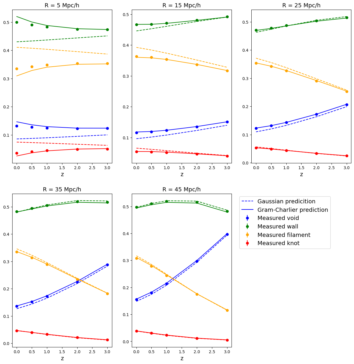
Figure 2: Probabilities of voids, walls, filaments, and knots respectively in blue, green, orange, and red, as a function of the redshift. Each panel is obtained at a given smoothing scale. Dots are measurements from the simulation, dashed lines are the Gaussian prediction and solid lines are the prediction obtained with the Gram-Charlier formalism at next-to-leading order. The error bars are errors on the mean but are too small to be distinguished.

Table 1: Standard deviation at different redshifts and (Gaussian) smoothing scales. The first value is the measurement from the Quijote simulation $\sigma_{\text{NL}}$, while the second column in parenthesis is the linear prediction $\sigma_{0}$.

z / R (Mpc/h)	$5$	$15$	$25$	$35$	$45$	$55$	$65$
$0$	$0.71$ ($0.68$)	$0.26$ ($0.26$)	$0.15$ ($0.15$)	$0.10$ ($0.10$)	$0.074$ ($0.072$)	$0.057$ ($0.055$)	$0.045$ ($0.043$)
$0.5$	$0.54$ ($0.52$)	$0.20$ ($0.20$)	$0.12$ ($0.12$)	$0.078$ ($0.077$)	$0.57$ ($0.056$)	$0.044$ ($0.042$)	$0.34$ ($0.033$)
$1$	$0.42$ ($0.41$)	$0.16$ ($0.16$)	$0.091$ ($0.091$)	$0.061$ ($0.061$)	$0.045$ ($0.044$)	$0.034$ ($0.033$)	$0.027$ ($0.026$)
$2$	$0.29$ ($0.28$)	$0.11$ ($0.11$)	$0.063$ ($0.062$)	$0.042$ ($0.042$)	$0.031$ ($0.030$)	$0.024$ ($0.023$)	$0.019$ ($0.018$)
$3$	$0.21$ ($0.22$)	$0.082$ ($0.082$)	$0.047$ ($0.047$)	$0.032$ ($0.031$)	$0.023$ ($0.023$)	$0.018$ ($0.017$)	$0.014$ ($0.014$)

Before turning to the case of non-Gaussian corrections, let us emphasize that our Gaussian theoretical formalism allows us to obtain the probability of voids, walls, filaments, and knots as a function of the threshold itself as illustrated in figure 3 for redshift $z=0$ and Gaussian smoothing R $=15$ Mpc/h. The threshold used in our previous analysis is the vertical black dashed line. For that choice of a mildly non-linear regime and for all the environments, we can draw the same conclusion as before: the qualitative picture is correctly captured but non-linear corrections are nonetheless necessary to improve the predictive power of our model. This figure could be helpful to guide the choice of the threshold from theoretical arguments. Note that an alternative approach could be to renounce defining a global threshold and choose it according to the studied environment(s). For example, one could determine the threshold that gives the 20% rarest knots and using the same threshold for the filaments, and similarly obtaining a threshold for the voids and walls (that would be the opposite of the previous one in the simple Gaussian case). In this case, some spatial position may be in none of the environments and this will mean that this position is a transition between two environments. Another possibility would be to use the filling factor approach to fix a threshold in abundance (i.e we fix the volume fraction occupied by the excursion above $\nu$ (Gott et al. 1987; Matsubara 2003), this would lead to a remapping of our environments.

Hereafter, we stick to the standard global-threshold strategy. The description and inclusion of the above-mentioned non-linear theoretical corrections are now the goals of the remainder of this paper.

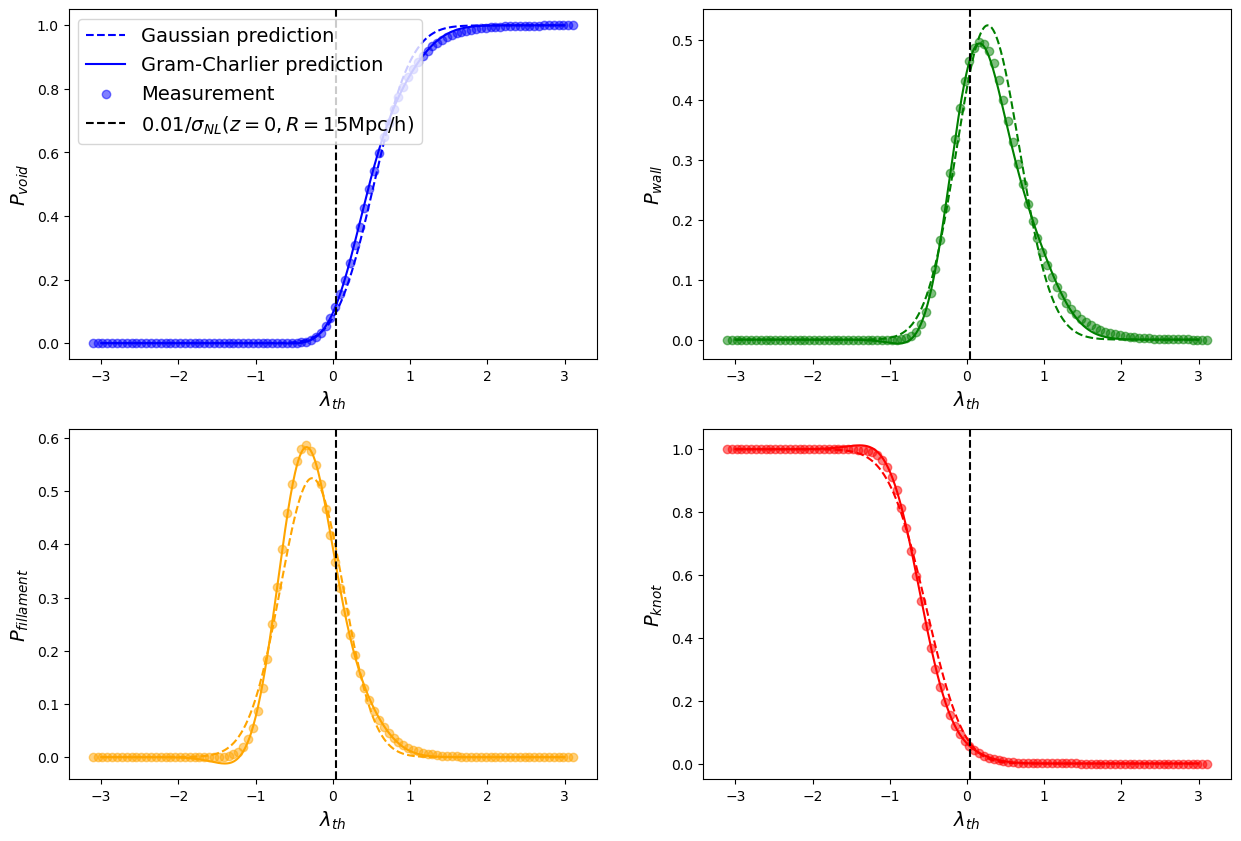
Figure 3: Probability of the environment as a function of the threshold for a Gaussian random field (dashed lines), Gram-Charlier (solid lines), and measurement in the simulations (dots) at R=15 Mpc/h and z=0. The vertical black line is the threshold $\Lambda_{\rm th}=0.01$ (thus $\lambda_{\text{th}}=\Lambda_{\rm th}/\sigma_{\text{NL}}$) used in the paper.

4 Mild non-Gaussian corrections to cosmic web abundances

Relying on Gaussian random fields is valid only in the linear regime of structure formation. However, at low redshift/small scales, more and more non-Gaussianities appear in the density field and corrections to the Gaussian predictions need to be accounted for. To improve our previous Gaussian predictions, we now propose to work with a probability distribution function ${\cal P}(X)$ which is no more Gaussian but includes non-linearities in a perturbative manner. In practice, we will use a Gram-Charlier expansion following previous works in the literature including Pogosyan et al. (2009); Gay et al. (2012); Codis et al. (2013).

4.1 Gram-Charlier expansion of the joint distribution

For a set $X$ of random fields, the Gram-Charlier expansion of the joint PDF reads

$${\cal P}(X)={\cal P_{G}}(X)\left[1+\sum_{n=3}^{\infty}\frac{1}{n!}Tr[\langle X^{n}\rangle_{GC}.h_{n}(X)]\right],$$ (26)

where ${\cal P_{G}}(X)$ is a Gaussian kernel as defined in equation (12), $h_{n}(x)$ are the Hermite tensors $h_{n}(X)=(-1)^{n}{\cal P_{G}}^{-1}(X)\partial^{n}{\cal P_{G}}(X)/\partial X^{n}$ and $\langle X^{n}\rangle_{GC}=\langle h_{n}(X)\rangle$ are the Gram Charlier coefficients.

For our rotation-invariant variables $J_{1},J_{2},J_{3}$, this translates into the following expression

$$\begin{split}{\cal P}(J_{1},J_{2},J_{3})&={\cal P_{G}}(J_{1},J_{2},J_{3})\Biggl{[}1+\sum_{n=3}^{\infty}\sum_{k,l}^{k+2l=n}\frac{(-1)^{l}5^{l}\times 3}{k!(3+2l)!!}\langle J_{1}^{k}J_{2}^{l}\rangle_{GC}H_{k}(J_{1})L_{l}^{(3/2)}\left(\frac{5}{2}J_{2}\right)\\ &+\sum_{n=3}^{\infty}\sum_{k}^{k+3=n}\frac{25}{k!\times 21}\langle J_{1}^{k}J_{3}\rangle_{GC}H_{k}(J_{1})J_{3}+\sum_{n=5}^{\infty}\sum_{k,l,m=1}^{k+2l+3m=n}\frac{c_{lm}}{k!}\langle J_{1}^{k}J_{2}^{l}J_{3}^{m}\rangle_{GC}H_{k}(J_{1})F_{lm}(J_{2},J_{3})\Biggr{]},\end{split}$$ (27)

where ${\cal P_{G}}(J_{1},J_{2},J_{3})$ is the Gaussian case given by equation (17), $H_{n}$ are the successive Hermite polynomials, $L_{l}^{(\alpha)}(x)$ are the generalized Laguerre polynomials, $c_{lm}$ are the normalization coefficients that we let undetermined and the orthogonal polynomials $F_{lm}$ associated with $J_{2}$ and $J_{3}$ are such that

$$\int_{0}^{\infty}{\rm d}J_{2}\int_{-J_{2}^{3/2}}^{J_{2}^{3/2}}{\rm d}J_{3}{\cal P_{G}}(J_{1},J_{2},J_{3})F_{lm}(J_{2},J_{3})F_{l^{\prime}m^{\prime}}(J_{2},J_{3})=\delta_{l}^{l^{\prime}}\delta_{m}^{m^{\prime}}.$$

We have, for example, these special cases: $F_{l0}=\sqrt{3\times 2^{l}\times l!/(3+2l)!!}\times L_{l}^{3/2}({5}J_{2}/2)$ and $F_{01}={5}J_{3}/{\sqrt{21}}$.

Here, we will focus on the first corrective term, $n=3$, such that

$$\begin{split}{\cal P}(J_{1},J_{2},J_{3})&={\cal P_{G}}(J_{1},J_{2},J_{3})\Biggl{[}1+\frac{1}{6}\langle J_{1}^{3}\rangle_{GC}H_{3}(J_{1})-\langle J_{1}J_{2}\rangle_{GC}H_{1}(J_{1})L_{1}^{(3/2)}\left(\frac{5}{2}J_{2}\right)+\frac{25}{21}\langle J_{3}\rangle_{GC}J_{3}\Biggr{]}+o(\sigma_{0}^{2}).\end{split}$$ (28)

The Gram-Charlier cumulants read

$$\langle J_{1}^{3}\rangle_{GC}=\langle H_{3}(J_{1})\rangle,\qquad\langle J_{1}J_{2}\rangle_{GC}=-\frac{2}{5}\left\langle H_{1}(J_{1})L_{1}^{(3/2)}\left(\frac{5}{2}J_{2}\right)\right\rangle,\qquad\langle J_{3}\rangle_{GC}=\langle J_{3}\rangle,$$ (29)

such that we finally obtain the Gram-Charlier expression at first non-linear order (NLO)

$${\cal P}(J_{1},J_{2},J_{3})={\cal P_{G}}(J_{1},J_{2},J_{3})\Biggl{[}1+\frac{1}{6}\langle J_{1}^{3}\rangle(J_{1}^{3}-3J_{1})+\frac{5}{2}\langle J_{1}J_{2}\rangle J_{1}(J_{2}-1)+\frac{25}{21}\langle J_{3}\rangle J_{3}\Biggr{]}+o(\sigma_{0}^{2}).$$ (30)

Three cumulants appear in the next-to-leading-order Gram-Charlier probability distribution function (equation (30)): $\langle J_{1}^{3}\rangle$, $\langle J_{1}J_{2}\rangle$ and $\langle J_{3}\rangle$. In Eulerian perturbation theory, those cumulants are linear in $\sigma_{0}$ at tree order and we thus introduce the reduced cumulants $S_{3}=\langle J_{1}^{3}\rangle/\sigma_{0}$, $U_{3}=\langle J_{1}J_{2}\rangle/\sigma_{0}$ and $V_{3}=\langle J_{3}\rangle/\sigma_{0}$ which are constant in time at tree order. For example, $S_{3}$ is the usual cosmological skewness whose analytical prediction at tree order is well-known (for example, Peebles 1980; Juszkiewicz et al. 1993; Lokas et al. 1995; Colombi et al. 2000). The other two reduced cumulants can be computed in a similar manner that we describe in Appendix A. In figure 4, we display the resulting tree-order cumulants as a function of the smoothing scale in dashed black, compared to the measurements in the simulation at different redshifts (as shown with different colors). We see a good agreement at almost all smoothing scales and redshifts as the prediction is almost always within the error bars. For large smoothing scales, the error bars increase due to the finite volume of the Quijote simulation which thus misses large wave modes. As expected, at low redshift and small smoothing scales, departures from tree-order predictions are seen as the non-linearities increase. In this work, we focus on mildly non-linear scales (about 10 Mpc/h and above) where a perturbative treatment is accurate, as illustrated by the values of the cumulants depicted in this figure.

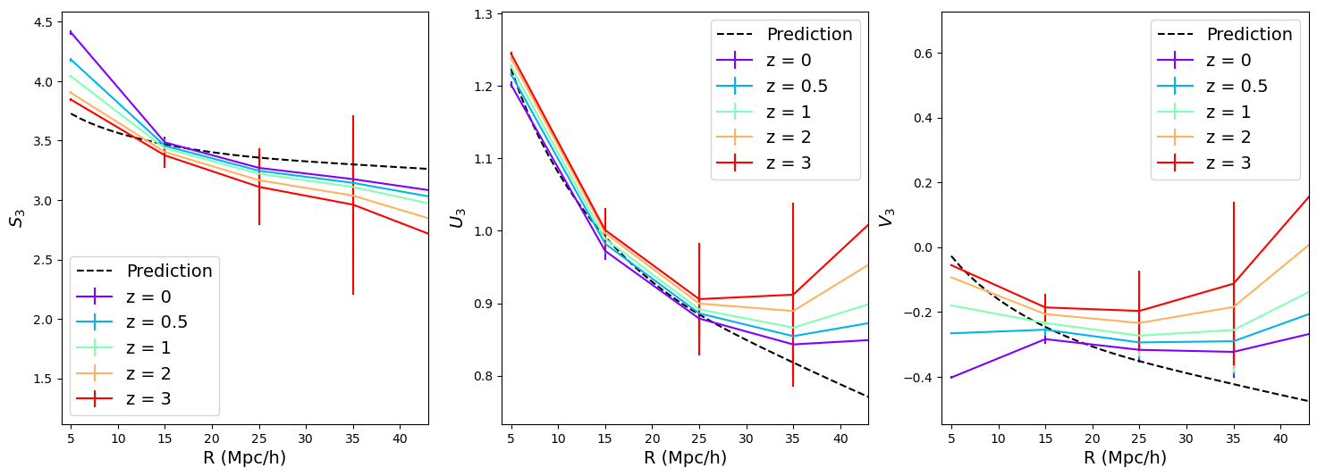
Figure 4: Cumulants $S_{3}$, $U_{3}$ and $V_{3}$ as a function of the smoothing scale R. The dashed black line is the analytical prediction. The color lines are the measurements from the simulations at different redshifts.

4.2 Cosmic web abundances at next-to-leading order

We now turn to the explicit computation of the probability of different cosmic environments at next-to-leading order in the Gram-Charlier formalism. Let us first rewrite the Gram-Charlier expansion of the joint distribution of the rotational invariants of the tidal tensor as

$${\cal P}(J_{1},J_{2},J_{3})={\cal P_{G}}(J_{1},J_{2},J_{3})+\sigma_{0}{\cal P}^{(3)}(J_{1},J_{2},J_{3})+O(\sigma_{0}^{2}),$$ (31)

where $\cal{P_{G}}$ is the Gaussian part and ${\cal P}^{(3)}$ the first non-Gaussian corrective term

$${\cal P}^{(3)}(J_{1},J_{2},J_{3})=\frac{25\sqrt{5}}{12\pi}\exp\left[-\frac{J_{1}^{2}}{2}-\frac{5J_{2}}{2}\right]\left(\frac{1}{6}\left(J_{1}^{3}-3J_{1}\right)S_{3}+\frac{5}{2}J_{1}(J_{2}-1)U_{3}+\frac{25}{21}J_{3}V_{3}\right).$$ (32)

Integrating this distribution function over the constraints given in equations (18) to (21) will give us the expression of the probability of a given environment $(E)$ as

$$\begin{split}P_{(E)}(\lambda_{\rm th})&=P_{G,(E)}(\lambda_{\rm th})+\sigma_{0}P^{(3)}_{(E)}(\lambda_{\rm th})\\ &=P_{G,(E)}(\lambda_{\rm th})+\sigma_{0}\bigl{[}s_{(E)}(\lambda_{\rm th})S_{3}+u_{(E)}(\lambda_{th,})U_{3}+v_{(E)}(\lambda_{\rm th})V_{3}\bigr{]},\end{split}$$ (33)

where $s,u,v$ are threshold-dependent functions and where the Gaussian probability of the environments was derived in equations (22) to (25).

Again two degrees of freedom can be integrated out and one remains to be done numerically. The resulting expressions for $s(\lambda_{\rm th})$, $u(\lambda_{\rm th})$ and $v(\lambda_{\rm th})$ in each environment are given below (written in terms of 1D integrals over $J_{2}$).

4.2.1 Void

For voids, we get

$$\begin{split}s_{\text{void}}(\lambda_{\rm th})&=\int_{0}^{\infty}\frac{25\sqrt{5}}{144\pi}e^{\frac{1}{2}(-9)\left(J_{2}+\lambda_{\rm th}^{2}\right)}\Biggl{[}-3\sqrt{2\pi}e^{2J_{2}+\frac{9\lambda_{\rm th}^{2}}{2}}\text{erf}\left(\frac{2\sqrt{J_{2}}-3\lambda_{\rm th}}{\sqrt{2}}\right)+3\sqrt{2\pi}e^{2J_{2}+\frac{9\lambda_{\rm th}^{2}}{2}}\text{erf}\left(\frac{\sqrt{\text{J2}}-3\lambda_{\rm th}}{\sqrt{2}}\right)\\ &+\sqrt{J_{2}}e^{3\sqrt{J_{2}}\lambda_{\rm th}}\bigl{[}e^{3\sqrt{J_{2}}\lambda_{\rm th}}(-48J_{2}^{3/2}\lambda_{\rm th}+16J_{2}^{2}+36J_{2}\lambda_{\rm th}^{2}-27\sqrt{J_{2}}\lambda_{\rm th}+14J_{2}+12)-6e^{\frac{3J_{2}}{2}}\bigr{]}\Biggr{]}\\ &+\frac{25\sqrt{5}}{36\pi}J_{2}^{3/2}e^{6\sqrt{J_{2}}\lambda_{\rm th}-\frac{9J_{2}}{2}-\frac{9\lambda_{\rm th}^{2}}{2}}\left(1-\left(2\sqrt{J_{2}}-3\lambda_{\rm th}\right)^{2}\right){\rm d}J_{2},\end{split}$$ (34)

 

$$\begin{split}u_{\text{void}}(\lambda_{\rm th})&=\int_{0}^{\infty}-\frac{125\sqrt{5}}{96\pi}(J_{2}-1)e^{\frac{1}{2}(-9)\left(J_{2}+\lambda_{\rm th}^{2}\right)}\Biggl{[}-3\sqrt{2\pi}e^{2J_{2}+\frac{9\lambda_{\rm th}^{2}}{2}}\left(J_{2}-9\lambda_{\rm th}^{2}-1\right)\text{erf}\left(\frac{2\sqrt{J_{2}}-3\lambda_{\rm th}}{\sqrt{2}}\right)\\ &+3\sqrt{2\pi}e^{2J_{2}+\frac{9\lambda_{\rm th}^{2}}{2}}\left(J_{2}-9\lambda_{\rm th}^{2}-1\right)\text{erf}\left(\frac{\sqrt{J_{2}}-3\lambda_{\rm th}}{\sqrt{2}}\right)-2e^{6\sqrt{J_{2}}\lambda_{\rm th}}\left(4J_{2}^{3/2}+6\sqrt{J_{2}}+9\lambda_{\rm th}\right)+6e^{3\sqrt{J_{2}}\lambda_{\rm th}+\frac{3J_{2}}{2}}\left(\sqrt{J_{2}}+3\lambda_{\rm th}\right)\Biggr{]}\\ &-\frac{125\sqrt{5}}{12\pi}(J_{2}-1)J_{2}^{3/2}e^{6\sqrt{J_{2}}\lambda_{\rm th}-\frac{9J_{2}}{2}-\frac{9\lambda_{\rm th}^{2}}{2}}{\rm d}J_{2},\end{split}$$ (35)

 

$$\begin{split}v_{\text{void}}(\lambda_{\rm th})&=\int_{0}^{\infty}\frac{625\sqrt{5}}{4032\pi}e^{-\frac{5J_{2}}{2}}\Biggl{[}-\sqrt{2\pi}\biggl{[}-4J_{2}^{3}+9J_{2}^{2}+243(5-2J_{2})\lambda_{\rm th}^{4}+81((J_{2}-4)J_{2}+5)\lambda_{\rm th}^{2}-18J_{2}+729\lambda_{\rm th}^{6}+15\biggr{]}\\ &\times\text{erf}\left(\frac{3\lambda_{\rm th}-2\sqrt{J_{2}}}{\sqrt{2}}\right)+\sqrt{2\pi}\biggl{[}-4J_{2}^{3}+9J_{2}^{2}+243(5-2J_{2})\lambda_{\rm th}^{4}+81((J_{2}-4)J_{2}+5)\lambda_{\rm th}^{2}-18J_{2}+729\lambda_{\rm th}^{6}+15\biggr{]}\text{erf}\left(\frac{3\lambda_{\rm th}-\sqrt{J_{2}}}{\sqrt{2}}\right)\\ &+2e^{-\frac{1}{2}\left(\sqrt{J_{2}}-3\lambda_{\rm th}\right)^{2}}\biggl{[}J_{2}^{3/2}\left(-\left(45\lambda_{\rm th}^{2}+13\right)\right)+12J_{2}^{2}\lambda_{\rm th}+4J_{2}^{5/2}-9J_{2}\lambda_{\rm th}\left(15\lambda_{\rm th}^{2}+7\right)+3\sqrt{J_{2}}\left(27\lambda_{\rm th}^{4}+36\lambda_{\rm th}^{2}+5\right)\\ &+9\lambda_{\rm th}\left(27\lambda_{\rm th}^{4}+42\lambda_{\rm th}^{2}+11\right)\biggr{]}-2e^{-\frac{1}{2}\left(2\sqrt{J_{2}}-3\lambda_{\rm th}\right)^{2}}\biggl{[}J_{2}^{3/2}\left(4-36\lambda_{\rm th}^{2}\right)+3J_{2}^{2}\lambda_{\rm th}+2J_{2}^{5/2}+J_{2}\left(18\lambda_{\rm th}-54\lambda_{\rm th}^{3}\right)\\ &+6\sqrt{J_{2}}\left(27\lambda_{\rm th}^{4}+36\lambda_{\rm th}^{2}+5\right)+9\lambda_{\rm th}\left(27\lambda_{\rm th}^{4}+42\lambda_{\rm th}^{2}+11\right)\biggr{]}\Biggr{]}{\rm d}J_{2},\end{split}$$ (36)

where $\text{erf}(z)$ is again the error function. Once that analytical expression is obtained, we can perform the numerical integration over $J_{2}$. We display $s(\lambda_{\rm th})$, $u(\lambda_{\rm th})$ and $v(\lambda_{\rm th})$ as a function of the threshold in 5.

4.2.2 Wall

For walls, the same procedure gives

$$\begin{split}s_{\text{wall}}(\lambda_{\rm th})&=\int_{0}^{\infty}\frac{25\sqrt{5}}{48\pi}e^{-\frac{9J_{2}}{2}}\Biggl{[}-\sqrt{2\pi}e^{2J_{2}}\text{erf}\left(\frac{3\lambda_{\rm th}-2\sqrt{J_{2}}}{\sqrt{2}}\right)+\sqrt{2\pi}e^{2J_{2}}\text{erf}\left(\frac{\sqrt{J_{2}}+3\lambda_{\rm th}}{\sqrt{2}}\right)+\sqrt{J_{2}}\left(-e^{\frac{1}{2}(-3)\lambda_{\rm th}\left(2\sqrt{J_{2}}+3\lambda_{\rm th}\right)}\right)\\ &\times\left(e^{9\sqrt{J_{2}}\lambda_{\rm th}}\left(-9\sqrt{J_{2}}\lambda_{\rm th}+6J_{2}+4\right)+2e^{\frac{3J_{2}}{2}}\right)\Biggr{]}{\rm d}J_{2},\end{split}$$ (37)

 

$$\begin{split}u_{\text{wall}}(\lambda_{\rm th})&=\int_{0}^{\infty}\frac{125\sqrt{5}}{32\pi}e^{-\frac{9J_{2}}{2}}(J_{2}-1)\Biggl{[}-\sqrt{2\pi}e^{2J_{2}}\left(J_{2}-9\lambda_{\rm th}^{2}-1\right)\text{erf}\left(\frac{\sqrt{J_{2}}+3\lambda_{\rm th}}{\sqrt{2}}\right)\\ &+\sqrt{2\pi}e^{2J_{2}}\left(J_{2}-9\lambda_{\rm th}^{2}-1\right)\text{erf}\left(\frac{3\lambda_{\rm th}-2\sqrt{J_{2}}}{\sqrt{2}}\right)-2e^{\frac{1}{2}(-3)\lambda_{\rm th}\left(2\sqrt{J_{2}}+3\lambda_{\rm th}\right)}\biggl{[}e^{9\sqrt{J_{2}}\lambda_{\rm th}}\left(2\sqrt{J_{2}}+3\lambda_{\rm th}\right)+e^{\frac{3J_{2}}{2}}\left(\sqrt{J_{2}}-3\lambda_{\rm th}\right)\biggr{]}\Biggr{]}{\rm d}J_{2},\end{split}$$ (38)

 

$$\begin{split}&v_{\text{wall}}(\lambda_{\rm th})=\int_{0}^{\infty}-\frac{625\sqrt{5}}{4032\pi}e^{-\frac{5J_{2}}{2}}\Biggl{[}-\sqrt{2\pi}\biggl{[}-4J_{2}^{3}+9J_{2}^{2}+243(5-2J_{2})\lambda_{\rm th}^{4}+81((J_{2}-4)J_{2}+5)\lambda_{\rm th}^{2}-18J_{2}+729\lambda_{\rm th}^{6}+15\biggl{]}\text{erf}\left(\frac{3\lambda_{\rm th}-2\sqrt{J_{2}}}{\sqrt{2}}\right)\\ &+\sqrt{2\pi}\biggl{[}-4J_{2}^{3}+9J_{2}^{2}+243(5-2J_{2})\lambda_{\rm th}^{4}+81((J_{2}-4)J_{2}+5)\lambda_{\rm th}^{2}-18J_{2}+729\lambda_{\rm th}^{6}+15\biggr{]}\text{erf}\left(\frac{\sqrt{J_{2}}+3\lambda_{\rm th}}{\sqrt{2}}\right)\\ &-2e^{-\frac{1}{2}\left(2\sqrt{J_{2}}-3\lambda_{\rm th}\right)^{2}}\biggl{[}J_{2}^{3/2}\left(4-36\lambda_{\rm th}^{2}\right)+3J_{2}^{2}\lambda_{\rm th}+2J_{2}^{5/2}+J_{2}\left(18\lambda_{\rm th}-54\lambda_{\rm th}^{3}\right)+6\sqrt{J_{2}}\left(27\lambda_{\rm th}^{4}+36\lambda_{\rm th}^{2}+5\right)+9\lambda_{\rm th}\left(27\lambda_{\rm th}^{4}+42\lambda_{\rm th}^{2}+11\right)\biggr{]}\\ &+2e^{-\frac{1}{2}\left(\sqrt{J_{2}}+3\lambda_{\rm th}\right)^{2}}\biggl{[}J_{2}^{3/2}\left(45\lambda_{\rm th}^{2}+13\right)+12J_{2}^{2}\lambda_{\rm th}-4J_{2}^{5/2}-9J_{2}\lambda_{\rm th}\left(15\lambda_{\rm th}^{2}+7\right)-3\sqrt{J_{2}}\left(27\lambda_{\rm th}^{4}+36\lambda_{\rm th}^{2}+5\right)+9\lambda_{\rm th}\left(27\lambda_{\rm th}^{4}+42\lambda_{\rm th}^{2}+11\right)\biggr{]}\Biggr{]}{\rm d}J_{2}.\end{split}$$ (39)

4.2.3 Filament

For filaments we get

$$\begin{split}s_{\text{filament}}(\lambda_{\rm th})&=\int_{0}^{\infty}-\frac{25\sqrt{5}}{144\pi}e^{\frac{1}{2}(-3)\left(4\sqrt{J_{2}}\lambda_{\rm th}+3J_{2}+3\lambda_{\rm th}^{2}\right)}\Biggl{[}3\sqrt{2\pi}e^{\frac{1}{2}\left(2\sqrt{J_{2}}+3\lambda_{\rm th}\right)^{2}}\text{erf}\left(\frac{2\sqrt{J_{2}}+3\lambda_{\rm th}}{\sqrt{2}}\right)\\ &+3\sqrt{2\pi}e^{\frac{1}{2}\left(2\sqrt{J_{2}}+3\lambda_{\rm th}\right)^{2}}\text{erf}\left(\frac{\sqrt{J_{2}}-3\lambda_{\rm th}}{\sqrt{2}}\right)-3\sqrt{J_{2}}\left(2e^{9\sqrt{J_{2}}\lambda_{\rm th}+\frac{3J_{2}}{2}}+9\sqrt{J_{2}}\lambda_{\rm th}+6J_{2}+4\right)\Biggr{]}{\rm d}J_{2},\end{split}$$ (40)

 

$$\begin{split}u_{\text{filament}}(\lambda_{\rm th})&=\int_{0}^{\infty}-\frac{125\sqrt{5}}{48\pi}(J_{2}-1)\Biggl{[}3\sqrt{\frac{\pi}{2}}e^{-\frac{5J_{2}}{2}}\left(J_{2}-9\lambda_{\rm th}^{2}-1\right)\text{erf}\left(\frac{3\lambda_{\rm th}-\sqrt{J_{2}}}{\sqrt{2}}\right)-\frac{3}{2}e^{\frac{1}{2}(-3)\left(4\sqrt{J_{2}}\lambda_{\rm th}+3J_{2}+3\lambda_{\rm th}^{2}\right)}\\ &\times[\sqrt{2\pi}e^{\frac{1}{2}\left(2\sqrt{J_{2}}+3\lambda_{\rm th}\right)^{2}}\left(J_{2}-9\lambda_{\rm th}^{2}-1\right)\text{erf}\left(\frac{2\sqrt{J_{2}}+3\lambda_{\rm th}}{\sqrt{2}}\right)+6\lambda_{\rm th}\left(e^{9\sqrt{J_{2}}\lambda_{\rm th}+\frac{3J_{2}}{2}}-1\right)+2\sqrt{J_{2}}\left(e^{9\sqrt{J_{2}}\lambda_{\rm th}+\frac{3J_{2}}{2}}+2\right)]\Biggr{]}{\rm d}J_{2},\end{split}$$ (41)

 

$$\begin{split}v_{\text{filament}}(\lambda_{\rm th})&=\int_{0}^{\infty}\frac{625\sqrt{5}}{4032\pi}e^{-\frac{5J_{2}}{2}}\Biggl{[}-\sqrt{2\pi}[-4J_{2}^{3}+9J_{2}^{2}+243(5-2J_{2})\lambda_{\rm th}^{4}+81((J_{2}-4)J_{2}+5)\lambda_{\rm th}^{2}-18J_{2}+729\lambda_{\rm th}^{6}+15]\text{erf}\left(\frac{3\lambda_{\rm th}-\sqrt{J_{2}}}{\sqrt{2}}\right)\\ &+\sqrt{2\pi}[-4J_{2}^{3}+9J_{2}^{2}+243(5-2J_{2})\lambda_{\rm th}^{4}+81((J_{2}-4)J_{2}+5)\lambda_{\rm th}^{2}-18J_{2}+729\lambda_{\rm th}^{6}+15]\text{erf}\left(\frac{2\sqrt{J_{2}}+3\lambda_{\rm th}}{\sqrt{2}}\right)-2e^{-\frac{1}{2}\left(\sqrt{J_{2}}-3\lambda_{\rm th}\right)^{2}}\\ &\times[J_{2}^{3/2}\left(-\left(45\lambda_{\rm th}^{2}+13\right)\right)+12J_{2}^{2}\lambda_{\rm th}+4J_{2}^{5/2}-9J_{2}\lambda_{\rm th}\left(15\lambda_{\rm th}^{2}+7\right)+3\sqrt{J_{2}}\left(27\lambda_{\rm th}^{4}+36\lambda_{\rm th}^{2}+5\right)+9\lambda_{\rm th}\left(27\lambda_{\rm th}^{4}+42\lambda_{\rm th}^{2}+11\right)]\\ &+e^{-\frac{1}{2}\left(2\sqrt{J_{2}}+3\lambda_{\rm th}\right)^{2}}[8J_{2}^{3/2}\left(9\lambda_{\rm th}^{2}-1\right)+6J_{2}^{2}\lambda_{\rm th}-4J_{2}^{5/2}-36J_{2}\lambda_{\rm th}\left(3\lambda_{\rm th}^{2}-1\right)\\ &-12\sqrt{J_{2}}\left(27\lambda_{\rm th}^{4}+36\lambda_{\rm th}^{2}+5\right)+18\lambda_{\rm th}\left(27\lambda_{\rm th}^{4}+42\lambda_{\rm th}^{2}+11\right)]\Biggr{]}{\rm d}J_{2}.\end{split}$$ (42)

4.2.4 Knots

Finally, for knots:

$$\begin{split}s_{\text{knot}}(\lambda_{\rm th})&=\int_{0}^{\infty}\frac{25\sqrt{5}}{144\pi}e^{\frac{1}{2}(-3)\left(4\sqrt{J_{2}}\lambda_{\rm th}+3J_{2}+3\lambda_{\rm th}^{2}\right)}\Biggl{[}-3\sqrt{2\pi}e^{\frac{1}{2}\left(2\sqrt{J_{2}}+3\lambda_{\rm th}\right)^{2}}\text{erf}\left(\frac{\sqrt{J_{2}}+3\lambda_{\rm th}}{\sqrt{2}}\right)+3\sqrt{2\pi}e^{\frac{1}{2}\left(2\sqrt{J_{2}}+3\lambda_{\rm th}\right)^{2}}\text{erf}\left(\frac{2\sqrt{J_{2}}+3\lambda_{\rm th}}{\sqrt{2}}\right)\\ &-\sqrt{J_{2}}\biggl{[}48J_{2}^{3/2}\lambda_{\rm th}+16J_{2}^{2}+36J_{2}\lambda_{\rm th}^{2}-6e^{3\sqrt{J_{2}}\lambda_{\rm th}+\frac{3J_{2}}{2}}+27\sqrt{J_{2}}\lambda_{\rm th}+14J_{2}+12\biggr{]}\Biggr{]}\\ &+\frac{25\sqrt{5}}{36\pi}J_{2}^{3/2}e^{\frac{1}{2}(-3)\left(4\sqrt{J_{2}}\lambda_{\rm th}+3J_{2}+3\lambda_{\rm th}^{2}\right)}\left(12\sqrt{J_{2}}\lambda_{\rm th}+4J_{2}+9\lambda_{\rm th}^{2}-1\right){\rm d}J_{2},\end{split}$$ (43)

 

$$\begin{split}u_{\text{knot}}(\lambda_{\rm th})&=\int_{0}^{\infty}\frac{125\sqrt{5}}{96\pi}(J_{2}-1)e^{\frac{1}{2}(-3)\left(4\sqrt{J_{2}}\lambda_{\rm th}+3J_{2}+3\lambda_{\rm th}^{2}\right)}\Biggl{[}-3\sqrt{2\pi}e^{\frac{1}{2}\left(2\sqrt{J_{2}}+3\lambda_{\rm th}\right)^{2}}\left(J_{2}-9\lambda_{\rm th}^{2}-1\right)\text{erf}\left(\frac{2\sqrt{J_{2}}+3\lambda_{\rm th}}{\sqrt{2}}\right)\\ &+3\sqrt{2\pi}e^{\frac{1}{2}\left(2\sqrt{J_{2}}+3\lambda_{\rm th}\right)^{2}}\left(J_{2}-9\lambda_{\rm th}^{2}-1\right)\text{erf}\left(\frac{\sqrt{J_{2}}+3\lambda_{\rm th}}{\sqrt{2}}\right)-8J_{2}^{3/2}-18\lambda_{\rm th}\left(e^{3\sqrt{J_{2}}\lambda_{\rm th}+\frac{3J_{2}}{2}}-1\right)+6\sqrt{J_{2}}\left(e^{3\sqrt{J_{2}}\lambda_{\rm th}+\frac{3J_{2}}{2}}-2\right)\Biggr{]}\\ &+\frac{125\sqrt{5}}{12\pi}(J_{2}-1)J_{2}^{3/2}e^{\frac{1}{2}(-3)\left(4\sqrt{J_{2}}\lambda_{\rm th}+3J_{2}+3\lambda_{\rm th}^{2}\right)}{\rm d}J_{2},\end{split}$$ (44)

 

$$\begin{split}&v_{\text{knot}}(\lambda_{\rm th})=\int_{0}^{\infty}-\frac{625\sqrt{5}}{4032\pi}e^{-\frac{5J_{2}}{2}}\Biggl{[}-\sqrt{2\pi}\biggl{[}-4J_{2}^{3}+9J_{2}^{2}+243(5-2J_{2})\lambda_{\rm th}^{4}+81((J_{2}-4)J_{2}+5)\lambda_{\rm th}^{2}-18J_{2}+729\lambda_{\rm th}^{6}+15\biggr{]}\text{erf}\left(\frac{\sqrt{J_{2}}+3\lambda_{\rm th}}{\sqrt{2}}\right)\\ &+\sqrt{2\pi}\biggl{[}-4J_{2}^{3}+9J_{2}^{2}+243(5-2J_{2})\lambda_{\rm th}^{4}+81((J_{2}-4)J_{2}+5)\lambda_{\rm th}^{2}-18J_{2}+729\lambda_{\rm th}^{6}+15\biggr{]}\text{erf}\left(\frac{2\sqrt{J_{2}}+3\lambda_{\rm th}}{\sqrt{2}}\right)\\ &+e^{-\frac{1}{2}\left(2\sqrt{J_{2}}+3\lambda_{\rm th}\right)^{2}}\biggl{[}8J_{2}^{3/2}\left(9\lambda_{\rm th}^{2}-1\right)+6J_{2}^{2}\lambda_{\rm th}-4J_{2}^{5/2}-36J_{2}\lambda_{\rm th}\left(3\lambda_{\rm th}^{2}-1\right)-12\sqrt{J_{2}}\left(27\lambda_{\rm th}^{4}+36\lambda_{\rm th}^{2}+5\right)+18\lambda_{\rm th}\left(27\lambda_{\rm th}^{4}+42\lambda_{\rm th}^{2}+11\right)\biggr{]}\\ &+2e^{-\frac{1}{2}\left(\sqrt{J_{2}}+3\lambda_{\rm th}\right)^{2}}\biggl{[}J_{2}^{3/2}\left(-\left(45\lambda_{\rm th}^{2}+13\right)\right)-12J_{2}^{2}\lambda_{\rm th}+4J_{2}^{5/2}+9J_{2}\lambda_{\rm th}\left(15\lambda_{\rm th}^{2}+7\right)+3\sqrt{J_{2}}\left(27\lambda_{\rm th}^{4}+36\lambda_{\rm th}^{2}+5\right)\\ &-9\lambda_{\rm th}\left(27\lambda_{\rm th}^{4}+42\lambda_{\rm th}^{2}+11\right)\biggr{]}\Biggr{]}{\rm d}J_{2}.\end{split}$$ (45)

Plugging the previous expressions for the $s,u,v$ functions in equation (33) finally allows us to compute the next-to-leading order correction to the (threshold-dependent) probability of the different cosmic environments in the T-web classification.

As for the Gaussian case, we choose to measure a rarity threshold in the simulations hence to plug in the non-linear variance measured in the simulation as the normalization factor appearing in the threshold $\lambda_{\rm th}$. An alternative option to try and keep a meaningful threshold selection in terms of abundance/rarity could be to work with a filling factor, as mentioned at the end of Section 3.

The probability of the different environments as a function of redshift is displayed in figure 2 which was already partially described in section 3 for the Gaussian case. We now focus on the solid lines which represent the Gram-Charlier correction described in this section. For every environment, redshift, and smoothing scale, the results obtained with the Gram-Charlier always improve the prediction over the Gaussian case. The agreement between the simulation and our non-linear model is exquisite. Only at the most non-linear scales (very low redshift and small smoothing scale), the predictions start to become slightly different from the measurements although the NLO correction always improves upon the Gaussian case. We can also look at the probability of voids, walls, filaments, and knots as a function of the threshold in figure 3 which was also already partially described in section 3. We see that the Gram-Charlier correction not only improves the prediction over the Gaussian case but provides us with an extremely accurate prediction at all the relevant thresholds and for almost the whole spectrum of field values. Let us look at the contribution of each function that appears in our Gram-Charlier expansion: $s_{(E)}(\lambda_{\rm th})$, $u_{(E)}(\lambda_{\rm th})$ and $v_{(E)}(\lambda_{\rm th})$ in equation (33) as shown in figure 5. One can note that $S_{3}$ is always larger than $U_{3}$ and $V_{3}$, implying that $s(\lambda_{\text{th}})$ is typically the dominant correction to the Gaussian case (and is actually related to the non-linear evolution of the threshold). This is the reason why our Gaussian model for the evolution of the cosmic web abundances already gives a fairly accurate prescription. The higher-order non-linear corrections are then modulated by the functions $s,u,v$ depending on the chosen threshold.

5 Discussion and conclusion

Using the T-web classification with a rarity threshold $\lambda_{\text{th}}={(\Lambda_{\rm th}=0.01)}/{\sigma_{\text{NL}}}$ (a commonly $\Lambda_{\rm th}$ value used in the literature), we have described a theoretical framework to accurately model the probability of voids, walls, filaments, and knots in the cosmic web. More precisely, since this computation requires the knowledge of the joint probability distribution of the eigenvalues of the Hessian of the gravitational potential, we model an analogous object which is the joint distribution between maximally de-correlated, rotational invariants that are polynomial in the Cartesian matrix components.

We first focused on the linear regime of structure formation where the density field is Gaussian (assuming Gaussian initial conditions) and where the distribution of the eigenvalues of the Hessian of the gravitational potential – then a Gaussian field – are known. We found in that case that normalizing the rarity threshold $\lambda_{\rm th}$ by the non-linear variance was surprisingly accurate with respect to measurements of the environments probabilities in the Quijote simulation in regimes where $\sigma\lesssim 0.1$ and capturing most of the redshift and scale dependence (see figure 2).

To probe the mildly non-linear regime, we then accounted for corrections to the Gaussian case in a perturbative manner relying on a Gram-Charlier expansion at first non-linear order (equation (30)) for the joint distribution of our rotational invariants, and tree-order Eulerian perturbation theory to compute the Gram-Charlier coefficients. We showed that this correction to the Gaussian case increases the accuracy of predictions for the probability of cosmic environments at all considered redshifts and smoothing scales with threshold $\lambda_{\text{th}}={0.01}/{\sigma_{\text{NL}}}$ (see figure 2), but also when varying the threshold at fixed redshift and smoothing scale (see figure 3 for a reference case at $z=0$ and $R=15$ Mpc/h).

As a conclusion, all redshift and scale-dependent evolution of T-web cosmic abundances that have been previously observed in numerical simulations are shown to be predictable from first principle. In addition, having a precise theoretical model not only allows to benchmark simulations but also understand how these features depend on choices like the threshold or on the background cosmological model. This information can be readily extracted from the predictions we provide here (without the need for running simulations, post-processing them, etc.). This is notably important when one wants to use these cosmic web elements as a cosmological probe (to go typically beyond the power spectrum), hence requiring a cost-effective inference pipeline. We leave investigations along this line for future works. Let us also emphasize that we have assumed Gaussian initial conditions in this work, but primordial non-Gaussianities could easily be added to the formalism (following for instance Codis et al. (2013)) in which case a careful study of how much cosmic web abundance depends on the physics of the primordial Universe could be performed.

Looking at figure 3 for the direct result of the threshold-dependent modulation of the non-Gaussian cumulants appearing in the Gram-Charlier expansion of figure 5, we observe that the different probabilities can fluctuate a lot when changing the threshold, as was pointed out for instance in Forero-Romero et al. (2009) which studied the impact of the choice of the threshold on the percolation and fragmentation of the cosmic web. With the present formalism, all this information can be described from first-principles, which can be very useful in defining a physically motivated threshold rather than visual inspection. Working with the abundance or rarity of an environment or with a filling factor could definitely help in that direction.

Another possible extension of this work could be to perform a multi-scale analysis in order to study the properties of halos depending on their environment. The T-web description developed here would provide the constrained environment (as often used in simulations) while the fields on a smaller scale would characterize the halo. However, let us note that the T-web classification is a rather rough description of the cosmic web and more sophisticated frameworks have already been developed in the literature. Interestingly though, most analyses studying environmental effects have shown that the precise definition of the environment has typically (and maybe surprisingly) little effect on the result (Libeskind et al. 2017) which hence gives extra interest in the development of theoretical predictions for even rudimentary cosmic web estimators like the one we described here. In essence, the physical effects at play in this context are mostly tidal effects that are naturally captured in the T-web description (Regaldo-Saint Blancard et al. 2021).

Appendix A Cumulants computation

As discussed in section 4.1 and shown in equation (30), three cumulants are needed to predict cosmic web abundances at NLO. To obtain the value of these three cumulants, we use tree-order Eulerian perturbation theory.

Given the scaling of the tree-order cumulants with the linear variance, and since we are working with normalized variables, there is no redshift dependence of the reduced cumulants, that is the normalized cumulants appearing in equation (30) divided by the linear standard deviation $\sigma_{0}$ (Bernardeau et al. 2002). In this appendix, we propose to derive the needed cumulants at tree-order starting from the well-known skewness before extending this famous result to the other cumulants needed.

A.1 $S_{3}=\langle J_{1}^{3}\rangle/\sigma_{0}$

Note that $J_{1}=\nu=\delta/\sigma_{0}$ so that $\langle J_{1}^{3}\rangle=\langle\delta^{3}\rangle/\sigma_{0}^{3}=S_{3}\sigma_{0}$ where $S_{3}$ is the usual redshift-independent reduced skewness parameter characterizing the asymmetry of the probability distribution function. Its computation is a well-established result of Eulerian perturbation theory (Peebles 1980; Juszkiewicz et al. 1993) and we repeat its derivation here as a basis on which we will then extend to other cumulants.

The core hypothesis of the Eulerian perturbation scheme is to assume that the density field can be expanded at every order as a function of the initial (linear) density so that it can be written as a series of the form $\delta({\bm{x}},t)=\sum_{n}\delta^{(n)}({\bm{x}},t)$. At leading order, we thus obtain $\langle\delta^{3}\rangle\approx 3\langle(\delta^{(1)})^{2}\delta^{(2)}\rangle$ and where

$$\delta^{(2)}({\bm{x}},t)=\int\frac{{\rm d}^{3}\bm{k_{1}}}{(2\pi)^{3/2}}\frac{{\rm d}^{3}\bm{k_{2}}}{(2\pi)^{3/2}}\,\delta^{(1)}(\bm{k_{2}},t)\,\delta^{(1)}(\bm{k_{2}},t)\,F_{2}(\bm{k_{1}},\bm{k_{2}})\,e^{i({\bm{k}_{1}}+{\bm{k}_{2}})\cdot{\bm{x}}}$$ (46)

with

$$F_{2}(\bm{k_{1}},\bm{k_{2}})=\frac{5}{7}+\frac{1}{2}\frac{\bm{k_{1}}\cdot\bm{k_{2}}}{k_{1}k_{2}}(\frac{k_{1}}{k_{2}}+\frac{k_{2}}{k_{1}})+\frac{2}{7}\frac{(\bm{k_{1}}\cdot\bm{k_{2}})^{2}}{k_{1}^{2}k_{2}^{2}}.$$ (47)

The computation of $\langle\delta^{3}\rangle$ thus makes appear ensemble averages of the form $\langle\delta^{(1)}(\bm{k_{1}})\,\delta^{(1)}(\bm{k_{2}})\,\delta^{(1)}(\bm{k_{3}})\,\delta^{(1)}(\bm{k_{4}})\rangle$ which for Gaussian initial conditions can be estimated using Wick’s theorem only considering pairs of wave-vectors. Taking into account a smoothing window function $W(kR)$ and after some algebra, we obtain

$$\langle\delta^{3}\rangle=6\int{\rm d}^{3}\bm{k_{1}}\int{\rm d}^{3}\bm{k_{2}}P(k_{1})P(k_{2})F_{2}(\bm{k_{1}},\bm{k_{2}})W(k_{1}R)W(k_{2}R)W(|\bm{k_{1}+k_{2}}|R),$$ (48)

with $P(k)$ the linear power spectrum.

In this paper, we chose to work with Gaussian smoothing so that

$$W(kR)=\exp\left(-\frac{1}{2}k^{2}R^{2}\right),$$ (49)

$$W(|\bm{k_{1}+k_{2}}|R)=\exp\left(-\frac{1}{2}(k_{1}^{2}+k_{2}^{2})R^{2}\right)\sum_{l=0}^{\infty}(-1)^{l}(2l+1)P_{l}\left(\frac{\bm{k_{1}.k_{2}}}{k_{1}k_{2}}\right)I_{l+1/2}(k_{1}k_{2}R^{2})\sqrt{\frac{\pi}{2k_{1}k_{2}R^{2}}},$$ (50)

and $R$ is our smoothing scale, $P_{l}$ are the Legendre polynomials and $I_{\alpha}$ are the modified Bessel functions of the first kind. The angular integration of (48) is then performed also decomposing $F_{2}$ on the basis of Legendre polynomials

$$F_{2}=\frac{17}{21}P_{0}+\frac{1}{2}\left(\frac{k_{1}}{k_{2}}+\frac{k_{2}}{k_{1}}\right)P_{1}+\frac{4}{21}P_{2},$$ (51)

and using the Legendre polynomials orthogonality relation

$$\int_{-1}^{1}P_{m}(x)P_{n}(x){\rm d}x=\frac{2}{2m+1}\delta^{\rm Dirac}_{m,n}.$$ (52)

Thus noticing that the angular part of (48) only depends on the angle between ${\bm{k}_{1}}$ and ${\bm{k}_{2}}$, we obtain

$$\begin{split}\langle\delta^{3}\rangle&=\int\frac{24}{\sqrt{R}}\sqrt{2}\pi^{5/2}k_{1}^{3/2}k_{2}^{3/2}P(k_{1})P(k_{2})e^{R\left(-k_{1}^{2}-k_{2}^{2}\right)}\\ &\times\left(\frac{4\sqrt{\frac{2}{\pi}}\left(\left(\frac{6}{k_{1}^{2}k_{2}^{2}R^{2}}+2\right)\sinh(k_{1}k_{2}R)-\frac{6\cosh(k_{1}k_{2}R)}{k_{1}k_{2}R}\right)}{21\sqrt{k_{1}k_{2}R}}+\frac{34\sqrt{\frac{2}{\pi}}\sinh(k_{1}k_{2}R)}{21\sqrt{k_{1}k_{2}R}}-\frac{\left(\frac{k_{1}}{k_{2}}+\frac{k_{2}}{k_{1}}\right)\left(2\cosh(k_{1}k_{2}R)-\frac{2\sinh(k_{1}k_{2}R)}{k_{1}k_{2}R}\right)}{\sqrt{2\pi}\sqrt{k_{1}k_{2}R}}\right){\rm d}k_{1}{\rm d}k_{2}\,.\end{split}$$ (53)

The final 2D integrations over $k_{1}$ and $k_{2}$ are then usually obtained numerically for general power spectrum. However, this step can be performed analytically in the special case of a power-law linear power spectrum $P(k)\propto k^{n}$ where $n$ is the spectral index. In that case, it yields

$$\begin{split}\langle\delta^{3}\rangle/\sigma_{0}^{4}&=-\frac{1}{14n^{2}\Gamma^{2}(\frac{3+n}{2})}3\Gamma^{2}\left(\frac{1+n}{2}\right)\Biggl{[}3(16+7n)_{2}F_{1}\left(\frac{1+n}{2},\frac{1+n}{2},-\frac{1}{2},\frac{1}{4}\right)\\ &+\left(-32+n(2+n)(23+28n)\right)_{2}F_{1}\left(\frac{1+n}{2},\frac{1+n}{2},\frac{1}{2},\frac{1}{4}\right)-7n(1+n)(3+2n)_{2}F_{1}\left(\frac{1+n}{2},\frac{3+n}{2},\frac{1}{2},\frac{1}{4}\right)\Biggl{]},\end{split}$$ (54)

where ${}_{2}F_{1}$ is the hypergeometric function and $\Gamma$ the gamma function. This result is equivalent to the result obtained originally by Lokas et al. (1995) (see their equation (38)).

For the more general case of a generic linear matter power spectrum, we resort to numerical integration of equation (53). For the results shown in this paper (for example in figure 4), we compute the linear power spectrum with camb and for the cosmological parameters used in the Quijote simulation.

A.2 $U_{3}=\langle J_{1}J_{2}\rangle/\sigma_{0}$

We now compute $U_{3}=\langle J_{1}J_{2}\rangle/\sigma_{0}$. With the previous notations, we notice that $\langle J_{1}J_{2}\rangle=\langle\nu(\nu^{2}-3I_{2})\rangle=\langle\nu^{3}\rangle-3\langle\nu I_{2}\rangle$ where the first term is the previously computed skewness. Thus only remains to compute $\langle\nu I_{2}\rangle=\langle I_{1}I_{2}\rangle$. Thanks to isotropy, it can be written as

$$\begin{split}\langle I_{1}I_{2}\rangle&=3\langle\delta\phi_{11}\phi_{22}\rangle-3\langle\delta\phi_{12}^{2}\rangle\\ &=3\langle(\phi_{11}+\phi_{22}+\phi_{33})\phi_{11}\phi_{22}\rangle-3\langle(\phi_{11}+\phi_{22}+\phi_{33})\phi_{12}^{2}\rangle\\ &=3(2\langle\phi_{11}^{2}\phi_{22}\rangle+\langle\phi_{11}\phi_{22}\phi_{33}\rangle-2\langle\phi_{11}\phi_{12}^{2}\rangle-\langle\phi_{33}\phi_{12}^{2}\rangle).\end{split}$$ (55)

At leading order in standard perturbation theory (SPT), this thus reads

$$\langle I_{1}I_{2}\rangle=3\left(2\langle\phi_{11}^{(1)2}\phi_{22}^{(2)}\rangle+4\langle\phi_{11}^{(2)}\phi_{11}^{(1)}\phi_{22}^{(1)}\rangle\right)+3\langle\phi_{11}^{(2)}\phi_{22}^{(1)}\phi_{33}^{(1)}\rangle-2\left(2\langle\phi_{11}^{(1)}\phi_{12}^{(1)}\phi_{12}^{(2)}\rangle+\langle\phi_{11}^{(2)}\phi_{12}^{(1)2}\rangle\right)-\left(2\langle\phi_{33}^{(1)}\phi_{12}^{(1)}\phi_{12}^{(2)}\rangle+\langle\phi_{33}^{(2)}\phi_{12}^{(1)2}\rangle\right).$$ (56)

The computation of each of the above ensemble averages can be performed in a similar manner to what was done in the case of the skewness. Indeed, using a Fourier representation, the Poisson equation, and Wick’s theorem, one has to integrate terms of the generic form

$$2\int{\rm d}^{3}\bm{k_{1}}\int{\rm d}^{3}\bm{k_{2}}P(k_{1})P(k_{2})F_{2}(\bm{k_{1}},\bm{k_{2}})\frac{K}{(\bm{k_{1}+k_{2}})^{2}}W(k_{1}R_{1})W(k_{2}R_{1})W(|{\bm{k}_{1}}+{\bm{k}_{2}}|R_{2}),$$ (57)

where i) the trick is to distinguish between two scales $R_{1}$ and $R_{2}$ as an intermediate step while in the end they will both be taken equal to our smoothing scale $R$ and ii) $K$ is a polynomial in $\bm{k_{1}}$ and $\bm{k_{2}}$ which depends on which second derivatives of the gravitational potential are considered.

The term $1/(\bm{k_{1}}+\bm{k_{2}})^{2}$ unfortunately prevents direct analytical integration of the angular part of the previous form but differentiation by $R_{2}^{2}$ under the integral sign (sometimes referred to as Feynman’s trick) turns out to be a viable solution. Applied to the first term of equation (56), we for example obtain

$$\begin{split}&\frac{\partial\langle\phi_{11}^{2}\phi_{22}\rangle}{\partial R_{2}^{2}}=-\frac{1}{2}(\bm{k_{1}+k_{2}})^{2}\langle\phi_{11}^{2}\phi_{22}\rangle\\ &=-\int{\rm d}^{3}\bm{k_{1}}\int{\rm d}^{3}\bm{k_{2}}P(k_{1})P(k_{2})F_{2}(\bm{k_{1}},\bm{k_{2}})\frac{k_{1(1)}^{2}\left(k_{2(1)}^{2}(k_{1}+k_{2})_{(2)}^{2}+2k_{2(2)}^{2}(k_{1}+k_{2})_{(1)}^{2}\right)}{k_{1}^{2}k_{2}^{2}}^{2}W(k_{1}R_{1})W(k_{2}R_{1})W(|{\bm{k}_{1}}+{\bm{k}_{2}}|R_{2}),\end{split}$$ (58)

where $k_{i(j)}$ is the $j$-th Cartesian component of ${\bm{k}_{i}}$ for $i\in\{1,2\}$. This form is much more suited for integration. Using the same decomposition of the Gaussian filter and the perturbation theory kernel onto the basis of Legendre polynomials as in the skewness computation, we perform integration on the angle between ${\bm{k}_{1}}$ and ${\bm{k}_{2}}$, and a final integration on $R_{2}^{2}$. We finally obtain

$$\begin{split}\langle I_{1}I_{2}\rangle&=\int\frac{1}{70R^{4}(k_{1}k_{2}R^{2})^{5/2}}\pi^{2}P(k_{1})P(k_{2})\sqrt{\frac{1}{k_{1}k_{2}R^{2}}}e^{-\frac{1}{2}R^{2}(k_{1}^{2}+k_{2}^{2})}\Biggl{(}-5R^{10}(k_{1}^{2}-k_{2}^{2})^{4}(6k_{1}^{2}-k_{2}^{2})\biggl{(}\text{Ei}\bigl{(}-\frac{1}{2}(k_{1}-k_{2})^{2}R^{2}\bigr{)}-\text{Ei}\bigl{(}-\frac{1}{2}(k_{1}+k_{2})^{2}R^{2}\bigr{)}\biggr{)}\\ &+e^{-\frac{1}{2}R^{2}\left(k_{1}^{2}+k_{2}^{2}\right)}\biggl{(}-8k_{1}k_{2}R^{2}\left(R^{2}\bigl{(}5R^{4}(k_{1}^{2}-k_{2}^{2})^{2}(6k_{1}^{2}-k_{2}^{2})-708k_{1}^{2}-20R^{2}(6k_{1}^{4}+19k_{1}^{2}k_{2}^{2}-k_{2}^{4})-372k_{2}^{2}\bigr{)}-960\right)\cosh(k_{1}k_{2}R^{2})\\ &-7680\sinh(k_{1}k_{2}R^{2})\biggr{)}-4R^{2}e^{-\frac{1}{2}R^{2}\left(k_{1}^{2}+k_{2}^{2}\right)}\biggl{(}5R^{6}(k_{1}-k_{2})^{2}(k_{1}+k_{2})^{2}(6k_{1}^{2}-k_{2}^{2})(k_{1}^{2}+k_{2}^{2})+1416k_{1}^{2}+40R^{2}\left(6k_{1}^{4}+35k_{1}^{2}k_{2}^{2}-k_{2}^{4}\right)\\ &+2R^{4}\left(-30k_{1}^{6}+301k_{1}^{4}k_{2}^{2}+84k_{1}^{2}k_{2}^{4}+5k_{2}^{6}\right)+744k_{2}^{2}\biggr{)}\sinh(k_{1}k_{2}R^{2})\Biggr{)}{\rm d}k_{1}{\rm d}k_{2},\end{split}$$ (59)

where Ei is the exponential integral function $\text{Ei(z)}=-\int_{z}^{\infty}e^{-t}/tdt$.

We perform a numerical integration of equation (59) with the Quijote linear power spectrum as for the skewness. Our results are displayed in figure 4.

A.3 $V_{3}=\langle J_{3}\rangle/\sigma_{0}$

We now compute $V_{3}=\langle J_{3}\rangle/\sigma_{0}$. With the previous notations we notice that $\langle J_{3}\rangle=\langle\nu^{3}\rangle-{9}\langle I_{1}I_{2}\rangle/2+{27}\langle I_{3}\rangle$/2 where the first two terms were computed as part of $S_{3}$ and $U_{3}$ in the above subsections. The third term can then be written as

$$\langle I_{3}\rangle=\langle\phi_{11}\phi_{22}\phi_{33}\rangle+2\langle\phi_{12}\phi_{23}\phi_{13}\rangle-3\langle\phi_{11}\phi_{23}^{2}\rangle,$$ (60)

which, using isotropy and at leading order in SPT, can be re-written as

$$\langle I_{3}\rangle=3\langle\phi_{11}^{(2)}\phi_{22}^{(1)}\phi_{33}^{(1)}\rangle+6\langle\phi_{12}^{(2)}\phi_{23}^{(1)}\phi_{13}^{(1)}\rangle-3\left(2\langle\phi_{11}^{(1)}\phi_{23}^{(1)}\phi_{23}^{(2)}\rangle+\langle\phi_{11}^{(2)}(\phi_{23}^{(1)})^{2}\rangle\right).$$ (61)

The exact same steps as in the computation of $\langle I_{1}I_{2}\rangle$ are then performed to evaluate every ensemble average appearing in the previous equation (61), most notably the differentiation under the integral sign and the decomposition in Legendre polynomials of the Gaussian and perturbation theory kernels. We obtain

$$\begin{split}\langle I_{3}\rangle&=\int\frac{1}{140(k_{1}k_{2}R^{2})^{7/2}}\pi^{2}k_{1}k_{2}P(k_{1})P(k_{2})(k_{1}-k_{2})(k_{1}+k_{2})\sqrt{\frac{1}{k_{1}k_{2}R^{2}}}e^{-\frac{1}{2}R^{2}(k_{1}^{2}+k_{2}^{2})}\Biggl{(}-5R^{8}(k_{1}^{2}-k_{2}^{2})^{4}\text{Ei}\left(-\frac{1}{2}(k_{1}-k_{2})^{2}R^{2}\right)\\ &+5R^{8}(k_{1}^{2}-k_{2}^{2})^{4}\text{Ei}\left(-\frac{1}{2}(k_{1}+k_{2})^{2}R^{2}\right)+e^{-\frac{1}{2}R^{2}\left(k_{1}^{2}+k_{2}^{2}\right)}\biggl{(}8k_{1}k_{2}R^{2}\left(-5R^{4}(k_{1}^{2}-k_{2}^{2})^{2}+20R^{2}(k_{1}^{2}+k_{2}^{2})+48\right)\cosh(k_{1}k_{2}R^{2})\\ &-4\left(5R^{6}(k_{1}^{2}-k_{2}^{2})^{2}(k_{1}^{2}+k_{2}^{2})+40R^{2}(k_{1}^{2}+k_{2}^{2})-2R^{4}\bigl{(}5k_{1}^{4}-26k_{1}^{2}k_{2}^{2}+5k_{2}^{4}\bigr{)}+96\right)\sinh(k_{1}k_{2}R^{2})\biggr{)}\Biggr{)}{\rm d}k_{1}{\rm d}k_{2},\end{split}$$ (62)

where Ei is the exponential integral function $\text{Ei(z)}=-\int_{z}^{\infty}e^{-t}/tdt$.

Again, we perform a numerical integration of equation (62) with the Quijote linear power spectrum as for the skewness and $\langle I_{1}I_{2}\rangle$. Our results are displayed in figure 4.

Appendix B Behaviour of the Gram-Charlier

The NLO prediction for the cosmic web abundances are derived in equation (33), which involved three functions of the threshold per environment

$$P_{(E)}(J_{1},J_{2},J_{3})=P_{G,(E)}(J_{1},J_{2},J_{3})+\sigma_{0}\bigl{[}s_{(E)}(\lambda_{\rm th})S_{3}+u_{(E)}(\lambda_{th,})U_{3}+v_{(E)}(\lambda_{\rm th})V_{3}\bigr{]}.$$ (63)

For the sake of completeness, in figure 5 we show the behavior of these functions for the voids, walls, filaments, and knots respectively in blue, green, yellow, and red and as a function of the chosen threshold. The threshold chosen in our main analysis is the dashed black vertical line. Note that for a threshold between $-2$ and $2$, the $s,\,u$ and $v$ functions fluctuate a lot, thus potentially strongly modulating the environments probabilities depending on the values of the cumulants – that is depending on how non-Gaussian the field is – and most importantly on the value of the chosen threshold. This emphasizes the importance of the choice of the threshold value.

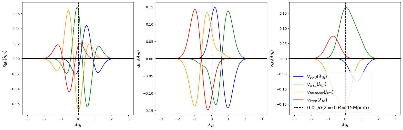
Figure 5: $s_{(E)}(\lambda_{\text{th}})$, $u_{(E)}(\lambda_{\text{th}})$ and $v_{(E)}(\lambda_{\text{th}})$ as a function of threshold, predicted by the Gram-Charlier development. Results are shown for the four different environments: void in blue, wall in green, filament in orange, and knot in red. The vertical black line is the threshold used in the paper.

References

• Aragón-Calvo et al. (2007a) Aragón-Calvo, M. A., Jones, B. J. T., van de Weygaert, R., & van der Hulst, J. M. 2007a, A&A, 474, 315
• Aragón-Calvo et al. (2010a) Aragón-Calvo, M. A., Platen, E., van de Weygaert, R., & Szalay, A. S. 2010a, ApJ, 723, 364
• Aragón-Calvo et al. (2010b) Aragón-Calvo, M. A., van de Weygaert, R., & Jones, B. J. T. 2010b, MNRAS, 408, 2163
• Aragón-Calvo et al. (2007b) Aragón-Calvo, M. A., van de Weygaert, R., Jones, B. J. T., & van der Hulst, J. M. 2007b, ApJ, 655, L5
• Arnold et al. (1982) Arnold, V. I., Shandarin, S. F., & Zeldovich, I. B. 1982, Geophysical and Astrophysical Fluid Dynamics, 20, 111
• Bernardeau et al. (2002) Bernardeau, F., Colombi, S., Gaztañaga, E., & Scoccimarro, R. 2002, Physics Reports, 367, 1–248
• Bond et al. (1996) Bond, J. R., Kofman, L., & Pogosyan, D. 1996, Nature, 380, 603
• Bonnaire et al. (2022) Bonnaire, T., Aghanim, N., Kuruvilla, J., & Decelle, A. 2022, A&A, 661, A146
• Carlesi et al. (2014) Carlesi, E., Knebe, A., Lewis, G. F., Wales, S., & Yepes, G. 2014, Monthly Notices of the Royal Astronomical Society, 439, 2943
• Codis et al. (2018a) Codis, S., Jindal, A., Chisari, N. E., et al. 2018a, MNRAS, 481, 4753
• Codis et al. (2012) Codis, S., Pichon, C., Devriendt, J., et al. 2012, MNRAS, 427, 3320
• Codis et al. (2013) Codis, S., Pichon, C., Pogosyan, D., Bernardeau, F., & Matsubara, T. 2013, MNRAS, 435, 531
• Codis et al. (2018b) Codis, S., Pogosyan, D., & Pichon, C. 2018b, MNRAS, 479, 973
• Colombi et al. (2000) Colombi, S., Pogosyan, D., & Souradeep, T. 2000, Phys. Rev. Lett., 85, 5515
• Cui et al. (2019) Cui, W., Knebe, A., Libeskind, N. I., et al. 2019, Monthly Notices of the Royal Astronomical Society
• Cui et al. (2017) Cui, W., Knebe, A., Yepes, G., et al. 2017, Monthly Notices of the Royal Astronomical Society, 473, 68–79
• de Lapparent et al. (1986) de Lapparent, V., Geller, M. J., & Huchra, J. P. 1986, ApJ, 302, L1
• Doroshkevich (1970) Doroshkevich, A. G. 1970, Astrophysics, 6, 320
• Falck et al. (2012) Falck, B. L., Neyrinck, M. C., & Szalay, A. S. 2012, ApJ, 754, 126
• Fisher et al. (2016) Fisher, J. D., Faltenbacher, A., & Johnson, M. S. T. 2016, Monthly Notices of the Royal Astronomical Society, 458, 1517
• Forero-Romero et al. (2009) Forero-Romero, J. E., Hoffman, Y., Gottlöber, S., Klypin, A., & Yepes, G. 2009, Monthly Notices of the Royal Astronomical Society, 396, 1815–1824
• Gay et al. (2012) Gay, C., Pichon, C., & Pogosyan, D. 2012, Physical Review D, 85
• Gott et al. (1987) Gott, III, J. R., Weinberg, D. H., & Melott, A. L. 1987, ApJ, 319, 1
• Hahn et al. (2007b) Hahn, O., Carollo, C. M., Porciani, C., & Dekel, A. 2007b, Monthly Notices of the Royal Astronomical Society, 381, 41
• Hahn et al. (2007a) Hahn, O., Porciani, C., Carollo, C. M., & Dekel, A. 2007a, Monthly Notices of the Royal Astronomical Society, 375, 489
• Hasan et al. (2023) Hasan, F., Burchett, J. N., Abeyta, A., et al. 2023, ApJ, 950, 114
• Hoffman et al. (2012) Hoffman, Y., Metuki, O., Yepes, G., et al. 2012, Monthly Notices of the Royal Astronomical Society, 425, 2049–2057
• Juszkiewicz et al. (1993) Juszkiewicz, R., Bouchet, F. R., & Colombi, S. 1993, The Astrophysical Journal, 412, L9
• Klypin & Shandarin (1983) Klypin, A. A. & Shandarin, S. F. 1983, MNRAS, 204, 891
• Kraljic et al. (2018) Kraljic, K., Arnouts, S., Pichon, C., et al. 2018, MNRAS, 474, 547
• Lee & Park (2009) Lee, J. & Park, D. 2009, ApJ, 696, L10
• Lewis et al. (2000) Lewis, A., Challinor, A., & Lasenby, A. 2000, ApJ, 538, 473
• Libeskind et al. (2013) Libeskind, N. I., Hoffman, Y., Forero-Romero, J., et al. 2013, MNRAS, 428, 2489
• Libeskind et al. (2017) Libeskind, N. I., van de Weygaert, R., Cautun, M., et al. 2017, Monthly Notices of the Royal Astronomical Society, 473, 1195–1217
• Lokas et al. (1995) Lokas, E. L., Juszkiewicz, R., Weinberg, D. H., & Bouchet, F. R. 1995, Monthly Notices of the Royal Astronomical Society, 274, 730
• Matsubara (2003) Matsubara, T. 2003, ApJ, 584, 1
• Metuki et al. (2015) Metuki, O., Libeskind, N. I., Hoffman, Y., Crain, R. A., & Theuns, T. 2015, MNRAS, 446, 1458
• Nuza et al. (2014) Nuza, S. E., Kitaura, F.-S., Heß, S., Libeskind, N. I., & Müller, V. 2014, MNRAS, 445, 988
• Peebles (1980) Peebles, P. J. E. 1980, The large-scale structure of the universe (Princeton University Press)
• Pogosyan et al. (2009) Pogosyan, D., Gay, C., & Pichon, C. 2009, Phys. Rev. D, 80, 081301
• Pogosyan et al. (2009) Pogosyan, D., Pichon, C., Gay, C., et al. 2009, MNRAS, 396, 635
• Poudel et al. (2017) Poudel, A., Heinämäki, P., Tempel, E., et al. 2017, A&A, 597, A86
• Regaldo-Saint Blancard et al. (2021) Regaldo-Saint Blancard, B., Codis, S., Bond, J. R., & Stein, G. 2021, MNRAS, 504, 1694
• Sousbie (2011) Sousbie, T. 2011, Monthly Notices of the Royal Astronomical Society, 414, 350
• Sousbie et al. (2009) Sousbie, T., Colombi, S., & Pichon, C. 2009, MNRAS, 393, 457
• Sousbie et al. (2008) Sousbie, T., Pichon, C., Colombi, S., Novikov, D., & Pogosyan, D. 2008, MNRAS, 383, 1655
• Suárez-Pérez et al. (2021) Suárez-Pérez, J. F., Camargo, Y., Li, X.-D., & Forero-Romero, J. E. 2021, The Astrophysical Journal, 922, 204
• Villaescusa-Navarro et al. (2020) Villaescusa-Navarro, F., Hahn, C., Massara, E., et al. 2020, ApJS, 250, 2
• Wang & Szalay (2014) Wang, X. & Szalay, A. 2014, arXiv e-prints, arXiv:1411.4117
• Wang et al. (2014) Wang, X., Szalay, A., Aragón-Calvo, M. A., Neyrinck, M. C., & Eyink, G. L. 2014, ApJ, 793, 58
• Zel’dovich (1970) Zel’dovich, Y. B. 1970, A&A, 5, 84