Localization of Dirac modes in the $\mathrm{SU}(2)$-Higgs model at finite temperature

Abstract

We investigate the connection between localization of low-lying Dirac modes and Polyakov-loop ordering in the lattice $\mathrm{SU}(2)$-Higgs model at finite temperature, probed with static external staggered fermions. After mapping out the phase diagram of the model at a fixed temporal extension in lattice units, we study the localization properties of the low-lying modes of the staggered Dirac operator, how these properties change across the various transitions, and how these modes correlate with the gauge and Higgs fields. We find localized low modes in the deconfined and in the Higgs phase, where the Polyakov loop is strongly ordered, but in both cases they disappear as one crosses over to the confined phase. Our findings confirm the general expectations of the “sea/islands” picture, and the more detailed expectations of its refined version concerning the favorable locations of localized modes, also in the presence of dynamical scalar matter.

I Introduction

Although it is well established that the finite-temperature QCD transition is an analytic crossover [1, 2], the microscopic mechanism that drives it is still being actively studied. The main goals of this line of research are a better understanding of the connection between deconfinement and restoration of chiral symmetry, both taking place in the crossover region; and of the fate of the anomalous $\mathrm{U}(1)_{A}$ symmetry, especially in the chiral limit. In this context, the fact that also the nature of the low-lying Dirac eigenmodes changes radically in the crossover region has aroused some interest. While delocalized in the low-temperature, confined and chirally broken phase, these modes become in fact spatially localized in the high-temperature, deconfined and (approximately) chirally restored phase, up to a critical point in the spectrum known as “mobility edge” [3, 4, 5, 6, 7, 8, 9] (see Ref. [10] for a recent review). As the strength of chiral symmetry breaking is controlled by the density of low-lying Dirac modes [11], while the change in their localization properties is mainly due to the ordering of the Polyakov loop in the high-temperature phase [12, 13, 14, 15, 10, 16], low-lying eigenmodes could provide the link between deconfinement and restoration of chiral symmetry.

The connection between low-mode localization and Polyakov-loop ordering is qualitatively explained by the “sea/islands” picture, initially proposed in Ref. [12], and further developed in Refs. [13, 14, 15, 10, 16]. In the deconfined phase, typical gauge configurations display a “sea” of ordered Polyakov loops, which on the one hand provides a spatially (approximately) uniform region where Dirac modes can easily delocalize, and on the other hand opens a (pseudo)gap in the near-zero spectrum. Polyakov-loop fluctuations away from order, and more generally gauge-field fluctuations with reduced correlation in the temporal direction, allow for eigenvalues below the gap; since in the deconfined phase these fluctuations typically form well separated “islands”, they tend to “trap” the low eigenmodes, causing their localization.

The sea/islands mechanism is quite general, and requires essentially only the ordering of the Polyakov loop for low-mode localization to take place . This leads one to expect localization of low Dirac modes to be a generic phenomenon in the deconfined phase of a gauge theory, an expectation so far fully confirmed by numerical results, both for pure gauge theories [18, 19, 20, 21, 22, 12, 23, 24, 25, 26, 27, 16] and in the presence of dynamical fermionic matter [28, 29]. An interesting aspect of the deconfinement/localization relation is that while the thermal transition can be a smooth, analytic crossover, the appearance of a mobility edge can only be sudden, taking place at a well-defined temperature. If the connection between deconfinement and localization is indeed general, one can then associate the (possibly smooth) thermal transition with a (definitely sharp) “geometric” transition (a similar suggestion, although in connection with deconfinement and center vortices, was made in Ref. [30], from which we borrowed the terminology). This point of view is supported by the fact that the geometric and the thermodynamic transition coincide when the latter is a genuine phase transition [23, 24, 25, 26, 27, 16, 28, 29].

As a further test of the universality of the sea/islands mechanism, one can investigate whether a change in the localization properties of low modes takes place across other thermal transitions where the Polyakov loop gets ordered, besides the usual deconfinement transition. As an example, Ref. [26] studied low-mode localization across the “reconfinement” transition in trace-deformed $\mathrm{SU}(3)$ gauge theory at finite temperature [31, 32, 33, 34, 35]. While localized modes are present in the deconfined phase also at nonzero deformation parameter, where the Polyakov-loop expectation value is different from zero, they disappear as the system reconfines and the Polyakov-loop expectation value vanishes.

Yet another test of universality consists in changing the type of dynamical matter from fermionic to scalar. As long as a phase with ordered Polyakov loops exists, this should not affect the expectations of the sea/islands picture, and localized modes should appear in the spectrum of the Dirac operator in that phase. In this context, the Dirac operator can be seen simply as a mathematical probe of certain properties of the gauge fields or, more physically, as a probe of how these fields couple to external, static (i.e., infinitely heavy) fermion fields.

A model allowing one to carry out both these tests at once is the lattice fixed-length $\mathrm{SU}(2)$-Higgs model [36]. At zero temperature the phase diagram of this model has been studied in depth both with analytical [36] and numerical [37, 38, 39, 40, 41, 42] methods. This model has two parameters, namely the (inverse) gauge coupling $\beta$ and the Higgs-gauge coupling $\kappa$, and it displays two lines of transitions in the $(\beta,\kappa)$ plane as follows [42]:

• a line of crossovers at $\beta\approx\beta_{\mathrm{bulk}}$, starting from the bulk transition (crossover) of the pure gauge $\mathrm{SU}(2)$ theory [43] at $(\beta,\kappa)=(\beta_{\mathrm{bulk}},0)$, and ending at some point $(\beta_{e},\kappa_{e})$;

• a line of crossovers coming down from large $\kappa$ at small $\beta$, meeting the first line at $(\beta_{e},\kappa_{e})$, turning into a line of first-order transitions at $(\beta_{f},\kappa_{f})$, and tending to $\kappa\approx 0.6$ as $\beta\to\infty$.

These transition lines separate three phases of the system: a confined phase at low $\beta$ and low $\kappa$; a deconfined phase at high $\beta$ and low $\kappa$; and a Higgs phase at high $\kappa$. A similar phase diagram was found at finite temperature, although the transition lines were all identified as crossovers in that case [42]. The absence of a sharp transition between the confined and the Higgs phase at any $\kappa$ at sufficiently low $\beta$ was proved in Ref. [36], where it was also shown that in this region all local correlation functions, and so the spectrum of the theory, depend analytically on the couplings.

While fermions are absent in the $\mathrm{SU}(2)$-Higgs model, one can still probe this system using static external fermions coupled to the $\mathrm{SU}(2)$ gauge field, as pointed out above. One can then study how the corresponding Dirac spectrum behaves, and check what happens to the localization properties of its low modes across the various transitions, in particular as one crosses over to the Higgs phase starting from either the confined or the deconfined phase. Since eigenvalues and eigenvectors of the Dirac operator are nonlocal functions of the gauge fields, they can display non-analytic behavior even in the strip of the $(\beta,\kappa)$ plane where all local correlators are analytic functions of the couplings, and so they could allow one to sharply distinguish the confined and the Higgs phase. (A different approach to this issue, based on the analogies between gauge-Higgs theories and spin glasses, is discussed in the review Ref. [44] and references therein.)

In this paper we study the spectrum and the eigenvectors of the staggered lattice Dirac operator in the $\mathrm{SU}(2)$-Higgs model at finite temperature. After briefly describing the model, in section II we introduce the tools we use to investigate the localization properties of staggered eigenmodes. In section III we map out the phase diagram of the model at finite temperature, working at fixed temporal extension in lattice units. In section IV we analyze the staggered eigenmodes, focussing in particular on how their localization properties change across the transitions between the confined, deconfined, and Higgs phases. We then study in detail the correlation between eigenmodes and the gauge and Higgs fields, to identify the field fluctuations mostly responsible for localization. Finally, in section V we draw our conclusions and show some prospects for the future.

II $\mathrm{SU}(2)$-Higgs model and localization

In this section we describe the fixed-length $\mathrm{SU}(2)$-Higgs model, and discuss how to characterize the localization properties of Dirac modes, and how these correlate with the gauge and Higgs fields.

II.1 $\mathrm{SU}(2)$-Higgs model on the lattice

We study the lattice $\mathrm{SU}(2)$-Higgs model in 3+1 dimensions, defined by the action

$$S=-\frac{\beta}{2}\sum_{n}\sum_{1\leq\mu<\nu\leq 4}{\rm tr}\,U_{\mu\nu}(n)-\frac{\kappa}{2}\sum_{n}\sum_{1\leq\mu\leq 4}{\rm tr}\,G_{\mu}(n)\,,$$ (1)

where we omitted an irrelevant additive constant. Here $n=(\vec{x},t)$, $n_{\mu}=0,\ldots,N_{\mu}-1$, are the sites of a hypercubic $N_{s}^{3}\times N_{t}$ lattice, i.e., $N_{1,2,3}=N_{s}$ and $N_{4}=N_{t}$, where $\mu=1,\ldots,4$ denotes the lattice directions and $\hat{\mu}$ the corresponding unit vectors. The dynamical variables are the $\mathrm{SU}(2)$ matrices $U_{\mu}(n)$ and $\phi(n)$, representing respectively the gauge variables associated with the link connecting $n$ and $n+\hat{\mu}$, and the unit-length Higgs field doublet (recast as a unitary matrix) associated with site $n$, and

$$U_{\mu\nu}(n) =U_{\mu}(n)U_{\nu}(n+\hat{\mu})U_{\mu}(n+\hat{\nu})^{\dagger}U_{\nu}(n)^{\dagger}\,,$$ (2)

$$G_{\mu}(n) =\phi(n)^{\dagger}U_{\mu}(n)\phi(n+\hat{\mu})\,,$$

are the plaquette variables associated with the elementary lattice squares, and the nontrivial part of the discretized covariant derivative of the Higgs field, which we will refer to as the Higgs-gauge field coupling term. Periodic boundary conditions are imposed on $U_{\mu}(n)$ and $\phi(n)$ in all directions. In what follows we will also make use of the Polyakov loop winding around the temporal direction,

$$P(\vec{x})={\rm tr}\,\prod_{t=0}^{N_{t}-1}U_{4}(\vec{x},t)\,.$$ (3)

Expectation values are defined as

$$\langle O\rangle =\frac{1}{Z}\int DU\int D\phi\,e^{-S(U,\phi)}O(U,\phi)\,,$$ (4)

$$Z =\int DU\int D\phi\,e^{-S(U,\phi)}\,,$$

where $DU$ and $D\phi$ denote the products of the $\mathrm{SU}(2)$ Haar measures associated with $U_{\mu}(n)$ and $\phi(n)$.

We study this model at finite temperature $T=1/(aN_{t})$, where $a$ is the lattice spacing, which can be set by suitably tuning the parameters of the model, namely the inverse gauge coupling $\beta$ and the Higgs-gauge field coupling $\kappa$. However, since we are not interested here in taking the continuum limit, we treat the model simply as a two-parameter anisotropic statistical mechanics system, keeping $N_{t}$ fixed as we take the thermodynamic limit $N_{s}\to\infty$, and as we change $\beta$ and $\kappa$ freely. To study the phase diagram in the $(\beta,\kappa)$ plane we use the average plaquette, Polyakov loop, and Higgs-gauge field coupling term,

$$\langle U\rangle =\frac{1}{N_{t}V}\sum_{n}\left\langle U(n)\right\rangle\,, \langle P\rangle =\frac{1}{V}\sum_{\vec{x}}\left\langle P(\vec{x})\right\rangle\,,$$ (5)

$$\langle G\rangle =\frac{1}{N_{t}V}\sum_{n}\left\langle G(n)\right\rangle\,,$$

where $V=N_{s}^{3}$ is the lattice volume, and the corresponding susceptibilities,

$$\chi_{U} =\frac{1}{N_{t}V}\left(\left\langle\left({\textstyle\sum_{n}}U(n)\right)^{2}\right\rangle-\left\langle{\textstyle\sum_{n}}U(n)\rule{0.0pt}{12.0pt}\right\rangle^{2}\right)\,,$$ (6)

$$\chi_{P} =\frac{1}{V}\left(\left\langle\left({\textstyle\sum_{\vec{x}}}\,{\rm tr}\,P(\vec{x})\right)^{2}\right\rangle-\left\langle{\textstyle\sum_{\vec{x}}}\,{\rm tr}\,P(\vec{x})\rule{0.0pt}{12.0pt}\right\rangle^{2}\right)\,,$$

$$\chi_{G} =\frac{1}{N_{t}V}\left(\left\langle\left({\textstyle\sum_{n}}G(n)\right)^{2}\right\rangle-\left\langle{\textstyle\sum_{n}}{\rm tr}\,G(n)\rule{0.0pt}{12.0pt}\right\rangle^{2}\right)\,.$$

In Eqs. (5) and (6) we denoted with $U(n)$ and $G(n)$ the average plaquette and gauge-Higgs coupling term touching a lattice site $n$,

$$U(n) =\frac{1}{24}\sum_{1\leq\mu<\nu\leq 4}{\rm tr}\,(U_{\mu\nu}(n)+U_{\mu\nu}(n-\hat{\mu})$$ (7)

$$\phantom{\frac{1}{24}\sum_{1\leq\mu<\nu\leq 4}}+U_{\mu\nu}(n-\hat{\nu})+U_{\mu\nu}(n-\hat{\mu}-\hat{\nu}))\,,$$

$$G(n) =\frac{1}{8}\sum_{1\leq\mu\leq 4}{\rm tr}\,(G_{\mu}(n)+G_{\mu}(n-\hat{\mu}))\,.$$

II.2 Localization of staggered eigenmodes

We are interested in the spectrum of the staggered Dirac operator in the background of the $\mathrm{SU}(2)$ gauge fields for fermions in the fundamental representation,

$$D^{\mathrm{stag}}=\frac{1}{2}\sum_{\mu}\eta_{\mu}(U_{\mu}{\rm T}_{\mu}-{\rm T}_{\mu}^{\dagger}U_{\mu}^{\dagger})\,,$$ (8)

where $\eta_{\mu}$ are the usual staggered phases and ${\rm T}_{\mu}$ are the translation operators with periodic (resp. antiperiodic) boundary conditions in space (resp. time), i.e.,

$$\eta_{\mu}(n) =(-1)^{\sum_{\alpha<\mu}n_{\alpha}}\,,$$ (9)

$$({\rm T}_{\mu})_{n,n^{\prime}} =b_{\mu}(n_{\mu})\delta_{n_{\mu}+1,n_{\mu}^{\prime}}\prod_{\alpha\neq\mu}\delta_{n_{\alpha},n_{\alpha}^{\prime}}\,,$$

with $n_{\mu}=N_{\mu}$ identified with $n_{\mu}=0$, and $b_{\mu}(n_{\mu})=1$, $\forall\mu,n_{\mu}$, except for $b_{4}(N_{t}-1)=-1$. Since the staggered operator is anti-Hermitian and anticommutes with $\varepsilon(n)=(-1)^{\sum_{\alpha}n_{\alpha}}$, its spectrum is purely imaginary and symmetric about the origin. We write

$$D^{\mathrm{stag}}\psi_{l}(n)=i\lambda_{l}\psi_{l}(n)\,,\qquad\lambda_{l}\in\mathbb{R}\,,$$ (10)

with eigenvectors $\psi_{l}(n)$ carrying an internal “color” index, $\psi_{l,c}(n)$, $c=1,2$, that has been suppressed for simplicity, and focus on $\lambda_{l}\geq 0$ only. Notice that since $\sigma_{2}U_{\mu}(n)\sigma_{2}=U_{\mu}(n)^{*}$, $D^{\mathrm{stag}}$ commutes with the antiunitary “time-reversal” operator $T=\sigma_{2}K$, where $K$ denotes complex conjugation. Since $T^{2}=-\mathbf{1}$, $D^{\mathrm{stag}}$ displays in this case doubly degenerate eigenvalues, and belongs to the symplectic class in the symmetry classification of random matrices [45, 46]. In the following it is understood that we work with the reduced spectrum, including only one eigenvalue from each degenerate pair.

Participation ratio

The localization properties of the staggered eigenmodes can be studied directly by looking at the eigenvectors, or indirectly by looking at the corresponding eigenvalues. In the first case one can study the volume scaling of the so-called participation ratio (PR) of the modes,

$$\mathrm{PR}_{l}=\frac{1}{N_{t}V}\mathrm{IPR}_{l}^{-1}\,,\qquad\mathrm{IPR}_{l}=\sum_{n}\|\psi_{l}(n)\|^{4}\,,$$ (11)

where $\|\psi_{l}(n)\|^{2}=\sum_{c=1}^{2}|\psi_{l,c}(n)|^{2}$, modes are normalized to 1, $\sum_{n}\|\psi_{l}(n)\|^{2}=1$, and IPR is the inverse participation ratio. The quantity $\mathrm{PR}_{l}$ measures the fraction of lattice volume $N_{t}V$ occupied by a given mode, and similarly $N_{t}V\cdot\mathrm{PR}_{l}=\mathrm{IPR}_{l}^{-1}$ gives the “mode size”. After averaging over an infinitesimally small spectral bin around a point $\lambda$ in the spectrum and over gauge configurations, as the spatial size $N_{s}$ grows the resulting average $\mathrm{PR}(\lambda,N_{s})$ tends to a constant if modes near $\lambda$ are delocalized on the entire lattice, and goes to zero as the inverse of the lattice volume if they are localized in a finite region. Equivalently, the similarly averaged mode size diverges linearly in the lattice volume for delocalized modes and tends to a constant for localized modes. In this paper we denote the average of any observable $O_{l}$ associated with mode $l$, following the procedure described above, as

$$O(\lambda,N_{s})=\frac{\left\langle\sum_{l}\delta(\lambda-\lambda_{l})O_{l}\right\rangle}{\left\langle\sum_{l}\delta(\lambda-\lambda_{l})\right\rangle}\,,$$ (12)

having made explicit the dependence on the spatial size of the lattice. The volume scaling of $\mathrm{PR}(\lambda,N_{s})$ defines the fractal dimension of modes in the neighborhood of $\lambda$,

$$\alpha(\lambda)=3+\lim_{N_{s}\to\infty}\frac{\log\mathrm{PR}(\lambda,N_{s})}{\log N_{s}}\,.$$ (13)

The multifractal properties of eigenmodes can be investigated by looking at the generalized inverse participation ratios,

$$(\mathrm{IPR}_{q})_{l}=\sum_{n}\|\psi_{l}(n)\|^{2q}\,,$$ (14)

with $(\mathrm{IPR}_{2})_{l}=\mathrm{IPR}_{l}$ . Their average according to Eq. (12) scales with the system size as $\mathrm{IPR}_{q}(\lambda,N_{s})\propto N_{s}^{-D_{q}(\lambda)(q-1)}$, with generalized fractal dimensions $D_{q}$ (notice $D_{2}=\alpha$). One has $D_{q}=3$ for delocalized modes and $D_{q}=0$ for localized modes, while a nontrivial $D_{q}$ signals eigenmode multifractality [48].

Spectral statistics

The localization properties of the eigenmodes reflect on the statistical properties of the eigenvalues [49]: for localized modes one expects independent fluctuations of the eigenvalues, while for delocalized modes one expects to find the correlations typical of dense random matrix models. It is convenient in this context to study the probability distribution of the so-called unfolded level spacings [45, 46],

$$s_{l}=\frac{\lambda_{l+1}-\lambda_{l}}{\langle\lambda_{l+1}-\lambda_{l}\rangle_{\lambda}}\,,$$ (15)

computed locally in the spectrum, i.e.,

$$p(s;\lambda,N_{s})=\frac{\left\langle\sum_{l}\delta(\lambda-\lambda_{l})\delta(s-s_{l})\right\rangle}{\left\langle\sum_{l}\delta(\lambda-\lambda_{l})\right\rangle}\,.$$ (16)

In Eq. (15), $\langle\lambda_{l+1}-\lambda_{l}\rangle_{\lambda}$ denotes the average spacing in the relevant spectral region, which for large volumes equals $\langle\lambda_{l+1}-\lambda_{l}\rangle_{\lambda}\to\frac{1}{N_{t}V\rho(\lambda)}$, where $\rho(\lambda)$ is the spectral density,

$$\rho(\lambda)=\lim_{V\to\infty}\frac{1}{N_{t}V}\left\langle{\textstyle\sum_{l}}\delta(\lambda-\lambda_{l})\right\rangle\,.$$ (17)

The statistical properties of the unfolded spacings are expected to be universal [45], i.e., independent of the details of the model, and can be compared to the theoretical predictions obtained from exactly solvable models. As the system size increases, for localized modes $p(s;\lambda,N_{s})$ should approach the exponential distribution, $p_{\mathrm{P}}(s)=e^{-s}$, appropriate for independent eigenvalues obeying Poisson statistics [45]. For delocalized modes $p(s;\lambda,N_{s})$ should instead approach the distribution $p_{\mathrm{RMT}}(s)$ predicted by the appropriate Gaussian Ensemble of Random Matrix Theory, which is the Gaussian Symplectic Ensemble in the case at hand [45, 46]. This quantity is known exactly, but is not available in closed form. An accurate approximation is provided by the symplectic Wigner surmise,

$$p_{\mathrm{WS}}(s)=\left(\frac{64}{9\pi}\right)^{3}s^{4}e^{-\frac{64}{9\pi}s^{2}}\,.$$ (18)

Mobility edge

Localized and delocalized modes are generally found in disjoint spectral regions separated by critical points known as mobility edges, where the localization length diverges and the system undergoes a phase transition along the spectrum, known as Anderson transition [48]. At the mobility edge the critical eigenmodes display a fractal dimension different from those of localized or delocalized modes, as well as a rich multifractal structure. This is reflected in critical spectral statistics different from both Poisson and RMT statistics. To monitor how the localization properties change along the spectrum using its statistical properties, it is convenient to use the integrated unfolded level spacing distribution,

$$I_{s_{0}}(\lambda,N_{s})=\int_{0}^{s_{0}}ds\,p(s;\lambda,N_{s})\,,$$ (19)

where $s_{0}\simeq 0.563$ is chosen so to maximize the difference between the expectations for Poisson and RMT distributions, $I_{s_{0},\mathrm{P}}\simeq 0.431$ and $I_{s_{0},\mathrm{RMT}}\simeq 0.0797$, estimated using $p_{\mathrm{P}}$ and $p_{\mathrm{WS}}$, see Eq. (18) above. This quantity allows one to determine the mobility edge very accurately by means of a finite-size-scaling analysis [50]. In fact, as the system size increases $I_{s_{0}}(\lambda,N_{s})$ tends to $I_{s_{0},\mathrm{P}}$ or $I_{s_{0},\mathrm{RMT}}$ depending on the localization properties of the modes in the given spectral region, except at the mobility edge where it is volume-independent and takes the value $I_{s_{0},c}$ corresponding to the critical statistics. This, however, requires large-scale simulations to achieve a sufficient quality of the data, and several large volumes.

One can give up some of the accuracy but save a lot in computing effort by using the critical value of the spectral statistic, expected to be universal, to determine the mobility edge simply by looking for the point where the curve for $I_{s_{0}}$ crosses its critical value, $I_{s_{0},c}$ (see, e.g, Refs. [28, 23, 25, 29]). This critical value is not known for the symplectic class, but it can be determined by identifying the scale-invariant point in the spectrum at some point in the parameter space of the model under study (if one can find an Anderson transition, of course); the corresponding critical value can then be used in the rest of the analysis. Notice that one could estimate the mobility edge in a finite volume as the point where $I_{s_{0}}$ takes any chosen value intermediate between the RMT and the Poisson predictions, and this would converge to the correct value in the infinite-volume limit. In this respect, the choice of $I_{s_{0},c}$ is only the most convenient, as it is expected to minimize the magnitude of finite-size effects.

Correlation with bosonic observables

To investigate the correlation between staggered eigenmodes and gauge and Higgs fields we considered the following observables,

$$\mathcal{U}_{l} =\sum_{n}U(n)\|\psi_{l}(n)\|^{2}\,, \mathcal{P}_{l} =\sum_{t,\vec{x}}P(\vec{x})\|\psi_{l}(\vec{x},t)\|^{2}\,,$$ (20)

$$\mathcal{G}_{l} =\sum_{n}G(n)\|\psi_{l}(n)\|^{2}\,,$$

averaged according to Eq. (12). Recall that $U(n)$ and $G(n)$ are the average plaquette and gauge-Higgs coupling term touching a lattice site $n$, defined in Eq. (7). For delocalized modes $\|\psi_{l}\|^{2}\sim\frac{1}{V}$, and the averages $\mathcal{U}(\lambda,N_{s})$, $\mathcal{P}(\lambda,N_{s})$, and $\mathcal{G}(\lambda,N_{s})$ of the observables in Eq. (20) are approximately equal to the average of the corresponding bosonic observable, i.e., $\langle U\rangle$, $\langle P\rangle$, and $\langle G\rangle$, respectively [see Eq. (5)]. For localized modes $\|\psi_{l}\|^{2}$ is non-negligible only inside a region of finite spatial volume, so $\mathcal{P}(\lambda,N_{s})$ measures the average Polyakov loop inside the localization region, and $\mathcal{U}(\lambda,N_{s})$ and $\mathcal{G}(\lambda,N_{s})$ measure respectively the average plaquette and gauge-Higgs coupling term in a neighborhood of the localization region. One should, however, keep in mind that there are 24 neighboring squares and 8 neighboring links to each site, so that a possible correlation of modes with the plaquette and gauge-Higgs coupling term fluctuations get diluted.

More informative than the averages of the observables in Eq. (20) are the corresponding centered and rescaled averages,

$$\widehat{\mathcal{U}}(\lambda,N_{s}) =\frac{\mathcal{U}(\lambda,N_{s})-\langle U\rangle}{\delta U}\,,$$ (21)

$$(\delta U)^{2} =\langle U(n)^{2}\rangle-\langle U(n)\rangle^{2}\,,$$

$$\widehat{\mathcal{P}}(\lambda,N_{s}) =\frac{\mathcal{P}(\lambda,N_{s})-\langle P\rangle}{\delta P}\,,$$

$$(\delta P)^{2} =\langle P(\vec{x})^{2}\rangle-\langle P(\vec{x})\rangle^{2}\,,$$

$$\widehat{\mathcal{G}}(\lambda,N_{s}) =\frac{\mathcal{G}(\lambda,N_{s})-\langle G\rangle}{\delta G}\,,$$

$$(\delta G)^{2} =\langle G(n)^{2}\rangle-\langle G(n)\rangle^{2}\,.$$

These quantities measure the correlation of the eigenmodes with fluctuations in the gauge and Higgs fields, normalized by the average size of these fluctuations. Indeed, writing these quantities out explicitly, one has, e.g.,

$$\widehat{\mathcal{U}}(\lambda,N_{s})=\left\langle{\textstyle\sum_{n}}\frac{{\textstyle\sum_{l}}\delta(\lambda-\lambda_{l})\|\psi_{l}(n)\|^{2}}{N_{t}V\rho(\lambda)}\,\frac{U(n)-\langle U\rangle}{\delta U}\right\rangle\,.$$ (22)

As a consequence, the observables in Eq. (21) vanish in the absence of correlation, and are strongly suppressed for delocalized modes. The normalization factor takes into account that for observables with a strongly peaked probability distribution even a correlation with small deviations from average is significant, indicating that eigenmodes are attracted by the corresponding type of fluctuations, and favor the locations where they show up in a field configuration. In particular, for localized modes this allows one to identify the most favorable type of fluctuations for localization.

Sea/islands picture

We also study the correlation between eigenmodes and the “islands” of the refined “sea/islands” picture of localization discussed in Ref. [16]. These are defined using the “Dirac-Anderson Hamiltonian” representation of the staggered Dirac operator [14], obtained by diagonalizing the temporal hopping term in $D^{\mathrm{stag}}$ [i.e., the term with $\mu=4$ in the sum in Eq. (8)] by means of a unitary transformation $\Omega$ [16],

$$H^{\mathrm{DA}}\equiv\Omega^{\dagger}(-iD^{\mathrm{stag}})\Omega=\mathcal{E}\mathbf{1}_{s}+\frac{1}{2i}\sum_{j=1}^{3}\eta_{j}({\cal V}_{j}{\rm T}_{j}-{\rm T}_{j}^{\dagger}{\cal V}_{j}^{\dagger})\,,$$ (23)

where $\mathbf{1}_{s}$ is the $V\times V$ identity matrix $(\mathbf{1}_{s})_{\vec{x},\vec{y}}=\delta_{\vec{x},\vec{y}}$, ${\rm T}_{j}$ are here the spatial translation operators $({\rm T}_{j})_{\vec{x},\vec{y}}=\delta_{\vec{x}+\hat{\jmath},\vec{y}}$ (with periodic boundary conditions understood), $\mathcal{E}$ is an $\vec{x}$-dependent $2N_{t}\times 2N_{t}$ diagonal matrix,

$$\mathcal{E}(\vec{x})_{ka\,lb} =\delta_{kl}\delta_{ab}e_{ka}(\vec{x})\,, e_{ka}(\vec{x}) =\eta_{4}(\vec{x})\sin\omega_{ka}(\vec{x})\,,$$ (24)

and ${\cal V}_{j}$ are $\vec{x}$-dependent $2N_{t}\times 2N_{t}$ unitary matrices,

$${\cal V}_{j}(\vec{x})_{ka\,lb} =\frac{1}{N_{t}}\sum_{t=0}^{N_{t}-1}e^{-i\left(\omega_{ka}(\vec{x})-\omega_{lb}(\vec{x}+\hat{\jmath})\right)t}\,U_{j}^{\rm tdg}(\vec{x},t)_{ab}\,,$$ (25)

with $k,l=0,\ldots N_{t}-1$ and $a,b=1,2$. Here “tdg” stands for “temporal diagonal gauge”, i.e., $U_{j}^{\rm tdg}$ are the spatial links in the temporal gauge where all Polyakov loops are diagonal ,

$$U_{j}^{\rm tdg}(\vec{x},t) =u(\vec{x})^{\dagger}P(\vec{x},t)U_{j}(\vec{x},t)P(\vec{x}+\hat{\jmath},t)^{\dagger}u(\vec{x}+\hat{\jmath})\,,$$ (26)

$$P(\vec{x},t+1) =P(\vec{x},t)U_{4}(\vec{x},t)\,,$$

with $P(\vec{x},0)=\mathbf{1}$, and $u(\vec{x})$ a suitable unitary matrix such that [notice $P(\vec{x})=P(\vec{x},N_{t})$]

$$P(\vec{x})=u(\vec{x})\mathrm{diag}(e^{i\phi_{1}(\vec{x})},e^{i\phi_{2}(\vec{x})})u(\vec{x})^{\dagger}\,,$$ (27)

with $\phi_{1,2}(\vec{x})\in[-\pi,\pi)$ and $e^{i\left(\phi_{1}(\vec{x})+\phi_{2}(\vec{x})\right)}=1$. Moreover, $\omega_{ka}(\vec{x})$ are effective Matsubara frequencies,

$$\omega_{ka}(\vec{x})=\frac{\phi_{a}(\vec{x})+(2n_{ka}+1)\pi}{N_{t}}\,,$$ (28)

with $n_{ka}\in\{0,\ldots,N_{t}-1\}$ chosen for each $a$ so that the “energies” $e_{ka}$ satisfy $0\leq e_{1a}(\vec{x})\leq e_{2a}(\vec{x})\leq\ldots\leq e_{\frac{N_{t}}{2}-1\,a}$, and $e_{k+\frac{N_{t}}{2}\,a}(\vec{x})=-e_{ka}(\vec{x})$, for $k=0,\ldots\frac{N_{t}}{2}-1$. Notice that thanks to the simple relation between $\phi_{1}$ and $\phi_{2}$, one has $e_{k1}=e_{k2}$. This double degeneracy is a consequence of the temporal hopping term being invariant under the time-reversal transformation $T$ (see section II.2). With this choice for $e_{ka}$, $H^{\mathrm{DA}}$ has the general structure

$$H^{\mathrm{DA}} =\begin{pmatrix}E&\mathbf{0}\\ \mathbf{0}&-E\end{pmatrix}$$ (29)

$$\phantom{=}+\frac{1}{2i}\sum_{j=1}^{3}\eta_{j}\left[\begin{pmatrix}A_{j}&B_{j}\\ B_{j}&A_{j}\end{pmatrix}{\rm T}_{j}-{\rm T}_{j}{}^{\dagger}\begin{pmatrix}A_{j}{}^{\dagger}&B_{j}{}^{\dagger}\\ B_{j}{}^{\dagger}&A_{j}{}^{\dagger}\end{pmatrix}\right]\,,$$

where $E,A_{j},B_{j}$ are $N_{t}\times N_{t}$ matrices.

It was argued in Ref. [16] that sites where the diagonal blocks $A_{j}$ are larger are the most favorable for the localization of low modes in a phase where the Polyakov loops are ordered. In general, spatial regions with larger $A_{j}$, which correspond to lower correlation among spatial links on different time slices, are expected to be favored by low modes; in an ordered phase such regions are localized, and so lead to low-mode localization. One can check this by looking at the correlation between modes and the quantity

$$A(\vec{x})=\frac{1}{6N_{t}}\sum_{j=1}^{3}{\rm tr}\,A_{j}(\vec{x})^{\dagger}A_{j}(\vec{x})+{\rm tr}\,A_{j}(\vec{x}-\hat{\jmath})^{\dagger}A_{j}(\vec{x}-\hat{\jmath})\,,$$ (30)

i.e., using the observable

$$\mathcal{A}_{l}=\sum_{\vec{x}}A(\vec{x})\sum_{t=0}^{N_{t}-1}\|\psi_{l}(\vec{x},t)\|^{2}\,,$$ (31)

averaged according to Eq. (12) to get $\mathcal{A}(\lambda,N_{s})$, and centered and rescaled according to Eq. (22) to get $\widehat{\mathcal{A}}(\lambda,N_{s})$, i.e.,

$$\widehat{\mathcal{A}}(\lambda,N_{s}) =\frac{\mathcal{A}(\lambda,N_{s})-\langle A\rangle}{\delta A}\,,$$ (32)

$$(\delta A)^{2} =\langle A(\vec{x})^{2}\rangle-\langle A(\vec{x})\rangle^{2}\,.$$

III Phase diagram at finite temperature

In this section we report our results on the phase diagram of the model. We worked at finite temperature, fixing the lattice temporal extension to $N_{t}=4$, and performing numerical simulations with a standard heatbath algorithm.

Theoretical arguments [36] and previous numerical studies [42] lead us to expect three phases: a confined phase at small $\beta$ and small $\kappa$; a deconfined phase at large $\beta$ and small $\kappa$; and a Higgs phase at large $\kappa$. Based on the finite-temperature results of Ref. [42], and on the observed weakening of the transition for smaller temporal extensions reported there, we expect that the transitions between the three phases are analytic crossovers. A detailed study of this issue is beyond the scope of this paper, so we limited most of our simulations to a single lattice volume with $N_{s}=20$, for 784 different $(\beta,\kappa)$ pairs, using 3000 configurations at each point. We took $\kappa\in[0,1.35]$ in steps of $\Delta\kappa=0.05$ and $\beta\in[1.5,2.85]$ in steps of $\Delta\beta=0.05$. A detailed volume-scaling study was done on a subset of these points: we discuss this below.

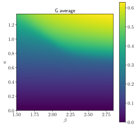
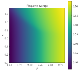
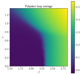
Figure 1: Heatmap plot of the expectation value of $G$ (top panel), $U$ (center panel), and $P$ (bottom panel), see Eq. (5). Here $N_{s}=20$ and $N_{t}=4$.

We show our results for $\langle G\rangle$, $\langle U\rangle$, and $\langle P\rangle$ in Fig. 1 as heatmap plots, obtained by cubic interpolation of the numerical results at the simulation points. These confirm our expectations, and allow us to characterize the confined phase at small $\beta$ and $\kappa$ by small $\langle G\rangle$, $\langle U\rangle$, and $\langle P\rangle$; the deconfined phase at large $\beta$ and small $\kappa$ by small $\langle G\rangle$ and large $\langle U\rangle$ and $\langle P\rangle$; and the Higgs phase at large $\kappa$ by large $\langle G\rangle$, $\langle U\rangle$, and $\langle P\rangle$. We estimated errors with a standard jackknife procedure: they are not shown, but relative errors are always within $7\cdot 10^{-5}$ for $\langle U\rangle$; $2\cdot 10^{-3}$ for $\langle G\rangle$; and within $1\cdot 10^{-3}$ for $\langle P\rangle$, except deep inside the confined phase where the average becomes very small and indistinguishable from zero within errors. More precisely, the expectation value of the gauge-Higgs coupling term (Fig. 1, top panel) divides the phase diagram into two pieces: the Higgs phase at large $\kappa$, with large $\langle G\rangle$, and the (undivided) confined and deconfined phases at small $\kappa$, with similar and small values of $\langle G\rangle$. The expectation value of the plaquette and of the Polyakov loop (Fig. 1, center and bottom panel) divide the phase diagram into two parts in a different way: the confined phase at low $\beta$ and $\kappa$, where both $\langle U\rangle$ and $\langle P\rangle$ are small, and the (undivided) Higgs and deconfined phases, where both $\langle U\rangle$ and $\langle P\rangle$ are large.

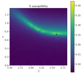
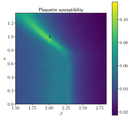
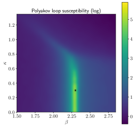
Figure 2: Heatmap plot of the susceptibility $\chi_{G}$ of the gauge-Higgs coupling term $G$ (top panel), the plaquette susceptibility $\chi_{U}$ (center panel), and the logarithm of the Polyakov-loop susceptibility $\chi_{P}$ (bottom panel), see Eqs. (5) and (6). Here $N_{s}=20$ and $N_{t}=4$. In the top panel, the black point shows where the mobility edge $\lambda_{c}=\lambda_{c}(\kappa)$ has an inflection point along the line at constant $\beta=2.6$, see Fig. 17. In the center panel, it shows where the mobility edge $\lambda_{c}=\lambda_{c}(\beta)$ vanishes along the line at constant $\kappa=1.0$, see Fig. 16. In the bottom panel, it shows where the mobility edge $\lambda_{c}=\lambda_{c}(\beta)$ vanishes along the line at constant $\kappa=0.3$, see Fig. 15.

We show our results for the corresponding susceptibilities as heatmap plots in Fig. 2. Also in this case we estimated errors (not shown in the figure) with a standard jackknife procedure, finding them to be always within 3%. In the top panel we show our results for $\chi_{G}$. This quantity has a narrow ridge, visualized here as a bright line, providing a clear separation between the Higgs phase and the rest in most of the explored parameter space; a weakening of the transition is visible in the top left part of the phase diagram. In the center panel we show the plaquette susceptibility $\chi_{U}$. This separates clearly the confined phase from the Higgs phase, while the ridge broadens at the transition between confined and deconfined phase (as well as in the top left part of the phase diagram). In the bottom panel we show the logarithm of the Polyakov-loop susceptibility. This plot shows a bright line of strong transitions separating the confined and deconfined phases. This line continues in the top left part of the plot, still clearly separating the confined and Higgs phases, but it is much dimmer there as the signal is two orders of magnitude weaker than at the transition from the confined to the deconfined phase (see Figs. 4, top and 5, top). At the transition between the deconfined and Higgs phase $\chi_{P}$ shows an inflection point instead of a peak (see Fig. 6), with a sizeable decrease in susceptibility corresponding here to a noticeable darkening of the plot.

A sketch of the resulting phase diagram is shown in Fig. 3, obtained by merging the various transition lines, defined by the peaks of the suceptibilities. The dashed line at low $\beta$ and large $\kappa$ signals a sizeable reduction in the strength of the transition there, as shown by all three observables. Except in this region, where they slighly deviate from each other, the transition lines between confined and Higgs phase obtained from the three different susceptibilities agree with each other, so we drew a single line. Similarly, the transition lines between confined and deconfined phase obtained from the plaquette and the Polyakov loop susceptibility agree with each other, so we drew a single line in this case as well.

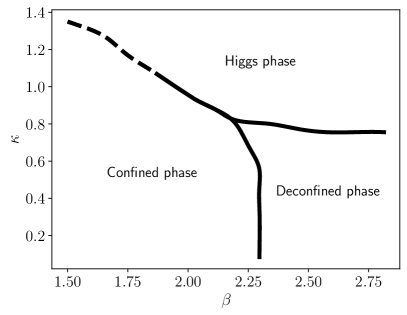
Figure 3: Schematic drawing of the phase diagram, obtained combining the maxima of the susceptibilities shown in Fig. 2. A dashed line is used to indicate the weakening of the transition.

To verify the expected crossover nature of the transitions, we studied the volume dependence of the various susceptibilities in detail on three lines, one at constant $\kappa=0.5$ and two at constant $\beta=2.0$ and $\beta=2.6$, using lattices with $N_{s}=22,28,34,40$. For each simulation point and each lattice volume we used 4500 configurations. We estimated errors by first averaging over configurations in blocks of size $b_{\mathrm{size}}$ and computing the standard jackknife error on the blocked ensemble, and then increasing $b_{\mathrm{size}}$ until the error stabilized. For our final estimates we used samples of size $b_{\mathrm{size}}=20$, except at $\kappa=0.5$ where we used $b_{\mathrm{size}}=50$, although this was really needed only around $\beta=2.3$. We show our results in Figs. 4–6.

In Fig. 4 we show $\chi_{P}$, $\chi_{U}$ and $\chi_{G}$ along a line of constant $\kappa=0.5$ across the transition from the confined to the deconfined phase. The signal is very strong in $\chi_{P}$, and a small peak is visible also in $\chi_{U}$. The location of these peaks is not far from the critical point $\beta_{c}\approx 2.3$ of the pure gauge theory at $\kappa=0$ [52, 53, 54, 55]. The relatively large error bars found for $N_{s}=22$ between $\beta=2.28$ and $\beta=2.31$, especially at $\beta=2.3$, are most likely a finite-size effect due to the vicinity of the critical point of the pure gauge theory, and are not observed on larger volumes. On the other hand, no peak is visible in $\chi_{G}$, which is constant within errors across the transition. This makes the gauge-Higgs coupling term $G$ unsuitable to detect this transition.

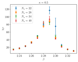
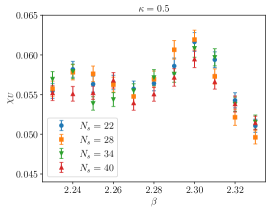
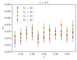
Figure 4: Polyakov-loop (top), plaquette (center), and gauge-Higgs coupling term (bottom) susceptibility across the transition between the confined and the deconfined phase at $\kappa=0.5$. Here $N_{t}=4$. The volume scaling is consistent with an analytic crossover.

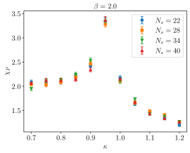
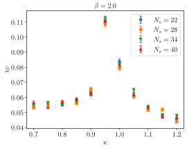
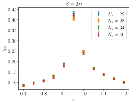
Figure 5: Polyakov-loop (top), plaquette (center), and gauge-Higgs coupling term (bottom) susceptibility near the transition between the confined and the Higgs phase at $\beta=2.0$. Here $N_{t}=4$. The volume scaling is consistent with an analytic crossover.

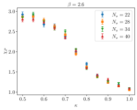
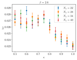
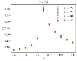
Figure 6: Polyakov-loop (top), plaquette (center), and gauge-Higgs coupling term (bottom) susceptibility near the transition between the deconfined and the Higgs phase at $\beta=2.6$. Here $N_{t}=4$. The volume scaling is consistent with an analytic crossover.

In Fig. 5 we show $\chi_{P}$, $\chi_{U}$ and $\chi_{G}$ along a line of constant $\beta=2.0$ across the transition from the confined to the Higgs phase. A clear peak is visible in all three observables, with $\chi_{P}$ two orders of magnitude smaller than in Fig. 4 (top), and $\chi_{U}$ a factor of 2 larger than in Fig. 4 (bottom).

Finally, in Fig. 6 we show $\chi_{P}$, $\chi_{U}$ and $\chi_{G}$ along a line of constant $\beta=2.6$ across the transition from the deconfined to the Higgs phase. We observe a peak in $\chi_{G}$, of similar magnitude as the one in Fig. 5 (bottom) for the transition from the confined to the Higgs phase. Neither $\chi_{U}$ nor $\chi_{P}$ show any significant peak: $\chi_{U}$ changes slope at the transition, while $\chi_{P}$ shows an inflection point. This makes $U$ and $P$ not quite suitable observables to detect this transition.

While these results do not logically exclude the possibility of genuine phase transitions at some points in the phase diagram, combined with the results of Ref. [42] they make it implausible.

IV Localization properties of Dirac eigenmodes

$(\beta=1.9,\kappa=1.0)$
$N_{s}$	#configurations	#eigenvalues
16	3000	33
20	1500	63

$(\beta=2.1,\kappa=1.0)$ and $(\beta=2.6,\kappa=0.3)$
$N_{s}$	#configurations	#eigenvalues
20	8970	63
24	8000	110
28	3000	174
32	1150	260

Table 1: Configuration statistics and number of (non-degenerate) eigenvalues used to study the volume scaling of the localization properties of staggered eigenmodes in the confined phase (top table) and in the deconfined and Higgs phases (bottom table).

In this section we discuss the localization properties of the eigenmodes of the staggered operator and how these correlate with the gauge and Higgs fields, and we present a detailed test of the sea/islands mechanism. We obtained the lowest modes of $D^{\textrm{stag}}$ using the PRIMME package [56, 57] for sparse matrices, exploiting Chebyshev acceleration for faster convergence. The use of algorithms for sparse matrices allows us to reduce the scaling of computational time from $N_{s}^{9}$, expected for full diagonalization, down to $N_{s}^{6}$.

We first analyzed the eigenmodes in detail at three points of the phase diagram, using several lattice volumes to study the scaling of eigenvector and eigenvalue observables with the system size. These points are $\beta=1.9,\kappa=1.0$, in the confined phase, right below the transition to the Higgs phase at constant $\kappa$ ($\beta/\beta_{c}\approx 0.97$, with $\beta_{c}\approx 1.95$ corresponding to the peak in the Polyakov-loop susceptibility); $\beta=2.1,\kappa=1.0$, in the Higgs phase, not far above the transition between the two phases ($\beta/\beta_{c}\approx 1.08$); and $\beta=2.6,\kappa=0.3$, deep in the deconfined phase. We looked at two lattice volumes in the confined phase, and at four lattice volumes in the deconfined and Higgs phases; see Tab. 1 for details about system size, configuration statistics, and number of eigenmodes. We then computed the relevant observables locally in the spectrum, approximating Eq. (12) by averaging over spectral bins of size $\Delta\lambda=0.0025$ at $\beta=1.9$, $\kappa=1.0$ (confined phase), $\Delta\lambda=0.01$ at $\beta=2.6$, $\kappa=0.3$ (deconfined phase), and $\Delta\lambda=0.0075$ at $\beta=2.1$, $\kappa=1.0$ (Higgs phase). Our results, reported in sections IV.1 and IV.2, demonstrate low-mode localization in the deconfined and in the Higgs phase.

This detailed study also allowed us to estimate the critical value of $I_{s_{0}}$, which we could then use to efficiently determine the dependence of the mobility edge, $\lambda_{c}$, on the parameters $\beta$ and $\kappa$. We did this on two lines at constant $\kappa$: one in the deconfined phase with $\kappa=0.3$, changing $\beta$ in the interval $[2.35,2.60]$ with increments $\Delta\beta=0.05$; and one in the Higgs phase with $\kappa=1.0$, changing $\beta$ in $[2.1,2.4]$ with increments $\Delta\beta=0.05$. We also studied one line at constant $\beta=2.6$, changing $\kappa$ in $[0.35,1.0]$ in increments of $\Delta\kappa=0.05$. Here we used a single volume ($N_{s}=20,N_{t}=4$) and 3000 configurations at each point (except for the three points already discussed above). In all these calculations we computed $I_{s_{0}}$ locally in the spectrum averaging over bins of size $\Delta\lambda=0.008$. Our results, reported in section IV.3, show that along both lines at constant $\kappa$ the mobility edge disappears at a critical $\beta$ near the crossover to the confined phase; and that along the line at constant $\beta$ the mobility edge is always nonzero, but it changes behavior at the crossover between the deconfined and the Higgs phase.

We then studied the correlation between localized modes and the fluctuations of the gauge and Higgs fields, and tested the refined sea/islands picture of Ref. [16]. Our results, reported in section IV.4, show a strong correlation with Polyakov-loop and plaquette fluctuations, and an even stronger correlation with the fluctuations identified in Ref. [16] as the most relevant to localization.

IV.1 Eigenvector observables

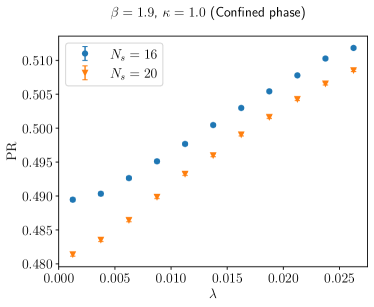
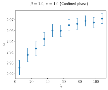
Figure 7: Participation ratio, Eq. (11), of the low staggered eigenmodes at $\beta=1.9$ and $\kappa=1.0$ in the confined phase for two different spatial volumes (top panel) and corresponding fractal dimension estimated using Eq. (33) with $N_{s_{1}}=16$, $N_{s_{2}}=20$ (bottom panel). Here $N_{t}=4$.

In the top panel of Fig. 7 we show the PR of the modes in the confined phase. The PR is slightly larger for $N_{s}=16$ than for $N_{s}=20$, signaling that the fractal dimension is smaller than 3. This is shown explicitly in the bottom panel, where we plot $\alpha(\lambda)$, see Eq. (13). This is estimated numerically from a pair of volumes as

$$\alpha_{\mathrm{num}}(\lambda;N_{s1},N_{s2})=3+\frac{\log\frac{\mathrm{PR}(\lambda,N_{s1})}{\mathrm{PR}(\lambda,N_{s2})}}{\log\frac{N_{s1}}{N_{s2}}}\,.$$ (33)

The fractal dimension of near-zero modes is slightly below 3, and approaches 3 as one moves up in the spectrum. Taken at face value, this means that these modes are only slightly short of being fully delocalized. Clearly, this effect could be just a finite-size artifact due to the small volumes employed here. However, it could also signal that a “geometric” transition is approaching, where a mobility edge and, correspondingly, critical modes appear at the origin.

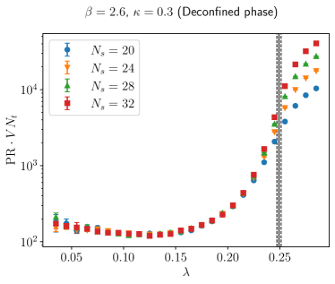
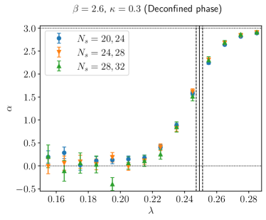
Figure 8: The mode size $N_{t}V\cdot\mathrm{PR}=\mathrm{IPR}^{-1}$, Eq. (11), of the low staggered eigenmodes for different volumes (top panel), and corresponding fractal dimension estimated using Eq. (33) with three different volume pairs (bottom panel), at $\beta=2.6$ and $\kappa=0.3$ in the deconfined phase. Here $N_{t}=4$. The vertical solid line shows the position of the mobility edge, vertical dashed lines indicate the corresponding error band. In the bottom panel, horizontal dotted lines mark the values $\alpha=0$, corresponding to localized modes, and $\alpha=3$, corresponding to totally delocalized modes.

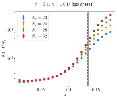
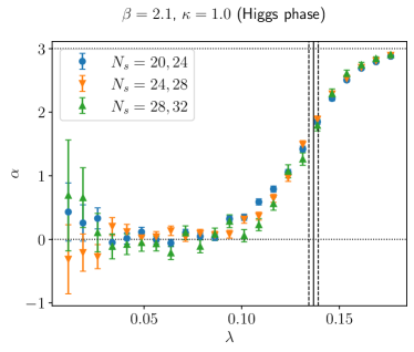
Figure 9: As in Fig. 8, but at $\beta=2.1$ and $\kappa=1.0$ in the Higgs phase.

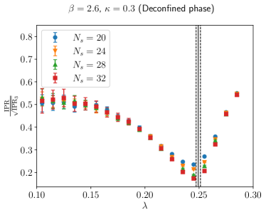
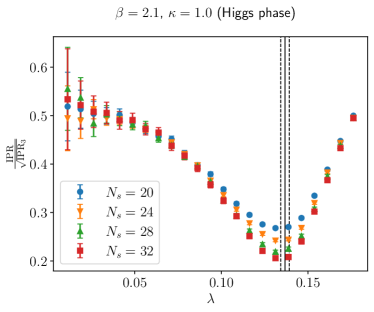
Figure 10: Ratio of generalized IPRs, Eq. (34), at $\beta=2.6$ and $\kappa=0.3$ in the deconfined phase (top panel), and at $\beta=2.1$ and $\kappa=1.0$ in the Higgs phase (bottom panel). The vertical solid line shows the position of the mobility edge, vertical dashed lines indicate the corresponding error band. A nontrivial volume scaling indicates nontrivial multifractal properties of the eigenmodes at the mobility edge.

In the top panels of Figs. 8 and 9 we show the size $N_{t}V\cdot\mathrm{PR}=\mathrm{IPR}^{-1}$ of the modes in the deconfined and in the Higgs phase, respectively. In both cases the size of the lowest modes does not change with the volume, showing that they are localized. Higher up towards the bulk of the spectrum the mode size shows a strong volume dependence. Above a certain point in the spectrum this is compatible with a linear scaling in the volume, indicating that these modes are delocalized. The point where this starts to happen is consistent with the mobility edge, determined below in section IV.2 using spectral statistics, and marked in these plots by a solid vertical line (with an error band shown with dashed lines). The localization properties of low and bulk modes in the deconfined and in the Higgs phase are made quantitative in the bottom panels of Figs. 8 and 9, where we show their fractal dimension. For low modes this is zero within errors. Near the mobility edge our estimates for $\alpha$ increase towards 3, which they almost reach at the upper end of the available spectral range. The rise should become steeper when using pairs of larger volumes, leading to a jump from 0 to 3 at the mobility edge in the infinite-volume limit. Such a tendency is visible in the Higgs phase. Our results are also consistent with modes at the mobility edge displaying critical localization properties, with a fractal dimension between 1 and 2.

The nontrivial multifractal properties of the eigenmodes at the mobility edge are made evident in Fig. 10, where we show the ratio

$$\frac{\mathrm{IPR}_{2}(\lambda,N_{s})}{\sqrt{\mathrm{IPR}_{3}(\lambda,N_{s})}}\sim N_{s}^{-\left(D_{2}(\lambda)-D_{3}(\lambda)\right)}\,,$$ (34)

where the generalized IPRs have been defined in Eq. (14). This quantity tends to a constant both in the localized ($D_{q}=0$) and in the delocalized regime ($D_{q}=3$), while it has a nontrivial volume scaling for modes displaying multifractality, i.e, with $q$-dependent $D_{q}$. This is expected to be a feature of the critical modes found at the mobility edge. This point in the spectrum is indeed characterized by a nontrivial volume scaling of the ratio in Eq. (34), which also reaches its minimum in the vicinity of the mobility edge.

Comparing results in the confined and in the Higgs phase, that lie on the same line at constant $\kappa$ near the transition, one sees that the rapid change in the localization properties of the low modes takes place precisely in the crossover region. This issue is studied in more detail below in section IV.3.

IV.2 Eigenvalue observables and mobility edge

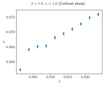
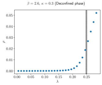
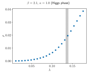
Figure 11: The spectral density at $\beta=1.9$ and $\kappa=1.0$ in the confined phase (top panel; here $N_{s}=20$), at $\beta=2.6$ and $\kappa=0.3$ in the deconfined phase (center panel; here $N_{s}=32$), and at $\beta=2.1$ and $\kappa=1.0$ in the Higgs phase (bottom panel; here $N_{s}=32$). In all plots $N_{t}=4$.

We now discuss eigenvalue observables, starting from the spectral density, Eq. (17), shown in Fig. 11. In the confined phase (top panel) the spectral density is practically constant in the lowest bins (except for the very lowest, which is depleted due to the smallness of the lattice volume), and grows as one moves towards the bulk of the spectrum. If we were in the chiral limit of massless fermions, a nonzero spectral density near the origin would indicate the spontaneous breaking of chiral symmetry [11]. Being in the opposite limit of infinitely massive fermions, we can speak of spontaneous chiral symmetry breaking only in a loose sense. In the deconfined and in the Higgs phase (bottom panels) we see instead that the spectral density is close to zero for near-zero modes, corresponding (again, loosely speaking) to the restoration of chiral symmetry. As we increase $\lambda$ the spectral density increases, and does so faster as one approaches the mobility edge. However, no sign of critical behavior is visible along the spectrum.

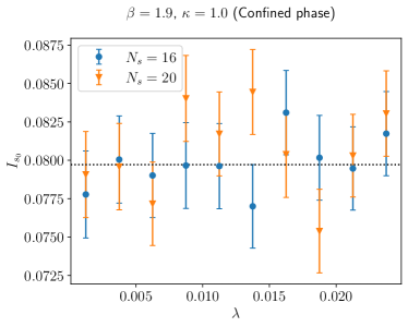
Figure 12: The integrated unfolded level spacing distribution $I_{s_{0}}$, Eq. (19), at $\beta=1.9$ and $\kappa=1.0$ in the confined phase. Here $N_{t}=4$. The horizontal dotted line shows the value of $I_{s_{0}}$ expected for RMT statistics.

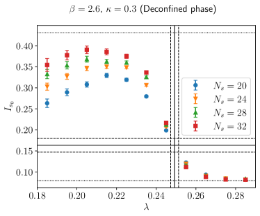
Figure 13: The integrated unfolded level spacing distribution $I_{s_{0}}$, Eq. (19), at $\beta=2.6$ and $\kappa=0.3$ in the deconfined phase. Here $N_{t}=4$. The upper and lower horizontal dotted lines show the value of $I_{s_{0}}$ expected for Poisson statistics and for RMT statistics, respectively. The vertical solid and dashed lines indicate the position and the error band of the mobility edge. The horizontal solid and dashed lines correspond to the estimate for the critical value $I_{s_{0},c}$ of $I_{s_{0}}$ at the mobility edge and its error band.

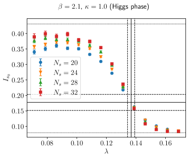
Figure 14: As in Fig. 13, but at $\beta=2.1$ and $\kappa=1.0$ in the Higgs phase. Here $N_{t}=4$.

We now move on to discuss the spectral statistic $I_{s_{0}}$, Eq. (19), for the low modes in the three different phases of the system. To estimate this quantity numerically we unfolded the spectrum, averaging then $I_{s_{0}}$ in small spectral bins and over gauge configurations. More precisely, we defined the unfolded spacings using Eq. (15), using for $\langle\lambda_{l+1}-\lambda_{l}\rangle_{\lambda}$ the average level spacing found in a given spectral bin, including all pairs of eigenvalues for which the smaller one fell in the bin.

In Fig. 12 we show $I_{s_{0}}$ in the confined phase. As expected, $I_{s_{0}}$ is compatible with the value predicted by RMT in the whole available spectral range for both volumes, further confirming that these modes are delocalized. In Figs. 13 and 14 we show the value of $I_{s_{0}}$ in the deconfined and in the Higgs phase. For modes near the origin $I_{s_{0}}$ approaches the value expected for Poisson statistics as we increase the volume, signaling that these are localized modes. For higher modes the value of $I_{s_{0}}$ tends instead to the RMT prediction as the volume increases, showing that modes are delocalized in this spectral region. Between these two regimes, we can find the mobility edge $\lambda_{c}$ as the point where $I_{s_{0}}$ is scale-invariant and the curves cross each other.

To find $\lambda_{c}$ and the critical value $I_{s_{0},c}$ of the spectral statistic we interpolated the numerical data with natural cubic splines, and determined the crossing point for the various pairs of system sizes using Cardano’s formula. The statistical error on each determination of $\lambda_{c}$ and $I_{s_{0},c}$ originating in the numerical uncertainty on $I_{s_{0}}$ in the various bins is estimated by obtaining the interpolating splines and their crossing point for a set of synthetic data, generating 100 data sets by drawing for each bin a number from a Gaussian distribution with mean equal to the average $I_{s_{0}}$ in the bin and variance equal to the square of the corresponding error. The systematic errors on $\lambda_{c}$ and $I_{s_{0},c}$ due to finite-size effects are estimated as the variance of the set of values for the crossing point and corresponding value of $I_{s_{0}}$ obtained from all the pairs of volumes. We finally estimated the mobility edge and the critical $I_{s_{0}}$ as those obtained from the crossing point of the biggest volume pair ($N_{s}=28,32$), as it should be the closest to the actual value in the infinite-volume limit, and the corresponding error by adding quadratically its statistical error with the finite-size systematic error discussed above. The total error is largely dominated by the finite-size contribution. We did this separately for the configurations in the deconfined and in the Higgs phase. The results for $\lambda_{c}$ and $I_{s_{0},c}$ are reported in Tab. 2, and shown in Figs. 13 and 14 as solid lines, with dashed lines marking the corresponding error bands. The two determinations of $I_{s_{0},c}$, obtained in the deconfined and in the Higgs phase, agree within errors. Despite the uncertainty on $I_{s_{0},c}$ being 10–15%, we could determine $\lambda_{c}$ with a 1–2% uncertainty thanks to the steepness of $I_{s_{0}}$ near the mobility edge.

$\beta$	$\kappa$	phase	$\lambda_{c}$	$I_{s_{0},c}$
$2.6$	$0.3$	deconfined	0.2493(20)	0.164(16)
$2.1$	$1.0$	Higgs	0.1367(24)	0.177(26)

Table 2: Mobility edge and critical value of $I_{s_{0}}$ estimated at two points of the phase diagram, one in the deconfined and one in the Higgs phase.

IV.3 $\beta$ and $\kappa$ dependence of the mobility edge

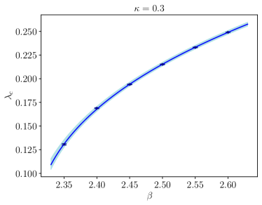
Figure 15: The dependence of the mobility edge on $\beta$ in the deconfined phase on the line at constant $\kappa=0.3$. The solid line is a power-law fit, Eq. (35), to the numerical data; the band corresponds to the finite-size systematic uncertainty discussed in the text. The point where the mobility edge vanishes is estimated at $\beta_{\mathrm{loc}}=2.2997(57)$, in the crossover region between the confined and deconfined phases, see Fig. 2 (bottom).

Having obtained estimates of $I_{s_{0},c}$ we can now use them to efficiently determine $\lambda_{c}$ throughout the phase diagram using a single lattice volume at each point, and looking for the point in the spectrum where $I_{s_{0}}$ takes the value $I_{s_{0},c}$. We use again natural cubic splines to interpolate the numerical data, using the more precise determination of $I_{s_{0},c}$ obtained in the deconfined phase and generating synthetic data as discussed above to estimate the statistical error. To estimate the magnitude of finite size effects, we determined also the crossing points $\lambda_{c,\pm}$ of $I_{s_{0}}$ with $I_{s_{0},c}\pm\delta I_{s_{0},c}$, with $\delta I_{s_{0},c}$ the uncertainty on $I_{s_{0},c}$. This is meant to determine just how much the crossing point of $I_{s_{0}}$ may change with the volume, as the error band on $I_{s_{0},c}$ is determined by the fluctuations of the crossing point of the various pairs of volumes used to find the mobility edge and the critical statistics in section IV.2, and has nothing to do with the fact that $I_{s_{0},c}$ is not known exactly. As explained in section II.2, one could in fact use any value intermediate between the RMT and the Poisson expectations to give an estimate of the mobility edge in a finite volume, and this would converge to the correct value in the thermodynamic limit.

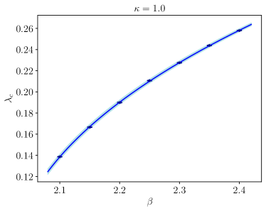
Figure 16: The dependence of the mobility edge on $\beta$ in the Higgs phase on the line at constant $\kappa=1.0$. The solid line is a power-law fit, Eq. (35), to the numerical data; the band corresponds to the finite-size systematic uncertainty discussed in the text. The point where the mobility edge vanishes is estimated at $\beta_{\mathrm{loc}}=2.0101(28)$, in the crossover region between the confined and Higgs phases, see Fig. 2 (center).

	deconfined	Higgs
$\beta_{\mathrm{loc}}$	2.2997(22)	2.0101(25)
$A$	0.3836(17)	0.3851(14)
$B$	0.3592(54)	0.4344(59)
$\chi^{2}/\mathrm{dof}$	1.48	1.64

Table 3: Parameters of a best fit of the $\beta$ dependence of the mobility edge in the deconfined ($\kappa=0.3$) and Higgs ($\kappa=1.0$) phases, with the fitting function in Eq. (35). Only statistical errors are reported.

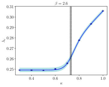
Figure 17: The dependence of the mobility edge on $\kappa$ on the line at constant $\beta=2.6$ in the deconfined and Higgs phases. The solid line is a fit to the data with Eq. (36); the band corresponds to the finite-size systematic uncertainty discussed in the text. A change of behavior is found at $\kappa_{\mathrm{loc}}=0.7303(59)$ in the crossover region between the two phases, see Fig. 2 (top), marked here by a vertical solid line, with dashed lines giving the corresponding error band.

We can then study how $\lambda_{c}$ depends on $\kappa$ and $\beta$. In Fig. 15 we show how $\lambda_{c}$ changes in the deconfined phase as one decreases $\beta$ towards the confined phase at fixed $\kappa$. We expect that the mobility edge disappears as we enter the confined phase and the Polyakov loop loses its strong ordering. To estimate the value $\beta_{\mathrm{loc}}(\kappa)$ of $\beta$ where this happens we fitted our results with a power-law function,

$$\lambda_{c}(\beta)=A\cdot(\beta-\beta_{\mathrm{loc}})^{B}\,,$$ (35)

using the MINUIT library [58] to minimize the $\chi^{2}$, computed using only the statistical errors on $\lambda_{c}$. We then repeated the fit using $\lambda_{c\pm}(\beta)$ to find the corresponding $\beta_{\mathrm{loc}\pm}$ where they extrapolate to zero, and used these to estimate the systematic uncertainty due to finite-size effects as $\frac{1}{2}|\beta_{\mathrm{loc}+}-\beta_{\mathrm{loc}-}|$. We obtained for the critical value $\beta_{\mathrm{loc}}(0.3)=2.2997(22)_{\mathrm{stat}}(53)_{\mathrm{syst}}=2.2997(57)$, where the total error is the sum in quadrature of the statistical error from the fit and of the systematic error. The other fit parameters and the $\chi^{2}$ per degree of freedom, $\chi^{2}/\mathrm{dof}=\chi^{2}/(n_{\mathrm{data}}-n_{\mathrm{parameters}})$, are reported in Tab. 3. The critical point is shown also in Fig. 2 (bottom), where we see that the vanishing of the mobility edge matches well with the crossover between the phases.

In Fig. 16 we show how $\lambda_{c}$ changes in the Higgs phase as one decreases $\beta$ towards the confined phase at fixed $\kappa$. Again, we expect the mobility edge to disappear at the crossover. For the critical $\beta_{\mathrm{loc}}(\kappa)$ we find $\beta_{\mathrm{loc}}(1.0)=2.0101(25)_{\mathrm{stat}}(13)_{\mathrm{syst}}=2.0101(28)$, again from a fit with a power law, Eq. (35), using statistical errors only (see Tab. 3 for the other fit parameters), and estimating systematic effects by fitting $\lambda_{c\pm}$, as discussed above. This is shown also in Fig. 2 (center), where one sees that the vanishing of $\lambda_{c}$ takes place again in the crossover region.

$\kappa_{\mathrm{loc}}$	0.7303(56)
$a$	0.24915(13)
$b$	0.1185(53)
$c$	0.1874(52)
$d$	26.4(2.0)
$\chi^{2}/\mathrm{dof}$	2.05

Table 4: Parameters of a best fit of the $\kappa$ dependence of the mobility edge in the deconfined and Higgs phases at $\beta=2.6$, with the fitting function in Eq. (36). Only statistical errors are reported.

The third case we examined is the transition from the Higgs phase to the deconfined phase as we decrease $\kappa$ at fixed $\beta$. This is shown in Fig. 17. One can see that at first $\lambda_{c}$ decreases quickly with $\kappa$, but below a critical value $\kappa_{\mathrm{loc}}(\beta)$ it becomes practically constant. The critical value is defined here as the point where the behavior changes from approximately constant to approximately linear, as obtained by fitting with the following function,

$$\lambda_{c}(\kappa) =a\cdot\left(1-\sigma\left(d\cdot(\kappa-\kappa_{\mathrm{loc}})\right)\right)$$ (36)

$$\phantom{=}+\left(b\kappa+c\right)\sigma(d\cdot(\kappa-\kappa_{\mathrm{loc}}))\,,$$

where $\sigma(x)={1}/{(1+e^{-x})}$ is the sigmoid function. Following the same procedure discussed above to estimate errors, we found $\kappa_{\mathrm{loc}}(2.6)=0.7303(57)_{\mathrm{stat}}(17)_{\mathrm{syst}}=0.7303(59)$ for the critical point (see Tab. 4 for the other fit parameters). As shown in Fig. 2 (top), also in this case the critical value matches well with the position of the crossover. Notice that here the critical point is not as sharply defined as in the previous two cases, as it simply corresponds to a change in the $\kappa$ dependence of the mobility edge, rather than its very appearance. However, it is possible that the change in the behavior of $\lambda_{c}(\kappa)$ becomes singular in the infinite-volume limit, e.g., due to a discontinuity in its derivative. If so, one would find a sharply defined critical point for the geometric transition also in this case. At the present stage this is only speculation, and a more careful determination of the mobility edge is needed to test this possibility, either by a proper finite-size scaling analysis, or by checking the volume dependence of the crossing point of $I_{s_{0}}$ with $I_{s_{0},c}$.

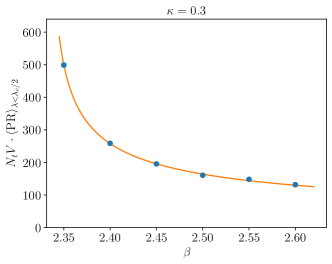
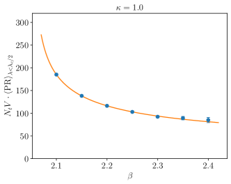
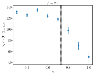
Figure 18: Mode size averaged up to $\lambda_{c}/2$, Eq. 37, at $\kappa=0.3$ in the deconfined phase (top panel) and at $\kappa=1.0$ in the Higgs phase (center panel), as a function of $\beta$, and at $\beta=2.6$ across the transition from the deconfined to the Higgs phase (bottom panel), as a function of $\kappa$. In all plots $N_{s}=20$ and $N_{t}=4$. The solid line in the top and center panels is a fit with a power-law function. The vertical and dashed lines in the bottom panel mark the critical value $\kappa_{\mathrm{loc}}$ and the corresponding error band [see after Eq. (36)].

	deconfined	Higgs
$\beta_{\mathrm{loc}}$	$2.3318(15)$	$2.0499(92)$
$a$	$67.2(2.1)$	$52.0(2.9)$
$b$	$0.501(17)$	$0.424(43)$
$\chi^{2}/\mathrm{dof}$	1.96	0.34

Table 5: Parameters of a best fit of the $\beta$ dependence of the average size of the lowest modes, $\langle N_{t}V\cdot\mathrm{PR}\rangle_{\lambda<\frac{\lambda_{c}}{2}}$, Eq. (37), with the fitting function in Eq. (38).

It is interesting to compare the estimates of $\beta_{\mathrm{loc}}$ and $\kappa_{\mathrm{loc}}$ obtained from eigenvalue observables to similar estimates obtained from eigenvector observables. In particular, if $\lambda_{c}$ vanishes continuously at $\beta_{\mathrm{loc}}$, then in the thermodynamic limit the localization length of the low modes should correspondingly diverge. We have then looked at the size of the low modes averaged over the lowest half of the localized spectral region,

$$N_{t}V\cdot\langle\mathrm{PR}\rangle_{\lambda<\frac{\lambda_{c}}{2}} =\frac{1}{\mathcal{N}({\textstyle\frac{\lambda_{c}}{2}})}\int_{0}^{\frac{\lambda_{c}}{2}}d\lambda\,\rho(\lambda)\,N_{t}V\cdot\mathrm{PR}(\lambda,N_{s})\,,$$ (37)

$$\mathcal{N}(\lambda_{0}) =\int_{0}^{\lambda_{0}}d\lambda\,\rho(\lambda)\,.$$

In Fig. 18 we show this quantity as a function of $\beta$ for constant $\kappa=0.3$ in the deconfined phase (top panel) and $\kappa=1.0$ in the Higgs phase (center panel). This quantity does indeed grow large as one approaches the confined phase. Fits with a power-law function,

$$N_{t}V\cdot\langle\mathrm{PR}\rangle_{\lambda<\frac{\lambda_{c}}{2}}=a\cdot(\beta-\beta_{\mathrm{loc}})^{-b}\,,$$ (38)

yield $\beta_{\mathrm{loc}}=2.3318(15)$ in the deconfined phase, and $\beta_{\mathrm{loc}}=2.0499(92)$ in the Higgs phase, both in the crossover region, and in reasonable agreement with the determinations based on the extrapolation of the mobility edge. Here one should take into account that the functional form Eq. (38) is not fully justified, as the mode size cannot diverge in a finite volume, and there is no reason to assume that the mode size goes to zero at large $\beta$. Nonetheless, one obtains decent fits (see the resulting fit parameters and $\chi^{2}$ in Tab. 5); adding a costant term makes them worse. On top of this, the error estimates do not include any uncertainty due to finite-size effects, which are large near $\beta_{\mathrm{loc}}$. For completeness, in the bottom panel of Fig. 18 we show $N_{t}V\cdot\langle\mathrm{PR}\rangle_{\lambda<\frac{\lambda_{c}}{2}}$ as a function of $\kappa$ at constant $\beta=2.6$ across the two phases. Here the data indicate a finite mode size at all $\kappa$, with a change from a constant to a steadily decreasing trend taking place at the crossover between the deconfined and the Higgs phase, showing that localized modes shrink rapidly as one moves deeper in the Higgs phase and the Polyakov-loop expectation value increases (see Fig. 1).

IV.4 Correlation with bosonic observables and sea/island mechanism

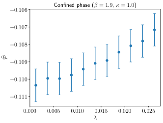
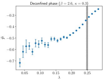
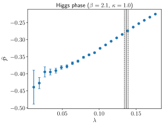
Figure 19: Polyakov loop weighted by Dirac modes, centered to its average and rescaled by the square root of its susceptibility, Eq. (21), at $\beta=1.9$ and $\kappa=1.0$ in the confined phase (top panel; here $N_{s}=20$), at $\beta=2.6$ and $\kappa=0.3$ in the deconfined phase (center panel; here $N_{s}=32$), and at $\beta=2.1$ and $\kappa=1.0$ in the Higgs phase (bottom panel; here $N_{s}=32$). In all plots $N_{t}=4$. In the center and bottom panels the solid line shows the value of the mobility edge, and the dashed lines indicate the corresponding error band.

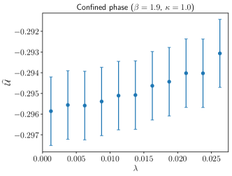
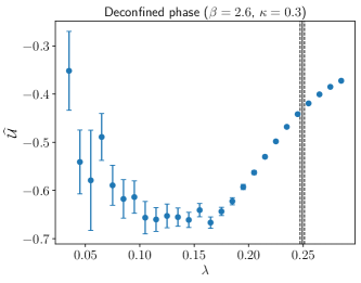
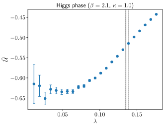
Figure 20: Plaquette weighted by Dirac modes, centered to its average and rescaled by the square root of its susceptibility, Eq. (21), at $\beta=1.9$ and $\kappa=1.0$ in the confined phase (top panel; here $N_{s}=20$), at $\beta=2.6$ and $\kappa=0.3$ in the deconfined phase (center panel; here $N_{s}=32$), and at $\beta=2.1$ and $\kappa=1.0$ in the Higgs phase (bottom panel; here $N_{s}=32$). In all plots $N_{t}=4$. In the center and bottom panels the solid line shows the value of the mobility edge, and the dashed lines indicate the corresponding error band.

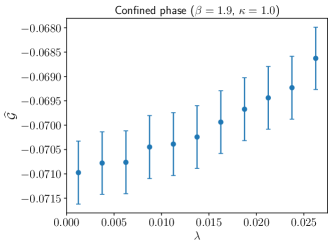
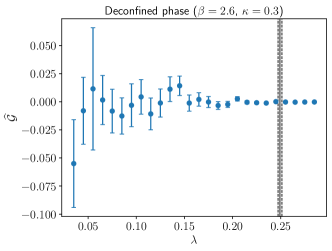
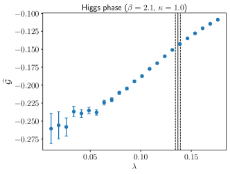
Figure 21: Gauge-Higgs coupling term weighted by Dirac modes, centered to its average and rescaled by the square root of its susceptibility, Eq. (21), at $\beta=1.9$ and $\kappa=1.0$ in the confined phase (top panel; here $N_{s}=20$), at $\beta=2.6$ and $\kappa=0.3$ in the deconfined phase (center panel; here $N_{s}=32$), and at $\beta=2.1$ and $\kappa=1.0$ in the Higgs phase (bottom panel; here $N_{s}=32$). In all plots $N_{t}=4$. In the center and bottom panels the solid line shows the value of the mobility edge, and the dashed lines indicate the corresponding error band.

We now proceed to discuss our results on the correlation of staggered eigenmodes with the gauge and Higgs fields. To this end, the most informative quantities are the centered and normalized observables $\widehat{\mathcal{U}}$, $\widehat{\mathcal{P}}$ and $\widehat{\mathcal{G}}$, defined in Eq. (21), that take into account the width of the distribution of the relevant bosonic observables. Our results for these quantities are shown in Figs. 19–21. The statistical error on the numerical estimate of these quantities is obtained by first determining the jackknife error on $\mathcal{U}$, $\mathcal{P}$ and $\mathcal{G}$, and correspondingly on $\langle U\rangle$, $\langle P\rangle$, $\langle G\rangle$ and on $(\delta U)^{2}$, $(\delta P)^{2}$, $(\delta G)^{2}$, followed by linear error propagation. Correlations with Polyakov-loop and plaquette fluctuations are always negative, showing that low modes prefer locations where these quantities fluctuate to values below their average. Correlations with gauge-Higgs coupling term fluctuations are again negative in the confined and in the Higgs phase, while they are essentially compatible with zero in the deconfined phase.

The correlation of low modes with Polyakov-loop fluctuations is shown in Fig. 19. In the confined phase this is small but significant, and decreasing very little in magnitude as one goes up in the spectral region that we explored. The strength of this correlation is considerably larger in the Higgs phase, and even larger in the deconfined phase. Since Polyakov-loop fluctuations are typically localized in these phases, this increased correlation is possible only if the low modes tend to localize on the corresponding locations. In both the deconfined and the Higgs phase one sees also a more rapid decrease in the magnitude of the correlation as one moves up in the spectrum. This, however, remains stronger than for the lowest modes in the confined phase also above the mobility edge.

The correlation of low modes with plaquette fluctuations is shown in Fig. 20. Also in this case a significant correlation is found in all three phases, generally stronger (and comparable in size) in the deconfined and Higgs phases than in the confined phase. Compared to the correlation with Polyakov-loop fluctuations, one finds a similar magnitude in the deconfined phase, and a larger magnitude in the Higgs phase. Since also plaquette fluctuations are typically localized, this means that they are at least as relevant as Polyakov-loop fluctuations for the localization of low modes. A clear upturn is visible for the lowest modes in the deconfined phase and, to a much smaller extent, also in the Higgs phase. We do not have an explanation for this. Even though the density of near-zero modes is very small in both cases, leading to large fluctuations, this upturn might be significant, as the mode size displays a similar behavior (see Figs. 8 and 9), with an increase in size for the lowest modes. (The downturn seen in $I_{s_{0}}$, Figs. 13 and 14, may also be related, but could also be a finite-size artifact caused by the low and rapidly changing density of modes, that makes our unfolding procedure not fully reliable in that spectral region.) The same upturn in the mode size is observed also in QCD [4], where it can be explained by the topological origin of the near-zero modes [59, 60]. Such modes are in fact expected to originate in the mixing of the localized zero modes associated with topological lumps in the gauge configuration at finite temperature, so extending over more than one such lump. While they fail to become delocalized due to the low density of lumps at high temperature, they nonetheless should display a larger size than localized modes not of topological origin. This picture is consistent with the strong correlation between localized near-zero modes and the local topology of the gauge configuration, demonstrated in Ref. [7], and with the lumpy nature of near-zero Dirac modes in high-temperature QCD, demonstrated in Ref. [61]. A similar mechanism could explain the larger size of the lowest modes observed here. Interestingly, no upturn in the size of the lowest modes is observed in 2+1 dimensional pure $\mathrm{SU}(3)$ gauge theory [24] or in 2+1 dimensional discrete gauge theories [27, 16], where the topology of gauge field configurations is trivial.

Finally, the correlation of low modes with fluctuations of the gauge-Higgs coupling term is shown in Fig. 21. A very mild correlation is visible in the confined phase, no significant correlation is found in the deconfined phase, and a clear but small correlation is found in the Higgs phase, weaker than the correlation with Polyakov-loop and plaquette fluctuations. This leads us to conclude that these fluctuations are much less relevant to low-mode localization.

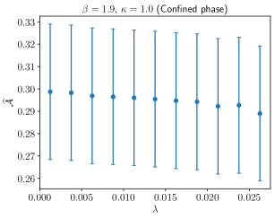
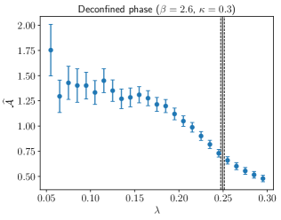
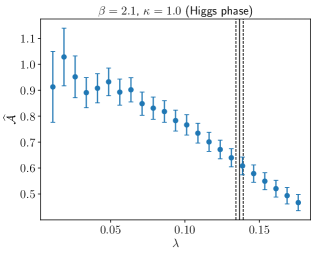
Figure 22: The quantity $\widehat{\mathcal{A}}$, Eq. (32), measuring the correlation of staggered modes with fluctuations of $A(\vec{x})$, Eq. (31), at $\beta=1.9$ and $\kappa=1.0$ in the confined phase (top panel; here $N_{s}=16$), at $\beta=2.6$ and $\kappa=0.3$ in the deconfined phase (center panel; here $N_{s}=20$), and at $\beta=2.1$ and $\kappa=1.0$ in the Higgs phase (bottom panel; here $N_{s}=20$). In all plots $N_{t}=4$. In the center and bottom panels the solid line shows the value of the mobility edge, and the dashed lines indicate the corresponding error band.

We then studied the sea/island mechanism directly by looking at the correlation of the staggered eigenmodes with the local fluctuations of the hopping term in the Dirac-Anderson Hamiltonian, measured by the quantity $A$ of Eq. (30). To this end we analyzed 450 configurations with $N_{s}=16$ in the confined phase, and 1400 configurations with $N_{s}=20$ in the deconfined and Higgs phases, with $N_{t}=4$ in both cases. The average value of $A$ drops substantially as one moves from the confined to the deconfined or to the Higgs phase: for the given lattice sizes (but this quantity is not expected to show a strong volume dependence), $\langle A\rangle=0.2761(11)$ at $\beta=1.9,\kappa=1.0$ in the confined phase; $\langle A\rangle=0.15828(64)$ at $\beta=2.6,\kappa=0.3$ in the deconfined phase; and $\langle A\rangle=0.20518(86)$ at $\beta=2.1,\kappa=1.0$ in the Higgs phase. This is expected to happen, as a consequence of the ordering of the Polyakov loop and the resulting strong correlation in the temporal direction [16].

The centered and normalized quantity $\widehat{\mathcal{A}}$ defined in Eq. (32) is shown in Fig. 22. This quantity correlates positively with the spatial density of low modes in all phases, in agreement with the refined sea/islands picture of Ref. [16]. In the confined phase the magnitude of the correlation with fluctuations in this quantity is comparable with the correlation with plaquette fluctuations, and independent of the position in the spectrum in the available region, within errors. In the Higgs and, especially, in the deconfined phase this correlation is much stronger than those with Polyakov-loop and with plaquette fluctuations. Although it remains strong also at the beginning of the bulk region, it reduces by about a third when going from the lowest modes to the first delocalized modes right above the mobility edge. Since fluctuations of $A(\vec{x})$ are typically localized in the deconfined and Higgs phases, this result strongly suggests that they are the ones mainly responsible for trapping the eigenmodes in space.

V Conclusions

A strong connection has emerged in recent years between the deconfinement phase transition in gauge theories with or without fermionic matter, and the change in the localization properties of low Dirac modes [3, 4, 5, 6, 7, 8, 9, 10, 18, 19, 20, 21, 22, 12, 13, 14, 15, 23, 28, 24, 25, 26, 29, 27, 16]. In this paper we extended this line of research by studying the lattice $\mathrm{SU}(2)$-Higgs model with a Higgs field of fixed length [36, 37, 38, 39, 40, 41, 42] at finite temperature, probed with external static fermions. The extension is twofold. On the one hand, this model has dynamical scalar rather than fermionic matter: while one still expects localized modes in the deconfined phase of the model, as the nature of the dynamical matter does not affect the general argument for localization [12, 13, 14, 15, 10, 16], it is nonetheless useful to verify this explicitly. On the other hand, and more interestingly, the two-parameter phase diagram of this model displays a third phase besides the confined and deconfined phases, i.e., the Higgs phase: one can then check whether or not modes are localized in this phase, and if so whether the onset of localization is related in any way to the thermodynamic transition.

A survey of the phase diagram shows the expected tripartition into a confined, a deconfined, and a Higgs phase, separated by analytic crossovers [42]. The deconfined and the Higgs phases are distinguished from the confined phase by a much larger expectation value of the Polyakov loop, and from each other by the expectation value of the Higgs-coupling term, much larger in the Higgs phase than in the deconfined and in the confined phases. Since the Polyakov loop is strongly ordered, one expects localization of low Dirac modes to take place in both phases [12, 13, 14, 15, 10, 16].

By means of numerical simulations, we have demonstrated that localized modes are indeed present both in the deconfined and in the Higgs phase. In both cases, the mobility edge separating localized and delocalized modes in the spectrum decreases as one moves towards the confined phase, and disappears as one reaches the crossover region. At the transition between the deconfined and the Higgs phase, instead, the dependence of the mobility edge on the gauge-Higgs coupling constant changes from almost constant to steadily increasing. These findings provide further support to the universal nature of the sea/islands picture of localization [12, 13, 14, 15, 10, 16] in a previously unexplored setup in the presence of dynamical scalar matter.

We have then studied the sea/islands mechanism in more detail, measuring the correlation between localized modes and fluctuations of the gauge and Higgs fields. We found a strong correlation with Polyakov-loop and plaquette fluctuations both in the deconfined and in the Higgs phase, and a mild but significant correlation with fluctuations of the gauge-Higgs coupling term only in the Higgs phase. Moreover, we found in both phases a very strong correlation (stronger than that with Polyakov-loop or plaquette fluctuations) with the type of gauge-field fluctuations identified in Ref. [16] as the most relevant to localization. This provides further evidence for the validity of the refined sea/islands picture proposed in Ref. [16].

A possible extension of this work would be a study of the low $\beta$, large $\kappa$ corner of the phase diagram, where the crossover becomes very weak, in order to check if the line of “geometric” transitions where the mobility edge in the Dirac spectrum vanishes extends all the way to $\beta=0$, or if instead it has an endpoint. This is interesting also in connection with the “spin glass” approach of Ref. [44]: since in that region of parameter space this predicts a transition line clearly distinct from the one found with more traditional approaches based on gauge fixing, one would like to compare this line with the one defined by the vanishing of the mobility edge (if the latter exists). A different direction would be the study of the localization properties of the eigenmodes of the covariant Laplacian, extending to finite temperature and dynamical scalar matter the work of Refs. [62, 63].

References

- Aoki et al. [2006] Y. Aoki, G. Endrődi, Z. Fodor, S. D. Katz, and K. K. Szabó, Nature 443, 675 (2006), arXiv:hep-lat/0611014 .
- Bazavov et al. [2012] A. Bazavov et al., Phys. Rev. D 85, 054503 (2012), arXiv:1111.1710 [hep-lat] .
- García-García and Osborn [2007] A. M. García-García and J. C. Osborn, Phys. Rev. D 75, 034503 (2007), arXiv:hep-lat/0611019 [hep-lat] .
- Kovács and Pittler [2012] T. G. Kovács and F. Pittler, Phys. Rev. D 86, 114515 (2012), arXiv:1208.3475 [hep-lat] .
- Giordano et al. [2014] M. Giordano, T. G. Kovács, and F. Pittler, Phys. Rev. Lett. 112, 102002 (2014), arXiv:1312.1179 [hep-lat] .
- Ujfalusi et al. [2015] L. Ujfalusi, M. Giordano, F. Pittler, T. G. Kovács, and I. Varga, Phys. Rev. D 92, 094513 (2015), arXiv:1507.02162 [cond-mat.dis-nn] .
- Cossu and Hashimoto [2016] G. Cossu and S. Hashimoto, J. High Energy Phys. 06, 056 (2016), arXiv:1604.00768 [hep-lat] .
- Holicki et al. [2018] L. Holicki, E.-M. Ilgenfritz, and L. von Smekal, PoS LATTICE2018, 180 (2018), arXiv:1810.01130 [hep-lat] .
- Kehr et al. [2023] R. Kehr, D. Smith, and L. von Smekal, arXiv:2304.13617 [hep-lat] (2023).
- Giordano and Kovács [2021] M. Giordano and T. G. Kovács, Universe 7, 194 (2021), arXiv:2104.14388 [hep-lat] .
- Banks and Casher [1980] T. Banks and A. Casher, Nucl. Phys. B 169, 103 (1980).
- Bruckmann et al. [2011] F. Bruckmann, T. G. Kovács, and S. Schierenberg, Phys. Rev. D 84, 034505 (2011), arXiv:1105.5336 [hep-lat] .
- Giordano et al. [2015] M. Giordano, T. G. Kovács, and F. Pittler, J. High Energy Phys. 04, 112 (2015), arXiv:1502.02532 [hep-lat] .
- Giordano et al. [2016] M. Giordano, T. G. Kovács, and F. Pittler, J. High Energy Phys. 06, 007 (2016), arXiv:1603.09548 [hep-lat] .
- Giordano et al. [2017a] M. Giordano, T. G. Kovács, and F. Pittler, Phys. Rev. D 95, 074503 (2017a), arXiv:1612.05059 [hep-lat] .
- Baranka and Giordano [2022] G. Baranka and M. Giordano, Phys. Rev. D 106, 094508 (2022), arXiv:2210.00840 [hep-lat] .
- Note [1] A notable exception is when the (untraced) Polyakov loops order along minus the identity, in which case low modes remain delocalized also in the deconfined phase [27].
- Göckeler et al. [2001] M. Göckeler, P. E. L. Rakow, A. Schäfer, W. Söldner, and T. Wettig, Phys. Rev. Lett. 87, 042001 (2001), arXiv:hep-lat/0103031 [hep-lat] .
- Gattringer et al. [2001] C. Gattringer, M. Göckeler, P. E. L. Rakow, S. Schaefer, and A. Schäfer, Nucl. Phys. B 618, 205 (2001), arXiv:hep-lat/0105023 [hep-lat] .
- Gavai et al. [2008] R. V. Gavai, S. Gupta, and R. Lacaze, Phys. Rev. D 77, 114506 (2008), arXiv:0803.0182 [hep-lat] .
- Kovács [2010] T. G. Kovács, Phys. Rev. Lett. 104, 031601 (2010), arXiv:0906.5373 [hep-lat] .
- Kovács and Pittler [2010] T. G. Kovács and F. Pittler, Phys. Rev. Lett. 105, 192001 (2010), arXiv:1006.1205 [hep-lat] .
- Kovács and Vig [2018] T. G. Kovács and R. Á. Vig, Phys. Rev. D 97, 014502 (2018), arXiv:1706.03562 [hep-lat] .
- Giordano [2019] M. Giordano, J. High Energy Phys. 05, 204 (2019), arXiv:1903.04983 [hep-lat] .
- Vig and Kovács [2020] R. Á. Vig and T. G. Kovács, Phys. Rev. D 101, 094511 (2020), arXiv:2001.06872 [hep-lat] .
- Bonati et al. [2021] C. Bonati, M. Cardinali, M. D’Elia, M. Giordano, and F. Mazziotti, Phys. Rev. D 103, 034506 (2021), arXiv:2012.13246 [hep-lat] .
- Baranka and Giordano [2021] G. Baranka and M. Giordano, Phys. Rev. D 104, 054513 (2021), arXiv:2104.03779 [hep-lat] .
- Giordano et al. [2017b] M. Giordano, S. D. Katz, T. G. Kovács, and F. Pittler, J. High Energy Phys. 02, 055 (2017b), arXiv:1611.03284 [hep-lat] .
- Cardinali et al. [2022] M. Cardinali, M. D’Elia, F. Garosi, and M. Giordano, Phys. Rev. D 105, 014506 (2022), arXiv:2110.10029 [hep-lat] .
- Ghanbarpour and von Smekal [2022] M. Ghanbarpour and L. von Smekal, Phys. Rev. D 106, 054513 (2022), arXiv:2206.11697 [hep-lat] .
- Myers and Ogilvie [2008] J. C. Myers and M. C. Ogilvie, Phys. Rev. D 77, 125030 (2008), arXiv:0707.1869 [hep-lat] .
- Ünsal and Yaffe [2008] M. Ünsal and L. G. Yaffe, Phys. Rev. D 78, 065035 (2008), arXiv:0803.0344 [hep-th] .
- Bonati et al. [2018] C. Bonati, M. Cardinali, and M. D’Elia, Phys. Rev. D 98, 054508 (2018), arXiv:1807.06558 [hep-lat] .
- Bonati et al. [2020] C. Bonati, M. Cardinali, M. D’Elia, and F. Mazziotti, Phys. Rev. D 101, 034508 (2020), arXiv:1912.02662 [hep-lat] .
- Athenodorou et al. [2021] A. Athenodorou, M. Cardinali, and M. D’Elia, Phys. Rev. D 104, 074510 (2021), arXiv:2010.03618 [hep-lat] .
- Fradkin and Shenker [1979] E. H. Fradkin and S. H. Shenker, Phys. Rev. D 19, 3682 (1979).
- Lang et al. [1981] C. B. Lang, C. Rebbi, and M. Virasoro, Phys. Lett. B 104, 294 (1981).
- Montvay [1985] I. Montvay, Phys. Lett. B 150, 441 (1985).
- Montvay [1986] I. Montvay, Nucl. Phys. B 269, 170 (1986).
- Langguth and Montvay [1985] W. Langguth and I. Montvay, Phys. Lett. B 165, 135 (1985).
- Campos [1998] I. Campos, Nucl. Phys. B 514, 336 (1998), arXiv:hep-lat/9706020 .
- Bonati et al. [2010] C. Bonati, G. Cossu, M. D’Elia, and A. Di Giacomo, Nucl. Phys. B 828, 390 (2010), arXiv:0911.1721 [hep-lat] .
- Lautrup and Nauenberg [1980] B. E. Lautrup and M. Nauenberg, Phys. Rev. Lett. 45, 1755 (1980).
- Greensite and Matsuyama [2022] J. Greensite and K. Matsuyama, Symmetry 14, 177 (2022), arXiv:2112.06421 [hep-lat] .
- Mehta [2004] M. L. Mehta, Random matrices, 3rd ed., Pure and Applied Mathematics, Vol. 142 (Academic Press, 2004).
- Verbaarschot and Wettig [2000] J. J. M. Verbaarschot and T. Wettig, Ann. Rev. Nucl. Part. Sci. 50, 343 (2000), arXiv:hep-ph/0003017 [hep-ph] .
- Note [2] Since , eigenmodes in a degenerate pair have identical .
- Evers and Mirlin [2008] F. Evers and A. D. Mirlin, Rev. Mod. Phys. 80, 1355 (2008), arXiv:0707.4378 [cond-mat.mes-hall] .
- Al’tshuler and Shklovskiĭ [1986] B. L. Al’tshuler and B. I. Shklovskiĭ, Sov. Phys. JETP 64, 127 (1986).
- Shklovskiĭ et al. [1993] B. I. Shklovskiĭ, B. Shapiro, B. R. Sears, P. Lambrianides, and H. B. Shore, Phys. Rev. B 47, 11487 (1993).
- Note [3] In the definition of in Eq. (B.8) of Ref. [16] the factors and are incorrectly missing.
- Engels et al. [1990] J. Engels, J. Fingberg, and M. Weber, Nucl. Phys. B 332, 737 (1990).
- Engels et al. [1992] J. Engels, J. Fingberg, and D. E. Miller, Nucl. Phys. B 387, 501 (1992).
- Engels et al. [1993] J. Engels, J. Fingberg, and V. K. Mitrjushkin, Phys. Lett. B 298, 154 (1993).
- Engels et al. [1996] J. Engels, S. Mashkevich, T. Scheideler, and G. Zinovev, Phys. Lett. B 365, 219 (1996), arXiv:hep-lat/9509091 .
- Stathopoulos and McCombs [2010] A. Stathopoulos and J. R. McCombs, ACM Transactions on Mathematical Software 37, 21:1 (2010).
- Wu et al. [2017] L. Wu, E. Romero, and A. Stathopoulos, SIAM Journal on Scientific Computing 39, S248 (2017), arXiv:1607.01404 [cs.MS] .
- James and Roos [1975] F. James and M. Roos, Comput. Phys. Commun. 10, 343 (1975).
- Edwards et al. [2000] R. G. Edwards, U. M. Heller, J. E. Kiskis, and R. Narayanan, Phys. Rev. D 61, 074504 (2000), arXiv:hep-lat/9910041 .
- Vig and Kovács [2021] R. Á. Vig and T. G. Kovács, Phys. Rev. D 103, 114510 (2021), arXiv:2101.01498 [hep-lat] .
- Meng et al. [2023] X.-L. Meng, P. Sun, A. Alexandru, I. Horváth, K.-F. Liu, G. Wang, and Y.-B. Yang (QCD, CLQCD), arXiv:2305.09459 [hep-lat] (2023).
- Greensite et al. [2005] J. Greensite, Š. Olejník, M. Polikarpov, S. Syritsyn, and V. Zakharov, Phys. Rev. D 71, 114507 (2005), arXiv:hep-lat/0504008 [hep-lat] .
- Greensite et al. [2006] J. Greensite, A. V. Kovalenko, Š. Olejník, M. I. Polikarpov, S. N. Syritsyn, and V. I. Zakharov, Phys. Rev. D 74, 094507 (2006), arXiv:hep-lat/0606008 [hep-lat] .