Fallback rates in partial tidal disruptions of white dwarfs by intermediate mass black holes

Abstract

Fallback rate of debris after a partial tidal disruption event of a star with an intermediate mass black hole (IMBH) might provide important signatures of such black holes, compared to supermassive ones. Here using smoothed particle hydrodynamics methods, we provide a comprehensive numerical analysis of this phenomenon. We perform numerical simulations of single partial tidal disruptions of solar mass white dwarfs in parabolic orbits, with a non-spinning $10^{3}M_{\odot}$ IMBH for various values of the impact parameter, and determine the core mass fractions and fallback rates of debris into the IMBH. For supermassive black holes, in a full disruption processes, it is known that the late time fallback rate follows a power law $t^{-5/3}$, whereas for partial disruptions, such a rate has been recently conjectured to saturate to a steeper power law $t^{-9/4}$, independent of the mass of the remnant core. We show here that for IMBHs, partial disruptions significantly alter this conclusion. That is, the fallback rate at late times do not asymptote to a $t^{-9/4}$ power law, and this rate is also a strong function of the core mass. We derive a robust formula for the late time fallback rate as a function of the core mass fraction, that is independent of the white dwarf mass, as we verify numerically by varying the mass of the white dwarf.

1 Introduction

Intermediate mass black holes (IMBHs, see Greene et al. (2020) for a recent review) have been dubbed as the ‘missing link’ in the theory of black hole (BH) formation and evolution. These BHs have masses $\sim 10^{2}-10^{5}M_{\odot}$ and are believed to exist, for example, in dwarf galaxies and globular clusters, and are possible seeds of supermassive black holes (SMBHs), see e.g., Volonteri (2012). There are however only a handful of recent observational evidences for these (Kızıltan et al., 2017; Chilingarian et al., 2018; Takekawa et al., 2019; Abbott et al., 2020; Lin et al., 2020), in contrast to the many confirmed observations of SMBHs and stellar mass black holes. Physical properties of IMBHs are thus important and interesting to study further. An important phenomenon that can serve as a distinctive feature of IMBHs are tidal disruption events (TDEs), since electromagnetic emission arising out of these events have a strong dependence on the BH mass. Generically, TDEs from BHs produce a luminous flare, and several such events have been detected (Holoien et al., 2019). Light curves from TDEs have been shown to broadly conform to theoretical predictions (Brown et al., 2015), and hence, observations of TDEs from IMBHs might be a crucial signature of the latter. In this context, another well studied object in stellar astrophysics is the tidal disruption of white dwarf (WD). The sufficiently accurate equation of state of a WD makes it an attractive object to study in this scenario. Now, it is well known that WDs can only be tidally disrupted by IMBHs and are captured by SMBHs, see the book chapter by Maguire et. al. in Jonker et al. (2022). TDEs involving WDs and IMBHs can thus be an ideal laboratory to glean further insight into the distinction between IMBHs and SMBHs. With this motivation, the purpose of this paper is to perform a comprehensive analysis of partial TDEs involving WDs in the background of IMBHs.

Recall that a stellar object is tidally disrupted by a BH when its self gravity is overcome by the non-local gravitational effects of the BH. From a Newtonian perspective, a TDE occurs when the pericenter position $r_{p}$ of a spherical star of mass $M_{\star}$ and radius $R_{\star}$ comes within the tidal radius $r_{t}\sim R_{\star}(M_{\rm BH}/M_{\star})^{1/3}$, with $M_{\rm BH}$ being the mass of the BH, see Hills (1975) and related early works by Frank & Rees (1976), Lacy et al. (1982), Carter & Luminet (1982), Carter & Luminet (1983). This is obtained by simply equating the tidal force on the spherical stellar object to its self gravity, but is often used as an order of magnitude estimate in more realistic situations when a star can be considerably deformed before being disrupted. In the presence of a tidal force, a star can be fully disrupted wherein it breaks up completely and is reduced to a stream of debris (Kochanek, 1994; Guillochon et al., 2014), or the disruption can be partial, leading to a remnant core, along with the debris (Manukian et al., 2013; Gafton et al., 2015; Banerjee et al., 2023). Once full tidal disruption has taken place, roughly half of the debris is bound to the BH and in time returns to the pericenter and falls into the BH. The situation is modified in partial disruption processes, but in due course, for both full and partial disruptions, the in-falling material dissipates energy and results in accretion flow, and can cause a luminous event (Evans & Kochanek, 1989; Hayasaki et al., 2013, 2016; Bonnerot et al., 2016; Liptai et al., 2019; Clerici & Gomboc, 2020). Also, the process of partial tidal disruption can in principle occur multiple times (MacLeod et al., 2013), if initial conditions allow the remnant core to come back to a new pericenter position. TDEs have been extensively investigated over more than four decades now, and continue to be an active research area in stellar astrophysics. For a sampling of the more recent literature, see, e.g., Lodato et al. (2009), Guillochon & Ramirez-Ruiz (2013), Tejeda & Rosswog (2013), Coughlin & Nixon (2015). Other studies include the effect on TDEs due to the black hole’s mass and spin (Chen & Shen, 2018; Gafton & Rosswog, 2019; Ryu et al., 2020a; Wang et al., 2021), stellar structure (Golightly et al., 2019a; Law-Smith et al., 2019; Ryu et al., 2020b), stellar rotation (Golightly et al., 2019b; Kagaya et al., 2019; Sacchi & Lodato, 2019; Law-Smith et al., 2017) and stellar orbital parameters (Darbha et al., 2019; Miles et al., 2020; Park & Hayasaki, 2020; Cufari et al., 2022), to name a few. A comprehensive recent review of various features of TDEs can be found in Jonker et al. (2022). An updated catalog of candidate TDEs can be found at the Open TDE Catalog (2023).

Ubiquitous in the study of tidal disruptions – both full and partial – is the notion of the fallback rate of bound debris into the BH. This is an important quantity to study, since it influences several features of light curves from TDEs. The fallback of debris starts when the most bound debris returns to the BH, with the rate of fallback reaching a maximum (called the peak fallback rate), and then asymptotes to a power law behaviour with time, for late times. A fundamental quantity of interest in this context is this late-time power law scaling, i.e., the mass fallback rate of tidal debris ${\dot{M}}\sim t^{n}$. A considerable amount of literature exists on the topic till date, with the initial result by Rees (1988) that $n=-5/3$ (the work Rees (1988) quotes the exponent as $-5/2$ and this was subsequently corrected by Phinney (1989) to $-5/3$, see also Ulmer (1999)). The argument is simple and only depends on Kepler’s third law. Although the process of tidal disruptions is reasonably complicated and the forces on the debris are not strictly central even at late times due to the presence of gravity among the debris particles, it is still a good estimate at late times, as shown by Lodato et al. (2009). This is because at late times, the density of the remaining debris is small, and Keplerian dynamics is often a reasonable approximation. While this power law has been tested for full TDEs in a number of notable works, see, e.g., Evans & Kochanek (1989), Coughlin & Nixon (2015), Law-Smith et al. (2020), it was established more recently that partial disruptions might considerably alter the situation. The essential point here is that after a partial disruption process, the core exerts gravitational influence on the debris that is bound to the BH, a fact that is irrelevant in full TDEs where there is no core to begin with. Now, the late time fallback rate is considerably influenced by the core, since particles falling back into the BH at such times originate close to the core itself. Naively, this is associated with the Hill radius of the core – a distance up to which gravitational influence of the core is greater than that of the BH.

The first indication that the late time peak fallback rate might be steeper than the $t^{-5/3}$ power law was provided by Guillochon & Ramirez-Ruiz (2013) where it was observed that the exponent was, in some cases, close to $-2.2$ for TDEs by SMBHs. Following this, recently, Coughlin & Nixon (2019) provided an analytical treatment of the power law behaviour of the late time peak fallback rate from SMBHs. They found that for full TDEs from such BHs, ${\dot{M}}\sim t^{-5/3}$ in accordance with previous analytical results and simulations, but that for partial TDEs, ${\dot{M}}\sim t^{-9/4}$. The latter represents a significant departure from the full TDE case, and it was argued by Coughlin & Nixon (2019) that this power law is effectively independent of the core mass fraction. As pointed out by Ryu et al. (2020c), this analysis has a number of assumptions, one of the main ones being that the force on the debris by the core is radial in direction. Indeed, the dynamics of the debris even at late times is complicated especially in the presence of a remnant core. Taking the Hill radius as a rough estimate of the influence of the core, one finds (both analytically and numerically) that this radius increases with time, and hence the core should continue to influence the falling debris even at late times. This indicates that Keplerian dynamics would be strictly invalid even at such late times. The behaviour of the late time slope of the fallback rate should therefore be carefully checked with numerical simulations. This was indeed done by Miles et al. (2020), who found from simulations of a $1M_{\odot}$ polytropic star in the background of a non-rotating $10^{6}M_{\odot}$ BH that ${\dot{M}}\sim t^{-9/4}$ was reasonably accurate and that the exponent was effectively independent of the remnant core, as suggested by analytical results. However, immediately afterwards, Wang et al. (2021) performed a similar analysis of TDEs involving stellar mass black holes. They find that the late time fallback rate was significantly different from a $t^{-9/4}$ law.

In this paper, we ask the question if the same is true for the TDE of a $1M_{\odot}$ WD by an IMBH. The main motivation for this study is that, as mentioned in the beginning of this paper, there is currently not enough compelling observational evidence of IMBHs, and in such a situation, any further analysis that can shed light on the physical properties of IMBHs should be important and interesting. WDs that come close to such an IMBH will be tidally disrupted either fully or partially, and such TDEs can play a vital role in detecting these objects. Further, accurate equations of state for WDs are well established, and using these, one can effectively revisit the results of Coughlin & Nixon (2019) to see to what extent the late time slope of the fallback rate, originally derived for SMBHs are applicable to IMBHs. Indeed, as we show in the course of this paper, we find significant departures from the results of Coughlin & Nixon (2019). One of our main results is that for IMBHs, there is a strong dependence of the late time slope of the fallback rate on the remnant core mass, contrary to the SMBH case. Here, we consider single-encounter, full and partial disruptions of WDs in parabolic orbits. A recent work by Chen et al. (2023) considers multiple tidal interactions of a WD that is in-spiralling into an IMBH.

The purpose of the rest of the paper then is to carry out a comprehensive analysis of TDEs involving a solar mass WD and a $10^{3}M_{\odot}$ IMBH. For various values of the impact parameter. This is done using using 15 smoothed particle hydrodynamics simulations of such events by varying the impact parameter. We study (a) the core mass fraction, (b) the peak fallback rate, (c) the instantaneous power law index of the fallback rate and (d) the late time slope of the fallback rate as functions of the impact parameter. In addition, 7 more numerical simulations were performed to check the robustness of our results for WDs with different masses, while keeping the black hole mass fixed. In the next section 2, we describe the methodology, followed by the results of our numerical analysis in section 3. Section 4 concludes this paper with a summary of our main results.

2 Methodology

In this section, we present our numerical methodology for simulating the tidal disruption of WDs by an IMBH. For a detailed description of the numerical methods employed here, we refer the reader to Banerjee et al. (2023) and avoid repeating the details here for brevity. Our simulation of the fluid star uses the smoothed particle hydrodynamics (SPH) technique, which discretizes the fluid star into a set of particles, each possessing density, position, velocity, and other properties. To efficiently compute fluid properties and forces on each particle, we implement a binary tree with a tree opening angle parameter set at $\theta=0.5$. Standard SPH artificial viscosity parameters, $\alpha^{\rm{AV}}=1.0$ and $\beta^{\rm{AV}}=2.0$ (see Hayasaki et al. (2013)), are adopted, while the Balsara switch is used to reduce the viscosity in shear flows (see Balsara (1995)). The SPH fluid equations are integrated using the leapfrog integrator, ensuring the exact conservation of energy and angular momentum throughout the simulation. In modeling the external gravitational influence on each particle originating due to the Schwarzschild black hole, we adopt the same approach as detailed in Banerjee et al. (2023). In this work, we employ a global time step for the evolution of the system.

We perform two-stage numerical simulations to study tidal disruption events. Initially, we create a spherically symmetric WD in equilibrium. Once the WD is modeled, we induce tidal disruption by setting the WD in motion under the gravitational influence of the black hole. To attain the equilibrium structure of a carbon-oxygen WD using the SPH formalism, we follow the methodology described in Garain et al. (2023). Hydrostatic equilibrium within the WD is attained when the pressure resulting from degenerate electrons balances the self-gravitational forces causing its collapse. The pressure due to degenerate electrons and the density originating from carbon atoms within the WD are expressed as follows:

$$P=K_{P}\Bigl{[}x(1+x^{2})^{1/2}(2x^{2}/3-1)+\log_{e}\bigl{[}x+(1+x^{2})^{1/2}\bigr{]}\Bigr{]},~{}\rho=K_{\rho}x^{3}$$ (1)

where the constants are defined as $K_{P}=1.4218\times 10^{24}/(8\pi^{2})$ $\rm N~{}m^{-2}$, $K_{\rho}=1.9479\times 10^{9}$ $\rm kg~{}m^{-3}$, and $x$ represents the ‘relativity parameter’ (dimensionless Fermi momentum). Consequently, the pressure and density are related through the parameter $x$, which serves as the equation of state (EOS) for our study. In SPH, particles are initially distributed in a closed-packed sphere, which is then stretched to attain the density profile for the WD, which is obtained by employing the methodology outlined in Garain et al. (2023). Subsequently, this stretched SPH profile of the fluid star is evolved in isolation, without the presence of the black hole, in order to smoothen out the density fluctuations. The final relaxed profile of the fluid star is achieved once its density profile matches exactly with the WD density profile.

In our study, we consider an IMBH with a mass $M_{\rm BH}=10^{3}M_{\odot}$, modeled as a Schwarzschild black hole situated at the origin. We construct the relaxed WD, which has a mass $M_{\rm wd}=1.00\,M_{\odot}$ and a radius of $R_{\rm wd}=0.0082\,R_{\odot}$. The center of mass of this relaxed WD is then placed at a distance of $5r_{t}$ from the black hole, where $r_{t}$ is the tidal radius as mentioned earlier. We vary the impact parameter, denoted as $\beta=r_{t}/r_{p}$, ranging from $0.48$ to $1.00$, with each WD following a parabolic trajectory. Initially, the positions and velocities of all particles following the appropriate trajectories are calculated using the method explained in Banerjee et al. (2023).

In this work, one of our main goals will be to calculate the fallback rates while varying the impact parameter. When the WD approaches the black hole and has a relatively weak interaction at its closest point, some of the WD’s material is disrupted. The extent of this disruption increases when the encounter is deeper, meaning that the pericenter distance is closer. We note that we are not concerned here with the circularization and disk formation processes. Therefore, after the interaction, once the WD moves away from the black hole and reaches a significant distance, we expand the accretion radius to $3r_{t}\simeq 116r_{g}$, where $r_{g}=GM_{\rm BH}/c^{2}$ represents the gravitational radius of the black hole. The black hole accretes any particle that enters this radius. Consequently, from our simulations, we obtain data on how the accreted mass varies over time. By taking the numerical derivative of this data, we determine the rate at which this accreted material falls onto the black hole. It is essential to note that the numerically calculated fallback rate differs from the true accretion rate, which represents the rate at which material crosses the black hole’s horizon. To calculate the peak fallback rate directly from our simulations, we follow the methods outlined in Coughlin & Nixon (2015), Golightly et al. (2019a), Miles et al. (2020), Garain et al. (2023).

After the WD undergoes a weak interaction with the black hole and a portion of it is ejected, the remaining part of the star then contracts due to its own gravitational pull, forming a self-bound core. To identify these core particles, we employ an energy-based iterative method described by Guillochon & Ramirez-Ruiz (2013). The presence of the core leads to the formation of a high-density region, causing a significant reduction in the time step for the system’s evolution. This poses a computational challenge for the system’s evolution for longer duration. Therefore, when the surviving core moves a considerable distance away from the black hole and its properties are saturated, we substitute the core particles with a sink particle. The detailed procedure for introducing the sink particle is based on the methodology detailed in Garain et al. (2023). We checked by changing the sink placement time to different values and observed no noticeable change in the fallback rate.

We employ $5\times 10^{5}$ particles to simulate the relaxed WD when the impact parameter falls between $0.60$ and $1.00$. However, during weak encounters, $\beta=0.48,0.50,0.55$, only a small amount of material is disrupted. Hence, the debris contains very few particles. In such cases, we model the initial WD model using $10^{6}$ particles.

3 Results

In this section, we begin by determining the range of impact parameters at which partial disruption occurs when considering the EOS of the WD. In this context, it is well known that the critical impact parameter ($\beta_{c}$) which distinguishes full disruption from partial disruption, depends strongly on the stellar structure and the star’s rotation as well (Guillochon & Ramirez-Ruiz, 2013; Mainetti et al., 2017; Golightly et al., 2019b).

In our study of the tidal disruption of WDs by an IMBH, we employ a zero-temperature EOS to relate pressure and density, an improvement over the commonly used polytropic EOS in the literature. To determine $\beta_{c}$, we vary the impact parameter from $0.48$ to $1.00$. For each simulation, we calculate the mass loss, $\Delta M=M_{\rm wd}-M_{\rm core}$, when the core properties become saturated – before incorporating the sink particle.

In Figure 1, the left panel shows the variation in $\Delta M$ relative to $M_{\rm wd}$ with changing $\beta$. Notably, for $\beta=0.48$, the mass loss relative to the initial WD mass is merely $0.0006\%$, and any value of $\beta$ below $0.48$ results in no disruption. Thus $\beta=0.48$ represents the lower limit for partial disruption in the context of this EOS. On the other hand, when $\beta<0.85$, we observe a clear formation of a distinct core. Therefore, in our study, we determine the critical impact parameter to be $\beta_{c}=0.85$, and any WD with an impact parameter falling in the range of $0.48\leq\beta<0.85$ is partially disrupted. In the right panel of Figure 1, we present the variation of core mass relative to $M_{\rm wd}$ across different values of $\beta$.

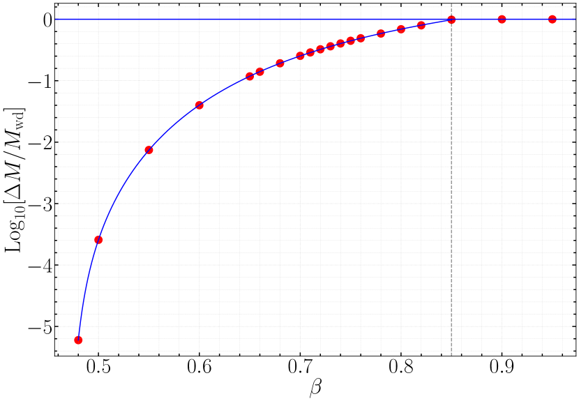
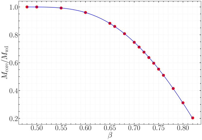
Figure 1: Left panel: Mass loss, $\Delta M$, relative to the initial WD mass, $M_{\rm wd}=1M_{\odot}$, is plotted against $\beta$. A higher $\beta$ corresponds to a stronger tidal interaction, resulting in increased mass loss. The vertical black dashed line represents $\beta_{c}=0.85$. Right panel: Variation of the final self-bound mass fraction, $M_{\rm core}/M_{\rm wd}$, with respect to $\beta$ is presented. No disruption occurs for $\beta<0.48$.

We use a fitting function inspired by Guillochon & Ramirez-Ruiz (2013) to model the variation of $\Delta M/M_{\rm wd}$ with respect to $\beta$:

$$\frac{\Delta M}{M_{\rm wd}}=\begin{cases}\exp{\Bigl{[}\frac{A+B\beta+C\beta^{2}}{1-D\beta+E\beta^{2}}\Bigr{]}}&0.48\leq\beta<0.85\\ 1.0&\beta\geq 0.85\end{cases}$$ (2)

and find the fitting parameters $A=7.6678,B=-25.7050,C=19.5925,D=5.0697$, and $E=6.2781$.

However, it is important to note that the critical impact parameter can potentially deviate from this value in the presence of various factors, such as the rotation of the star or finite temperature corrections. However, our study provides a valuable starting point for modeling the WD with this specific EOS, leaving the exploration of these corrections to $\beta_{c}$ for future work.

For comparison with Ryu et al. (2020c), where they establish the fractional remnant mass ($M_{\rm rem}/M_{\star}$) as varying with the impact parameter according to a simple functional form of $\sim 1-\beta^{3}$ for SMBH, we fit our $M_{\rm core}/M_{\rm wd}$ variation with $\beta$ using the form $1-p\beta^{q}$. The obtained variation is well modeled by $\sim 1-3.1\beta^{6.8}$. Therefore, for an IMBH with a mass of $10^{3}M_{\odot}$, one can represent the behavior as $\sim\beta^{6.8}$ when considering the variation of $\Delta M/M_{\rm wd}$ with $\beta$, while a more accurate fit is given by Equation (2).

As we determine the range of $\beta$ values where partial disruption occurs, we vary $\beta$ within the range of $0.55$ to $0.82$ and simulate partial tidal disruption. The disruptions that occur at $\beta=0.48$ and $0.50$ are very weak, and the number of particles within the bound tail is extremely low, even with an initial $10^{6}$ particles. Therefore, the fallback rate curves exhibit significant noise, and we opt not to display these plots. We continue all simulations until approximately $97\%$ to $99\%$ of the bound material has accreted onto the black hole. Finally, numerically differentiating the accreted mass with time, we calculate the fallback rate for different $\beta$ values.

It is essential to note that when calculating the fallback rate, we do not rely on the snapshot method, which has several limitations. This method involves using the energy-period relationship to predict future orbits based on early time, assuming that the debris will follow these orbits while conserving its orbital energy throughout the trajectory. However, this assumption becomes inaccurate when a self-bound core is present, and there are scenarios where the absence of a core can also lead to inaccurate results, as shown by Coughlin et al. (2016a), Coughlin et al. (2016b).

In Figure 2, the fallback rate is presented in Solar mass per hour as a function of time in hours for various $\beta$ values as mentioned in the legend. Note that the entire fallback of the bound debris occurs within a span of $\sim 100\,{\rm hrs}$, which differs from the case of SMBHs, where the fallback process takes several years to complete.

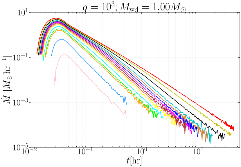
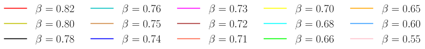
Figure 2: Fallback rates (in solar masses per hour) plotted as a function of time in hours for a $1M_{\odot}$ WD due to an IMBH in 15 different simulations. These simulations cover a range of $\beta$ values mentioned in the legend from $0.55$ to $0.82$, resulting in partial disruptions. These curves clearly demonstrate that the fallback rates asymptote to different values.

The plot clearly shows that the time at which the most bound debris falls onto the black hole increases as $\beta$ decreases from $0.82$ to $0.55$. Following the tidal interaction, a particle in the maximally deformed region of star is positioned closer to the black hole with increasing $\beta$, as it interacts at a closer $r_{p}$ position. As a result, the most bound debris follows a trajectory that returns to the black hole more quickly as $\beta$ increases. We show the trajectories of the most bound debris for three different values of $\beta=0.60,0.70$, and $0.80$ in Figure 3 Top Left, Top Right, and Bottom Left panel respectively. It is observed that with increasing $\beta$, the semi-major axis length of the most bound debris decreases, allowing it to reach the black hole more quickly. Figure 3 Bottom Right panel presents the variation of the most bound debris fallback time ($T_{\rm mb}$) with respect to $\beta$.

We also depict the relationship between $\dot{M}_{\rm max}$ (the peak of the fallback rate) and $t_{\rm max}$ (the time at which the peak occurs) with respect to $\beta$ in Figure 4 Left and Right panel respectively. It is evident that $\dot{M}_{\rm max}$ exhibits a strong dependence on $\beta$. Specifically, $\dot{M}_{\rm max,0.82}$ is approximately $\sim 38$ times that of $\dot{M}_{\rm max,0.55}$. However, the dependency of $t_{\rm max}$ on $\beta$ is relatively weak, with $t_{\rm max,0.55}$ being only about $\sim 1.4$ times that of $t_{\rm max,0.82}$.

For values of $\beta$ falling within the range of $0.65$ to $0.82$, the post-peak fallback curves exhibit an approximate scaling of $t^{-5/3}$, eventually steepening to $t^{n}$, where the exponent $n$ varies with $\beta$. Different values of $\beta$ lead to varying core masses and core-to-black hole mass ratios, defined as $\mu=M_{\rm core}/M_{\rm BH}$. In our study, $\mu$ ranges from $\sim 2\times 10^{-4}$ to $10^{-3}$, whereas for SMBHs, $\mu$ is on the order of $\sim 10^{-6}$ to $10^{-7}$. This ratio is non-negligible for IMBHs and plays a significant role in determining the late-time slope, causing a deviation from the asymptotic scaling of $t^{-9/4}$ that applies to SMBHs.

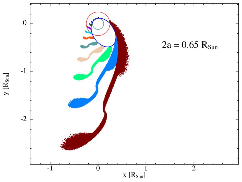
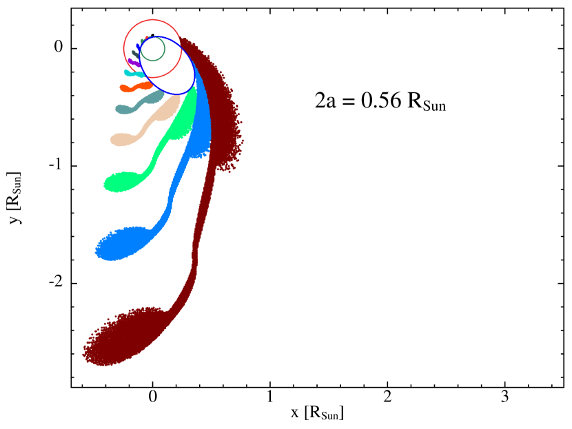
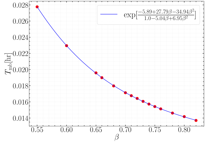
Figure 3: Top Left panel: Trajectory of the most bound debris is plotted for $\beta=0.60$. Top Right panel: Trajectory of the most bound debris is plotted for $\beta=0.70$. Bottom Left panel: Trajectory of the most bound debris is plotted for $\beta=0.80$. Here, $a$ represents the semi-major axis of the orbits, and it is observed that as $\beta$ increases, the semi-major axis length decreases. These three figures are generated using SPLASH (Price, 2007). Bottom Right panel: The variation of the time at which the most bound debris falls onto the black hole ($T_{\rm mb}$) with $\beta$ is presented. This variation is modeled by the relation mentioned in the legend.

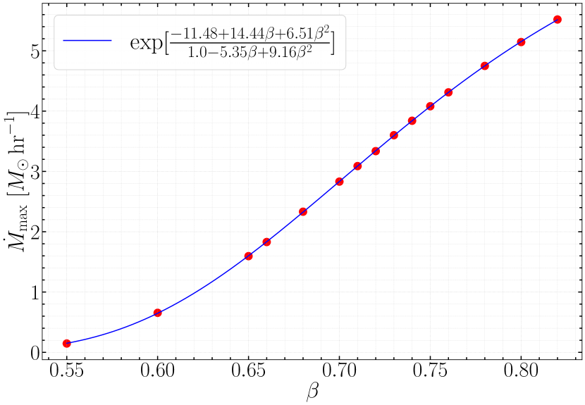
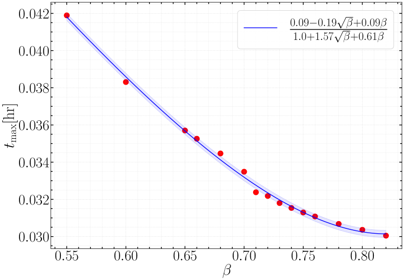
Figure 4: Left panel: Plot of $\dot{M}_{\rm max}$ as a function of $\beta$. Right panel: Plot of $t_{\rm max}$ as a function of $\beta$. As $\beta$ increases, $\dot{M}_{\rm max}$ significantly increases while $t_{\rm max}$ decreases slowly. The fitting functions are specified in the legend. The shaded blue region around the blue fitted curve represents the $1-\sigma$ deviation from the fit.

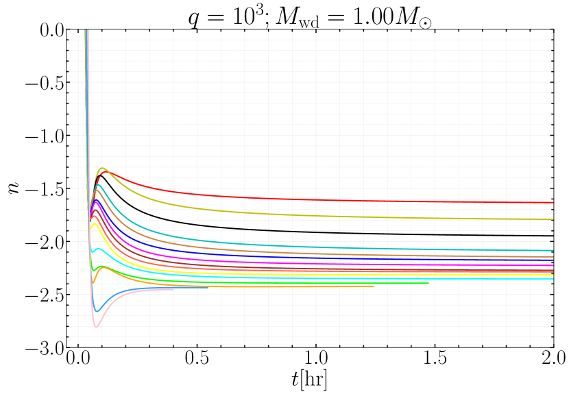
Figure 5: The instantaneous power-law index of the fallback rate, $n(t)$, is plotted against time in hours for various $\beta$ values mentioned in the legend. These plots are generated using the analytical fitting function described by Equation (3) with $N_{\rm max}=5$. It is evident that distinct $\beta$ values result in varying asymptotic power-law indices.

To accurately determine the late-time slope for different $\beta$ values, we follow the approach adopted by Nixon et al. (2021). We fit the numerically obtain fallback rate with the modified Padé approximant

$$\dot{M}_{\rm fit}=\frac{a\tilde{t}^{m}}{1+\frac{a}{b}\tilde{t}^{m-n_{\infty}}}\frac{1+\Sigma_{i=1}^{N_{\rm max}-1}c_{i}\tilde{t}^{i}+\tilde{t}^{N_{\rm max}}}{1+\tilde{t}^{N_{\rm max}}}$$ (3)

Here, we introduce a normalized time variable, $\tilde{t}=t/t_{\rm max}$. This choice of analytical function, as suggested by Nixon et al. (2021), is based on the observation that the initial rise before the peak and the late-time decay are effectively described by the functional form $a\tilde{t}^{m}/(1+\frac{a}{b}\tilde{t}^{m-n_{\infty}})$, where $\tilde{t}^{m}$ and $\tilde{t}^{n_{\infty}}$ represent power-law behaviors for the initial rise and late-time decay, respectively. The phase in between is accurately described by the ratio of polynomials, known as the Padé approximant. To determine the values of the constants $a,b,m,n_{\infty},c_{1},c_{2},...,c_{N_{\rm max}-1}$, we minimize the chi-square defined as

$$\chi^{2}=\sum_{i}\Bigg{(}{\rm{ln}}\Big{(}\frac{\dot{M}_{i}}{\dot{M}_{\rm halfmax}}\Big{)}-{\rm{ln}}\Big{(}\frac{\dot{M}_{\rm fit}(\tilde{t}_{i})}{\dot{M}_{\rm halfmax}}\Big{)}\Bigg{)}^{2}$$ (4)

Here, we define $\dot{M}_{\rm halfmax}$ as half of $\dot{M}_{\rm max}$, and $\dot{M}_{i}$ represents the numerically determined fallback rate at $\tilde{t}_{i}$. We tested the analytical fit using a range of terms, from $N_{\rm max}=5$ to $10$. Our findings indicate that increasing the number of terms in the numerator of Equation (3) does not significantly alter the characteristics of the curves. Moreover, the chi-square value does not decrease significantly when $N_{\rm max}>5$. Therefore, we chose to use $N_{\rm max}=5$ to model the fallback curves for different $\beta$ values. Once we obtain the analytical fits, we can determine the relationship between the power-law index and time using the simple relation $\dot{M}\propto t^{n}$, where $n(t)=d(\log{\dot{M}})/d(\log t)$. In Figure 5, we depict the variation in the power-law index over time in hours. It becomes evident from the figure that the late-time behavior of the power-law index ($n_{\infty}$) for the fallback rates with surviving cores does not asymptote to the well-established value of $-9/4$ for SMBHs.

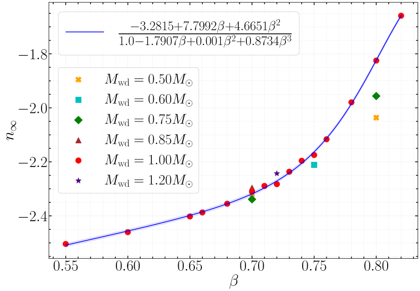
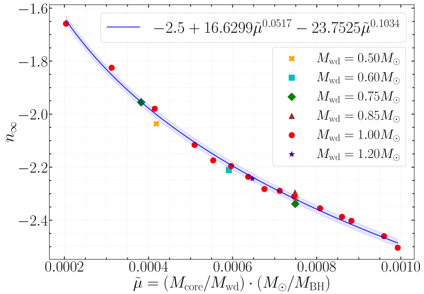
Figure 6: Left panel: The late-time power-law index, $n_{\infty}$, is plotted as a function of $\beta$. Right panel: The late-time power-law index, $n_{\infty}$, is depicted as a function of $\tilde{\mu}=(M_{\rm core}/M_{\rm wd})\cdot(M_{\odot}/M_{\rm BH})$. The shaded blue region around the blue fitted curve represents the $1-\sigma$ deviation from the fit.

We observe variations in $n_{\infty}$ for different $\beta$ values, ranging from $-1.66$ to $-2.50$ as $\beta$ decreases from $0.82$ to $0.55$. As core mass and $\mu$ both increase with decreasing $\beta$, the influence of the core on the falling material becomes more pronounced, leading to a deviation of $n_{\infty}$ from the value $-9/4$. In Figure 6, we present the variation of $n_{\infty}$ with $\beta$. We fit $n_{\infty}$ with respect to $\beta$, which is expressed as:

$$n_{\infty}=\frac{-3.2815+7.7992\beta+4.6651\beta^{2}}{1-1.7907\beta+0.001\beta^{2}+0.8734\beta^{3}}.$$ (5)

We performed an additional set of $7$ simulations, systematically varying the initial WD mass and $\beta$ to assess the influence of changing stellar structure on $n_{\infty}$. The initial WD mass varies from $0.50M_{\odot}$ to $1.20M_{\odot}$, as indicated in the legend of Figure 6. We observe that $n_{\infty}$ exhibits notable variations with initial WD masses for higher $\beta$. For instance, with $\beta=0.70$ and initial WD masses of $0.50M_{\odot}$ and $1.00M_{\odot}$, we obtain $n_{\infty}$ values of $-2.32$ and $-2.31$, respectively. In contrast, for $\beta=0.80$ with the same masses, $n_{\infty}$ becomes $-2.04$ and $-1.82$, respectively. This variation arises from the different amount of disruption observed for a fixed $\beta$ with different initial WD masses, and this discrepancy becomes more pronounced with increasing $\beta$. For an initial WD mass of $0.50M_{\odot}$, the ratio of disrupted mass and the initial WD mass $\Delta M/M_{\rm wd}$ at $\beta=0.70$ and $0.80$ is $0.25$ and $0.58$, respectively, while for $1.00M_{\odot}$, these values are $0.25$ and $0.69$. Note that in the literature, typically the late time slope is studied as a function of the variable $\mu=M_{\rm core}/M_{\rm BH}$. This variable however does not contain any information about the WD mass, since WDs with different masses and different impact parameters can result in the same mass of the remnant core. Hence to make a more robust comparison of the late-time slopes for TDEs of different WDs in the same BH background, we introduce a variable $\tilde{\mu}=(M_{\rm core}/M_{\rm wd})\cdot(M_{\odot}/M_{\rm BH})$. In Figure 6, we present the variation in $n_{\infty}$ with respect to $\tilde{\mu}$. We fit the relationship between $n_{\infty}$ and $\tilde{\mu}$ and provide the fitting formula as follows :

$$n_{\infty}=-2.5+16.6299\tilde{\mu}^{0.0517}-23.7525\tilde{\mu}^{0.1034}.$$ (6)

We studied partial disruption for 5 more WDs characterized by initial masses different from $1.00M_{\odot}$ (see Figure 6). We see that the relationship between $n_{\infty}$ and $\tilde{\mu}$ closely matches the behaviour predicted by the fitting formula. It’s noteworthy that all data points fall within the $3-\sigma$ range of the fitting formula, affirming the accuracy of the same.

4 Discussion and Summary

In this paper, we have studied partial TDEs, where an initial spherical WD in a parabolic orbit is partially disrupted by an IMBH. We have presented results of 22 numerical simulations. In 15 of these, we considered a solar mass WD, and studied partial TDEs by varying the impact parameter $\beta$; and in the other 7 simulations, different WD masses were considered at particular values of $\beta$. We employed the zero temperature EOS directly in the SPH code to model the WDs, and finite temperature corrections have been neglected, as the central density of the initial WDs is $\sim 10^{7}\,\text{g}\,\text{cm}^{-3}$. For solar mass WDs, we determined the range of $\beta$ for which partial disruptions occur, using this EOS, and this gives $0.48\leq\beta<0.85$. We note that this range may be altered due to several factors, e.g., rotation of the initial WD which might modify our analysis, and we leave this issue for a separate study.

We have calculated the fallback rates numerically for the partial TDEs using impact parameters ranging from $\beta=0.55$ to $\beta=0.82$, corresponding to pericenter positions from $70r_{g}$ to $47r_{g}$, where $r_{g}$ is the gravitational radius. According to Tejeda et al. (2017), relativistic effects may be significant for $r_{p}\lesssim 10r_{g}$. Therefore, in our study, we have safely neglected relativistic corrections. We have observed that with increasing $\beta$, the time of return of the most bound debris decreases. Additionally, we observe that the peak of the fallback rate strongly depends on $\beta$, increasing with higher values of $\beta$. However, the time at which the peak occurs only exhibits weak dependence on $\beta$ : as $\beta$ decreases, this time increases. Notably, we find here that the late-time power-law index does not asymptote to the usual $-9/4$ scaling, which is well known for partial TDEs due to SMBHs. We have found that $n_{\infty}$ varies from $-5/3$ for full disruption to $-2.50$ for $\beta=0.55$. This variation is due to the differing core masses for various $\beta$ values, and the ratio of the core mass to the black hole mass, although small, is not negligible, as is the case for SMBHs. This factor plays a significant role in determining $n_{\infty}$. Furthermore, we have found a robust fitting formula for the late time power law of the fallback rate (denoted by $n_{\infty}$) with the parameter $\tilde{\mu}=(M_{\rm core}/M_{\rm wd})\cdot(M_{\odot}/M_{\rm BH})$. Performing 7 simulations with initial WD mass other than $1M_{\odot}$, we find that our formula accurately predicts the late time fall back rate, independent of the WD mass, i.e., the obtained values fall within the $3-\sigma$ limit of the fitting formula. Changing the mass of the central black hole alters this formula, and issue that we have not delved into.

We believe that the observational aspect of our study could be significant, since the fallback rate is expected to closely track the accretion rate. We have highlighted important differences of the physics of TDEs in the background of IMBHs as compared to SMBHs, and our results could serve as a robust criterion in the detection of IMBHs via TDEs, since deviations in the light curves from the expected $-9/4$ scaling could serve as a promising indicator for the presence of IMBHs.

Acknowledgements

We acknowledge the support and resources provided by PARAM Sanganak under the National Supercomputing Mission, Government of India, at the Indian Institute of Technology Kanpur. The work of DG is supported by grant number 09/092(1025)/2019-EMR-I from the Council of Scientific and Industrial Research (CSIR). The work of TS is supported in part by the USV Chair Professor position at IIT Kanpur, India.

References

- Abbott et al. (2020) Abbott, R., Abbott, T. D., Abraham, S., et al. 2020, Phys. Rev. Lett., 125, 101102. doi:10.1103/PhysRevLett.125.101102
- Balsara (1995) Balsara, D. S. 1995, Journal of Computational Physics, 121, 357. doi:10.1016/S0021-9991(95)90221-X
- Banerjee et al. (2023) Banerjee, P., Garain, D., Chowdhury, S., et al. 2023, MNRAS, 522, 4332. doi:10.1093/mnras/stad1284
- Bonnerot et al. (2016) Bonnerot, C., Rossi, E. M., Lodato, G., et al. 2016, MNRAS, 455, 2253. doi:10.1093/mnras/stv2411
- Brown et al. (2015) Brown, G. C., Levan, A. J., Stanway, E. R., et al. 2015, MNRAS, 452, 4297. doi:10.1093/mnras/stv1520
- Carter & Luminet (1982) Carter, B. & Luminet, J. P. 1982, Nature, 296, 211. doi:10.1038/296211a0
- Carter & Luminet (1983) Carter, B. & Luminet, J.-P. 1983, A&A, 121, 97
- Chen & Shen (2018) Chen, J.-H. & Shen, R.-F. 2018, ApJ, 867, 20. doi:10.3847/1538-4357/aadfda
- Chen et al. (2023) Chen, J.-H. Shen, R.-F. & Liu S-F., ApJ, 947, 32. doi:10.3847/1538-4357/acbfb6
- Chilingarian et al. (2018) Chilingarian, I. V., Katkov, I. Y., Zolotukhin, I. Y., et al. 2018, ApJ, 863, 1. doi:10.3847/1538-4357/aad184
- Clerici & Gomboc (2020) Clerici, A. & Gomboc, A. 2020, A&A, 642, A111. doi:10.1051/0004-6361/202037641
- Coughlin & Nixon (2015) Coughlin, E. R. & Nixon, C. 2015, ApJ, 808, L11. doi:10.1088/2041-8205/808/1/L11.
- Coughlin et al. (2016a) Coughlin, E. R., Nixon, C., Begelman, M. C., et al. 2016a, MNRAS, 455, 3612. doi:10.1093/mnras/stv2511
- Coughlin et al. (2016b) Coughlin, E. R., Nixon, C., Begelman, M. C., et al. 2016b, MNRAS, 459, 3089. doi:10.1093/mnras/stw770
- Coughlin & Nixon (2019) Coughlin, E. R. & Nixon, C. J. 2019, ApJ, 883, L17. doi:10.3847/2041-8213/ab412d
- Cufari et al. (2022) Cufari, M., Coughlin, E. R., & Nixon, C. J. 2022, ApJ, 924, 34. doi:10.3847/1538-4357/ac32be
- Darbha et al. (2019) Darbha, S., Coughlin, E. R., Kasen, D., et al. 2019, MNRAS, 488, 5267. doi:10.1093/mnras/stz1923
- Evans & Kochanek (1989) Evans, C. R. & Kochanek, C. S. 1989, ApJ, 346, L13. doi:10.1086/185567
- Frank & Rees (1976) Frank, J. & Rees, M. J. 1976, MNRAS, 176, 633. doi:10.1093/mnras/176.3.633
- Gafton et al. (2015) Gafton, E., Tejeda, E., Guillochon, J., et al. 2015, MNRAS, 449, 771. doi:10.1093/mnras/stv350
- Gafton & Rosswog (2019) Gafton, E. & Rosswog, S. 2019, MNRAS, 487, 4790. doi:10.1093/mnras/stz1530
- Garain et al. (2023) Garain, D., Banerjee, P., Chowdhury, S., et al. 2023, arXiv:2307.03142. doi:10.48550/arXiv.2307.03142
- Golightly et al. (2019a) Golightly, E. C. A., Nixon, C. J., & Coughlin, E. R. 2019a, ApJ, 882, L26. doi:10.3847/2041-8213/ab380d
- Golightly et al. (2019b) Golightly, E. C. A., Coughlin, E. R., & Nixon, C. J. 2019b, ApJ, 872, 163. doi:10.3847/1538-4357/aafd2f
- Greene et al. (2020) Greene, J. E., Strader, J., & Ho, L. C. 2020, ARA&A, 58, 257. doi:10.1146/annurev-astro-032620-021835
- Guillochon & Ramirez-Ruiz (2013) Guillochon, J. & Ramirez-Ruiz, E. 2013, ApJ, 767, 25. doi:10.1088/0004-637X/767/1/25
- Guillochon et al. (2014) Guillochon, J., Manukian, H., & Ramirez-Ruiz, E. 2014, ApJ, 783, 23. doi:10.1088/0004-637X/783/1/23
- Hayasaki et al. (2013) Hayasaki, K., Stone, N., & Loeb, A. 2013, MNRAS, 434, 909. doi:10.1093/mnras/stt871
- Hayasaki et al. (2016) Hayasaki, K., Stone, N., & Loeb, A. 2016, MNRAS, 461, 3760. doi:10.1093/mnras/stw1387
- Hills (1975) Hills, J. G. 1975, Nature, 254, 295. doi:10.1038/254295a0
- Holoien et al. (2019) Holoien, T. W.-S., Vallely, P. J., Auchettl, K., et al. 2019, ApJ, 883, 111. doi:10.3847/1538-4357/ab3c66
- Jonker et al. (2022) Jonker, P. G, Arcavi, I., Phinney, E. S, et al. 2022, The Tidal Disruption of Stars by Massive Black Holes (Springer)
- Kagaya et al. (2019) Kagaya, K., Yoshida, S., & Tanikawa, A. 2019, arXiv:1901.05644. doi:10.48550/arXiv.1901.05644
- Kızıltan et al. (2017) Kızıltan, B., Baumgardt, H., & Loeb, A. 2017, Nature, 542, 203. doi:10.1038/nature21361
- Kochanek (1994) Kochanek, C. S. 1994, ApJ, 422, 508. doi:10.1086/173745
- Lacy et al. (1982) Lacy, J. H., Townes, C. H., & Hollenbach, D. J. 1982, ApJ, 262, 120. doi:10.1086/160402
- Law-Smith et al. (2017) Law-Smith, J., MacLeod, M., Guillochon, J., et al. 2017, ApJ, 841, 132. doi:10.3847/1538-4357/aa6ffb
- Law-Smith et al. (2019) Law-Smith, J., Guillochon, J., & Ramirez-Ruiz, E. 2019, ApJ, 882, L25. doi:10.3847/2041-8213/ab379a
- Law-Smith et al. (2020) Law-Smith, J. A. P., Coulter, D. A., Guillochon, J., et al. 2020, ApJ, 905, 141. doi:10.3847/1538-4357/abc489
- Lin et al. (2020) Lin, D., Strader, J., Romanowsky, A. J., et al. 2020, ApJ, 892, L25. doi:10.3847/2041-8213/ab745b
- Liptai et al. (2019) Liptai, D., Price, D. J., Mandel, I., et al. 2019, arXiv:1910.10154. doi:10.48550/arXiv.1910.10154
- Lodato et al. (2009) Lodato, G., King, A. R., & Pringle, J. E. 2009, MNRAS, 392, 332. doi:10.1111/j.1365-2966.2008.14049.x
- MacLeod et al. (2013) MacLeod, M., Ramirez-Ruiz, E., Grady, S., et al. 2013, ApJ, 777, 133. doi:10.1088/0004-637X/777/2/133
- Mainetti et al. (2017) Mainetti, D., Lupi, A., Campana, S., et al. 2017, A&A, 600, A124. doi:10.1051/0004-6361/201630092
- Manukian et al. (2013) Manukian, H., Guillochon, J., Ramirez-Ruiz, E., et al. 2013, ApJ, 771, L28. doi:10.1088/2041-8205/771/2/L28
- Miles et al. (2020) Miles, P. R., Coughlin, E. R., & Nixon, C. J. 2020, ApJ, 899, 36. doi:10.3847/1538-4357/ab9c9f
- Nixon et al. (2021) Nixon, C. J., Coughlin, E. R., & Miles, P. R. 2021, ApJ, 922, 168. doi:10.3847/1538-4357/ac1bb8
- Park & Hayasaki (2020) Park, G. & Hayasaki, K. 2020, ApJ, 900, 3. doi:10.3847/1538-4357/ab9ebb
- Phinney (1989) Phinney, E. S. 1989, The Center of the Galaxy, 136, 543
- Price (2007) Price, D. J. 2007, PASA, 24, 159. doi:10.1071/AS07022
- Rees (1988) Rees, M. J. 1988, Nature, 333, 523. doi:10.1038/333523a0 .
- Ryu et al. (2020a) Ryu, T., Krolik, J., Piran, T., et al. 2020a, ApJ, 904, 98. doi:10.3847/1538-4357/abb3cf
- Ryu et al. (2020b) Ryu, T., Krolik, J., Piran, T., et al. 2020b, ApJ, 904, 100. doi:10.3847/1538-4357/abb3ce
- Ryu et al. (2020c) Ryu, T., Krolik, J., Piran, T., et al. 2020c, ApJ, 904, 100. doi:10.3847/1538-4357/abb3ce
- Sacchi & Lodato (2019) Sacchi, A. & Lodato, G. 2019, MNRAS, 486, 1833. doi:10.1093/mnras/stz981
- Takekawa et al. (2019) Takekawa, S., Oka, T., Iwata, Y., et al. 2019, ApJ, 871, L1. doi:10.3847/2041-8213/aafb07
- Tejeda et al. (2017) Tejeda, E., Gafton, E., Rosswog, S., et al. 2017, MNRAS, 469, 4483. doi:10.1093/mnras/stx1089
- Tejeda & Rosswog (2013) Tejeda, E. & Rosswog, S. 2013, MNRAS, 433, 1930. doi:10.1093/mnras/stt853
- Open TDE Catalog (2023) The Open TDE Catalog, 2023, available at https://tde.space/
- Ulmer (1999) Ulmer, A. 1999, ApJ, 514, 180. doi:10.1086/306909.
- Volonteri (2012) Volonteri, M. 2012, Science, 337, 544. doi:10.1126/science.1220843
- Wang et al. (2021) Wang, Y.-H., Perna, R., & Armitage, P. J. 2021, MNRAS, 503, 6005. doi:10.1093/mnras/stab802.