Inverse design of self-folding 3D shells

Abstract

Inverse design aims at the development of elementary building blocks that organize spontaneously into target shapes. In self-assembly, the blocks diffuse to their target position. Alternatively, recent experiments point to a more robust process in which the shape is formed from the self-folding of a planar template. To control the folding of templates with competing folded structures, we propose the inclusion of bond specificity. We consider a template that can fold into an octahedron or a boat shell and find the minimal design capable of targeting either shell or switching between the two through an external stimulus, adding a new dimension to the design of shape-changing materials.

The ability to externally control the formation of microscopic structures and to selectively switch between different conformations are among of the most ambitious goals of materials design  [1, 2, 3]. One of the most successful paradigms for the bottom-up realization of ordered aggregates, from the molecular to the colloidal scale, is self-assembly [4, 5, 6]. In this process, a dispersion of building blocks aggregate due to carefully designed attractive (or entropic [7]) interactions. Despite its potential, self-assembly is inherently limited by the kinetics of the aggregation process, and is often derailed by the presence of kinetic intermediate structures whose long lifetime prevents the correct assembly of the target structure [8, 9, 10].

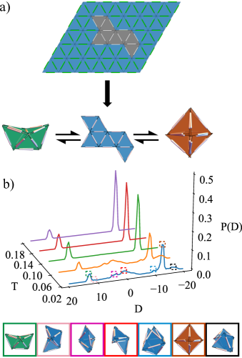
Figure 1: a) Schematic representation of a triangular tiling of 2D space, where the net studied (in white) can be cut. Below are shown the two possible structures formed by folding this specific planar net (middle). On the left is the octahedron while on the right is the boat. The rods on the edges are only used for visualization purposes. b) Histogram of the order parameter for different temperatures. Below the histogram are represented the most probable misfoldings with a color scheme corresponding to the points highlighted in the histogram. These results were averaged over 1000 samples.

Inspired by the tremendous progress of DNA nanotechnology in general and DNA origami in particular, here we investigate an alternative route to self-assembly, represented by self-folding materials, i.e. 2D planar templates (nets) that are designed to fold into the desired structure [11, 12]. Compared to traditional self-assembly methods, self-folding has some key advantages: i) it can be triggered on faster time-scales compared to self-assembly, as the different units do not need to explore the volume of the system to assemble; ii) its basic units, the tiles, are generally simpler to realize, as one needs only to consider planar interactions, compared to the complex three-dimensional building blocks required for self-assembly; iii) it holds the promise to realize shape-shifting materials, as self-folding can easily adapt to changing external conditions, contrary to the structures obtained by self-assembly which are difficult to reconfigure without disassembling and reassembling the components.

Experimentally, DNA-origami have made the biggest contribution towards fully realizing the potential of self-folding systems thanks to their nanoscale precision, geometric design, and the fully-controllable specificity of the base pairing. Moreover, they allow for selective interactions between elementary constituents through different energy scales, by tuning DNA chain length [13]. Application to produce controllable planar nets have seen a rapid growth in recent years, and include so called DNA kirigami [14], DNA origami tesselations [15], and recently introduced reconfigurable (akin to paper-folding mechanism) planar DNA origami [12], to name a few. Additionally, new micron-sized planar structures based on seeded assembly of DNA origami criss-cross slats [16] would present a new potential way to create larger shape- shifting 3D nanostructures folded from 2D planar template. The folding of 2D planar templates has also gathered a lot of theoretical interest, especially as a means of assembling 3D capsules or shells [17]. Given that the phase space of structures that can be folded is finite and well-known [18] it is the folding pathway that dictates the final structure. Control over the folding pathways for single [19, 20] and multiple targets [21] have so far focused on the influence of the network topology on the final assembled structure [8].

In this work we propose a novel way to control the folding pathway of 2D planar nets based on bond specificity between the edges of the tiles that compose the net. Our goal is to enhance and/or selectively steer the folding process by optimizing the interaction between the edges for any given net. These interactions are designed with an inverse design method called SAT-assembly [22], which translates the topologies of the 3D target shells into a Boolean Satisfiability Problem (SAT), where the design problem is formulated in terms of binary variables and logic clauses, for which fast solution methods are available [23] . To demonstrate our approach we focus on a prototypical example of self-folding net, shown in Fig. 1, which is composed of eight faces, all being equilateral triangles of the same size. The net can fold into two ordered 3D shells, the octahedron and the boat, and a large variety of disordered structures.

Each triangular face of the net represents a tile, where edges between tiles can interact attractively. The interactions can be represented as colors, such that two edges interact according to a color interaction matrix. This coloring is subject to multiple constraints. Firstly, we require the nets to be able to tile the plane, so that one can first create a 2D triangular lattice with the respective tiles and then cut the final net to fold the 3D shell; this condition mimics standard experimental methods where a plane is first seeded on a 2D substrate and then the final net is etched from it [24]. Secondly, we want the net to fold in either the boat or octahedron configurations [2, 21]. Alternatively, we want to be able to change the target structure depending on the external conditions, i.e. create reconfigurable shape-shifting structures.

To tackle the computational complexity imposed by these conditions, we cast the folding process as a SAT problem as follows. We consider that each edge can be attributed a color $x_{c}\in\{1,2,...,N_{c}\}$, where $N_{c}$ is the total number of distinct colors used among all tiles. The tile type $x_{p}$ is specified by the color arrangement of its edges, with each unique combination representing a different type $x_{p}\in\{1,2,...,N_{p}\}$, where $N_{p}$ is the total number of different tile types. $N_{c}$ and $N_{p}$ are the input parameters. We then use a SAT solver [23] to find the tile coloring with $N_{c}$ colors and $N_{p}$ types that satisfies all the constraints. In the following, we will show results for the system of Fig. 1. In the Supplementary Material we go into more detail on the constraints (clauses) used in SAT.

To verify the folding pathways we run molecular dynamics simulations of the self-folding process. To simulate the tiles, we introduce a patchy particle model, where each face is represented by a hard core tiny sphere of radius of only $0.3$, in units of length corresponding to the distance from the center of each tile to any of its edges ($\sigma$). Chosen to keep steric effects to a minimum while preventing the faces from overlapping with each other. Two attractive patches are located on each edge, at equidistant points from the center of the edge. This number of patches per edge is the minimum to allow for the faces to hinge. The patches have an attractive isotropic point potential to describe the attractive interactions between the edges. If two patches are within a range of $\delta=0.18$, and if they are of the same color, they form a bond of energy $\varepsilon$ (our energy unit). The internal edges of the net (the ones that start bonded) interact with an energy of $5\,\varepsilon$, so that they never break for the range of temperatures explored in this work. In the Supplementary Material we go into more detail on the potentials used for the interactions. We perform Brownian Dynamics simulations of our model using the oxDNA package [25]. The particle system was simulated using rigid-body molecular dynamics with an Andersen-like thermostat [26]. Temperature is measured in units of $\epsilon/k_{B}$, where $k_{B}$ is the Boltzmann constant. We always start from the same initial configuration which corresponds to the net shown in Fig. 1 and run the simulations for a maximum of $10^{9}$ timesteps, with each step corresponding to $\Delta t=0.001$, in units of $\sigma/\sqrt{m/\varepsilon}$, where $m$ is the mass of each individual tile. During the simulation, each patch on the edge was only able to bind to one other at a time. All results are averaged over 1000 independent simulations.

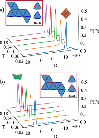
Figure 2: Histograms of the order parameter as a function of temperature for two different designs. Plot a) corresponds to the net which excludes the boat. Plot b) corresponds to a net which excludes the octahedron. The respective designs are highlighted by the red box, which includes the net, the different tiles used and the interaction matrix between the colors. Both nets only use 2 different tile types and 2 colors total (N2c2). All results were averaged over 1000 samples.

We first consider a net where all edges have the same color that binds to itself, as shown in Fig. 1. We refer to this design as N1C1 (one tile type and one color). Given that we always start with the same net, there is only one possible combination for bonding between patch pairs ($pp$) that closes either the octahedron ($O$) or the boat ($B$). We can create the contact network for either structure, which includes the respective patch pairs, and check, after folding, if the shell formed satisfies either one structure or the other. To properly identify the different shells, we introduce an order parameter based on the distance between pairs of patches:

$$D=D_{\rm octahedron}-D_{\rm boat}=\sum_{pp\in O}r_{ij}-\sum_{pp\in B}r_{ij}\ ,$$ (1)

where $D_{\rm octahedron}$ is equal to the sum of the distances ($r_{ij}$) between all patch pairs in the octahedron contact network, while $D_{\rm boat}$ is equal to the sum of the distances between all patch pairs in the boat contact network. Thus, if a net folds a boat, $D_{\rm boat}\ll D_{\rm octahedron}$ and $D$ is largely positive, while if it folds an octahedron, $D_{\rm octahedron}\ll D_{\rm boat}$ and $D$ is largely negative. The order parameter also gives information if a given misfolded shell is closer to the octahedron or the boat. In Fig. 1b we show a histogram of the order parameter for different temperatures. In the snapshots we highlight the octahedron, the boat, and the most probable misfolded shells observed as peaks in the order parameter distribution. We observe that at low temperatures the system often gets trapped in misfolded configurations. As temperature is increased, thermal fluctuations allow the system to find the two free energy minima corresponding to the boat and octahedron configurations. From the height of the peaks, we observe that the octahedron is the kinetically preferred structure for this model, even if both the octahedron and boat have the same number of bonds and, thus, the same energy. The results of Fig. 1 highlight the biggest problem with generic self-folding systems: the presence of multiple local minima that can significantly reduce the yield of the final structure, especially at low temperatures, where the aggregates are kinetically stabilized.

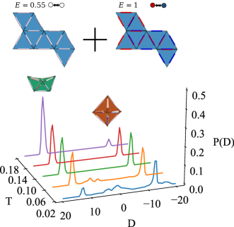
Figure 3: On top are shown the two nets that compete to fold the structures. The net with the lowest bond energy corresponds to the one tile type and one color design (N1C1) while the highest energy net corresponds to the two tile types and two colors design (N2C2) which excludes the octahedron, shown in Fig. 2, right column. If two tiles meet which form a white-white bond then the energy of the bond will be almost half of the reference bond energy, while if a red-blue bond can be formed, it will have the reference bond energy. Below is shown the histogram of the order parameter for different temperatures. Results were averaged over 1000 samples.

In Fig. 2 we show the effect of using colored designs, using SAT to find a minimum combination of tile types that satisfies only one of the structures while avoiding the other. For both structures, we find that the minimum design requires two different tile types and two colors (N2c2). In the left column is a design that folds the octahedron while avoiding the boat. The interaction matrix between the colored edges is also shown. Particularly, if an edge with the color red finds another with the color blue they interact as before, while if both edges have the same color the interaction energy is zero. In the results below, we confirm that the probability of finding the boat is always zero. On the right column is a design that folds the boat while excluding the octahedron, as confirmed by the order parameter histograms. The histograms show that this coloring strategy is not only effective at selecting the intended designs but also at suppressing disordered kinetic aggregates. As the specificity of the interactions increases, it is less probable that a bond not present in the final structure is formed. Increasing the total number of colors/tile types is thus a viable strategy to increase the success probability of the folding process.

So far, we have used designs that target a specific structure while avoiding competing ones [27, 28]. We now show how to use the designs produced by SAT to target multiple structures. For that, it is sufficient to linearly combine the interaction matrices of two designs that target different structures. The coefficients of this linear combination express the relative strength of the bonds in one of the structures compared to the others. For example, we can use two designs, the N1C1 (Fig. 1) and the N2C2 (Fig. 2 right column), and assign their respective interaction matrices different energy values. Since the octahedron is more probable in the N1C1 design, we assign a higher energy value to the N2C2 design which only forms the boat. This means that the minima corresponding to the boat will be deeper and thus more energetically favored, while the dynamical pathways will favor the octahedron, as noted previously. With this method, if two edges with interacting colors according to the N2C2 design meet, they form a bond with energy $\varepsilon=1$. If they do not interact according to the N2C2 design, then they will interact only through the N1C1 design and have energy $E_{r}\leq 1$.

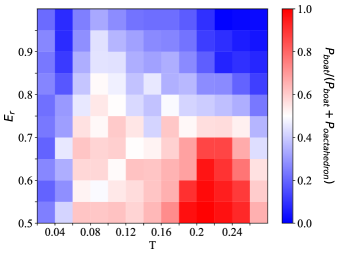
Figure 4: Fraction of boats formed between all closed structures for different temperatures and $E_{r}$. The designs used correspond to the ones shown in Fig. 3. The colormap is calculated for each state point as $P_{boat}/(P_{boat}+P_{octahedron})$, where $P_{x}$ corresponds to the probability of folding a given structure. Results were averaged over 100 samples.

In Fig. 3 we show the two nets used with their respective coloring and the respective energies. We also show the order parameter histogram for different temperatures. Here, we compare the folding of the boat and octahedron for $E_{r}=0.55$ (see Supplementary Material for other results). We observe that, at lower values of temperature, the results are quite similar to the N1C1 shown in Fig. 1, where the octahedron is the most probable structure. Given that the temperature is lower, the folding process can get stuck in local minima for longer. Since the octahedron pathway is more probable than the boat, this shell will fold more frequently and due to the low temperatures remain stuck in this state. At higher values of temperature, the boat eventually becomes the most probable structure. Since the bonds break more frequently, the net will more quickly reach the global energy minimum (boat), which becomes more and more favored as $E_{r}$ decreases. Thus, we find that by introducing the two competing designs with relative energies one can favor different shells at opposite temperature ranges. In Fig. 4 we show a diagram of the parameter space for different $E_{r}$ and temperatures. The colormap indicates the fraction of boats formed and is calculated using $P_{boat}/(P_{boat}+P_{octahedron})$, where $P_{x}$ corresponds to the probability of folding a given structure. The diagram shows that the free energy minimum associated with the boat configuration becomes dominant for $E_{r}\leq 0.7$, where the shape-shift between the octahedron and the boat can be controlled by varying the temperature.

To conclude, we have shown how specific (colored) interactions can greatly improve the self-folding yield, and how several important properties can be embedded into the design via satisfiability methods. These allow us to suppress unwanted structures at the expense of a minimal increase in complexity. For example, in the case of a net that can fold into both the icosahedron and boat configurations, we have shown that going from a 1-component (with one tile type) to a 2-component (two different tile types) is sufficient to reach an almost perfect yield of either structure. We have then introduced the idea of linearly combining different designs to achieve external control over the final structure. In our case, we can change the ratio between the octahedron and the boat by changing the temperature. This highlights SAT-assembly of 2D planar nets not only as a method to avoid competing structures but also as a possible way to develop new shape shifting materials. With recent experimental advancements in DNA-origami nanotechnology, self-folding holds the potential to find wide application in the assembly of reconfigurable systems. A foldable 2D template can be achieved from a single DNA origami [12], or from multiple DNA origami nanostructures connected [16, 29]. The edges can then be functionalized with single-stranded DNA overhangs that will act as bonds between edges, with specificity and interaction strength given by the interaction matrix from our SAT-assembly approach. In this context, the SAT-assembly approach is a promising step towards programming variable shapes directly into the structure. It is possible to use our method to store multiple structures in a single 2D net thus enabling potential experimental realization of shape-shifting nanostructures that have multiple stable folds that can be selectively recalled [30, 31]. They can be designed to switch conformation at e.g. at different temperatures, or due to an external stimulus, such as the presence of single-stranded DNA detectors that can strengthen the interaction between specific edges that will drive the rest of the structure to refold [12, 32].

Supplementary Materials

.1 Simulation model details

In the molecular dynamics simulations we use oxDNA [25] to simulate a patchy particle model with a point patch potential. Each particle is comprised of 6 patches at positions, $\textbf{p}_{1}=(0.433,0.5,0)$, $\textbf{p}_{2}=(-0.433,0.5,0)$, $\textbf{p}_{3}=(-0.65,0.125,0)$, $\textbf{p}_{4}=(-0.217,0.625,0)$, $\textbf{p}_{5}=(0.65,0.125,0)$, and $\textbf{p}_{6}=(0.217,-0.625,0)$, respective to the center of mass of the patchy particle. These positions ensure that there are 2 patches per edge of the abstract triangle face inscribed on the particle, at equal distance from the center of the respective edge.

The point patch potential is similar to the one used in Ref. [27], where the interaction between patches $a$ and $b$ of particles $i$ and $j$, is given by:

$$V_{patch}(r_{ij})=\delta_{ab}V_{pdist}(r_{p}),$$ (S1)

where $\delta_{ab}$ is $E$ if $a$ and $b$ have colors which interact, otherwise it is 0. The distance part of the potential $V_{pdist}$ is given by:

$$V_{pdist}(r_{p})=\left\{\begin{array}[]{l l}-1.001\exp{\big{[}-\big{(}\frac{r_{p}}{\alpha}\big{)}^{10}\big{]}}+C&r_{p}\leq r_{pmax}\\ 0&\text{otherwise}\end{array}\right.$$ (S2)

Thus, $r_{p}$ is the distance between the patches and $\alpha$ sets the patch width, which we fix at $\alpha=0.12$. The constant $C$ is set so that $V_{patch}(r_{pmax})=0$ for $r_{pmax}=0.18$. The centers of the patchy particles interact through an excluded volume interaction

$$f_{exc}(r,\sigma,r^{*})=\left\{\begin{array}[]{l l}V_{LJ}(r,\sigma)&r<r^{*},\\ V_{smooth}(r,b,r^{c})&r^{*}<r<r^{c}\\ 0&\text{otherwise}\\ \end{array}\right.$$ (S3)

Here, $r$ is the distance between the centers of mass of the patchy particles, and $\sigma=1.0$ corresponding to the distance from the center of each tile to any of its edges. Then, $V_{LJ}$ is the Leonnard-Jonnes potential:

$$V_{LJ}(r,\sigma)=8\bigg{[}\bigg{(}\frac{\sigma}{r}\bigg{)}^{12}-\bigg{(}\frac{\sigma}{r}\bigg{)}^{6}\bigg{]}$$ (S4)

which is truncated using a quadratic smoothing function:

$$V_{smooth}(x,b,x_{c})=b(x_{c}-x)^{2}$$ (S5)

where $b$ and $x_{c}$ are set so that the potential is a differentiable function that is equal to $0$ after a specified cutoff distance $r_{c}=0.8$. Without loss of generality, energy is expressed in units of $\varepsilon$, the patches binding energy for $\delta_{ab}=1$, while all lengths are in units of $\sigma$.

.2 Excluded volume size

The results shown in the main text were performed with patches distanced from the center of mass of the particles such that they form a triangle plane with 2 patches per edge. The center core of the particle acts as a course-grained version of the triangle plane, such that different faces of the structure do not overlap. If the center core is too small, faces will be able to cross each other, if it is too large, the structures will not be able to close properly.

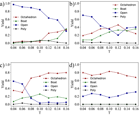
Figure S1: Yield as a function of temperature for 4 different patchy particle core sizes, a) 0.1, b) 0.2, c) 0.3, and d) 0.4. The black line represents the structures that have closed but are neither the boat or the octahedron. Results were averaged over 100 samples.

In Fig. S1 we show yield results for four different core sizes. We define the yield as the probability of forming a given shell. We divide the yield in four categories, the boat, the icosahedron, the open or misfolded shells, and the polymorph structures, which are structures that have closed but they are neither the octahedron or the boat. This can happen since the core is spherical and patches are point-like. Thus, if the core is too small different faces can cross each other and form non-physical bonds. We observe that the amount of non-physical structures becomes negligible around a core size of $0.2$. Nonetheless, at $0.2$ the number of incomplete nets is still quite large, since faces can still overlap easily. On the other hand, at core size of $0.4$ the boat structure can no longer form. Thus, we decided to fix the core size at $0.3$ (Fig. 2), since both structures can close and the probability of face overlap is negligible.

.3 SAT clauses

One can map the patchy particle design into a SAT problem by translating it into boolean variables and then imposing constraints such that the structures in Fig. 1 are formed.

The boolean variables can be divided into four categories. The first one is the color interaction variables, $x_{c_{i},c_{j}}^{int}$, where $c_{i}$ and $c_{j}$ are the color of particle $i$ and $j$ respectively. If a variable is true then colors $c_{i}$ and $c_{j}$ interact and can form a bond, otherwise they cannot. There are a total of $(N_{c})(N_{c}+1)/2$ of these variables. The second category is the patch coloring variable, $x_{p,s,c}^{pcol}$, where $p\in[1,N_{p}]$ refers to particle species, $s\in[1,V]$ to patch number and color $c\in[1,N_{c}]$. If a variable is true then particle specie $p$ has the patch number $s$ of color $c$. There are $N_{p}VN_{c}$ of these variables. Then the structure placement variables, $x_{l,p,o}^{L}$, where $l\in[1,L]$ refers the position of a particle in the structures, $p\in[1,N_{p}]$ to particle specie and orientation $o\in[1,R]$. If a variable is true then a particle of species $p$ occupies position $l$ in the structure according to orientation $o$. There are $N_{p}LR$ of these variables. Lastly, there is an auxiliary variable, $x_{l,s,c}^{A}$. If a variable is true then the particle in position $l$ is oriented such that the patch $s$ has a color $c$. There are $VLN_{c}$ such variables. The orientation mapping is given in Table I.

There are seven categories of clauses solved by SAT. The first guarantees that each color can only interact with only one other color:

$$C^{int}_{c_{i},c_{j},c_{k}}=\neg x_{c_{i},c_{j}}^{int}\vee\neg x_{c_{i},c_{k}}^{int}$$ (S1)

The second ensures that patch number $s$ of particle specie $p$ will have exactly one color only:

$$C^{pcol}_{p,s,c_{k},c_{l}}=\neg x_{p,s,c_{k}}^{pcol}\vee\neg x_{p,s,c_{l}}^{pcol}$$ (S2)

The third guarantees that position $l$ is occupied by exactly one particle specie with one orientation:

$$C^{L}_{l,p_{i},o_{i},p_{j},o_{j}}=\neg x_{l,p_{i},o_{i}}^{L}\vee\neg x_{l,p_{j},o_{j}}^{L}$$ (S3)

The fourth enforces that the neighboring positions $l_{i}$ and $l_{j}$ connected by the patches $s_{i}$ and $s_{j}$ have colors in those patches, $c_{i}$ and $c_{j}$, which interact:

$$C^{lint}_{l_{i},s_{i},l_{j},s_{j},c_{i},c_{j}}=\neg x_{l_{i},s_{i},c_{i}}^{A}\vee\neg x_{l_{j},s_{j},c_{j}}^{A}\vee x_{c_{i},c_{j}}^{int}$$ (S4)

The fifth ensures that for a position $l$ that is occupied by particle specie $p$ with orientation $o$, the patch $s$ has the right color attributed to it:

$$\begin{split}C^{LS}_{l,p,o,c,s}=&(\neg x_{l,p,o}^{L}\vee\neg x_{l,s,c}^{A}\vee x_{p,\phi_{o}(s),c}^{pcol})\\ &\wedge(\neg x_{l,p,o}^{L}\vee x_{l,s,c}^{A}\vee\neg x_{p,\phi_{o}(s),c}^{pcol})\end{split}$$ (S5)

The two last categories define multiple clauses each, the first enforces that all particle species are used, while the second enforces that all colors are used:

$$\forall p\in[1,N_{p}]:C_{p}^{allp.}=\underset{\forall l\in[1,L],o\in[1,R]}{\bigvee}x_{l,p,o}^{L}$$ (S6)

$$\forall c\in[1,N_{c}]:C_{c}^{allc.}=\underset{\forall p\in[1,N_{p}],s\in[1,V]}{\bigvee}x_{p,s,c}^{pcol}$$ (S7)

Orientation $o$	Mapping $\phi_{o}$
1	(1,2,3)
2	(3,1,2)
3	(2,3,1)

Table 1: Mapping of the orientation to the patch numbers

.4 Individual yields for $E_{r}$ and $T$

In Fig. 3 we show the order parameter histogram for different values of $E_{r}$. It is possible to observe that as $E_{r}$ increases, the octahedron becomes more probable for all temperature ranges explored.

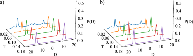
Figure S2: order parameter histograms as a function of temperature for 2 different values of $E_{r}$, a) 0.6, and b) 0.7. Results were averaged over 100 samples and 100 time-steps.

References

- Whitelam and Jack [2015] S. Whitelam and R. L. Jack, The Statistical Mechanics of Dynamic Pathways to Self-Assembly, Annual Review of Physical Chemistry 66, 143 (2015), arXiv:1407.2505 .
- Meng et al. [2010] G. Meng, N. Arkus, M. P. Brenner, and V. N. Manoharan, The free-energy landscape of clusters of attractive hard spheres, Science 327, 560 (2010), https://www.science.org/doi/pdf/10.1126/science.1181263 .
- Garmann et al. [2022] R. F. Garmann, A. M. Goldfain, C. R. Tanimoto, C. E. Beren, F. F. Vasquez, D. A. Villarreal, C. M. Knobler, W. M. Gelbart, and V. N. Manoharan, Single-particle studies of the effects of rna–protein interactions on the self-assembly of rna virus particles, Proceedings of the National Academy of Sciences 119, e2206292119 (2022), https://www.pnas.org/doi/pdf/10.1073/pnas.2206292119 .
- Pandey et al. [2011] S. Pandey, M. Ewing, A. Kunas, N. Nguyen, D. H. Gracias, and G. Menon, Algorithmic design of self-folding polyhedra, Proceedings of the National Academy of Sciences 108, 19885 (2011), https://www.pnas.org/doi/pdf/10.1073/pnas.1110857108 .
- Frenkel and Wales [2011] D. Frenkel and D. J. Wales, Designed to yield, Nature Materials 10, 410 (2011).
- Sartori and Leibler [2020] P. Sartori and S. Leibler, Lessons from equilibrium statistical physics regarding the assembly of protein complexes, Proceedings of the National Academy of Sciences 117, 114 (2020), https://www.pnas.org/doi/pdf/10.1073/pnas.1911028117 .
- Vo and Glotzer [2022] T. Vo and S. C. Glotzer, A theory of entropic bonding, Proceedings of the National Academy of Sciences 119, e2116414119 (2022).
- Dodd et al. [2018] P. M. Dodd, P. F. Damasceno, and S. C. Glotzer, Universal folding pathways of polyhedron nets, Proceedings of the National Academy of Sciences 115, E6690 (2018), https://www.pnas.org/doi/pdf/10.1073/pnas.1722681115 .
- Joshi et al. [2016] D. Joshi, D. Bargteil, A. Caciagli, J. Burelbach, Z. Xing, A. S. Nunes, D. E. P. Pinto, N. A. M. Araújo, J. Brujic, and E. Eiser, Kinetic control of the coverage of oil droplets by DNA-functionalized colloids, Science Advances 2, e1600881 (2016), arXiv:1603.05931 .
- Bupathy et al. [2022] A. Bupathy, D. Frenkel, and S. Sastry, Temperature protocols to guide selective self-assembly of competing structures, Proceedings of the National Academy of Sciences 119, e2119315119 (2022), https://www.pnas.org/doi/pdf/10.1073/pnas.2119315119 .
- Faber et al. [2018] J. A. Faber, A. F. Arrieta, and A. R. Studart, Bioinspired spring origami, Science 359, 1386 (2018), https://www.science.org/doi/pdf/10.1126/science.aap7753 .
- Kim et al. [2023] M. Kim, C. Lee, K. Jeon, J. Y. Lee, Y.-J. Kim, J. G. Lee, H. Kim, M. Cho, and D.-N. Kim, Harnessing a paper-folding mechanism for reconfigurable dna origami, Nature 619, 78 (2023).
- Geerts and Eiser [2010] N. Geerts and E. Eiser, Dna-functionalized colloids: Physical properties and applications, Soft Matter 6, 4647 (2010).
- Chen et al. [2022] K. Chen, F. Xu, Y. Hu, H. Yan, and L. Pan, Dna kirigami driven by polymerase-triggered strand displacement, Small 18, 2201478 (2022).
- Tang et al. [2023] Y. Tang, H. Liu, Q. Wang, X. Qi, L. Yu, P. Šulc, F. Zhang, H. Yan, and S. Jiang, Dna origami tessellations, Journal of the American Chemical Society 145, 13858 (2023), pMID: 37329284, https://doi.org/10.1021/jacs.3c03044 .
- Wintersinger et al. [2023] C. M. Wintersinger, D. Minev, A. Ershova, H. M. Sasaki, G. Gowri, J. F. Berengut, F. E. Corea-Dilbert, P. Yin, and W. M. Shih, Multi-micron crisscross structures grown from dna-origami slats, Nature Nanotechnology 18, 281 (2023).
- Sussman et al. [2015] D. M. Sussman, Y. Cho, T. Castle, X. Gong, E. Jung, S. Yang, and R. D. Kamien, Algorithmic lattice kirigami: A route to pluripotent materials, Proceedings of the National Academy of Sciences 112, 7449 (2015), https://www.pnas.org/doi/pdf/10.1073/pnas.1506048112 .
- Araújo et al. [2018] N. A. M. Araújo, R. A. da Costa, S. N. Dorogovtsev, and J. F. F. Mendes, Finding the optimal nets for self-folding kirigami, Phys. Rev. Lett. 120, 188001 (2018).
- Melo et al. [2020] H. P. M. Melo, C. S. Dias, and N. A. M. Araújo, Optimal number of faces for fast self-folding kirigami, Communications Physics 3, 154 (2020).
- Simões et al. [2021] T. S. A. N. Simões, H. P. M. Melo, and N. A. M. Araújo, Lattice model for self-folding at the microscale, The European Physical Journal E 44, 46 (2021).
- Azam et al. [2009] A. Azam, T. G. Leong, A. M. Zarafshar, and D. H. Gracias, Compactness determines the success of cube and octahedron self-assembly, PLOS ONE 4, 1 (2009).
- Russo et al. [2022] J. Russo, F. Romano, L. Kroc, F. Sciortino, L. Rovigatti, and P. Šulc, SAT-assembly: a new approach for designing self-assembling systems, Journal of Physics: Condensed Matter 34, 354002 (2022).
- Eén and Biere [2005] N. Eén and A. Biere, Effective preprocessing in SAT through variable and clause elimination, Lecture Notes in Computer Science 3569, 61 (2005).
- Chen et al. [2020] S. Chen, J. Chen, X. Zhang, Z.-Y. Li, and J. Li, Kirigami/origami: unfolding the new regime of advanced 3d microfabrication/nanofabrication with “folding”, Light: Science & Applications 9, 75 (2020).
- Jun et al. [2021] H. Jun, X. Wang, M. F. Parsons, W. P. Bricker, T. John, S. Li, S. Jackson, W. Chiu, and M. Bathe, Rapid prototyping of arbitrary 2D and 3D wireframe DNA origami, Nucleic Acids Research 49, 10265 (2021).
- Russo et al. [2009] J. Russo, P. Tartaglia, and F. Sciortino, Reversible gels of patchy particles: Role of the valence, The Journal of Chemical Physics 131, 014504 (2009), https://doi.org/10.1063/1.3153843 .
- Bohlin et al. [2023] J. Bohlin, A. J. Turberfield, A. A. Louis, and P. Šulc, Designing the self-assembly of arbitrary shapes using minimal complexity building blocks, ACS Nano 17, 5387 (2023), pMID: 36763807, https://doi.org/10.1021/acsnano.2c09677 .
- Pinto et al. [2023] D. E. P. Pinto, P. Šulc, F. Sciortino, and J. Russo, Design strategies for the self-assembly of polyhedral shells, Proceedings of the National Academy of Sciences 120, e2219458120 (2023), https://www.pnas.org/doi/pdf/10.1073/pnas.2219458120 .
- Tikhomirov et al. [2017] G. Tikhomirov, P. Petersen, and L. Qian, Fractal assembly of micrometre-scale dna origami arrays with arbitrary patterns, Nature 552, 67 (2017).
- Murugan et al. [2015] A. Murugan, Z. Zeravcic, M. P. Brenner, and S. Leibler, Multifarious assembly mixtures: Systems allowing retrieval of diverse stored structures, Proceedings of the National Academy of Sciences 112, 54 (2015).
- Fink and Ball [2001] T. M. Fink and R. C. Ball, How many conformations can a protein remember?, Physical review letters 87, 198103 (2001).
- Lowensohn et al. [2020] J. Lowensohn, A. Hensley, M. Perlow-Zelman, and W. B. Rogers, Self-assembly and crystallization of dna-coated colloids via linker-encoded interactions, Langmuir 36, 7100 (2020).