Towards Unified Deep Image Deraining:
A Survey and A New Benchmark

Abstract

Recent years have witnessed significant advances in image deraining due to the kinds of effective image priors and deep learning models. As each deraining approach has individual settings (e.g., training and test datasets, evaluation criteria), how to fairly evaluate existing approaches comprehensively is not a trivial task. Although existing surveys aim to review of image deraining approaches comprehensively, few of them focus on providing unify evaluation settings to examine the deraining capability and practicality evaluation. In this paper, we provide a comprehensive review of existing image deraining method and provide a unify evaluation setting to evaluate the performance of image deraining methods. We construct a new high-quality benchmark named HQ-RAIN to further conduct extensive evaluation, consisting of 5,000 paired high-resolution synthetic images with higher harmony and realism. We also discuss the existing challenges and highlight several future research opportunities worth exploring. To facilitate the reproduction and tracking of the latest deraining technologies for general users, we build an online platform to provide the off-the-shelf toolkit, involving the large-scale performance evaluation. This online platform and the proposed new benchmark are publicly available and will be regularly updated at http://www.deraining.tech/.

1 Introduction

Rain is a challenging adverse weather condition which always obstructs or deforms the image background. It consequently degrades the visual quality of images and impairs the performance of outdoor vision-based systems, including video surveillance [1], autonomous driving [2] and person identification [3], etc. Single image deraining, also known as rain removal, aims to recover the rain-free image from the observed rainy one. A large number of deraining methods and benchmark datasets have been proposed in recent years with demonstrated success. Since this topic booms with the deep learning techniques [4, 5, 6, 7], it is significant to timely and comprehensively evaluate the state-of-the-art approaches to demonstrate their strength and weakness, thus facilitating the future development of this research field for more robust algorithms.

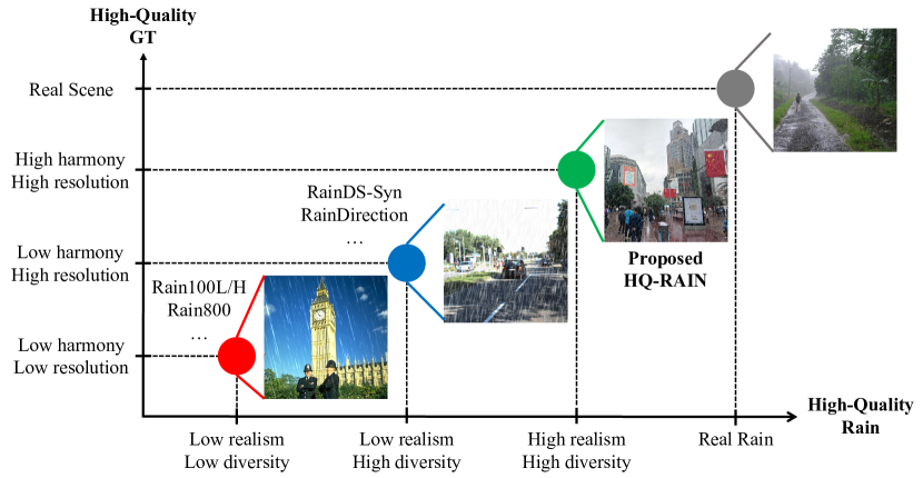
(a) Analysis of Benchmark Characteristic

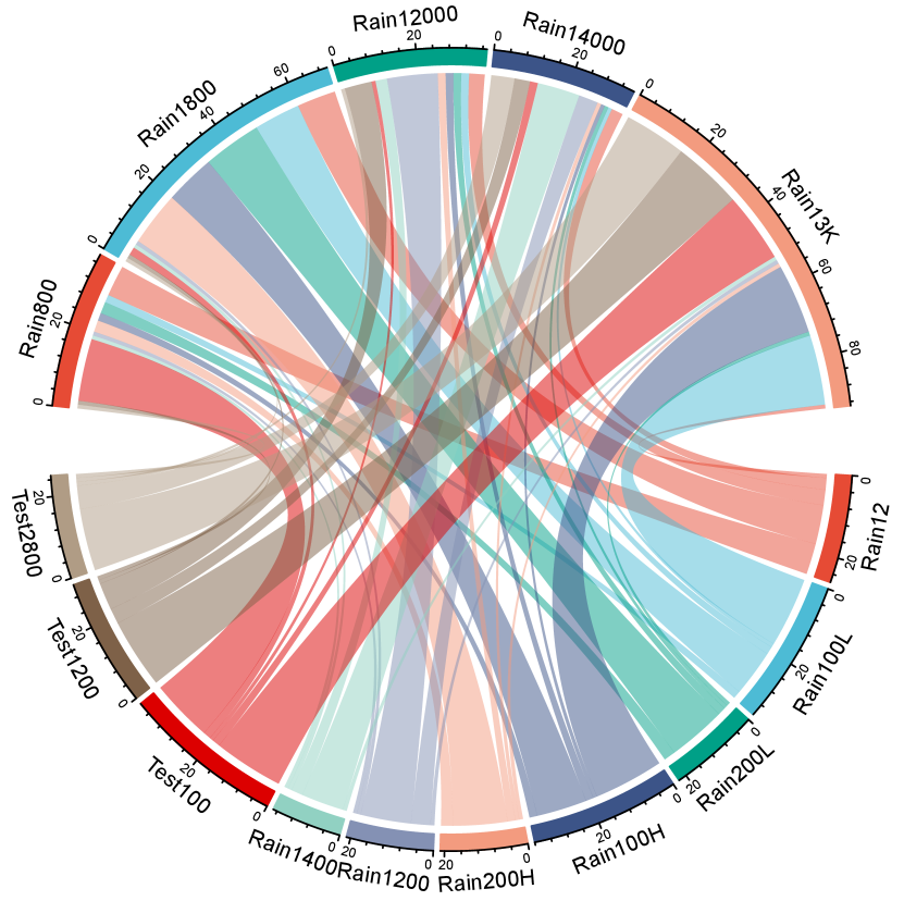
(b) Analysis of Benchmark Usage

Figure 1: Analysis of commonly used synthetic benchmark characteristic and usage based on over a hundred literatures about image deraining. (a) Our proposed new benchmark narrows the domain gap between real rainy images, due to its properties of high-quality rain with higher realism and diversity, and high-quality GT with higher harmony and resolution. (b) Statistics on the usage relationship between training and test datasets in their experiments with existing methods. The upper semicircle means training datasets, and the lower semicircle means testing datasets.

To facilitate the performance comparison and analysis of existing methods, it is indispensable to collect a representative benchmark dataset. There exist several classical synthetic datasets for single image deraining task, such as the Rain100L [8], Rain100H [8], and Rain800 [5]. Although these synthetic datasets are prevalent in current studies [9, 10, 11, 12, 13, 14], most approaches randomly add rain effects to any clear backgrounds to build the synthetic paired data, which inevitably leads to inadequate realism and harmony, especially in the sky region (see Figure 1(a)). As a result, there is a large domain gap between synthetic and real data, which limits the ability of training better deep deraining models. Recently, significant efforts have been made to solve real-world image deraining, where the large-scale datasets are proposed, e.g, SPA-Data [15] and GT-RAIN [16]. Unfortunately, these real datasets still have several shortcomings, including low resolution, spatial misalignment, limited rain appearances and background variation [17]. In fact, obtaining strictly aligned rainy and clear image pairs in complex rainy environments is time-consuming and laborious. Returning to the problem itself, it is urgent and necessary to establish a high-quality benchmark and pave the way for future research in this field.

Despite lots of efforts have been made on existing benchmarks[4, 5, 6, 17, 7], there still exist several potential challenges. According to statistics in Figure 1(b), existing methods usually use individual evaluation settings to evaluate the deraining performance. The evaluations based on different settings do not fully reflect performance to some extent. On one side, multiple training sets are trained in a mixed way, and a pretrained model is obtained to evaluate different testing sets. The typical mixed training based methods include MSPFN [18], MPRNet [19], Restormer [20]. On the other side, each training set is trained independently, and multiple pretrained models are obtained to evaluate the corresponding testing sets. The typical independent training based methods include SPDNet [12], IDT [11], DRSformer [9]. Under the setting of independent training, the usage relationships between training data and testing data are also quite diverse, especially for Rain100L/H and its new version, Rain200L/H [8]. As a result, this makes it difficult to make comparisons among the reported quantitative results. In addition, the validation metrics of the evaluated deraining algorithms are not the same, such as calculating PSNR and SSIM metric [21] in different channels (RGB or Y), and converting YCbCr space by MATLAB or OpenCV tool in different ways. This naturally leads to incomparable and sometimes contradictory quantitative results reported in their literature. Hence, it is of importance to integrate them in a unified track for evaluation on a common criteria.

Towards these goals, we first establish the latest development milestone of single image deraining field, especially with the increasing number of solutions in recent years. Note that this paper only focuses on image deraining, excluding video deraining. Based on this survey, we intend to summarize two tracks (i.e., mixed training and independent training) to report the performance of existing representative methods within the same evaluation criteria. It can provide a guideline on fair and reasonable comparisons of different methods in future work for researchers, especially for beginners who are new to this filed. We suggest that researchers can first try to categorize their methods into the corresponding track, and then pay special attention to evaluating and comparing previous methods that belong to the same track. Furthermore, we also construct a new high-quality image deraining benchmark, called HQ-RAIN, to further facilitate the performance comparison. To the best of our knowledge, this is the first attempt to improve the realism and harmony of synthetic rainy images, with the aim of reducing the domain gap between the synthetic and real data. Inspired by image harmonization [22], we can treat a real rainy image as harmonized image, and further generate a synthetic rainy dataset by background collection, rain streaks synthesis and image blending, making it compatible with the background area in the synthetic image. In addition to reviewing and analyzing the existing methods, we also develop a unified online platform to facilitate the performance evaluation. To keep pace with the fast development, this platform releases a public repository to provide an up-to-date record of recent advancements, which can be served as a reference point for new researchers. The online platform and the proposed new benchmark can be found at http://www.deraining.tech.

1.1 Our Contributions

The contribution of this paper are mainly three-fold. (1) We present a systematic and comprehensive review of recent advancements in single image deraining field. (2) We construct a new high-quality image deraining banchmark (called HQ-RAIN) to inspire further researches for more robust algorithms. (3) We provide an online platform to offer a fair and unified performance evaluation for deep image deraining methods.

1.2 Relations with Other Surveys

Despite the fact that deep learning has dominated image deraining research, a timely and thorough survey on the latest technologies is lacking. There are two early surveys of image deraining [4, 6] that mainly review prior-based and CNN-based methods. In comparison to recent survey [7] that reviews current methods from different perspectives, this paper seeks to provide much more than a summary of recent research progress. Although these surveys have provided comprehensive analyses of existing datasets, they still overlook two key factors when evaluting existing algorithms: synthetic dataset quality and common evaluation criteria. To the best of our knowledge, these two issues have not been well addressed in the literatures of image deraining. Our survey will fill the gap in this research.

1.3 Organization

The rest of this paper is structured as follows. In Section 2, we present the problem formulations of some common rainy image models. Section 3 provides a systematic review of representative image deraining methods. Section 4 introduces our proposed new benchmark. In Section 5, we conduct extensive performance evaluations and analyses for representative methods. Section 6 discusses the open challenges and new perspectives for future studies. Finally, the concluding remarks will be drawn in Section 7.

2 Problem Formulation

In this section, we review several representative rain models proposed in the existing methods. These different rain models can be used to simulate various types of rain degradation. It should be noted that all these models are heuristic, as they are only rough approximations of the real world.

Linear Superposition Model (LSM).

The most of the existing methods adpot simple and common rain model, i.e., linear superposition model (LSM), to achieve the separation of undesired rain streaks and latent clear background. The rainy image $\mathbf{R}$ degraded by rain streaks is formulated as:

$$\mathbf{R}=\mathbf{B}+\mathbf{S},$$ (1)

where $\mathbf{B}$ and $\mathbf{S}$ represent the rain-free background layer and the rain streak layer, respectively. For convenience, we use the uniform mathematical symbols in the following.

Screen Blend Model (SBM).

Different from the LSM, Luo et al. [23] formulate a non-linear composite model, i.e., screen blend model (SBM), for modeling rainy images. It considers that the rain streak layer and background layer may affect the apperance of each other, which can be expressed as:

$$\mathbf{R}=\mathbf{B}+\mathbf{S}-\mathbf{B}\odot\mathbf{S},$$ (2)

where $\odot$ denotes the element-wise multiplication operator. According to [23], these rainy images rendered by the SBM tend to look more realistic than those by the LSM.

Heavy Rain Model (HRM).

In the case of heavy rain, the accumulation of distant rain streaks and water particles in the atmosphere leads to the rain veiling effect. This visual effect of rain accumulation produces a mist (or haze)-like phenomenon in the image background [8]. Based on the joint observation of the rain streak model and the atmospheric scattering model [24], the formulation of this heavy rain model (HRM) is defined as:

$$\mathbf{R}=\left(\mathbf{B}+\sum_{i=1}^{n}\mathbf{S}_{i}\right)\odot\mathbf{T}+(1-\mathbf{T})\odot\mathbf{A},$$ (3)

where $\mathbf{T}$ and $\mathbf{A}$ refers to the transmisson map and the global atmospheric light, respectively. Each $\mathbf{S}_{i}$ is termed as the rain streak layer with the same direction. Here, $i$ is the number of the rain streak layers, and its maximum value is $n$.

Depth-guided Rain Model (DRM).

Hu et al. [25] formulate a rain imaging model based on the visual effects of rain in relation to scene depth information. The visibility of distant objects varies with depth from the camera, and fog visibly obscures those distant objects more than rain streaks do. The mathematical model of the depth-guided rain model (DRM) is introducted as:

$$\mathbf{R}=\left(1-\mathbf{S}-\mathbf{F}\right)\odot\mathbf{B}+\mathbf{S}+\mathbf{F}\odot\mathbf{A},$$ (4)

where $\mathbf{F}\in[0,1]$ represents the fog layer. $\mathbf{F}$ is further written as $\mathbf{F}=1-e^{-\beta d(x)}$, where $\beta$ determines the thickness of fog, and $d(x)$ denotes the scene depth.

Transmission Medium Model (TMM).

Based on the observation that rain streaks and vapors are entangled with each other, Wang et al. [26] remodel rain imaging by formulating both rain streaks and vapors as transmission medium, which is formulated as:

$$\mathbf{R}=\left(\mathbf{T}_{\mathbf{s}}+\mathbf{T}_{\mathbf{v}}\right)\odot\mathbf{B}+\left[1-\left(\mathbf{T}_{\mathbf{s}}+\mathbf{T}_{\mathbf{v}}\right)\right]\odot\mathbf{A},$$ (5)

where $\mathbf{T}_{\mathbf{s}}$ and $\mathbf{T}_{\mathbf{v}}$ represent the transmission map of rain streaks and vapors, respectively.

Raindrop Mask Model (RMM).

The clear background image may be obscured or blurred by persistent raindrops that cling to camera lenses or window glasses as they fall and flow [27]. Qian et al. [28] formulate a raindrop degraded image as the result of combining the raindrop effect and the background image:

$$\mathbf{R}=(1-\mathbf{M})\odot\mathbf{B}+\mathbf{D},$$ (6)

where $\mathbf{D}$ denotes the obstruction or blurry effect brought by the raindrops. $\mathbf{M}$ is the binary mask. If $\mathbf{M}(x)=1$, the pixel $x$ in the mask belongs to the raindrop region, otherwise it is a part of the background image.

Mixture of Rain Model (MRM).

During outdoor image capturing, rain streaks and raindrops may co-occur. The lighting conditions that have a significant impact on the transparency of the raindrops during image capture may alter as a result of rain streaks. As a result, removing rain streaks and raindrops cannot simply be construed as a rain streak removal and a raindrop removal combined. The mixture of rain model (MRM) [29] can be modeled as:

$$\mathbf{R}=(\mathbf{1}-\mathbf{M})\odot(\mathbf{B}+\mathbf{S})+\alpha\mathbf{D},$$ (7)

where $\alpha$ indicates the atmospheric lighting coefficient.

3 Technical Development Review

In this section, we first provide a latest milestone of single image deraining in Table I. Then, we analyze the technical characteristics of the deep learning-based methods from five main perspectives of the learning strategies, network structures, loss functions, experimental datasets, and evaluation metrics. In what follows, we select representative methods based on the following principles: publishing in well-known journals (e.g., TPAMI, IJCV) and conferences (e.g., CVPR, ICCV), providing the official codes to ensure credibility, preferring works with more citations and Github stars.

TABLE I: Summarization of representative single image deraining methods. “SL”, “SSL” and “UL” stand for supervised/semi-supervised/unsupervised learning-based methods. “CE”, “Adv”, “KL”, “TV”, “Contra” and “QS” denote cross entropy loss, adversarial loss, Kullback Leibler loss, total variation loss, contrastive loss and quasi-sparsity loss, respectively. “self-selected” denotes images selected by the author rather than common datasets. “P”, “R”, “F” and “U” represent parameter, run-time, FLOPs and user study, respectively. “-” means this item is not available or not indicated in their paper.

	Method	Category	Learning	Network Structure	Loss Function	Experimental Dataset	Evaluation Metric	Platform	Venue
	Image Decomposition [30]	Prior	-	-	-	self-selected	VIF #R	MATLAB	TIP
	DSC [23]	Prior	-	-	-	self-selected	PSNR SSIM	MATLAB	ICCV
	GMM [31]	Prior	-	-	-	Rain12	SSIM	MATLAB	CVPR
2017	JBO [32]	Prior	-	-	-	self-selected	PSNR SSIM	MATLAB	ICCV
	JCAS [33]	Prior	-	-	-	Rain12	SSIM	MATLAB	ICCV
	DerainNet [34]	CNN	SL	three layers	$L_{2}$	Rain12	SSIM BIQE #R	MATLAB	TIP
	DDN [35]	CNN	SL	residual network	$L_{2}$	Rain14000	SSIM #R	Caffe	CVPR
	JORDER [8]	CNN	SL	multi-task network	$L_{2}$+CE	Rain100L/H Rain12	PSNR SSIM #R	Caffe	CVPR
2018	DID-MDN [36]	CNN	SL	multi-stream network	$L_{2}$+CE	DID-Data	PSNR SSIM #R	PyTorch	CVPR
	AttentGAN [28]	GAN	SL	recurrent network	$L_{2}$+Adv	RainDrop	PSNR SSIM	PyTorch	CVPR
	DualCNN [37]	CNN	SL	multi-branch network	$L_{2}$	Rain800	PSNR	PyTorch	CVPR
	RESCAN [38]	CNN	SL	recurrent network	$L_{2}$	Rain100H Rain800	PSNR SSIM	PyTorch	ECCV
	NLEDN [39]	CNN	SL	non-local network	$L_{1}$	Rain100L/H DNN-Data DID-Data	PSNR SSIM	PyTorch	ACM MM
	ResGuideNet [40]	CNN	SL	residual network	$L_{2}$+SSIM	Rain100/H Rain12	PSNR SSIM #P #R	TensorFlow	ACM MM
2019	GCANet [41]	CNN	SL	gated network	$L_{2}$	DID-Data	PSNR SSIM	PyTorch	WACV
	PReNet [42]	CNN	SL	recursive network	SSIM	Rain100/H Rain12	PSNR SSIM #R	PyTorch	CVPR
	DAF-Net [25]	CNN	SL	residual network	$L_{2}$	RainCityscapes Rain100H	PSNR SSIM	Caffe	CVPR
	HeavyRainRemoval [43]	GAN	SL	multi-stage network	$L_{1}$+$L_{2}$+Adv	NYU-Rain Outdoor-Rain	PSNR SSIM	PyTorch	CVPR
	SPANet [15]	CNN	SL	multi-stage network	$L_{1}$+$L_{2}$+Adv	SPA-Data DID-Data	PSNR SSIM	PyTorch	CVPR
	UMRL [44]	CNN	SL	multi-scale network	$L_{1}$	DID-Data Rain800	PSNR SSIM	PyTorch	CVPR
	SIRR [45]	CNN	SSL	two subnetworks	$L_{2}$+KL+TV	DDN-SIRR	PSNR SSIM	TensorFlow	CVPR
	RaindropAttention [46]	CNN	SL	U-Net like network	$L_{1}$	RainDrop	PSNR SSIM	TensorFlow	ICCV
	ERL-Net [47]	CNN	SL	U-Net like network	$L_{1}$	DDN-Data DID-Data	PSNR SSIM	TensorFlow	ICCV
	ID-CGAN [48]	GAN	SL	two subnetworks	$L_{2}$+Adv	Rain800	PSNR SSIM UQI VIF #R	PyTorch	TCSVT
	DTDN [49]	GAN	SL	multi-task network	$L_{2}$+Adv	DID-Data	PSNR SSIM UQI	Keras	ACM MM
	GraNet [50]	CNN	SL	multi-stage network	$L_{1}$	Rain100L/H Rain12	PSNR SSIM	PyTorch	ACM MM
	ReHEN [51]	CNN	SL	multi-stage network	$L_{2}$+SSIM	Rain100L/H Rain800 DNN-Data DID-Data	PSNR SSIM	TensorFlow	ACM MM
	LPNet [52]	CNN	SL	pyramid network	$L_{1}$+SSIM	Rain100L/H Rain12	PSNR SSIM #P #R	TensorFlow	TNNLS
	JORDER-E [53]	CNN	SL	multi-task network	$L_{1}$+$L_{2}$	Rain100L/H Rain800 Rain12	PSNR SSIM #R	Caffe	TPAMI
	RR-GAN [54]	GAN	UL	multi-scale network	$L_{2}$+Adv	Rain800	PSNR SSIM	PyTorch	AAAI
	UD-GAN [55]	GAN	UL	multi-task network	$L_{1}$+Adv	Rain100L/H Rain800 Rain12	PSNR SSIM #U #R	PyTorch	ICIP
	DualResidualNetwork [56]	CNN	SL	residual network	$L_{1}$+SSIM	DDN-Data DID-Data	PSNR SSIM	PyTorch	CVPR
2020	MSPFN [18]	CNN	SL	multi-scale network	$L_{1}$	Rain13K	PSNR SSIM FSIM NIQE SSEQ	TensorFlow	CVPR
	DRD-Net [14]	CNN	SL	two subnetworks	$L_{2}$	Rain200/H Rain800	PSNR SSIM #R	TensorFlow	CVPR
	RCDNet [57]	CNN	SL	multi-stage network	$L_{2}$	Rain100L/H Rain12 DDN-Data SPA-Data	PSNR SSIM	PyTorch	CVPR
	Syn2Real [58]	CNN	SSL	U-Net like network	$L_{1}$+$L_{2}$	DDN-SIRR	PSNR SSIM NIQE BRISQUE	PyTorch	CVPR
	All-in-One [59]	GAN	SL	architectural search	$L_{2}$	Outdoor-Rain Raindrop	PSNR SSIM	-	CVPR
	CVID [60]	CNN	SL	auto-encoder network	$L_{2}$+KL	Rain100L/H DNN-Data DID-Data	PSNR SSIM NIQE #R	TensorFlow	TIP
	Physics GAM [61]	GAN	SL	two subnetworks	$L_{1}$+Adv	self-selected	PSNR SSIM	PyTorch	TPAMI
	FBL [62]	CNN	SL	recurrent network	$L_{1}$	Rain100/H Rain800	PSNR SSIM	PyTorch	AAAI
	PRRNet [63]	CNN	SL	multi-stage network	$L_{1}$+$L_{2}$+CE	RainCityscapes RainKITTI2012/2015	PSNR SSIM	PyTorch	ECCV
	SNet [26]	CNN	SL	multi-branch network	$L_{1}$+$L_{2}$	self-selected	PSNR SSIM FID #R	PyTorch	ECCV
	DCSFN [64]	CNN	SL	multi-scale network	SSIM	Rain100L Rain100H DID-Data	PSNR SSIM NIQE	PyTorch	ACM MM
	JDNet [65]	CNN	SL	non-local network	SSIM	Rain100L Rain100H Rain12	PSNR SSIM	PyTorch	ACM MM
2021	DualGCN [13]	CNN	SL	graph network	$L_{2}$	Rain200L/H Rain12 DID-Data DDN-Data SPA-Data	PSNR SSIM	TensorFlow	AAAI
	DerainCycleGAN [66]	GAN	UL	CycleGAN	$L_{1}$+$L_{2}$+Adv	Rain100L Rain12 Rain800 SPA-Data	PSNR SSIM	PyTorch	TIP
	IPT [67]	Transformer	SL	multi-task network	$L_{1}$+Contra	Rain100L	PSNR SSIM	PyTorch	CVPR
	MPRNet [19]	CNN	SL	multi-stage network	$L_{1}$	Rain13K	PSNR SSIM #P #R	PyTorch	CVPR
	CCN [29]	CNN	SL	architectural search	$L_{1}$+SSIM	RainDS Rain200L/H RainDrop	PSNR SSIM	PyTorch	CVPR
	MOSS [68]	CNN	SSL	U-Net like network	$L_{1}$+TV	DDN-SIRR	PSNR SSIM #R	PyTorch	CVPR
	RLNet [69]	CNN	SL	feedback network	$L_{1}$+$L_{2}$+SSIM	Rain100L Rain200H Rain800 DID-Data	PSNR SSIM NIQE #F #R	PyTorch	CVPR
	VRGNet [70]	GAN	SL	four subnetworks	Adv+KL	Rain100L/H DDN-Data	PSNR SSIM #U	PyTorch	CVPR
	JRGR [71]	GAN	SL	CycleGAN	$L_{1}$+$L_{2}$+Adv	RainCityscape	PSNR SSIM	PyTorch	CVPR
	RIC-Net [72]	GAN	SL	U-Net like network	$L_{1}$+$L_{2}$+Adv	RainLevel5 Rain800 Rain200H DID-Data SPA-Data	PSNR SSIM	PyTorch	CVPR
	QSMD [73]	CNN	SL	multi-scale network	$L_{1}$+$L_{2}$+QS	self-selected	PSNR SSIM #R	PyTorch	CVPR
	SPDNet [12]	CNN	SL	recursive network	$L_{2}$	Rain200L/H Rain800 DID-Data SPA-Data	PSNR SSIM #P #R	PyTorch	ICCV
	UDRDR [74]	CNN	SSL	three subnetworks	$L_{2}$+TV	Rain100L/H DID-Data RainDirection	PSNR SSIM NIQE #P #R	PyTorch	ICCV
	SPAIR [75]	CNN	SL	U-Net like network	$L_{1}$	Rain13K	PSNR SSIM	PyTorch	ICCV
	UDGNet [76]	CNN	UL	multi-task network	Adv+TV	RainCityscapes DDN-Data	PSNR SSIM NIQE #U #R	PyTorch	ACM MM
	EfficientDeRain [77]	CNN	SL	U-Net like network	$L_{1}$+SSIM	Rain100H DDN-Data SPA-Data RainDrop	PSNR SSIM #R	PyTorch	AAAI
	SWAED [78]	CNN	SL	U-Net like network	$L_{1}$	Rain100L/H Rain12 DDN-Data DID-Data	PSNR SSIM #R #F	PyTorch	IJCV
2022	DCD-GAN [79]	GAN	UL	CycleGAN	$L_{1}$+$L_{2}$+Adv	Rain800 DID-Data DDN-Data SPA-Data	PSNR SSIM NIQE BRISQUE	PyTorch	CVPR
	NLCL [80]	GAN	UL	two subnetworks	$L_{2}$+Contra	RainCityscapes SPA-Data	PSNR SSIM NIQE #P #R	PyTorch	CVPR
	Restormer [20]	Transformer	SL	U-Net like network	$L_{1}$	Rain13K	PSNR SSIM	PyTorch	CVPR
	Uformer [81]	Transformer	SL	U-Net like network	Charbonnier	SPA-Data	PSNR SSIM	PyTorch	CVPR
	DGUNet [82]	CNN	SL	multi-stage network	$L_{2}$	Rain13K	PSNR SSIM	PyTorch	CVPR
	MAXIM [83]	Transformer	SL	multi-stage network	$L_{1}$+Charbonnier	Rain13K	PSNR SSIM	PyTorch	CVPR
	AirNet [84]	CNN	SL	two subnetworks	$L_{1}$+Contra	Rain100L	PSNR SSIM	PyTorch	CVPR
	TransWeather [85]	Transformer	SL	recurrent network	$L_{1}$+$L_{2}$	Outdoor-Rain Raindrop	PSNR SSIM	PyTorch	CVPR
	SEIDNet [86]	CNN	SL	multi-branch network	$L_{2}$+SSIM	Rain13K DDN-Data SPA-Data	PSNR SSIM	PyTorch	NeurIPS
	ELF [87]	Transformer	SL	two subnetworks	Charbonnier	Rain13K	PSNR SSIM FSIM NIQE SSEQ #P #R #F	PyTorch	ACM MM
	IDT [11]	Transformer	SL	U-Net like network	SSIM	Rain200L/H DID-Data DDN-Data SPA-Data RainDS	PSNR SSIM #P #R #F	PyTorch	TPAMI
2023	HCT-FFN [88]	Transformer	SL	multi-stage network	$L_{2}$+SSIM	Rain100L/H Rain12 RainDS	PSNR SSIM NIQE BRISQUE	PyTorch	AAAI
	HCN [10]	CNN	SL	U-Net like network	$L_{1}$	Rain200L/H Rain12 DID-Data DDN-Data SPA-Data	PSNR SSIM	PyTorch	TPAMI
	WeatherDiffusion [89]	Diffusion	SL	U-Net like network	$L_{1}$	Outdoor-Rain Raindrop	PSNR SSIM NIQE	PyTorch	TPAMI
	DRSformer [9]	Transformer	SL	U-Net like network	$L_{1}$	Rain200L/H DID-Data DDN-Data SPA-Data	PSNR SSIM NIQE BRISQUE	PyTorch	CVPR
	SmartAssign [90]	CNN	SL	multi-task network	$L_{2}$+QS+Contra	DID-Data	PSNR SSIM	-	CVPR

3.1 Method Categories

Based on the problem formulations, image deraining methods can be categorized into model-based methods and data-driven methods [4, 6]. Early model-based approaches [91, 92, 93, 94, 95, 96] usually formulate the image deraining as a filtering problem and restore the rain-free image by kinds of filters. Although rain streaks can be removed, some important strictures are also removed during the filtering process. As image deraining is ill-posed, lots of model-based approaches develops kinds of image priors based on the statistical properties of rain streaks and clear images, including image decomposition [30], low-rank representation [97], discriminative sparse coding [23], and Gaussian mixture model [31], etc. Although better results have been achieved, these approaches cannot handle complex and varying rainy scenes because the hand-crafted rain models used these approaches do not hold. In addition, most algorithms [33, 32] still need time-consuming iterative computations due to the complexity of the optimization procedure.

Data-driven methods are able to learn models to better describe the properties of rain streaks and clear images. As one of the representative data-driven approach, image deraining based on deep learning approaches have achieved significant performance. Since the representative methods [34, 35, 8] have shown that using deep learning help rain removal, lot of approaches based on the convolutional neural networks (CNNs) [6, 34, 35, 36, 53, 18] have been developed to solve image deraining and achieve decent performance in kinds of image deraining benchmarks [4, 5, 6, 17]. To restore realistic images, lots of approaches employ generative adversarial networks (GANs) [98] to solve image deraining. With guidance of the adversarial learning strategy, the GAN-based methods [28, 48, 43, 61] are able to restore clear images with better perception quality.

However, as the basic operation in CNNs or GANs, the convolution operation is spatial invariant and has limited receptive field, which cannot model the spatial variant property and global structures of clear images well. To solve this problem, Transformers [99] have been applied to image deraining and achieve significant advancements as they can model the non-local information for better image reconstruction. Motivated by the success of recent diffusion model [100] in generating high-quality images, diffusion-based approaches [89] achieve promising results in kinds of image restoration problems, which may facilitate the image deraining problem.

In the following, we will briefly review the CNN-based, GAN-based, and Transformer-based representative deraining methods in details.

3.2 Learning Strategies

Along this research line, we categorize existing deep image deraining methods into supervised learning, unsupervised learning and semi-supervised learning. Based on the statistic analysis in Table I, supervised learning (86.2%) is the most widely used approach. There are emerging approaches starting in 2019 that make use of unsupervised learning (8.3%) and semi-supervised learning (5.5%). Next, we review some representative methods of each strategy.

Supervised Learning.

The classic deep learning-based image deraining baseline DerainNet [34] adopts a simple CNN to learn the nonlinear mapping function from paired clear and rainy images. Later, diverse network structures and designs have been extensively utilized to further enhance the ability of end-to-end learning, such as multi-scale fusion [64, 65] and multi-stage progressive [18, 19]. To better represent the rain distribution, several studies take rain characteristics such as rain density [36], location [8, 53], depth [25], sparsity [73], non-local [39], veiling effect [43, 26] into account. Recently, Transformers-based models have achieved significant performance in single image deraining due to their ability to model non-local information required for accurate image reconstruction. Xiao et al. [11] designed an image deraining Transformer (IDT) with spatial-based and complementary window-based Transformer modules. Very recently, Chen et al. [9] developed a Sparse Transformer (DRSformer) to achieve state-of-the-art (SOTA) performance in the category of supervised learning methods. Although impressive performance has been attained, these fully-supervised approaches require paired synthetic data, which poorly mimics the degradation that occurs in the real world. To this end, the semi-supervised and unsupervised learning have been proposed for image deraining [79, 101].

Unsupervised Learning.

To alleviate the pressure of collecting large-scale paired training data, unsupervised learning has been proposed for image deraining. In fact, learning a deep deraining network from unpaired data is more challenging compared to fully-supervised models. Zhu et al. [54] first proposed an end-to-end CycleGAN-based deraining model, RainRemoval-GAN (RR-GAN) without using paired training data. Jin et al. [55] presented an unsupervised deraining generative adversarial network (UD-GAN) by introducing self-supervised constraints from the intrinsic statistics of unpaired rainy and clear images. Another CycleGAN-based deraining network, termed as DerainCycleGAN [66], was designed using an unsupervised rain attentive detector. By modelling of the structure discrepancy between the clear image and rain distribution, Yu et al. [76] developed an unsupervised directional gradient based optimization model (UDGNet) for real rain streaks removal. Recently, Chen et al. [79] leveraged dual contrastive learning to encourage the model to explore the mutual features of rainy images and clean ones in the deep feature space, where the features from the unpaired clear exemplars can facilitate rain removal. Likewise, Ye et al. [80] incorporated non-local self-similarity into contrastive learning to further improve unsupervised image deraining performance.

Semi-supervised Learning.

Semi-supervised learning has recently been offered as a way to combine the advantages of supervised learning and unsupervised learning. Wei et al. [45] proposed the first semi-supervised image deraining (SSIR) framework, treating rain removal as domain adaption problem. The work of Syn2Real [58] was a Gaussian process based semi-supervised image deraining method by jointly modeling the labeled and unlabeled latent space. Huang et al. [68] presented a memory-oriented semi-supervised (MOSS) framework to adaptively record various appearances of rain degradations. In [74], the semi-supervised learning and knowledge distillation components were combined to formulate a rain direction regularizer, which can preserve the sharpness and structures of the rain maps. For unsupervised/semi-supervised rain removal, continued research in this direction is highly encouraged.

3.3 Network Architectures

Significant progress has been made due to the development of kinds of network architectures in image deraining. Next, we review the representative network designs in this field.

CNN-based Network Design.

Eigen et al. [102] designed the first CNN-based method by constructing a three-layer CNN that learns the mapping between corrupted image patches and their corresponding clean counterparts. Inspired by the deep residual network (ResNet) [103], Fu et al. [35] utilized the ResNet structure to integrate the high-frequency detail layer content of an image and perform regression on the negative residual rain information. Yang et al. [8] proposed a multi-task deep learning architecture that initially detects rain regions, which inherently provides supplementary information for the task of rain removal. To better characterize rain streaks of varying scales and shapes, a multi-stream densely connected framework was designed by [36], consisting of two main branches: rain-density classification and rain streak removal. Due to the overlapping nature of rain streak layers, removing rain in a single stage is challenging. Thus, Li et al. [38] decomposed the rain removal into multiple stages by introducing the recurrent neural network to retain useful information from previous stages and facilitate rain removal in subsequent stages. By formulating a rain imaging model based on the visual effects of rain in relation to scene depth information, Hu et al. further [25] proposed the depth-guided attention network to remove rain streaks and fog. Instead of deeper and complex networks, Ren et al. [42] discovered that a simple combination of ResNet with multi-stage recursion yields favorable deraining performance. Considering the role of spatial attention is to selectively focus on specific regions or locations in an image, Wang et al. [15] presented a spatial attention network designed to learn discriminative rain information in a local-to-global manner. Yasarla et al. [44] incorporated uncertainty-guided learning into the network to learn the residual maps and corresponding confidence maps at various scales. These maps are subsequently propagated back to guide the network in subsequent layers. By incorporating the Gaussian-Laplacian image pyramid decomposition technique, Fu et al. [52] proposed a lightweight pyramid network to simplify the learning problem. Inspired by the success of multi-scale strategies in vision tasks, Jiang et al. [18] proposed a multi-scale progressive fusion network that better characterizes rain streaks across multiple scales through the use of image pyramid representation. Wang et al. [57] proposed a rain convolutional dictionary network that leverages the inherent dictionary learning mechanism to accurately encode rain shapes. Deng et al. [14] constructed a two-branch parallel network consisting of a detail repair sub-network and a rain residual sub-network based on squeeze-and-excitation mechanism. To better compute channel-wise correlation and spatial-wise coherence, Fu et al. [13, 104] introduced a dual graph convolutional architecture to help image restoration and facilitate rain removal. Under the iterative guidance of the residue channel prior, Yi et al. [12] proposed a structure preserving deraining architecture to reconstruct high-quality rain-free images. Drawing on the concept of closed-loop control, Li et al. [69] designed a robust representation learning network structure by incorporating feedback mechanism into the CNN. Recently, Fu et al. [10] developed a patch-wise hypergraph convolutional network architecture to help the model to explore non-local content of the images.

GAN-based Network Design.

Driven by GAN in the image generation task [98], Qian et al. [28] incorporated a GAN-based architecture, where the generative network employs an attentive-recurrent network to generate an attention map. This attention map, along with the input image, is then utilized in a contextual autoencoder to generate a rain-free result. Afterwards, Zhang et al. [48] proposed a conditional GAN-based architecture with a densely-connected generator and a multi-scale discriminator. To achieve heavy rain image restoration, the method of Li et al. [43] consists of a two-stage network architecture: an initial physics-based sub-network followed by a depth-guided GAN refinement sub-network. Based on the consistency between the estimated results of the physical model and the observed image, Pan et al. [61] proposed a GAN-based network constrained by a physics model to remove rain. Motivated by the image disentanglement strategy [105], Ye et al. [71] presented a CycleGAN-based joint rain generation and removal framework by performing the translations on the simpler rain space. Ni et al. [72] put forward a rain intensity controlling GAN, which comprises three sub-networks: a main controlling network, a high-frequency rain-streak elimination network, and a background extraction network, which enables seamless control over rain intensities by leveraging interpolation techniques within the deep feature space. With the popularity of generative models [106], Wang et al. [70] introduced a variational rain generation network to implicitly infer the underlying statistical distribution of rain.

Transformer-based Network Design.

Inspired by the success of Transformer-based networks in the NLP and high-level vision field [107], image processing Transformer (IPT) [67] was first designed with multi-heads and multi-tails shared transformer body to solve a host of low-level vision tasks, including image deraining. In order to consider the high compatibility of Transformers and CNNs in the image deraining task, Jiang et al. [87] integrated the benefits of self-attention and CNNs into an association learning-based network for efficient rain removal. Similarly, Chen et al. [88] formulated a hybrid stage-by-stage progressive network structure that combines the features by CNN and Transformer to help image restoration. UNet [108], as a classic network architecture design, excels in image restoration tasks due to its ability to capture both high-level and low-level features through the use of skip connections. Wang et al. [81] built a U-shaped hierarchical network architecture with locally-enhanced window Transformer blocks. To reduce computational complexity, Zamir et al. [20] proposed an efficient Transformer consisting of a multi-Dconv head transposed attention and a gated-Dconv feed-forward network. To compensate for the shortcomings of position encoding, Xiao et al. [11] developed a relative position enhanced multi-head self-attention to improve the representation ability. Instead of vanilla self-attention in Transformers [99], a top-k sparse attention [9] was introduced into the model to maintain the most relevant features for boosting deraining performance.

3.4 Loss Functions

It is vital to choose suitable loss functions to constrain the model for better removing rain. The choice of loss functions is highly diverse among the existing approaches. We detail representative loss functions as follows.

Content-based Loss Function.

The commonly used loss functions are based on the image content, which is usually defined as: $\mathcal{L}_{1}$ (Mean Absolute Error, MAE) and $\mathcal{L}_{2}$ (Mean Squared Error, MSE) losses can be written as:

$$\mathcal{L}_{content}=\frac{1}{HWC}\sum_{i=1}^{H}\sum_{j=1}^{W}\sum_{c=1}^{C}\rho(\widehat{\mathbf{B}}-\mathbf{B}),$$ (8)

where $\widehat{\mathbf{B}}$ and $\mathbf{B}$ denote the derained image and ground-truth; $\rho(\cdot)$ denotes the robust function. $H$, $W$ and $C$ represent the height, width, and number of channels of the image, respectively. The commonly used ones include:

$$\begin{split}&\rho(\widehat{\mathbf{B}}-\mathbf{B})=\|\widehat{\mathbf{B}}-\mathbf{B}\|^{p},\\ &\rho(\widehat{\mathbf{B}}-\mathbf{B})=\sqrt{\left\|\widehat{\mathbf{B}}-\mathbf{B}\right\|^{2}+\epsilon^{2}},\\ \end{split}$$ (9)

where $p$ and $\epsilon$ denote the positive scalars.

Structure-based Loss Function.

The structural similarity index measure (SSIM) is used to measure the quality of restored images. It is defined as:

$$\mathcal{L}_{\mathrm{SSIM}}=1-\frac{2\mu_{B}\mu_{\widehat{B}}+C_{1}}{\mu_{B}^{2}+\mu_{\widehat{B}}^{2}+C_{1}}\cdot\frac{2\sigma_{B\widehat{B}}+C_{2}}{\sigma_{B}^{2}+\sigma_{\widehat{B}}^{2}+C_{2}},$$ (10)

where $\mu_{B}$ and $\mu_{\widehat{B}}$ are the average of $\mathbf{B}$ and $\widehat{\mathbf{B}}$ over pixels, $\sigma_{B}$ and $\sigma_{\widehat{B}}$ are the variances of $\mathbf{B}$ and $\widehat{\mathbf{B}}$, $\sigma_{B\widehat{B}}$ is the covariance between $\sigma_{B}$ and $\sigma_{\widehat{B}}$. $C_{1}$ and $C_{2}$ are two fixed constants.

Adversarial Loss Function.

The adversarial loss is derived from the minimax game between the generator $G$ and discriminator $D$, which usually is formulated as:

$$\min_{G}\max_{D}\mathbbm{E}_{R\sim S}[\log(1-D(G(\mathbf{R}))]+\mathbbm{E}_{B\sim T}[\log(D(\mathbf{B}))],$$ (11)

where the rainy images $\mathbf{R}$ are sampled from the source manifold $S$ while the clear images $\mathbf{B}$ are sampled from the target manifold $T$. Here, $G$ minimizes the loss to produce clear images that resemble real samples. In contrast, $D$ maximizes the loss to discriminate between generated clear images and real clear images. To optimize the generator, we can define it as:

$$\mathcal{L}_{\mathrm{G}}=\log(1-D(G(\mathbf{R}))).$$ (12)

Meanwhile, the loss function for optimizing the discriminator is minimized by:

$$\mathcal{L}_{\mathrm{D}}=-\log(1-D(G(\mathbf{R})))-\log(D(\mathbf{B})).$$ (13)

Cross Entropy Loss Function.

The cross entropy loss for rain density classification [8, 36, 63] is designed to take advantage of the rain density information to guide the deraining process:

$$\mathcal{L}_{\mathrm{CE}}=-\sum_{i=1}^{n}p\left(x_{i}\right)\log\left(q\left(x_{i}\right)\right),$$ (14)

where $x_{i}$ denotes the data sample, $p(x_{i})$ and $q(x_{i})$ are two probability distributions on random variables.

Kullback-Leibler Loss Function.

The Kullback-Leibler (KL) divergence is used to measure the similarity of different distributions. recent studies [60, 70] employ this metric to measure the distribution similarity between the ground-truth and derained image:

$$\mathcal{L}_{\mathrm{KL}}=\sum_{i=1}^{n}p(x_{i})\log\frac{p(x_{i})}{q(x_{i})}.$$ (15)

Total Variation Loss Function.

The original total variation is mainly regarded as an effective image prior to for image restoration [109]. Given its decent performance in image restoration, several approaches[45, 68, 74, 76] use it to constrain the network training for better performance. This constraint is defined as:

$$\mathcal{L}_{\mathrm{TV}}=\left\|\nabla_{h}\widehat{\mathbf{B}}\right\|_{1}+\left\|\nabla_{v}\widehat{\mathbf{B}}\right\|_{1},$$ (16)

where $\nabla_{h}$ and $\nabla_{v}$ represent the horizontal and vertical gradient operators, respectively.

Contrastive Loss Function.

Contrastive loss function is mainly used to improve the perceptual quality of derained images by positive and negative examples[79, 80]. This constraint is usually defined as:

$$\mathcal{L}_{\mathrm{Cont}}=-\log\frac{\exp\left(v\cdot v^{+}/\tau\right)}{\sum_{i=0}^{n}\exp\left(v\cdot v_{i}^{-}/\tau\right)},$$ (17)

where $v$ denotes a query representation, $v^{+}$ and $v_{i}^{-}$ are corresponding positive and negative samples. $n$ is the number of negatives, $\tau$ denotes a temperature parameter, and $\cdot$ denotes the inner product operation.

Quasi Sparsity Loss Function.

The quasi sparsity loss function is mainly used to intrinsic sparsity prior of clear images [73]:

$$\mathcal{L}_{\mathrm{QS}}=\sum_{t=1}^{N}\sum_{i,k}\left\|\omega_{i,k}*\widehat{\mathbf{B}}\right\|_{1}+\left\|\omega_{i,k}*\left[\mathbf{R}-\widehat{\mathbf{B}}\right]\right\|_{1},$$ (18)

where $*$ is the convolution operation. $\omega_{i,k}$ denotes the $k^{th}$ filter centered at the $i^{th}$ pixel.

TABLE II: Summarization of public datasets for the single image deraining task. “Syn” and “Real” denote the synthetic and real-world rainy datasets. “RS”, “RD”, and “RA” represent the rain streak, raindrop and rain accumulation effect, respectively. Note that DDN-Data [35] and DID-Data [36] are also termed as Rain1400 and Rain1200 in some papers.

Dataset	Train/Test	Syn/Real	Category	Rain Model	Venue	Download Link
Rain12 [31]	0/12	Syn	RS	LSM	CVPR 2016	http://yu-li.github.io/paper/li_cvpr16_rain.zip
Rain100L [8]	1,800/100	Syn	RS	LSM	CVPR 2017	https://www.icst.pku.edu.cn/struct/Projects/joint_rain_removal.html
Rain100H [8]	1,800/100	Syn	RS	LSM	CVPR 2017	https://www.icst.pku.edu.cn/struct/Projects/joint_rain_removal.html
Rain200L [8]	1,800/200	Syn	RS	LSM	CVPR 2017	https://www.icst.pku.edu.cn/struct/Projects/joint_rain_removal.html
Rain200H [8]	1,800/200	Syn	RS	LSM	CVPR 2017	https://www.icst.pku.edu.cn/struct/Projects/joint_rain_removal.html
DDN-Data [35]	12,600/1,400	Syn	RS	LSM	CVPR 2017	https://xueyangfu.github.io/projects/cvpr2017.html
DID-Data [36]	12,000/1,200	Syn	RS	LSM	CVPR 2018	https://github.com/hezhangsprinter/DID-MDN
RainDrop [28]	861/249	Syn	RD	RMM	CVPR 2018	https://github.com/rui1996/DeRaindrop
Rain800 [5]	700/100	Syn	RS	LSM	TCSVT 2019	https://github.com/hezhangsprinter/ID-CGAN
SPA-Data [15]	638,492/1,000	Real	RS	LSM	CVPR 2019	https://github.com/stevewongv/SPANet
MPID [5]	3,961/419	Syn+Real	RS+RD+RA	LSM+HRM	CVPR 2019	https://github.com/panda-lab/Single-Image-Deraining
RainCityscapes [25]	9,432/1,188	Syn	RS+RA	DRM	CVPR 2019	https://github.com/xw-hu/DAF-Net
Outdoor-Rain [43]	9,000/1,500	Syn	RS+RA	HRM	CVPR 2019	https://github.com/liruoteng/HeavyRainRemoval
Rain13K [18]	13,712/4,298	Syn	RS	LSM	CVPR 2020	https://github.com/kuijiang94/MSPFN
RainKITTI2012 [63]	4,062/4,085	Syn	RS	LSM	ECCV 2020	https://github.com/HDCVLab/Stereo-Image-Deraining
RainKITTI2015 [63]	4,200/4,189	Syn	RS	LSM	ECCV 2020	https://github.com/HDCVLab/Stereo-Image-Deraining
RainDS [29]	3,450/900	Syn+Real	RS+RD	LSM+RMM+MRM	CVPR 2021	https://github.com/Songforrr/RainDS_CCN
RainDirection [74]	2,920/430	Syn	RS	LSM	ICCV 2021	https://github.com/Yueziyu/RainDirection-and-Real3000-Dataset
GT-RAIN [16]	28,217/2,100	Real	RS	LSM	ECCV 2022	https://github.com/UCLA-VMG/GT-RAIN

3.5 Deraining Datasets

To better evaluate the image deraining methods, lots of image deraining datasets have been proposed. Table II presents an overview of the existing datasets for single image deraining, including synthetic and real-world datasets.

Rain12

[31] is only a test dataset that contains 12 synthesized images with a single sort of rain streak.

Rain100L and Rain100H

[8] contain 1,800 synthetic image pairs for training and 100 ones for test, where the clear images are selected from the BSD dataset [110]. These rain streaks are created either by adding simulated line streaks or by using photorealistic rendering techniques [111].

Rain200L and Rain200H

[8] are created based on the original Rain100L and Rain100H datasets by filtering out duplicate background images. Among them, there are 1,800 synthetic training pairs and 200 test images.

DDN-Data

[35], also known as Rain1400, contains 12,600 image pairs for training and 1,400 ones for test, where the clear images are selected from the BSD dataset [110], UCID dataset [112] and Google image search. Each clear image is used to generate 14 synthetic images with different rain directions and density levels.

DID-Data

[36], also known as Rain1200, consists of 12,000 synthetic training pairs and 1,200 test pairs with three rain density levels (i.e., light, medium, and heavy).

RainDrop

[28] is the first raindrop removal dataset, which conains 1,119 pairs of raindrop images with varied backgrounds using a camera with two aligned pieces of glass (one sprayed with water, and the other is left clean).

Rain800

[5] includes 700 image pairs for training and 100 for test, where the clear images are randomly chosen from the BSD dataset [110] and UCID dataset [112].

SPA-Data

[15] is the first paired real-world dataset which utilizes the human-supervised percentile video filtering to obtain the ground turths. It contains 638,492 rainy/clear image patches for training and 1,000 testing ones.

MPID

[5] serves both machine and human vision by incorporating a considerably wider variety of rain models, including both synthetic and real-world images. There are three different forms of rain in it: rain streak, raindrops, and rain mist. The training set contains 2,400, 861, and 700 image pairs, whereas the test set has 200, 149, and 70 image pairs.

RainCityscapes

[25] is made up of 262 training images and 33 test images from Cityscape’s training and validation sets [113], which are chosen as clear background images. The authors simulate rain and fog on the photographs using the camera settings and scene depth information.

Outdoor-Rain

[43] contains 9,000 training samples and 1,500 test samples, where the clear backgrounds are obtained from [28]. It also considers depth information to synthesize rain accumulation by using [114].

Rain13K

[18] is the mixed datasets collected from multiple previous datasets, which consists of 13,712 image pairs for training and 4,298 test images. There are five test sets, i.e., Rain100H [8], Rain100L [8], Test100 [5], Test2800 [35], and Test1200 [35].

RainKITTI2012 and RainKITTI2015

[63] are two stereo image deraining datasets synthesized based on the KITTI stereo 2012 dataset and KITTI stereo 2015 dataset [115]. RainKITTI2012 and RainKITTI2015 contains 4,062 and 4,200 training pairs with various scenarios. There are 4,085 and 4,189 rainy images for test.

RainDS

[29] is divided into two subsets: RainDS-Syn and RainDS-Real. Based on first-person view driving scenarios from autonomous driving datasets, RainDS-Syn is a synthetic dataset made up of 3,600 image pairs corrupted by raindrops and rain streaks. By manually mimicking rainfall with a sprinkler, RainDS-Real is a collection of 750 real-world images degraded by raindrops and rain streaks.

RainDirection

[74] contains 2,920 high-resolution synthetic image for training and 430 ones for test, where the clear images are selected from the Flick2K and DIV2K dataset [116]. Each rainy image is assigned with a direction label.

GT-RAIN

[16] is the large-scale dataset with real paired data captured diverse rain effects. It contains 31,524 rainy and clear frame pairings, which are divided into 26,124 training frames, 3,300 validation frames, and 2,100 test frames.

3.6 Evaluation Metrics

There are several ways to evaluate the performance of image deraining models. One common way is to use some evaluation metrics including full and/or non-reference image quality assessment (IQA) and human-based evaluation (e.g., user study) to evaluate the quality of the derained images. In addition to the quality of the restoration results, the model complexity is also an important factor. Moreover, given the image deraining can be regarded as a pre-processing step, whether the derained images facilitate the following tasks is another commonly used evaluation metric. In the following, we provide details about these aforementioned evaluation metrics.

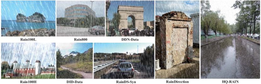
Figure 2: Example images from previous representative datasets [8, 35, 36, 5, 29, 74] and our proposed HQ-RAIN.

Full-Reference Metrics

. The commonly used full-reference IQA metrics include Peak Signal-to-Noise Ratio (PSNR) [21], Structure Similarity Index (SSIM) [117], Feature Similarity (FSIM) [118], and Learned Perceptual Image Patch Similarity (LPIPS) [119]. The PSNR assesses the pixel-level similarity between two images, whereas the SSIM measures similarity according to structure information. The FSIM and LPIPS measure similarity at the feature level between image pairs for quality evaluation. Note that, higher PSNR, SSIM, FSIM, and lower LPIPS indicate better image visual quality.

Non-Reference Metrics

. In terms of the rainy images without ground truth images, the non-reference IQA indicators are used for quantitatively evaluate the restoration performance, including Natural Image Quality Evaluator (NIQE) [120], Blind/Referenceless Image Spatial Quality Evaluator (BRISQUE) [121], and Spatial-Spectral Entropy-based Quality (SSEQ) [122]. The smaller scores of NIQE, BRISQUE and SSEQ indicate clearer contents and better perceptual quality.

User Study

. User study is a representative subjective evaluation method. Users can choose the image with the best deraining performance from a group of images. The premise is to anonymize the method and randomly sort the images in each group to ensure fairness. In general, the user study score is the mean opinion score (MOS) from a group of participants. A high MOS indicates superior perceptual quality from human perspectives.

Model Efficiency

. Model efficiency is critical driver for the practical application of deep image deraining algorithms. The evaluation metrics for model efficiency typically include the numbers of parameters (#Params), inference running time, and Floating Point Operations (FLOPs). It is widely known that a shorter running time and a smaller #Params and FLOPs means better model efficiency.

Application-based Evaluations

. One of the goals of image deraining, in addition to enhancing the visual quality, is to serve high-level vision tasks, such as object recognition [123] and segmentation [124]. Thus, to verify the performance of different methods, the effects of image deraining on outdoor vision based applications are further investigated.

Robust Analyses on Adversarial Attacks

. Rain highly degrades in a variety of ways, and the deraining model may suffer from a performance loss due to scene inconsistencies. Adversarial attacks try to degrade the deraining algorithms’ output by adding a small quantity of visually undetectable disturbances to the input rainy images. Recent studies [125, 126] have investigated various types of adversarial attacks focusing on rain degradation problems and their impact on both human and machine vision tasks.

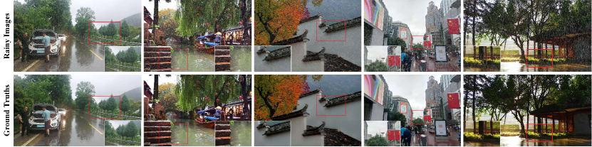
Figure 3: More example image pairs sampled from the proposed HQ-RAIN. Best viewed by zooming in the figures.

4 HQ-RAIN: A New Benchmark

Although lots of single image deraining datasets have been proposed, the quality of most synthetic rain dataset is sub-optimal in terms of realism and harmony. As a result, a large domain gap exists between synthetic and real data, thereby limiting the capacity to train better deep deraining models. In the following, we first describe the construction of the new benchmark and then compare it with other commonly used image deraining datasets.

4.1 Dataset Construction

Existing approaches usually add rain streaks into the clear images to obtain rainy images. However, this will leads to unnatural results as shown in Figure 2, especially in the sky region. Instead of simply adding rain streaks into the clear images, we develop an effective image synthesization approach to obtain more realistic datasets. Our method include the background collection, rain streaks synthesis, and image blending, which will be presented in the follows.

Background Collection

. The quality of clear backgrounds (i.e., ground-truth images) is equally significant for constructing paired datasets, which was not taken into account in previous studies. In other words, the existing synthetic datasets [8, 36, 5, 18, 74] only focus on the synthesized rain while ignoring the high-quality backgrounds that we also need. On the one hand, the ground-truths of these datasets have some unexpected problems about the images: low resolution, watermark, compression artifact, which may interfere with the quality of model learning and high-quality image reconstruction. On the other hand, they often overlook the basic fact that rainy weather mostly occurs under cloudy or low background brightness imaging conditions. When revisiting the rainy images in the existing datasets, we find that there are very obvious rain streaks in the clear blue sky region, which makes them look incompatible.

To ensure more realistic and harmonious synthetic rainy images for the next step, our selection of ground-truths is based on a strict set of collection criteria. Specifically, we first collect clear and rain-free scenes using a Python program based on Scrapy to download images from Google search. In addition, we also elaborately select several backgrounds covering abundant scenes from the DPED [127] and RainDS [29] datasets. Low quality images that contain poor resolution, website watermark, compression artifact and blur are filtered out. All clear blue sky regions are filtered out as well to ensure appropriate background composition. Here, we tend to choose suitable rain-free backgrounds based on human visual perception of real rainy days by considering sky, illumination, and ground conditions. Overall, our ground-truths covers a large variety of typical daylight and night scenes from urban locations (e.g., streets, buildings, cityscapes) to natural scenery (e.g., hills, lakes, vegetations). Similar to [16], despite the fact that our collection of ground-truths is reliant on streamers, Google Image’s fair use clause permits for its distribution to the academic community.

Rain Streaks Synthesis

. The fidelity and diversity of rain are two key factors in the rain streaks synthesis step. For convenience, most synthesis methods [5] adopt Photoshop software to render the streaks. However, this manual synthesis based method is time-consuming and labor-intensive. Inspired by [128, 129], we model the generation of rain streak layers as the motion blur process, which naturally takes advantage of two crucial aspects of rain streaks: repeatability and directionality. Mathematically, it can be expressed as:

$$\mathbf{S}=\mathbf{K}(l,\theta,w)*\mathbf{N}(n),$$ (19)

where $\mathbf{N}$ denotes the rain mask generated by random noise $n$. Here, we use uniform random numbers and thresholds to control the level of noise. $l$ and $\theta$ are the length and angle of the motion blur kernel $\mathbf{K}\in\mathbbm{R}^{p\times p}$. We further add the rotated diagonal kernel using Gaussian blur to make the rain thickness $w$. The noise quantity $n$, rain length $l$, rain angle $\theta$, and rain thickness $w$ are obtained by sampling from $[100,300]$, $[20,40]$, $[40^{\circ},120^{\circ}]$, and $[3,7]$, respectively. $*$ represents the spatial convolution operator.

Although in different synthesis methods the rain streaks are simulated and visually similar to humans, our method exhibits more flexible and higher rain diversity, which have great effect on the coverage of real-world rain.

Image Blending

. Most existing synthetic rainy images add rain streaks linearly to the rain-free backgrounds, which can easily make the composite image look unnatural, especially in the sky area. Our goal is to ensure the visual realism and harmony of synthesized rainy images, thereby reducing the domain gap between the synthetic and real images, which is never explored before. Thus, instead of directly copy-and-pasting, we adopt image blending [130] technique to yield a synthesized image. Compared to image harmonization task [22], due to the similarity of rain streaks, we do not need to accurately depict objects for the blending mask [131]. To this end, alpha blending is utilized to process the rain layer and background layer, where the alpha value of a pixel in a given layer indicates how much of the colors from lower levels may be visible through the color at that level. Formally, it can be defined as follows:

$$\mathbf{R}_{r,g,b}=\alpha\odot\mathbf{S}+(1-\alpha)\odot\mathbf{B},$$ (20)

where $\alpha$ is the blending ratio. Here, we set $\alpha$ to $[0.8,0.9]$. $\odot$ denotes the element-wise multiplication operator. Noted that $R$, $G$, and $B$ channels are processed separately.

Benchmark Statistics

. As a result, we propose a new single image deraining benchmark with high-quality backgrounds, diverse rain streaks, and harmonious layer blending, called HQ-RAIN. In total, the training and testing set of the HQ-RAIN contains 4,500 and 500 synthetic images, respectively. The average resolution of all images is $1367\times 931$. See Figure 3 for several image pairs in HQ-RAIN.

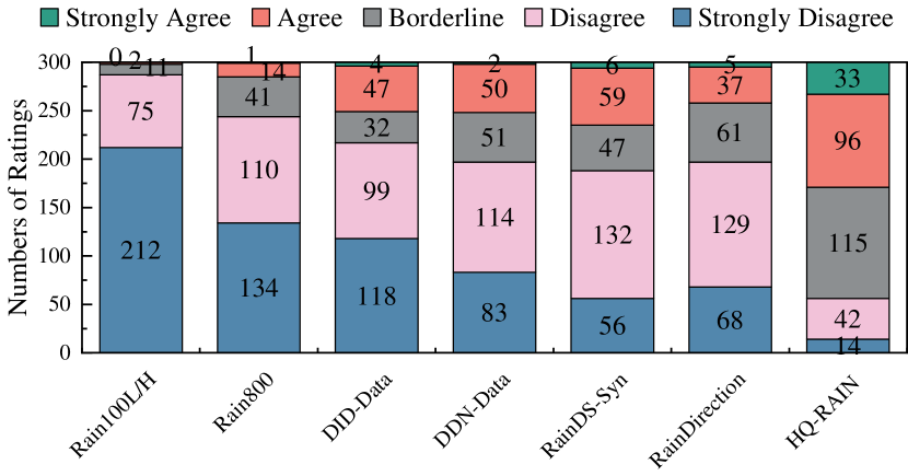
Figure 4: User study results. The ratings given by all participants on different synthesis datasets.

We also propose another new realistic dataset named RE-RAIN, to uniformly evaluate generalization performance of deraining models. Although several unlabeled real datasets have been collected [45, 132], there are some drawbacks that have the negative effects on the evaluation of generalization performance. For one thing, these real datasets contain some low-resolution images with watermarks, as well as unusual images from other bad weather conditions, which is beyond the scope of research on removing rain. For another, some rainy images have too light rain streaks, making it difficult to recognize their rain regions and thus unable to effectively evaluate deraining performance. To this end, we create a high-quality real benchmark RE-RAIN for evaluating real-world image deraining, containing 300 real rainy images without ground truths which are elaborately selected from the Internet and related works [74].

4.2 Comparisons with Previous Datasets

Subjective Assessment

. We conduct an online user study to evaluate the quality (i.e., how realistic) of the synthesis rainy images. Following the [70], we prepare for 70 rainy images, randomly chosen from 7 datasets (i.e., Rain100L/H [8], Rain800 [5], DID-Data [36], DDN-Data [35], RainDS-Syn [29], RainDirection [74] and HQ-RAIN) with 10 samples from each dataset. We recruit 30 participants with 15 males and 15 females. For each participant, we randomly show them 70 rainy images. Then, using a 5-point Likert scale (i.e., strongly agree, agree, borderline, disagree, and strongly disagree), all participants are asked to judge how realistic each image looks. Finally, 300 ratings are received for each category. Figure 4 shows the user study results. Our HQ-RAIN consistently outperforms other benchmarks, which also reveals that our synthetic rain is evaluated to be substantially more realistic than previous datasets.

TABLE III: Dataset descriptions of mixed training track and independent training track.

Tracks	Mixed Training Track							Independent Training Track
Source Datasets	Rain800 [5]	Rain100H [8]	Rain100L [8]	Rain14000 [35]	Rain1200 [35]	Rain12 [31]	Total	Rain200L [8]	Rain200H [8]	DID-Data [35]	DDN-Data [35]	SPA-Data [15]
Train Samples	700	1800	0	11,200	0	12	13712	1800	1800	12,000	12,600	638,492
Test Samples	100	100	100	2800	1200	0	4300	200	200	1,200	1,400	1,000
Name	Test100	Rain100H	Rain100L	Test2800	Test1200	-	-	Rain200L	Rain200H	DID-Data	DDN-Data	SPA-Data

Objective Assessment

. In addition to subjective assessment, we also conduct objective comparisons to verify the high quality of our proposed dataset. Here, we adopt the Kullback-Leibler Divergence (KLD) [133], also known as relative entropy, to measure the difference between two probability distributions (i.e., the synthetic image and real-world image). Figure 5 presents the comparison results of the representative synthetic benchmarks [8, 5, 36, 35] and our benchmark, showing that our HQ-RAIN are close to the distribution of real-world rainy images. The reason behind this is that HQ-RAIN fully considers the harmony of the synthesized rainy images, thereby narrowing the domain gap between synthetic and real images. We hope our benchmark can provide new impetus for future research.

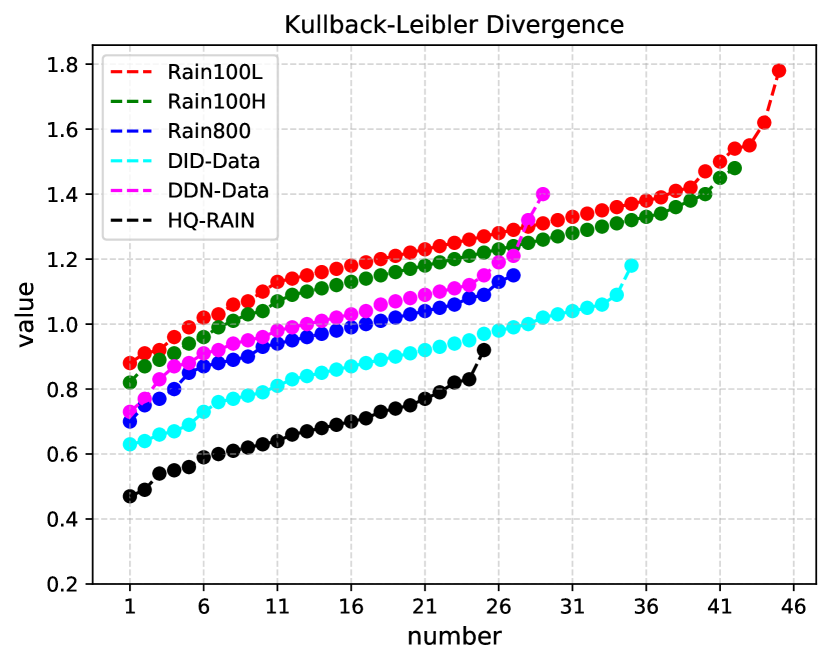
Figure 5: Comparison of Kullback CLeibler divergence (KLD) between different synthetic datasets and one real dataset. The vertical axis represents the value of KLD, and the horizontal axis represents the number of samples. Obviously, our proposed HQ-RAIN obtains a lowest KLD score, indicating that our dataset has a smaller domain gap between the synthetic and real-world images compared to others.

5 Comprehensive Evaluations and Analysis

In this section, we provide empirical analysis and conduct extensive evaluations of representative methods on several datasets and our proposed benchmark. In addition, we develop an online platform to provide the off-the-shelf toolkit, involving the large-scale performance evaluation.

5.1 Track Establishment and Evaluated Methods

For a comprehensive performance evaluation, we first select previously representative benchmarks to participate in our survey. Faced with dozens of existing benchmarks, it is not rare that we feel confused about which dataset to choose for the experiment at hand. In fact, our goal is to enable models to learn better generalization from representative datasets. To this end, we perform cross-domain generalizability validation on the commonly used datasets using same deep model Restormer [20]. Table IV shows that methods trained on the Rain13K [18] generalizes to an unseen samples well, due to the data diversity. In addition, a single dataset can also achieve the best results in certain specific scenarios, such as DDN-Data $\rightarrow$ RainDS-Real-RS. In other words, mixed datasets have advantages in comprehensive deraining performance, while single dataset has advantages in image-specific (e.g., heavy rain) deraining performance.

TABLE IV: Cross-domain generalizability analysis. Training Set $\rightarrow$ Testing Set means training on the dataset X and testing on the dataset Y.

Training Set $\rightarrow$ Testing Set	PSNR	SSIM	Avg.PSNR	Avg.SSIM
- $\rightarrow$ RainDS-Syn-RS	22.47	0.6765	23.02	0.6640
- $\rightarrow$ RainDS-Real-RS	23.58	0.6515
Rain100L $\rightarrow$ RainDS-Syn-RS	23.41	0.7026	23.33	0.6754
Rain100L $\rightarrow$ RainDS-Real-RS	23.25	0.6483
Rain100H $\rightarrow$ RainDS-Syn-RS	26.19	0.8502	24.90	0.7544
Rain100H $\rightarrow$ RainDS-Real-RS	23.62	0.6587
Rain200L $\rightarrow$ RainDS-Syn-RS	23.48	0.7085	23.40	0.6796
Rain200L $\rightarrow$ RainDS-Real-RS	23.32	0.6507
Rain200H $\rightarrow$ RainDS-Syn-RS	26.33	0.8599	25.00	0.7600
Rain200H $\rightarrow$ RainDS-Real-RS	23.68	0.6601
DID-Data $\rightarrow$ RainDS-Syn-RS	26.93	0.7699	25.56	0.7175
DID-Data $\rightarrow$ RainDS-Real-RS	24.19	0.6652
DDN-Data $\rightarrow$ RainDS-Syn-RS	29.02	0.8193	26.88	0.7543
DDN-Data $\rightarrow$ RainDS-Real-RS	24.74	0.6893
SPA-Data $\rightarrow$ RainDS-Syn-RS	22.65	0.7226	23.29	0.6924
SPA-Data $\rightarrow$ RainDS-Real-RS	23.93	0.6623
GT-RAIN $\rightarrow$ RainDS-Syn-RS	22.33	0.7088	22.80	0.6919
GT-RAIN $\rightarrow$ RainDS-Real-RS	23.28	0.6750
Rain13K $\rightarrow$ RainDS-Syn-RS	30.83	0.8890	27.78	0.7889
Rain13K $\rightarrow$ RainDS-Real-RS	24.73	0.6889

To intuitively compare the deraining results under these two different training modes, we create two main tracks, i.e., mixed training track and independent training track. For mixed training track, we adopt Rain13K benchmark [18] as the track participant. For independent training track, we find that Rain200L/H can help method generalize well than Rain100L/H, because Rain200L/H avoids the problem of duplicate image backgrounds in the training and testing sets in the old version. According to the generalization gain in Table IV, we finally adopt Rain200L/H [8], DID-Data [35], DDN-Data [35] and SPA-Data [15] as this track participants. Note that currently these two tracks only consider general rain removal, and do not include the datasets created for new tasks, such as RainKITTI2012/2015 [63] in stereo image deraining. In each track, the usage setting of training and testing datasets, as well as the measurement criteria, are the same. The detailed usage descriptions are tabulated in Table III. In what follows, we will report the benchmarking results of representative methods on these two tracks.

TABLE V: Quantitative comparisons on the Rain13K mixed benchmark dataset. Top $1_{st}$ and $2_{nd}$ results are marked in red and blue respectively.

Methods	Test100 [5]		Rain100H [8]		Rain100L [8]		Test2800 [35]		Test1200 [35]		Average
	PSNR $\uparrow$	SSIM $\uparrow$	PSNR $\uparrow$	SSIM $\uparrow$	PSNR $\uparrow$	SSIM $\uparrow$	PSNR $\uparrow$	SSIM $\uparrow$	PSNR $\uparrow$	SSIM $\uparrow$	PSNR $\uparrow$	SSIM $\uparrow$
Inputs	22.54	0.686	13.55	0.378	26.90	0.838	24.35	0.782	23.63	0.732	22.19	0.683
DerainNet [34]	22.77	0.810	14.92	0.592	27.03	0.884	24.31	0.861	23.38	0.835	22.48	0.796
SIRR [45]	22.35	0.788	16.56	0.486	25.03	0.842	24.43	0.782	26.05	0.822	22.88	0.744
DIDMDN [36]	22.56	0.818	17.35	0.524	25.23	0.741	28.13	0.867	29.95	0.901	24.58	0.770
UMRL [44]	24.41	0.829	26.01	0.832	29.18	0.923	29.97	0.905	30.55	0.910	28.02	0.880
RESCAN [38]	25.00	0.835	26.36	0.786	29.80	0.881	31.29	0.904	30.51	0.882	28.59	0.857
PReNet [42]	24.81	0.851	26.77	0.858	32.44	0.950	31.75	0.916	31.36	0.911	29.42	0.897
MSPFN [18]	27.50	0.876	28.66	0.860	32.40	0.933	32.82	0.930	32.39	0.916	30.75	0.903
MPRNet [19]	30.27	0.897	30.41	0.890	36.40	0.965	33.64	0.938	32.91	0.916	32.73	0.921
HINet [134]	30.26	0.905	30.63	0.893	37.20	0.969	33.87	0.940	33.01	0.918	33.00	0.925
SPAIR [75]	30.35	0.909	30.95	0.892	36.93	0.969	33.34	0.936	33.04	0.922	32.91	0.926
KiT [135]	30.26	0.904	30.47	0.897	36.65	0.969	33.85	0.941	32.81	0.918	32.81	0.929
DGUNet [82]	30.32	0.899	30.66	0.891	37.42	0.969	33.68	0.938	33.23	0.920	33.06	0.923
DGUNet+ [82]	30.86	0.907	31.06	0.897	38.25	0.974	34.01	0.942	33.08	0.916	33.46	0.927
MAXIM-2S [83]	31.17	0.922	30.81	0.903	38.06	0.977	33.80	0.943	32.37	0.922	33.24	0.933
Restormer [20]	32.00	0.923	31.46	0.904	38.99	0.978	34.18	0.944	33.19	0.926	33.96	0.935

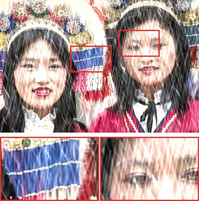
(a) Rainy Input

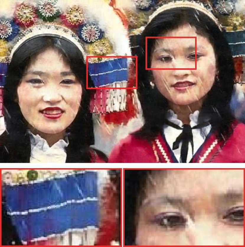
(b) RESCAN

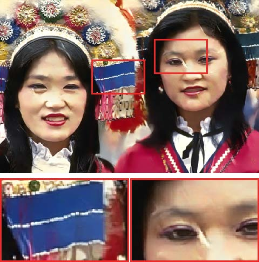
(c) PReNet

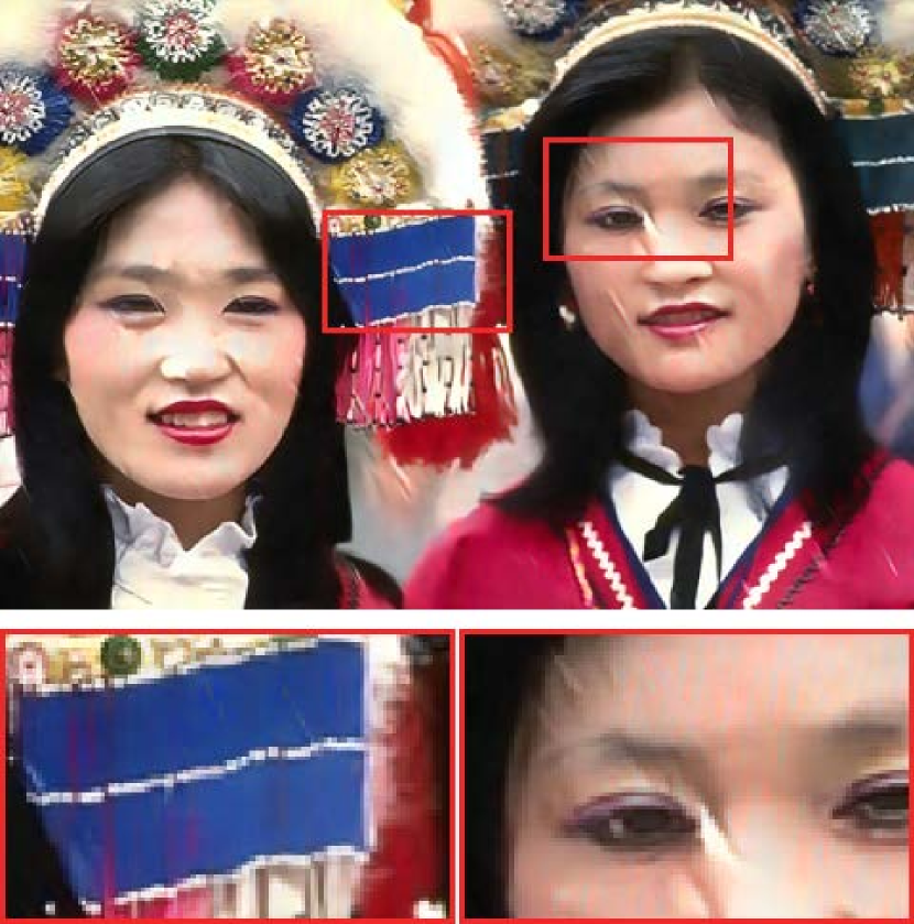
(d) MSPFN

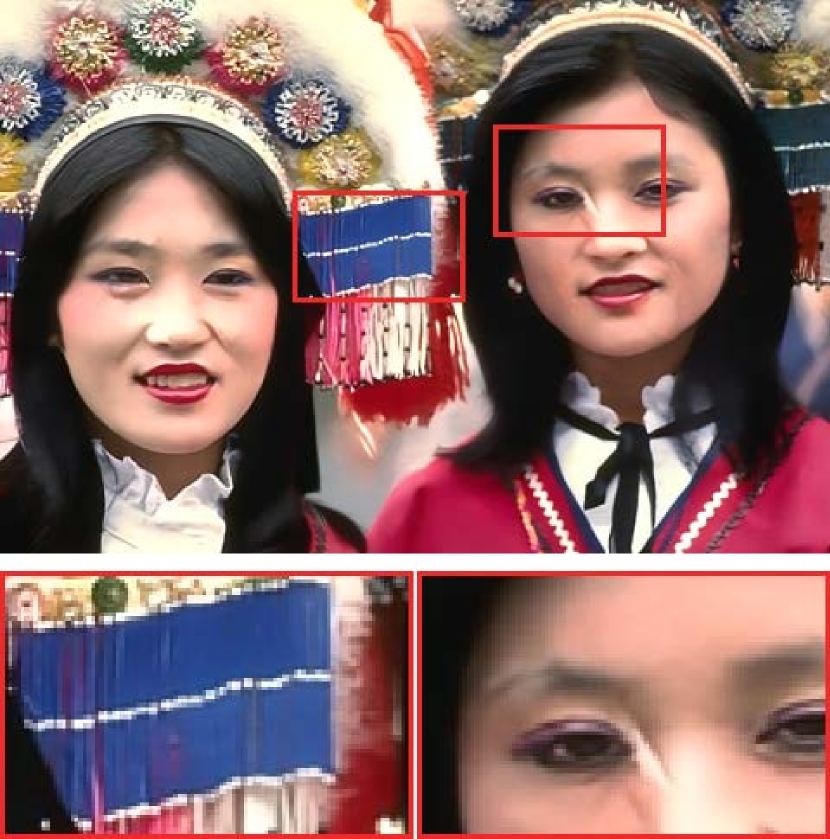
(e) MPRNet

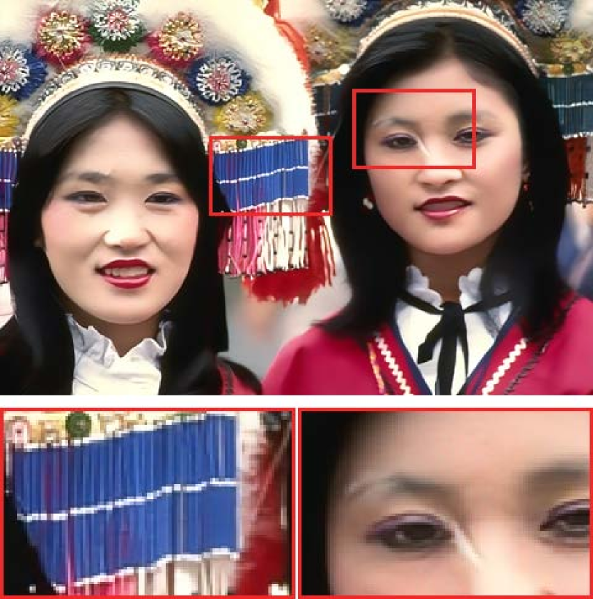
(f) DGUNet

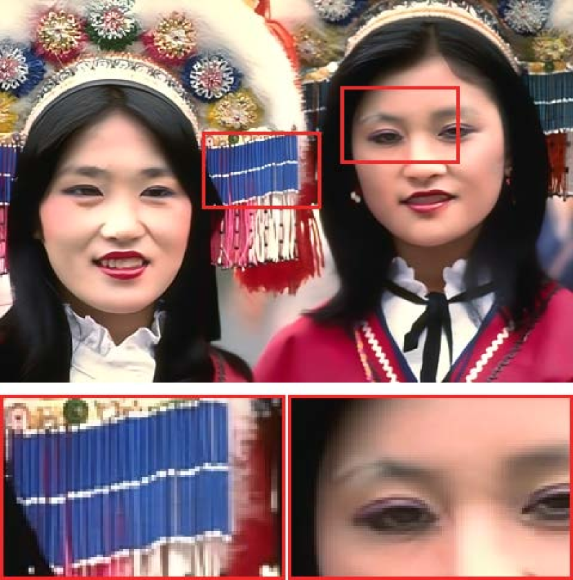
(g) DGUNet+

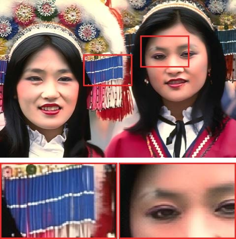
(h) MAXIM-2S

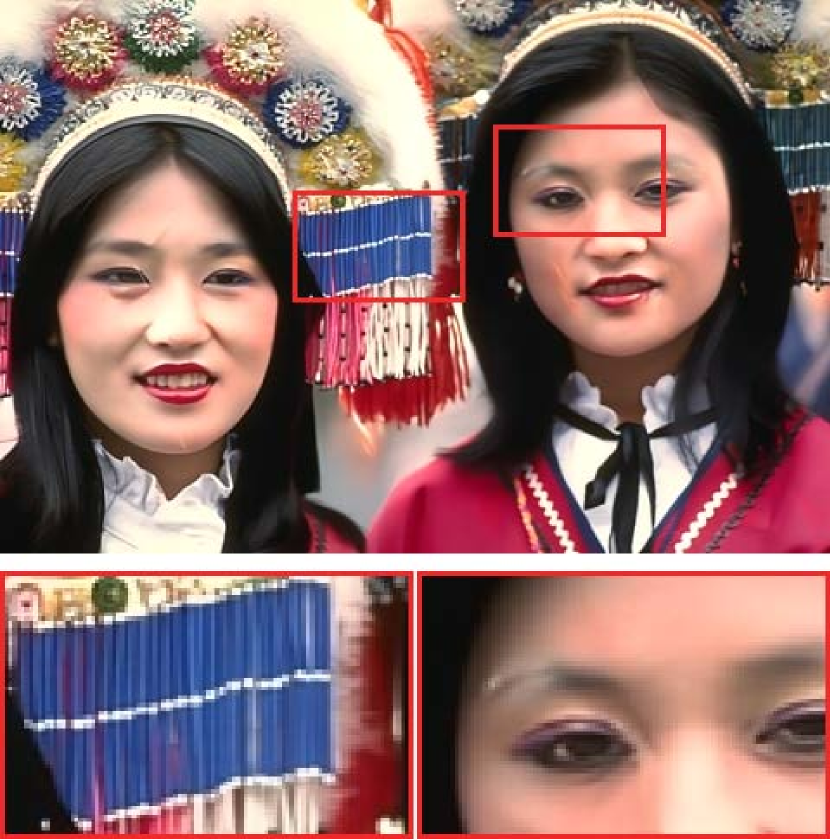
(i) Restormer

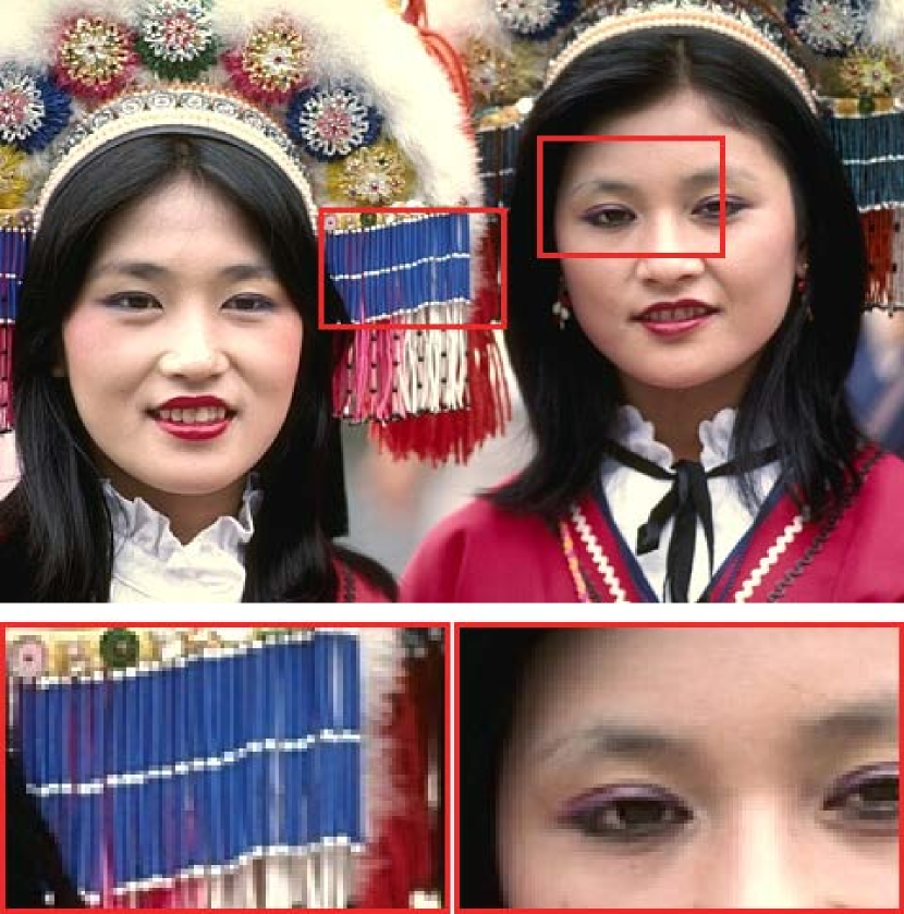
(j) Ground Truth

Figure 6: Visual quality comparison of mixed training track on the Rain100H dataset. Please zoom in the figures for better view of the rain removal and detail recovery.

5.2 Evaluation on Mixed Training Track

In this track, a pretrained model is obtained to evaluate multiple testing sets, including Test100 [5], Rain100H [8], Rain100L [8], Test2800 [35], and Test1200 [35]. From statistics in Table I, we find that this track is highly favored by image restoration task, thanks to the convenience of training on this track, which facilitates rapid evaluation of deraining performance. Here, we report 15 representative methods in Table V, i.e., DerainNet [34], SIRR [45], DIDMDN [36], UMRL [44], RESCAN [38], PReNet [42], MSPFN [18], MPRNet [19], HINet [134], SPAIR [75], KiT [135], DGUNet [82], DGUNet+ [82], MAXIM-2S [83], and Restormer [20]. Each method is evaluated under the same implementation using two well-known used indicators: PSNR [21] and SSIM [117].

So far, Restormer [20] has achieved the state-of-the-art quantitative average results in the mixed training track. In addition, DGUNet+ [82] obtained the second best average PSNR value, while MAXIM-2S [83] achieved the second best average SSIM score. Furthermore, we also present the visual comparison and the examples are shown in Figure 6. It can be seen that Transformers-based methods (e.g., MAXIM-2S [83] and Restormer [20]) can achieve significant improvement compared to the previous CNN models, as they can model the non-local information which is vital for high-quality image reconstruction. However, all approaches still need to break through in terms of image detail recovery.

TABLE VI: Results of independent training track. Quantitative comparisons on five previous commonly used benchmark datasets. Top $1_{st}$ and $2_{nd}$ results are marked in red and blue respectively.

Methods	Rain200L [8]		Rain200H [8]		DID-Data [36]		DDN-Data [35]		SPA-Data [15]		Average
	PSNR $\uparrow$	SSIM $\uparrow$	PSNR $\uparrow$	SSIM $\uparrow$	PSNR $\uparrow$	SSIM $\uparrow$	PSNR $\uparrow$	SSIM $\uparrow$	PSNR $\uparrow$	SSIM $\uparrow$	PSNR $\uparrow$	SSIM $\uparrow$
Inputs	26.71	0.8438	13.08	0.3734	23.64	0.7794	25.24	0.8098	34.14	0.9415	24.56	0.7496
DDN [35]	34.68	0.9671	26.05	0.8056	30.97	0.9116	30.00	0.9041	36.16	0.9457	31.57	0.9068
DID-MDN [36]	35.40	0.9618	26.61	0.8242	31.30	0.9207	31.49	0.9146	38.16	0.9763	32.59	0.9195
RESCAN [38]	36.09	0.9697	26.75	0.8353	33.38	0.9417	31.94	0.9345	38.11	0.9707	33.25	0.9304
NLEDN [39]	39.13	0.9821	29.79	0.9005	34.68	0.9583	32.15	0.9398	42.97	0.9835	35.74	0.9528
JORDER-E [53]	37.25	0.9752	29.35	0.8905	33.98	0.9502	32.01	0.9321	40.78	0.9801	34.67	0.9456
ID-CGAN [48]	35.19	0.9694	25.02	0.8430	30.25	0.9217	29.06	0.9162	38.47	0.9624	31.59	0.9225
SIRR [45]	34.75	0.9690	26.55	0.8190	30.57	0.9104	30.01	0.9078	35.31	0.9411	31.43	0.9095
PReNet [42]	37.80	0.9814	29.04	0.8991	33.17	0.9481	32.60	0.9459	40.16	0.9816	34.55	0.9512
SPANet [15]	35.79	0.9653	26.27	0.8666	33.04	0.9489	29.85	0.9117	40.24	0.9811	33.03	0.9347
FBL [62]	39.02	0.9827	30.07	0.9021	34.26	0.9320	33.05	0.9334	42.80	0.9824	35.84	0.9465
MSPFN [18]	38.58	0.9827	29.36	0.9034	33.72	0.9550	32.99	0.9333	43.43	0.9843	35.61	0.9517
RCDNet [57]	39.17	0.9885	30.24	0.9048	34.08	0.9532	33.04	0.9472	43.36	0.9831	35.97	0.9554
Syn2Real [58]	35.92	0.9709	27.90	0.8605	32.39	0.9390	29.29	0.9057	35.28	0.9745	32.15	0.9301
SGCN [104]	37.95	0.9822	29.35	0.9055	33.58	0.9477	32.14	0.9364	43.84	0.9862	35.37	0.9516
MPRNet [19]	39.47	0.9825	30.67	0.9110	33.99	0.9590	33.10	0.9347	43.64	0.9844	36.17	0.9543
DualGCN [13]	40.73	0.9886	31.15	0.9125	34.37	0.9620	33.01	0.9489	44.18	0.9902	36.68	0.9604
SPDNet [12]	40.50	0.9875	31.28	0.9207	34.57	0.9560	33.15	0.9457	43.20	0.9871	36.54	0.9594
Uformer [81]	40.20	0.9860	30.80	0.9105	35.02	0.9621	33.95	0.9545	46.13	0.9913	37.22	0.9609
Restormer [20]	40.99	0.9890	32.00	0.9329	35.29	0.9641	34.20	0.9571	47.98	0.9921	38.09	0.9670
IDT [11]	40.74	0.9884	32.10	0.9344	34.89	0.9623	33.84	0.9549	47.35	0.9930	37.78	0.9666
HCN [10]	41.31	0.9892	31.34	0.9248	34.70	0.9613	33.42	0.9512	45.03	0.9907	37.16	0.9634
DRSformer [9]	41.23	0.9894	32.17	0.9326	35.35	0.9646	34.35	0.9588	48.54	0.9924	38.32	0.9676

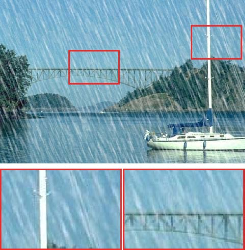
(a) Rainy Input

(b) PReNet

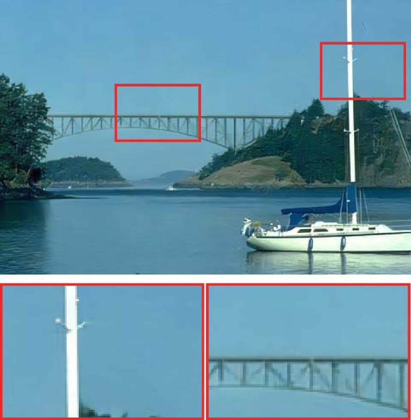
(c) RCDNet

(d) DualGCN

(e) SPDNet

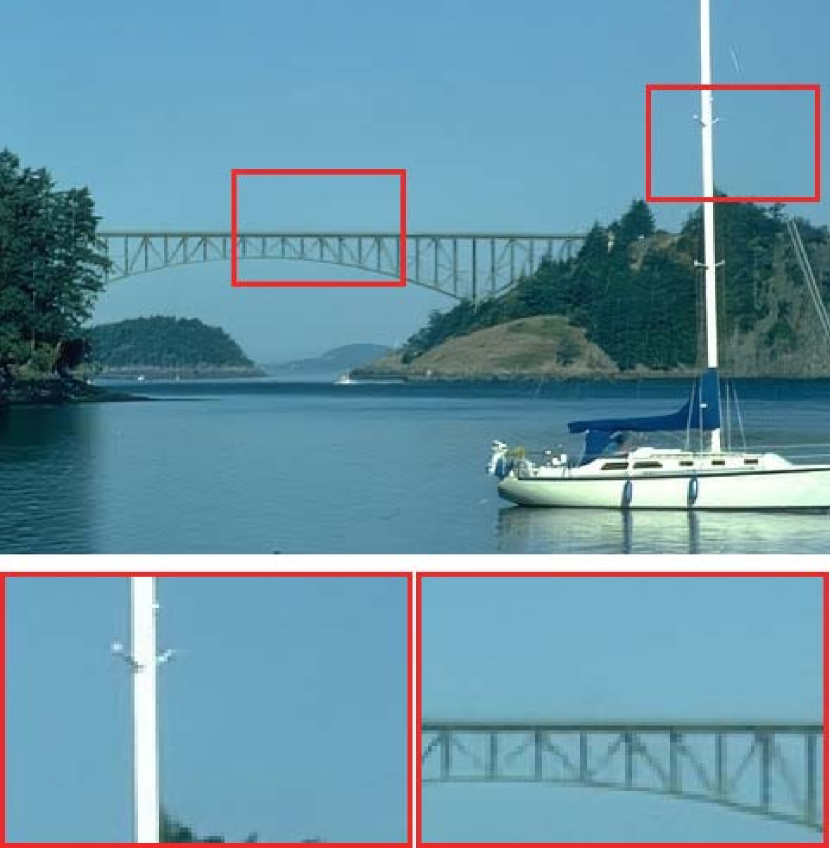
(f) Uformer

(g) Restormer

(h) IDT

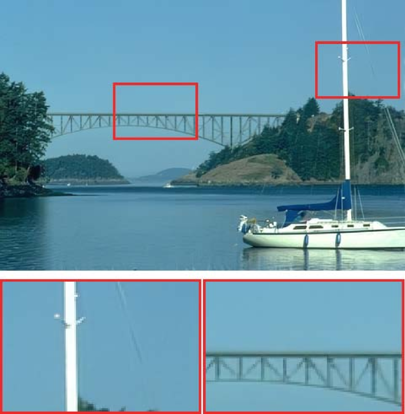
(i) DRSformer

(j) Ground Truth

Figure 7: Visual quality comparison of independent training track on the DDN-Data dataset. Please zoom in the figures for better view of the rain removal and detail recovery.

5.3 Evaluation on Independent Training Track

In this track, multiple pretrained models are obtained to evaluate the corresponding testing sets, including Rain200L [8], Rain200H [8], DID-Data [36], DDN-Data [35], and SPA-Data [15]. Here, we provide 22 representative methods in Table VI, i.e., DDN [35], DID-MDN [36], RESCAN [38], NLEDN [39], JORDER-E [53], ID-CGAN [48], SIRR [45], PReNet [42], SPANet [15], FBL [62], MSPFN [18], RCDNet [57], Syn2Real [58], SGCN [104], MPRNet [19], DualGCN [13], SPDNet [12], Uformer [81], Restormer [20], IDT [11], HCN [10], and DRSformer [9]. The quantitative results are quoted from previous works [10, 9]. Each method is evaluated under the same implementation using PSNR [21] and SSIM [117].

So far, DRSformer [9] achieves the state-of-the-art quantitative average results in the independent training track. We can note that the best performance of different methods gradually converges. The performance gaps between DRSformer [9], Restormer [20] and IDT [11] are considerably close. We further present qualitative comparisons of deraining results in Figure 7, where the “spar” shares similar directions and distributions to rain streaks. Notably, none of the methods can preserve the original details of the image content area while removing the rain streaks. Overall, there is still a certain gap between these results and ground truths.

TABLE VII: Quantitative comparisons on the HQ-RAIN and RE-RAIN benchmark datasets. Top $1_{st}$ and $2_{nd}$ results are marked in red and blue respectively. “#FLOPs”, “#Params” and “#Runtime” represent FLOPs (in G), the number of trainable parameters (in M) and inference time (in second), respectively.

Methods	LPNet [52]	PReNet [42]	JORDER-E [53]	RCDNet [57]	HINet [134]	SPDNet [12]	Uformer [81]	Restormer [20]	IDT [11]	DRSformer [9]
Benchmark	HQ-RAIN
PSNR $\uparrow$	31.39	36.73	36.46	39.53	42.30	34.02	37.57	44.59	38.38	44.67
SSIM $\uparrow$	0.9203	0.9657	0.9599	0.9771	0.9841	0.9359	0.9673	0.9905	0.9737	0.9898
LPIPS $\downarrow$	0.1024	0.0350	0.0435	0.0242	0.0147	0.0813	0.0314	0.0076	0.0261	0.0081
Benchmark	RE-RAIN
NIQE $\downarrow$	5.550	5.619	5.401	5.658	5.784	5.405	5.370	5.864	5.683	5.857
PIQE $\downarrow$	13.787	13.324	13.716	13.813	13.418	14.249	13.473	13.623	13.746	13.678
BRISQUE $\downarrow$	24.863	28.180	25.436	28.006	29.003	26.134	26.491	29.725	28.330	29.747
#FLOPs (G) $\downarrow$	3.5	66.4	27.2	21.2	170.7	89.3	45.9	174.7	61.9	242.9
#Params (M) $\downarrow$	0.03	0.17	4.21	3.17	88.67	3.04	50.88	26.12	16.41	33.65
#Runtime (s) $\downarrow$	0.07	0.09	0.25	0.26	0.38	0.24	0.21	0.28	0.28	0.30

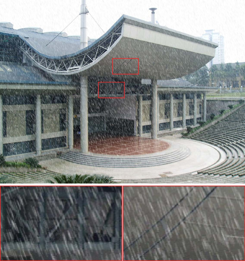
(a) Rainy Input

(b) LPNet

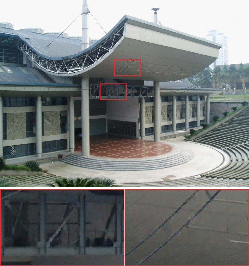
(c) PReNet

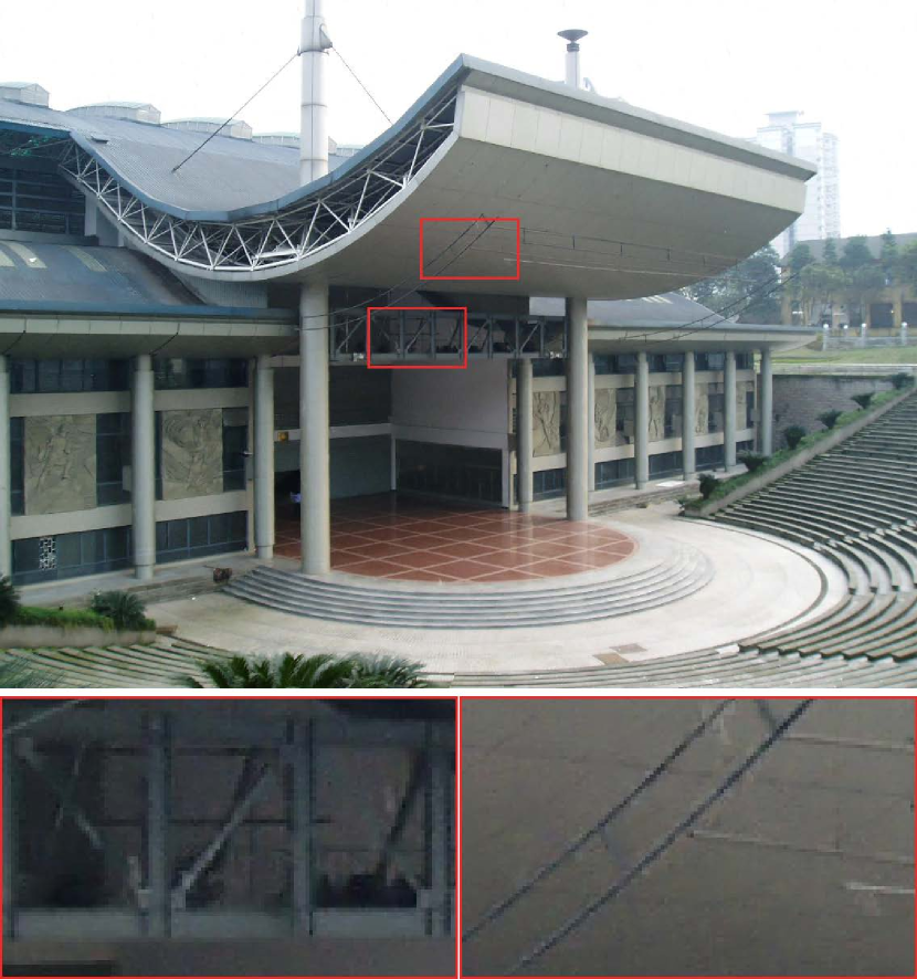
(d) JORDER-E

(e) RCDNet

(f) HINet

(g) SPDNet

(h) Uformer

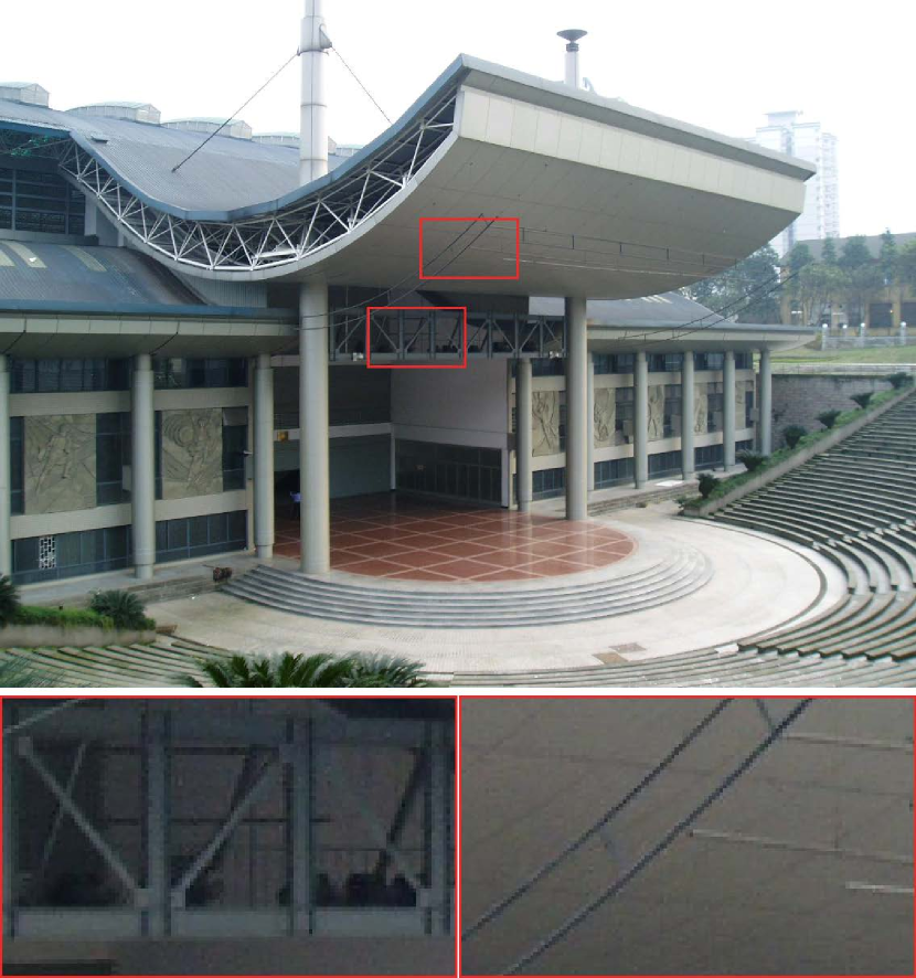
(i) Restormer

(j) IDT

(k) DRSformer

(l) Ground Truth

Figure 8: Visual quality comparison of new benchmark track on the HQ-RAIN dataset. Please zoom in the figures for better view of the rain removal and detail recovery.

5.4 Evaluation on the HQ-RAIN Dataset

We further conduct experiments on the proposed new benchmark to evaluate the performance of existing methods. Specifically, we select 10 representative methods including 6 CNN-based approaches (i.e., LPNet [52], PReNet [42], JORDER-E [53], RCDNet [57], HINet [134] and SPDNet [12]) and 4 Transformer-based methods (i.e., Uformer [81], Restormer [20], IDT [11] and DRSformer [9]) for evaluation. For fair comparisons, we use the official released codes of these approaches. All methods are retrained on the HQ-RAIN benchmark. We choose their best pre-trained models, which achieve the highest PSNR value on the HQ-RAIN testing set. Meanwhile, these pre-trained models also are used to validate the RE-RAIN benchmark. All experiments are implemented on the servers equipped with NVIDIA GeForce RTX 3090 GPUs. For the HQ-RAIN benchmark with ground truth images, we use PSNR [21], SSIM [117], and LPIPS [119] to evaluate the quality of each restored images. For the RE-RAIN benchmark without ground truth images, we use the non-reference metrics including NIQE [120], PIQE [136], and BRISQUE [121]. Higher PSNR and SSIM scores indicate higher restoration quality, while lower LPIPS, NIQE, PIQE and BRISQUE values indicate better perceptual quality. The above-mentioned metrics are calculated based on the Y channel in YCbCr space of derained images for fair comparisons.

Table VII demonstrates quantitative results of all methods on the HQ-RAIN and RE-RAIN benchmarks. We note that DRSformer [9] and Restormer [20] obtain the top two performance on the synthetic HQ-RAIN benchmark. However, they do not perform well on the real-world RE-RAIN benchmark, which means that these two methods do generalize well on real-world applications. In addition, among the CNN-based methods, HINet [134] achieves the competitive results on the HQ-RAIN. As some specific domain knowledge is beneficial for real-world rain removal [57], intergrading some specific domain knowledge into the model designs improves the generalization ability of deep learning. The results on the RE-RAIN demonstrate that most CNN-based methods have better generalization performance than Transformer-based methods as most CNN-based approaches integrate domain knowledge (e.g., rain structure and kernel) to better guide the model designs. Figures 8 and 9 show several visual comparisons. The DRSformer [9] performs better than the evaluated methods, which keeps consistent with the above quantitative results. Figure 9 show that LPNet [52] generates better derained images. Based on above evaluations, deraining real-world images is challenging and worthy further studied.

TABLE VIII: Quantitative comparisons of mAP and mAR under different IoU thresholds of downstream object detection task. Top $1_{st}$ and $2_{nd}$ results are marked in red and blue respectively.

Methods	LPNet [52]	PReNet [42]	JORDER-E [53]	RCDNet [57]	HINet [134]	SPDNet [12]	Uformer [81]	Restormer [20]	IDT [11]	DRSformer [9]
	IoU threshold=0.5
mAP $\uparrow$	0.480	0.507	0.542	0.556	0.566	0.469	0.573	0.499	0.541	0.556
mAR $\uparrow$	0.704	0.699	0.698	0.739	0.732	0.657	0.736	0.687	0.736	0.735
	IoU threshold=0.6
mAP $\uparrow$	0.333	0.375	0.429	0.430	0.379	0.381	0.425	0.426	0.388	0.397
mAR $\uparrow$	0.560	0.469	0.575	0.617	0.507	0.471	0.606	0.641	0.474	0.482
	IoU threshold=0.7
mAP $\uparrow$	0.249	0.291	0.285	0.306	0.299	0.291	0.300	0.305	0.301	0.301
mAR $\uparrow$	0.363	0.364	0.357	0.374	0.368	0.359	0.362	0.375	0.367	0.372

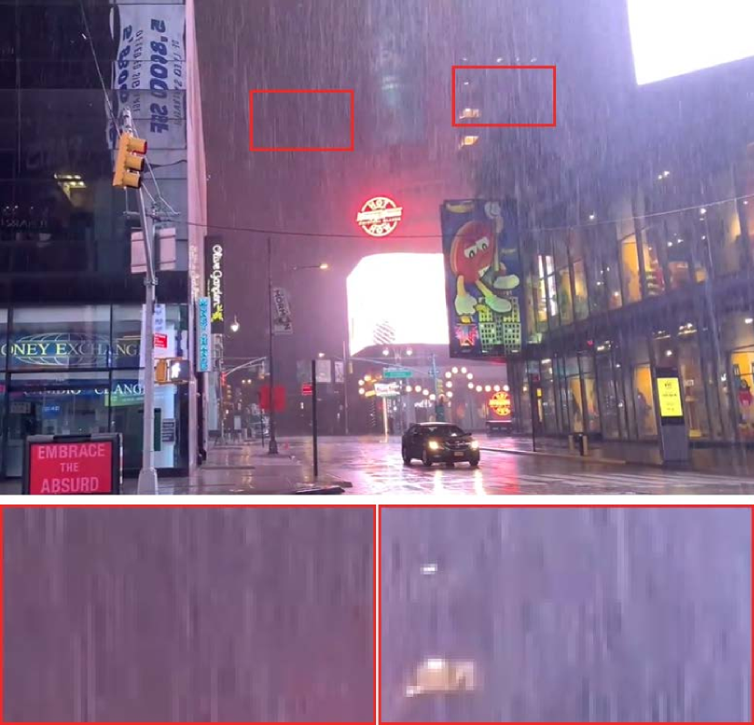
(a) Rainy Input

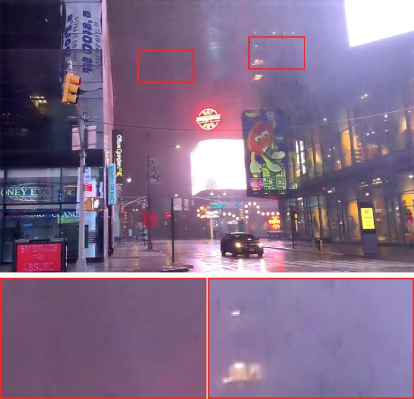
(b) LPNet

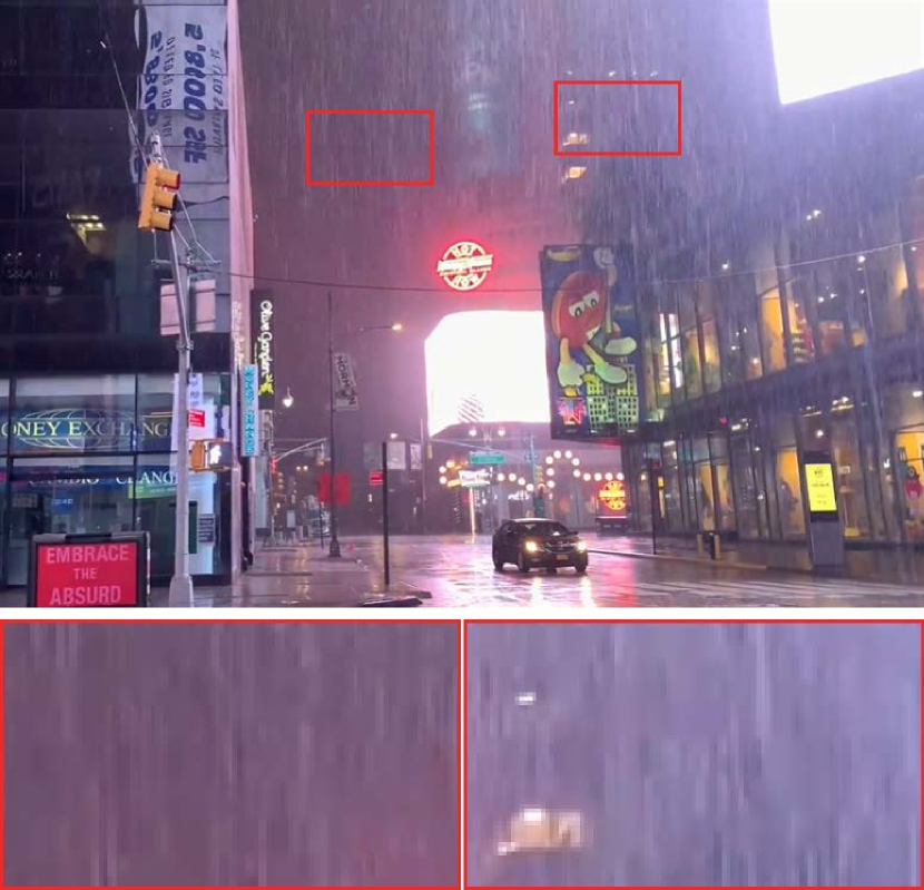
(c) PReNet

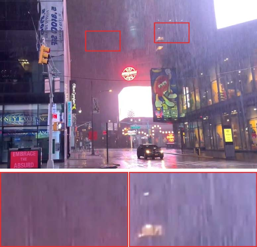
(d) JORDER-E

(e) RCDNet

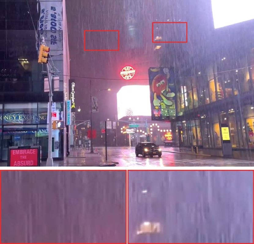
(f) HINet

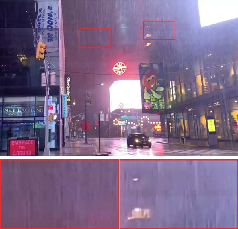
(g) SPDNet

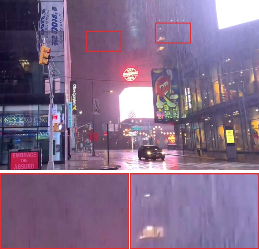
(h) Uformer

(i) IDT

(j) DRSformer

Figure 9: Visual quality comparison of new benchmark track on the RE-RAIN dataset. Please zoom in the figures for better view of the rain removal and detail recovery.

5.5 Computational Complexity

The computational complexity is also one of the important factor for image deaining methods. Table VII shows the computational complexity of different methods, including trainable model parameters, FLOPs and running time on a $256\times 256$ image. LPNet [52] requires lower computational complexity as it develops a lightweight pyramid network using domain-specific knowledge to simplify the learning process. In contrast, the model size of HINet [134] is extremely large, reaching 88.67M, which limits its usage in practical applications. The FLOPs of DRSformer [9] is relatively higher as it involves the computation of the top-k self-attention. For inference time, most existing methods, especially Transformer-based approaches, are not efficient. Thus, how to develop efficient yet effective method is still worthy investigation.

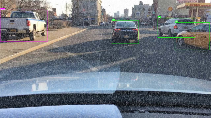
(a) Rainy Input

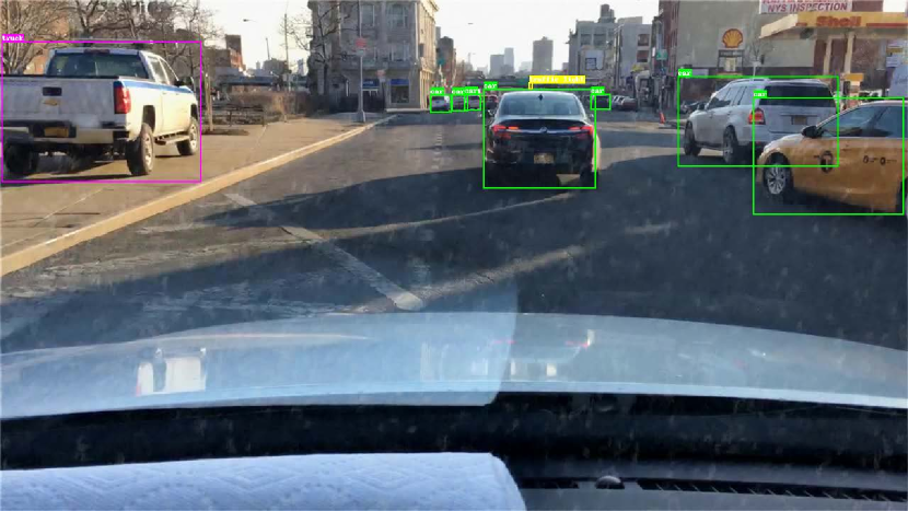
(b) PReNet

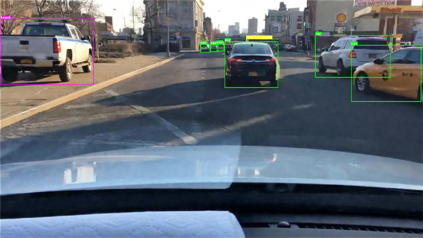
(c) JORDER-E

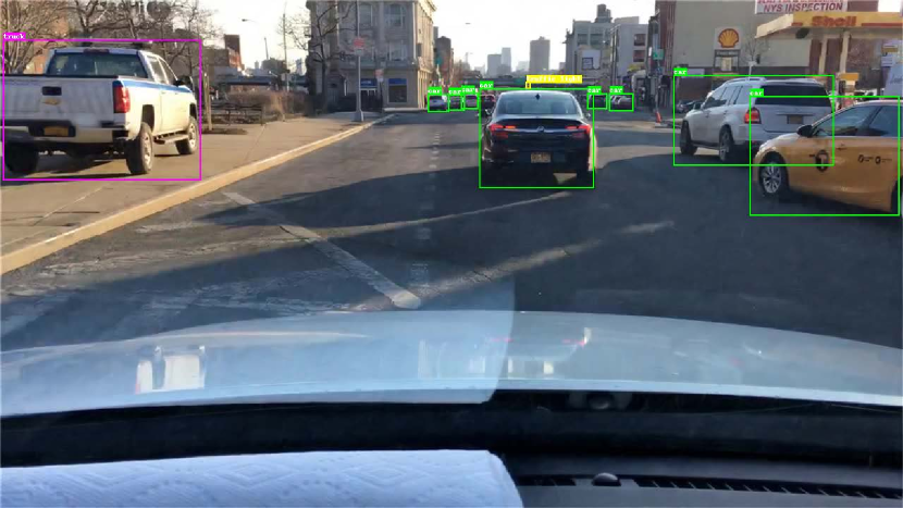
(d) RCDNet

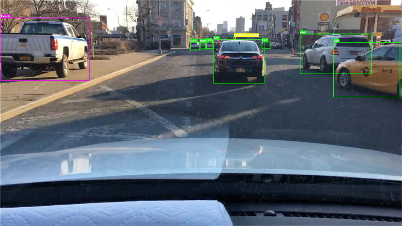
(e) HINet

(f) SPDNet

(g) Uformer

(h) Restormer

(i) IDT

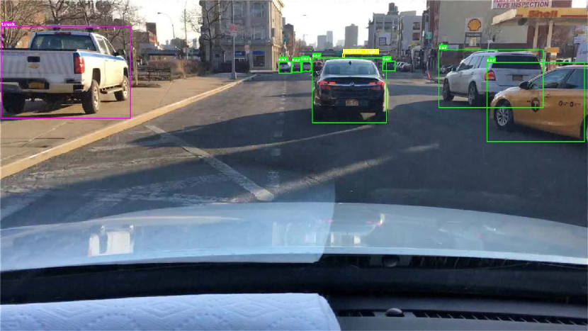
(j) DRSformer

Figure 10: Visual comparison of joint image deraining and object detection. Please zoom in the figures for better view of the rain removal and object detection.

(a) Survey Page

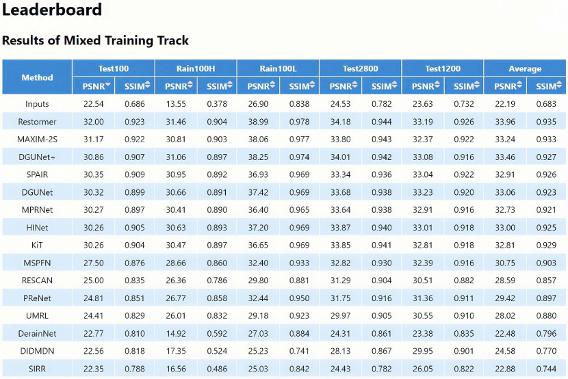
(b) Leaderboard Page

(c) Submit Page

Figure 11: Screenshots of the developed online evaluation platform. Some design styles refer to the SIDD website [137].

5.6 Application-Based Evaluation

To investigate whether the image deraining process benefits downstream vision-based applications, e.g., object detection, we apply the popular object detection pre-trained model (YOLOv3 [138]) to evaluate the deraining results. Here, we create a high-quality version of BDD350 (joint image deraining and object detection) [87]. Following [139], we calculate the mean Average Precision (mAP) and mean Average Recall (mAR) under different Intersection of Union (IoU) thresholds using the available evaluation tool. In addition, visual comparisons are presented in Figure 10. As one can see, the detection precision of the deraining results by all algorithms shows different degrees of improvement over that of original rainy inputs. From Table VIII, RCDNet [57] surprisingly achieves relatively robust performance on the object detection. This may be because this method can better protect the image semantic information by using an interpretable rain dictionary model. However, some recent methods (e.g., IDT [11] and DRSformer [9]) exhibit rapid performance degradation under higher threshold setting, suggesting that there are still rooms for improvement.

5.7 Online Evaluation Platform

To facilitate the large-scale evaluation and tracking of the latest deraining technologies for general users, we develop an online platform for current research development of image deraining. Figure 11 shows some screenshots of the proposed online evaluation platform. The proposed evaluation platform provides a comprehensive repository, including direct links and source codes for 100 representative methods, to continuously track recent developments in this fast-advancing field. It also provides evaluations of several popular and representative image deraining methods to better facilitate the following researches. In addition, the evaluation platform allows users submit the derained results and can provide direct comparisons with existing methods online. More visual results on the mixed training track, independent training track and new benchmark can also be downloaded on our platform. The proposed online evaluation platform is updated regularly to report new technology trends and benchmark results.

6 Future Research Prospects

Single image deraining has undergone rapid development in recent years, thanks to the incorporation of deep learning techniques. Researchers have made significant contributions by proposing effective models, promoting the optimization process, and establishing abundant datasets to advance the field. Despite achieving promising results, there are still several opportunities to explore in this field including how to model the degradation process, effective deraining models, and its potential applications for the following image analysis tasks.

6.1 Degradation Progress

The degradation progress models the generation of the rainy images. Thus, how to better model the degradation progress is critical for image deraining in the deep learning era. As the real degradation is complex, the image synthesization based on the linear composition model, e.g., (1), may not be able to model the real degradation. The methods trained on the datasets based on the linear composition model may not generalize well on real-world applications due to the domain gap of the data distributions.

Although several approaches design kinds of hardwares to capture real-world rainy images, the diversity of images and complexity of rainy environments (e.g., low-light environment, hazy environment, and so on) are not sufficient to cover the realistic scenarios. Therefore, how to describe the degradation of clear image in rainy settings including the rainy streak distributions, rainy image properties, the laws of physics of rain and so on is a great of need but still challenging.

6.2 Model Development

High-quality Image Deraining Models.

As image deraining aims to recover realistic clear images, how to develop an effective model that describes the properties of clear image is important. Below we will present some promising directions for network improvements. (1) Integrating domain knowledge into model development. For instance, by leveraging semantic segmentation, we can identify specific regions of interest in the image such as sky or roads [140]. This may allow us to use unequal information from different regions to guide the model in removing rain and avoiding unnecessary information loss. (2) Modeling the distributions of clear images. We can use image generation approaches (e.g., VQGAN [141] or diffusion models [100]) to facilitate the high-quality image restoration. (3) Exploring external information of clear images or distilling the knowledge from large pre-trained models to facilitate the rain removal. By prompt learning or knowledge distillation, the model can benefit from the learned representations and generalization capabilities. This allows the model to effectively utilize the specific prompts or knowledge to better understand and remove rain from images.

Efficient Image Deraining Models.

Developing efficient image deraining models is important due to resource-limited devices in most real-world applications. Facing this challenge, we can adopt pruning [142], dimension reduction and feature reuse [143] to remove unnecessary connections or parameters from the network. In addition, knowledge distillation [144] can also be used to facilitate the transfer of knowledge from a complex model to a compact one, effectively compressing the model while maintaining performance. We can also explore neural architecture search [145] to learn compact models by introducing various search strategies to sample architectures from the defined search space.

6.3 Potential Applications

Relations of Image Deraining and Other Tasks.

Most existing methods mainly focuses on the individual image deraining task and usually use the image deraining task as a pre- or post-processing step for other tasks. Although the development of these fields are independent, different tasks can have a constructive influence in promoting each other, such as Deblur-YOLO [146] and YOLO-in-the-Dark [147]. We call for closer collaboration across low-level and high-level communities.

7 Concluding Remarks

We have provided comprehensive overview of the existing image deraining methods. We first analyze the research progress, discuss the limitations, and provide empirical evaluations of image deraining methods. To better evaluate existing methods, we propose develop a rainy image generation approach based on an image harmonization approach and develop a realistic image deraining dataset. We have established two parallel tracks (i.e., mixed training track and independent training track) to facilitate effective and fair performance comparison among different methods. We carry out qualitative and quantitative analyses to investigate the open challenges and provide the future prospects. To provide fair evaluation protocols, we build an online platform to better evaluate the deraining methods and facilitate the following researches. The online evaluation platform is publicly available and will be regularly updated.

References

- [1] W. Sultani, C. Chen, and M. Shah, “Real-world anomaly detection in surveillance videos,” in Proceedings of the IEEE Conference on Computer Vision and Pattern Recognition, 2018, pp. 6479–6488.
- [2] B. R. Kiran, I. Sobh, V. Talpaert, P. Mannion, A. A. Al Sallab, S. Yogamani, and P. Pérez, “Deep reinforcement learning for autonomous driving: A survey,” IEEE Transactions on Intelligent Transportation Systems, 2021.
- [3] M. Ye, J. Shen, G. Lin, T. Xiang, L. Shao, and S. C. Hoi, “Deep learning for person re-identification: A survey and outlook,” IEEE Transactions on Pattern Analysis and Machine Intelligence, vol. 44, no. 6, pp. 2872–2893, 2021.
- [4] H. Wang, Y. Wu, M. Li, Q. Zhao, and D. Meng, “A survey on rain removal from video and single image,” arXiv preprint arXiv:1909.08326, 2019.
- [5] S. Li, I. B. Araujo, W. Ren, Z. Wang, E. K. Tokuda, R. H. Junior, R. Cesar-Junior, J. Zhang, X. Guo, and X. Cao, “Single image deraining: A comprehensive benchmark analysis,” in Proceedings of the IEEE Conference on Computer Vision and Pattern Recognition, 2019, pp. 3838–3847.
- [6] W. Yang, R. T. Tan, S. Wang, Y. Fang, and J. Liu, “Single image deraining: From model-based to data-driven and beyond,” IEEE Transactions on Pattern Analysis and Machine Intelligence, vol. 43, no. 11, pp. 4059–4077, 2020.
- [7] Z. Zhang, Y. Wei, H. Zhang, Y. Yang, S. Yan, and M. Wang, “Data-driven single image deraining: a comprehensive review and new perspectives,” Pattern Recognition, p. 109740, 2023.
- [8] W. Yang, R. T. Tan, J. Feng, J. Liu, Z. Guo, and S. Yan, “Deep joint rain detection and removal from a single image,” in Proceedings of the IEEE Conference on Computer Vision and Pattern Recognition, 2017, pp. 1357–1366.
- [9] X. Chen, H. Li, M. Li, and J. Pan, “Learning a sparse transformer network for effective image deraining,” in Proceedings of the IEEE Conference on Computer Vision and Pattern Recognition, 2023, pp. 5896–5905.
- [10] X. Fu, J. Xiao, Y. Zhu, A. Liu, F. Wu, and Z.-J. Zha, “Continual image deraining with hypergraph convolutional networks,” IEEE Transactions on Pattern Analysis and Machine Intelligence, 2023.
- [11] J. Xiao, X. Fu, A. Liu, F. Wu, and Z.-J. Zha, “Image de-raining transformer,” IEEE Transactions on Pattern Analysis and Machine Intelligence, 2022.
- [12] Q. Yi, J. Li, Q. Dai, F. Fang, G. Zhang, and T. Zeng, “Structure-preserving deraining with residue channel prior guidance,” in Proceedings of the IEEE International Conference on Computer Vision, 2021, pp. 4238–4247.
- [13] X. Fu, Q. Qi, Z.-J. Zha, Y. Zhu, and X. Ding, “Rain streak removal via dual graph convolutional network,” in Proceedings of the AAAI Conference on Artificial Intelligence, 2021, pp. 1352–1360.
- [14] S. Deng, M. Wei, J. Wang, Y. Feng, L. Liang, H. Xie, F. L. Wang, and M. Wang, “Detail-recovery image deraining via context aggregation networks,” in Proceedings of the IEEE Conference on Computer Vision and Pattern Recognition, 2020, pp. 14 560–14 569.
- [15] T. Wang, X. Yang, K. Xu, S. Chen, Q. Zhang, and R. W. Lau, “Spatial attentive single-image deraining with a high quality real rain dataset,” in Proceedings of the IEEE Conference on Computer Vision and Pattern Recognition, 2019, pp. 12 270–12 279.
- [16] Y. Ba, H. Zhang, E. Yang, A. Suzuki, A. Pfahnl, C. C. Chandrappa, C. M. de Melo, S. You, S. Soatto, A. Wong et al., “Not just streaks: Towards ground truth for single image deraining,” in Proceedings of the European Conference on Computer Vision, 2022, pp. 723–740.
- [17] W. Li, Q. Zhang, J. Zhang, Z. Huang, X. Tian, and D. Tao, “Toward real-world single image deraining: A new benchmark and beyond,” arXiv preprint arXiv:2206.05514, 2022.
- [18] K. Jiang, Z. Wang, P. Yi, C. Chen, B. Huang, Y. Luo, J. Ma, and J. Jiang, “Multi-scale progressive fusion network for single image deraining,” in Proceedings of the IEEE Conference on Computer Vision and Pattern Recognition, 2020, pp. 8346–8355.
- [19] S. W. Zamir, A. Arora, S. Khan, M. Hayat, F. S. Khan, M.-H. Yang, and L. Shao, “Multi-stage progressive image restoration,” in Proceedings of the IEEE Conference on Computer Vision and Pattern Recognition, 2021, pp. 14 821–14 831.
- [20] S. W. Zamir, A. Arora, S. Khan, M. Hayat, F. S. Khan, and M.-H. Yang, “Restormer: Efficient transformer for high-resolution image restoration,” in Proceedings of the IEEE Conference on Computer Vision and Pattern Recognition, 2022, pp. 5728–5739.
- [21] Q. Huynh-Thu and M. Ghanbari, “Scope of validity of psnr in image/video quality assessment,” Electronics Letters, vol. 44, no. 13, pp. 800–801, 2008.
- [22] W. Cong, J. Zhang, L. Niu, L. Liu, Z. Ling, W. Li, and L. Zhang, “Dovenet: Deep image harmonization via domain verification,” in Proceedings of the IEEE Conference on Computer Vision and Pattern Recognition, 2020, pp. 8394–8403.
- [23] Y. Luo, Y. Xu, and H. Ji, “Removing rain from a single image via discriminative sparse coding,” in Proceedings of the IEEE International Conference on Computer Vision, 2015, pp. 3397–3405.
- [24] E. J. McCartney, “Optics of the atmosphere: scattering by molecules and particles,” New York, 1976.
- [25] X. Hu, C.-W. Fu, L. Zhu, and P.-A. Heng, “Depth-attentional features for single-image rain removal,” in Proceedings of the IEEE Conference on Computer Vision and Pattern Recognition, 2019, pp. 8022–8031.
- [26] Y. Wang, Y. Song, C. Ma, and B. Zeng, “Rethinking image deraining via rain streaks and vapors,” in Proceedings of the European Conference on Computer Vision, 2020, pp. 367–382.
- [27] S. You, R. T. Tan, R. Kawakami, Y. Mukaigawa, and K. Ikeuchi, “Adherent raindrop modeling, detection and removal in video,” IEEE Transactions on Pattern Analysis and Machine Intelligence, vol. 38, no. 9, pp. 1721–1733, 2015.
- [28] R. Qian, R. T. Tan, W. Yang, J. Su, and J. Liu, “Attentive generative adversarial network for raindrop removal from a single image,” in Proceedings of the IEEE Conference on Computer Vision and Pattern Recognition, 2018, pp. 2482–2491.
- [29] R. Quan, X. Yu, Y. Liang, and Y. Yang, “Removing raindrops and rain streaks in one go,” in Proceedings of the IEEE Conference on Computer Vision and Pattern Recognition, 2021, pp. 9147–9156.
- [30] L.-W. Kang, C.-W. Lin, and Y.-H. Fu, “Automatic single-image-based rain streaks removal via image decomposition,” IEEE Transactions on Image Processing, vol. 21, no. 4, pp. 1742–1755, 2011.
- [31] Y. Li, R. T. Tan, X. Guo, J. Lu, and M. S. Brown, “Rain streak removal using layer priors,” in Proceedings of the IEEE Conference on Computer Vision and Pattern Recognition, 2016, pp. 2736–2744.
- [32] L. Zhu, C.-W. Fu, D. Lischinski, and P.-A. Heng, “Joint bi-layer optimization for single-image rain streak removal,” in Proceedings of the IEEE International Conference on Computer Vision, 2017, pp. 2526–2534.
- [33] S. Gu, D. Meng, W. Zuo, and L. Zhang, “Joint convolutional analysis and synthesis sparse representation for single image layer separation,” in Proceedings of the IEEE International Conference on Computer Vision, 2017, pp. 1708–1716.
- [34] X. Fu, J. Huang, X. Ding, Y. Liao, and J. Paisley, “Clearing the skies: A deep network architecture for single-image rain removal,” IEEE Transactions on Image Processing, vol. 26, no. 6, pp. 2944–2956, 2017.
- [35] X. Fu, J. Huang, D. Zeng, Y. Huang, X. Ding, and J. Paisley, “Removing rain from single images via a deep detail network,” in Proceedings of the IEEE Conference on Computer Vision and Pattern Recognition, 2017, pp. 3855–3863.
- [36] H. Zhang and V. M. Patel, “Density-aware single image de-raining using a multi-stream dense network,” in Proceedings of the IEEE Conference on Computer Vision and Pattern Recognition, 2018, pp. 695–704.
- [37] J. Pan, S. Liu, D. Sun, J. Zhang, Y. Liu, J. Ren, Z. Li, J. Tang, H. Lu, Y.-W. Tai et al., “Learning dual convolutional neural networks for low-level vision,” in Proceedings of the IEEE Conference on Computer Vision and Pattern Recognition, 2018, pp. 3070–3079.
- [38] X. Li, J. Wu, Z. Lin, H. Liu, and H. Zha, “Recurrent squeeze-and-excitation context aggregation net for single image deraining,” in Proceedings of the European Conference on Computer Vision, 2018, pp. 254–269.
- [39] G. Li, X. He, W. Zhang, H. Chang, L. Dong, and L. Lin, “Non-locally enhanced encoder-decoder network for single image de-raining,” in Proceedings of the 26th ACM International Conference on Multimedia, 2018, pp. 1056–1064.
- [40] Z. Fan, H. Wu, X. Fu, Y. Huang, and X. Ding, “Residual-guide network for single image deraining,” in Proceedings of the 26th ACM International Conference on Multimedia, 2018, pp. 1751–1759.
- [41] D. Chen, M. He, Q. Fan, J. Liao, L. Zhang, D. Hou, L. Yuan, and G. Hua, “Gated context aggregation network for image dehazing and deraining,” in Proceedings of the IEEE Winter Conference on Applications of Computer Vision, 2019, pp. 1375–1383.
- [42] D. Ren, W. Zuo, Q. Hu, P. Zhu, and D. Meng, “Progressive image deraining networks: A better and simpler baseline,” in Proceedings of the IEEE Conference on Computer Vision and Pattern Recognition, 2019, pp. 3937–3946.
- [43] R. Li, L.-F. Cheong, and R. T. Tan, “Heavy rain image restoration: Integrating physics model and conditional adversarial learning,” in Proceedings of the IEEE Conference on Computer Vision and Pattern Recognition, 2019, pp. 1633–1642.
- [44] R. Yasarla and V. M. Patel, “Uncertainty guided multi-scale residual learning-using a cycle spinning cnn for single image de-raining,” in Proceedings of the IEEE Conference on Computer Vision and Pattern Recognition, 2019, pp. 8405–8414.
- [45] W. Wei, D. Meng, Q. Zhao, Z. Xu, and Y. Wu, “Semi-supervised transfer learning for image rain removal,” in Proceedings of the IEEE Conference on Computer Vision and Pattern Recognition, 2019, pp. 3877–3886.
- [46] Y. Quan, S. Deng, Y. Chen, and H. Ji, “Deep learning for seeing through window with raindrops,” in Proceedings of the IEEE Conference on Computer Vision and Pattern Recognition, 2019, pp. 2463–2471.
- [47] G. Wang, C. Sun, and A. Sowmya, “Erl-net: Entangled representation learning for single image de-raining,” in Proceedings of the IEEE International Conference on Computer Vision, 2019, pp. 5644–5652.
- [48] H. Zhang, V. Sindagi, and V. M. Patel, “Image de-raining using a conditional generative adversarial network,” IEEE Transactions on Circuits and Systems for Video Technology, vol. 30, no. 11, pp. 3943–3956, 2019.
- [49] Z. Wang, J. Li, and G. Song, “Dtdn: Dual-task de-raining network,” in Proceedings of the 27th ACM International Conference on Multimedia, 2019, pp. 1833–1841.
- [50] W. Yu, Z. Huang, W. Zhang, L. Feng, and N. Xiao, “Gradual network for single image de-raining,” in Proceedings of the 27th ACM International Conference on Multimedia, 2019, pp. 1795–1804.
- [51] Y. Yang and H. Lu, “Single image deraining via recurrent hierarchy enhancement network,” in Proceedings of the 27th ACM International Conference on Multimedia, 2019, pp. 1814–1822.
- [52] X. Fu, B. Liang, Y. Huang, X. Ding, and J. Paisley, “Lightweight pyramid networks for image deraining,” IEEE Transactions on Neural Networks and Learning Systems, vol. 31, no. 6, pp. 1794–1807, 2019.
- [53] W. Yang, R. T. Tan, J. Feng, Z. Guo, S. Yan, and J. Liu, “Joint rain detection and removal from a single image with contextualized deep networks,” IEEE Transactions on Pattern Analysis and Machine Intelligence, vol. 42, no. 6, pp. 1377–1393, 2019.
- [54] H. Zhu, X. Peng, J. T. Zhou, S. Yang, V. Chanderasekh, L. Li, and J.-H. Lim, “Singe image rain removal with unpaired information: A differentiable programming perspective,” in Proceedings of the AAAI Conference on Artificial Intelligence, 2019, pp. 9332–9339.
- [55] X. Jin, Z. Chen, J. Lin, Z. Chen, and W. Zhou, “Unsupervised single image deraining with self-supervised constraints,” in Proceedings of the IEEE International Conference on Image Processing, 2019, pp. 2761–2765.
- [56] X. Liu, M. Suganuma, Z. Sun, and T. Okatani, “Dual residual networks leveraging the potential of paired operations for image restoration,” in Proceedings of the IEEE Conference on Computer Vision and Pattern Recognition, 2019, pp. 7007–7016.
- [57] H. Wang, Q. Xie, Q. Zhao, and D. Meng, “A model-driven deep neural network for single image rain removal,” in Proceedings of the IEEE Conference on Computer Vision and Pattern Recognition, 2020, pp. 3103–3112.
- [58] R. Yasarla, V. A. Sindagi, and V. M. Patel, “Syn2real transfer learning for image deraining using gaussian processes,” in Proceedings of the IEEE Conference on Computer Vision and Pattern Recognition, 2020, pp. 2726–2736.
- [59] R. Li, R. T. Tan, and L.-F. Cheong, “All in one bad weather removal using architectural search,” in Proceedings of the IEEE Conference on Computer Vision and Pattern Recognition, 2020, pp. 3175–3185.
- [60] Y. Du, J. Xu, X. Zhen, M.-M. Cheng, and L. Shao, “Conditional variational image deraining,” IEEE Transactions on Image Processing, vol. 29, pp. 6288–6301, 2020.
- [61] J. Pan, J. Dong, Y. Liu, J. Zhang, J. Ren, J. Tang, Y.-W. Tai, and M.-H. Yang, “Physics-based generative adversarial models for image restoration and beyond,” IEEE Transactions on Pattern Analysis and Machine Intelligence, vol. 43, no. 7, pp. 2449–2462, 2020.
- [62] W. Yang, S. Wang, D. Xu, X. Wang, and J. Liu, “Towards scale-free rain streak removal via self-supervised fractal band learning,” in Proceedings of the AAAI Conference on Artificial Intelligence, 2020, pp. 12 629–12 636.
- [63] K. Zhang, W. Luo, W. Ren, J. Wang, F. Zhao, L. Ma, and H. Li, “Beyond monocular deraining: Stereo image deraining via semantic understanding,” in Proceedings of the European Conference on Computer Vision, 2020, pp. 71–89.
- [64] C. Wang, X. Xing, Y. Wu, Z. Su, and J. Chen, “Dcsfn: Deep cross-scale fusion network for single image rain removal,” in Proceedings of the 28th ACM International Conference on Multimedia, 2020, pp. 1643–1651.
- [65] C. Wang, Y. Wu, Z. Su, and J. Chen, “Joint self-attention and scale-aggregation for self-calibrated deraining network,” in Proceedings of the 28th ACM International Conference on Multimedia, 2020, pp. 2517–2525.
- [66] Y. Wei, Z. Zhang, Y. Wang, M. Xu, Y. Yang, S. Yan, and M. Wang, “Deraincyclegan: Rain attentive cyclegan for single image deraining and rainmaking,” IEEE Transactions on Image Processing, vol. 30, pp. 4788–4801, 2021.
- [67] H. Chen, Y. Wang, T. Guo, C. Xu, Y. Deng, Z. Liu, S. Ma, C. Xu, C. Xu, and W. Gao, “Pre-trained image processing transformer,” in Proceedings of the IEEE Conference on Computer Vision and Pattern Recognition, 2021, pp. 12 299–12 310.
- [68] H. Huang, A. Yu, and R. He, “Memory oriented transfer learning for semi-supervised image deraining,” in Proceedings of the IEEE Conference on Computer Vision and Pattern Recognition, 2021, pp. 7732–7741.
- [69] C. Chen and H. Li, “Robust representation learning with feedback for single image deraining,” in Proceedings of the IEEE Conference on Computer Vision and Pattern Recognition, 2021, pp. 7742–7751.
- [70] H. Wang, Z. Yue, Q. Xie, Q. Zhao, Y. Zheng, and D. Meng, “From rain generation to rain removal,” in Proceedings of the IEEE Conference on Computer Vision and Pattern Recognition, 2021, pp. 14 791–14 801.
- [71] Y. Ye, Y. Chang, H. Zhou, and L. Yan, “Closing the loop: Joint rain generation and removal via disentangled image translation,” in Proceedings of the IEEE Conference on Computer Vision and Pattern Recognition, 2021, pp. 2053–2062.
- [72] S. Ni, X. Cao, T. Yue, and X. Hu, “Controlling the rain: From removal to rendering,” in Proceedings of the IEEE Conference on Computer Vision and Pattern Recognition, 2021, pp. 6328–6337.
- [73] Y. Wang, C. Ma, and B. Zeng, “Multi-decoding deraining network and quasi-sparsity based training,” in Proceedings of the IEEE Conference on Computer Vision and Pattern Recognition, 2021, pp. 13 375–13 384.
- [74] Y. Liu, Z. Yue, J. Pan, and Z. Su, “Unpaired learning for deep image deraining with rain direction regularizer,” in Proceedings of the IEEE International Conference on Computer Vision, 2021, pp. 4753–4761.
- [75] K. Purohit, M. Suin, A. Rajagopalan, and V. N. Boddeti, “Spatially-adaptive image restoration using distortion-guided networks,” in Proceedings of the IEEE International Conference on Computer Vision, 2021, pp. 2309–2319.
- [76] C. Yu, Y. Chang, Y. Li, X. Zhao, and L. Yan, “Unsupervised image deraining: Optimization model driven deep cnn,” in Proceedings of the 29th ACM International Conference on Multimedia, 2021, pp. 2634–2642.
- [77] Q. Guo, J. Sun, F. Juefei-Xu, L. Ma, X. Xie, W. Feng, Y. Liu, and J. Zhao, “Efficientderain: Learning pixel-wise dilation filtering for high-efficiency single-image deraining,” in Proceedings of the AAAI Conference on Artificial Intelligence, 2021, pp. 1487–1495.
- [78] H. Huang, A. Yu, Z. Chai, R. He, and T. Tan, “Selective wavelet attention learning for single image deraining,” International Journal of Computer Vision, vol. 129, pp. 1282–1300, 2021.
- [79] X. Chen, J. Pan, K. Jiang, Y. Li, Y. Huang, C. Kong, L. Dai, and Z. Fan, “Unpaired deep image deraining using dual contrastive learning,” in Proceedings of the IEEE Conference on Computer Vision and Pattern Recognition, 2022, pp. 2017–2026.
- [80] Y. Ye, C. Yu, Y. Chang, L. Zhu, X.-L. Zhao, L. Yan, and Y. Tian, “Unsupervised deraining: Where contrastive learning meets self-similarity,” in Proceedings of the IEEE Conference on Computer Vision and Pattern Recognition, 2022, pp. 5821–5830.
- [81] Z. Wang, X. Cun, J. Bao, W. Zhou, J. Liu, and H. Li, “Uformer: A general u-shaped transformer for image restoration,” in Proceedings of the IEEE Conference on Computer Vision and Pattern Recognition, 2022, pp. 17 683–17 693.
- [82] C. Mou, Q. Wang, and J. Zhang, “Deep generalized unfolding networks for image restoration,” in Proceedings of the IEEE Conference on Computer Vision and Pattern Recognition, 2022, pp. 17 399–17 410.
- [83] Z. Tu, H. Talebi, H. Zhang, F. Yang, P. Milanfar, A. Bovik, and Y. Li, “Maxim: Multi-axis mlp for image processing,” in Proceedings of the IEEE Conference on Computer Vision and Pattern Recognition, 2022, pp. 5769–5780.
- [84] B. Li, X. Liu, P. Hu, Z. Wu, J. Lv, and X. Peng, “All-in-one image restoration for unknown corruption,” in Proceedings of the IEEE Conference on Computer Vision and Pattern Recognition, 2022, pp. 17 452–17 462.
- [85] J. M. J. Valanarasu, R. Yasarla, and V. M. Patel, “Transweather: Transformer-based restoration of images degraded by adverse weather conditions,” in Proceedings of the IEEE Conference on Computer Vision and Pattern Recognition, 2022, pp. 2353–2363.
- [86] D. Lin, W. Xin, J. Shen, R. Zhang, R. Liu, M. Wang, W. Xie, Q. Guo, and P. Li, “Generative status estimation and information decoupling for image rain removal,” in Proceedings of the Advances in Neural Information Processing Systems, 2022.
- [87] K. Jiang, Z. Wang, C. Chen, Z. Wang, L. Cui, and C.-W. Lin, “Magic elf: Image deraining meets association learning and transformer,” 2022.
- [88] X. Chen, J. Pan, J. Lu, Z. Fan, and H. Li, “Hybrid cnn-transformer feature fusion for single image deraining,” in Proceedings of the AAAI Conference on Artificial Intelligence, 2023.
- [89] O. Özdenizci and R. Legenstein, “Restoring vision in adverse weather conditions with patch-based denoising diffusion models,” IEEE Transactions on Pattern Analysis and Machine Intelligence, 2023.
- [90] Y. Wang, C. Ma, and J. Liu, “Smartassign: Learning a smart knowledge assignment strategy for deraining and desnowing,” in Proceedings of the IEEE Conference on Computer Vision and Pattern Recognition, 2023, pp. 3677–3686.
- [91] K. He, J. Sun, and X. Tang, “Guided image filtering,” IEEE Transactions on Pattern Analysis and Machine Intelligence, vol. 35, no. 6, pp. 1397–1409, 2012.
- [92] J. Xu, W. Zhao, P. Liu, and X. Tang, “Removing rain and snow in a single image using guided filter,” in Proceedings of the IEEE International Conference on Computer Science and Automation Engineering, vol. 2, 2012, pp. 304–307.
- [93] ——, “An improved guidance image based method to remove rain and snow in a single image,” Computer and Information Science, vol. 5, no. 3, p. 49, 2012.
- [94] J.-H. Kim, C. Lee, J.-Y. Sim, and C.-S. Kim, “Single-image deraining using an adaptive nonlocal means filter,” in Proceedings of the IEEE International Conference on Image Processing, 2013, pp. 914–917.
- [95] X. Zheng, Y. Liao, W. Guo, X. Fu, and X. Ding, “Single-image-based rain and snow removal using multi-guided filter,” in Proceedings of the International Conference on Neural Information Processing, 2013, pp. 258–265.
- [96] X. Ding, L. Chen, X. Zheng, Y. Huang, and D. Zeng, “Single image rain and snow removal via guided l0 smoothing filter,” Multimedia Tools and Applications, vol. 75, no. 5, pp. 2697–2712, 2016.
- [97] Y.-L. Chen and C.-T. Hsu, “A generalized low-rank appearance model for spatio-temporally correlated rain streaks,” in Proceedings of the IEEE International Conference on Computer Vision, 2013, pp. 1968–1975.
- [98] I. Goodfellow, J. Pouget-Abadie, M. Mirza, B. Xu, D. Warde-Farley, S. Ozair, A. Courville, and Y. Bengio, “Generative adversarial networks,” Communications of the ACM, vol. 63, no. 11, pp. 139–144, 2020.
- [99] A. Vaswani, N. Shazeer, N. Parmar, J. Uszkoreit, L. Jones, A. N. Gomez, Ł. Kaiser, and I. Polosukhin, “Attention is all you need,” Advances in Neural Information Processing Systems, vol. 30, 2017.
- [100] J. Ho, A. Jain, and P. Abbeel, “Denoising diffusion probabilistic models,” Advances in Neural Information Processing Systems, vol. 33, pp. 6840–6851, 2020.
- [101] W. Liu, R. Jiang, C. Chen, T. Lu, and Z. Xiong, “An unsupervised attentive-adversarial learning framework for single image deraining,” arXiv preprint arXiv:2202.09635, 2022.
- [102] D. Eigen, D. Krishnan, and R. Fergus, “Restoring an image taken through a window covered with dirt or rain,” in Proceedings of the IEEE International Conference on Computer Vision, 2013, pp. 633–640.
- [103] K. He, X. Zhang, S. Ren, and J. Sun, “Deep residual learning for image recognition,” in Proceedings of the IEEE Conference on Computer Vision and Pattern Recognition, 2016, pp. 770–778.
- [104] X. Fu, Q. Qi, Z.-J. Zha, X. Ding, F. Wu, and J. Paisley, “Successive graph convolutional network for image de-raining,” International Journal of Computer Vision, vol. 129, pp. 1691–1711, 2021.
- [105] X. Chen, Z. Fan, P. Li, L. Dai, C. Kong, Z. Zheng, Y. Huang, and Y. Li, “Unpaired deep image dehazing using contrastive disentanglement learning,” in European Conference on Computer Vision, 2022, pp. 632–648.
- [106] T. R. Shaham, T. Dekel, and T. Michaeli, “Singan: Learning a generative model from a single natural image,” in Proceedings of the IEEE Conference on Computer Vision and Pattern Recognition, 2019, pp. 4570–4580.
- [107] K. Han, Y. Wang, H. Chen, X. Chen, J. Guo, Z. Liu, Y. Tang, A. Xiao, C. Xu, Y. Xu et al., “A survey on vision transformer,” IEEE Transactions on Pattern Analysis and Machine Intelligence, vol. 45, no. 1, pp. 87–110, 2022.
- [108] O. Ronneberger, P. Fischer, and T. Brox, “U-net: Convolutional networks for biomedical image segmentation,” in Proceedings of the Medical Image Computing and Computer-Assisted Intervention, 2015, pp. 234–241.
- [109] T. Chan, S. Esedoglu, F. Park, A. Yip et al., “Recent developments in total variation image restoration,” Mathematical Models of Computer Vision, vol. 17, no. 2, pp. 17–31, 2005.
- [110] P. Arbelaez, M. Maire, C. Fowlkes, and J. Malik, “Contour detection and hierarchical image segmentation,” IEEE Transactions on Pattern Analysis and Machine Intelligence, vol. 33, no. 5, pp. 898–916, 2010.
- [111] K. Garg and S. K. Nayar, “Photorealistic rendering of rain streaks,” ACM Transactions on Graphics, vol. 25, no. 3, pp. 996–1002, 2006.
- [112] G. Schaefer and M. Stich, “Ucid: An uncompressed color image database,” in Proceedings of the Storage and Retrieval Methods and Applications for Multimedia, vol. 5307, 2003, pp. 472–480.
- [113] M. Cordts, M. Omran, S. Ramos, T. Rehfeld, M. Enzweiler, R. Benenson, U. Franke, S. Roth, and B. Schiele, “The cityscapes dataset for semantic urban scene understanding,” in Proceedings of the IEEE Conference on Computer Vision and Pattern Recognition, 2016, pp. 3213–3223.
- [114] C. Godard, O. Mac Aodha, and G. J. Brostow, “Unsupervised monocular depth estimation with left-right consistency,” in Proceedings of the IEEE Conference on Computer Vision and Pattern Recognition, 2017, pp. 270–279.
- [115] A. Geiger, P. Lenz, C. Stiller, and R. Urtasun, “Vision meets robotics: The kitti dataset,” The International Journal of Robotics Research, vol. 32, no. 11, pp. 1231–1237, 2013.
- [116] R. Timofte, E. Agustsson, L. Van Gool, M.-H. Yang, and L. Zhang, “Ntire 2017 challenge on single image super-resolution: Methods and results,” in Proceedings of the IEEE Conference on Computer Vision and Pattern Recognition Workshops, 2017, pp. 114–125.
- [117] Z. Wang, A. C. Bovik, H. R. Sheikh, and E. P. Simoncelli, “Image quality assessment: from error visibility to structural similarity,” IEEE Transactions on Image Processing, vol. 13, no. 4, pp. 600–612, 2004.
- [118] L. Zhang, L. Zhang, X. Mou, and D. Zhang, “Fsim: A feature similarity index for image quality assessment,” IEEE Transactions on Image Processing, vol. 20, no. 8, pp. 2378–2386, 2011.
- [119] R. Zhang, P. Isola, A. A. Efros, E. Shechtman, and O. Wang, “The unreasonable effectiveness of deep features as a perceptual metric,” in Proceedings of the IEEE Conference on Computer Vision and Pattern Recognition, 2018, pp. 586–595.
- [120] A. Mittal, A. K. Moorthy, and A. C. Bovik, “No-reference image quality assessment in the spatial domain,” IEEE Transactions on Image Processing, vol. 21, no. 12, pp. 4695–4708, 2012.
- [121] A. Mittal, R. Soundararajan, and A. C. Bovik, “Making a “completely blind” image quality analyzer,” IEEE Signal Processing Letters, vol. 20, no. 3, pp. 209–212, 2012.
- [122] L. Liu, B. Liu, H. Huang, and A. C. Bovik, “No-reference image quality assessment based on spatial and spectral entropies,” Signal Processing: Image Communication, vol. 29, no. 8, pp. 856–863, 2014.
- [123] L. Liu, W. Ouyang, X. Wang, P. Fieguth, J. Chen, X. Liu, and M. Pietikäinen, “Deep learning for generic object detection: A survey,” International Journal of Computer Vision, vol. 128, pp. 261–318, 2020.
- [124] Z. Wojna, V. Ferrari, S. Guadarrama, N. Silberman, L.-C. Chen, A. Fathi, and J. Uijlings, “The devil is in the decoder: Classification, regression and gans,” International Journal of Computer Vision, vol. 127, pp. 1694–1706, 2019.
- [125] Y. Yu, W. Yang, Y.-P. Tan, and A. C. Kot, “Towards robust rain removal against adversarial attacks: A comprehensive benchmark analysis and beyond,” in Proceedings of the IEEE Conference on Computer Vision and Pattern Recognition, 2022, pp. 6013–6022.
- [126] J. Liu, B. Lu, M. Xiong, T. Zhang, and H. Xiong, “Adversarial attack with raindrops,” arXiv preprint arXiv:2302.14267, 2023.
- [127] A. Ignatov, N. Kobyshev, R. Timofte, K. Vanhoey, and L. Van Gool, “Dslr-quality photos on mobile devices with deep convolutional networks,” in Proceedings of the IEEE International Conference on Computer Vision, 2017, pp. 3277–3285.
- [128] K. Garg and S. K. Nayar, “Vision and rain,” International Journal of Computer Vision, vol. 75, pp. 3–27, 2007.
- [129] Y.-T. Wang, X.-L. Zhao, T.-X. Jiang, L.-J. Deng, Y. Chang, and T.-Z. Huang, “Rain streaks removal for single image via kernel-guided convolutional neural network,” IEEE Transactions on Neural Networks and Learning Systems, vol. 32, no. 8, pp. 3664–3676, 2020.
- [130] T. Porter and T. Duff, “Compositing digital images,” in Proceedings of the 11th Annual Conference on Computer Graphics and Interactive Techniques, 1984, pp. 253–259.
- [131] L. Zhang, T. Wen, and J. Shi, “Deep image blending,” in Proceedings of the IEEE Winter Conference on Applications of Computer Vision, 2020, pp. 231–240.
- [132] Y. Wei, Z. Zhang, Y. Wang, H. Zhang, M. Zhao, M. Xu, and M. Wang, “Semi-deraingan: A new semi-supervised single image deraining,” in Proceedings of the IEEE International Conference on Multimedia and Expo, 2021, pp. 1–6.
- [133] J. M. Joyce, “Kullback-leibler divergence,” in International Encyclopedia of Statistical Science, 2011, pp. 720–722.
- [134] L. Chen, X. Lu, J. Zhang, X. Chu, and C. Chen, “Hinet: Half instance normalization network for image restoration,” in Proceedings of the IEEE Conference on Computer Vision and Pattern Recognition, 2021, pp. 182–192.
- [135] H. Lee, H. Choi, K. Sohn, and D. Min, “Knn local attention for image restoration,” in Proceedings of the IEEE Conference on Computer Vision and Pattern Recognition, 2022, pp. 2139–2149.
- [136] N. Venkatanath, D. Praneeth, M. C. Bh, S. S. Channappayya, and S. S. Medasani, “Blind image quality evaluation using perception based features,” in Proceedings of the National Conference on Communications, 2015, pp. 1–6.
- [137] A. Abdelhamed, S. Lin, and M. S. Brown, “A high-quality denoising dataset for smartphone cameras,” in Proceedings of the IEEE Conference on Computer Vision and Pattern Recognition, 2018, pp. 1692–1700.
- [138] J. Redmon and A. Farhadi, “Yolov3: An incremental improvement,” arXiv preprint arXiv:1804.02767, 2018.
- [139] C. Li, C. Guo, L. Han, J. Jiang, M.-M. Cheng, J. Gu, and C. C. Loy, “Low-light image and video enhancement using deep learning: A survey,” IEEE Transactions on Pattern Analysis and Machine Intelligence, vol. 44, no. 12, pp. 9396–9416, 2021.
- [140] A. Kirillov, E. Mintun, N. Ravi, H. Mao, C. Rolland, L. Gustafson, T. Xiao, S. Whitehead, A. C. Berg, W.-Y. Lo et al., “Segment anything,” arXiv preprint arXiv:2304.02643, 2023.
- [141] P. Esser, R. Rombach, and B. Ommer, “Taming transformers for high-resolution image synthesis,” in Proceedings of the IEEE Conference on Computer Vision and Pattern Recognition, 2021, pp. 12 873–12 883.
- [142] S. Kim, S. Shen, D. Thorsley, A. Gholami, W. Kwon, J. Hassoun, and K. Keutzer, “Learned token pruning for transformers,” in Proceedings of the 28th ACM SIGKDD Conference on Knowledge Discovery and Data Mining, 2022, pp. 784–794.
- [143] J. Li, J. Zhang, and D. Tao, “Deep image matting: A comprehensive survey,” arXiv preprint arXiv:2304.04672, 2023.
- [144] J. Gou, B. Yu, S. J. Maybank, and D. Tao, “Knowledge distillation: A survey,” International Journal of Computer Vision, vol. 129, pp. 1789–1819, 2021.
- [145] T. Elsken, J. H. Metzen, and F. Hutter, “Neural architecture search: A survey,” The Journal of Machine Learning Research, vol. 20, no. 1, pp. 1997–2017, 2019.
- [146] S. Zheng, Y. Wu, S. Jiang, C. Lu, and G. Gupta, “Deblur-yolo: Real-time object detection with efficient blind motion deblurring,” in Proceedings of the International Joint Conference on Neural Networks, 2021, pp. 1–8.
- [147] Y. Sasagawa and H. Nagahara, “Yolo in the dark-domain adaptation method for merging multiple models,” in Proceedings of the European Conference on Computer Vision, 2020, pp. 345–359.