Identification of Gravitational-waves from Extreme Mass Ratio Inspirals

Abstract

Space-based gravitational wave detectors like TianQin or LISA could observe extreme-mass-ratio-inspirals (EMRIs) at millihertz frequencies. The accurate identification of these EMRI signals from the data plays a crucial role in enabling in-depth study of astronomy and physics. We aim at the identification stage of the data analysis, with the aim to extract key features of the signal from the data, such as the evolution of the orbital frequency, as well as to pinpoint the parameter range that can fit the data well for the subsequent parameter inference stage. In this manuscript, we demonstrated the identification of EMRI signals without any additional prior information on physical parameters. High-precision measurements of EMRI signals have been achieved, using a hierarchical search. It combines the search for physical parameters that guide the subsequent parameter inference, and a semi-coherent search with phenomenological waveforms that reaches precision levels down to $10^{-4}$ for the phenomenological waveform parameters $\omega_{0}$, $\dot{\omega}_{0}$, and $\ddot{\omega}_{0}$. As a result, we obtain measurement relative errors of less than 4 % for the mass of the massive black hole, while keeping the relative errors of the other parameters within as small as 0.5 %.

I Introduction

The successful detection of Gravitational Waves (GWs) has provided a new way to understand the Universe. To date, ground-based gravitational wave observatories such as LIGO and Virgo have detected nearly one hundred GW signals originating from the coalescence of compact binary systems at high frequencies (10-1000 Hz) Abbott et al. (2019, 2020, 2021). Future space-based detectors, including TianQin and LISA, with longer armlengths will detect heavier sources, such as ones involving massive black holes (MBHs), or even the low-frequency (subhertz) inspiral phase of stellar-origin compact binaries Danzmann and Rüdiger (2003); Amaro-Seoane et al. (2013, 2017); Mei et al. (2020); Torres-Orjuela et al. (2023).

A prominent source that space-based detectors will detect is extreme mass ratio inspirals (EMRIs). These sources are formed by a stellar-mass compact object such as a stellar origin black hole (SOBH) with a mass $\mu\sim 1-10^{2}\rm{M_{\odot}}$ inspiralling into a massive black hole (MBH) with a mass $M\sim 10^{4}-10^{7}\rm{M_{\odot}}$Amaro-Seoane et al. (2007); Amaro-Seoane (2018). During the inspiral, EMRIs complete $\sim 10^{4}-10^{5}$ orbits and emit GWs that will allow us to study the space-time around the MBH with TianQin or LISA. Modeling and extracting EMRI signals from data streams will allow us to provide an intrinsic parameter estimation accuracy of $10^{-5}$ or even higher Babak et al. (2017); Gair et al. (2017); Fan et al. (2020); Zi et al. (2021); Torres-Orjuela et al. (2023). This precision will enable precise tests of general relativityMaselli et al. (2022); Barsanti et al. (2022); Torres-Orjuela et al. (2021), better understanding of the properties of MBHs Barausse and Rezzolla (2008); Pan et al. (2021); Fan et al. (2022) and their surrounding environmentsYunes et al. (2011); Barausse et al. (2015); Cardoso et al. (2022). Furthermore, gravitational wave signals from EMRIs could be used to understand the mass function of MBHs Gair et al. (2010) and to constrain cosmological parameters MacLeod and Hogan (2008); Laghi et al. (2021).

Performing an end-to-end data analysis process for EMRIs is still a great challenge. This is mainly constrained by two aspects. First, it requires waveform templates that can be generated both quickly and highly accurately. Based on the Teukolsky equation and gravitational self-force calculations, one can obtain accurate EMRI waveforms but generating them is very expensive Hughes et al. (2005); van de Meent (2018); Barack (2009). Therefore, data analysis often chooses computationally affordable alternatives such as kludge waveform Barack and Cutler (2004); Babak et al. (2007); Chua et al. (2017) that are fast but inaccurate. For our analysis, we use FastEMRIWaveforms (FEW) in the Schwarzschild eccentric condition which is a state-of-the-art model that can rapidly generate fully-relativistic EMRI waveforms while being more accurate than the aforementioned kludge waveforms Chua et al. (2021); Katz et al. (2021). Second, data analysis methods pose significant challenges to achieving high-precision measurements for EMRIs. The multi-peak structure of the posterior distribution in intrinsic parameter space makes it difficult for stochastic sampling algorithms to efficiently explore the parameter space, especially to enable transition between peaks Chua and Cutler (2022). Meanwhile, the order-of-magnitude estimate shows that naively placing grids over the parameter space might require $\sim 10^{40}$ templates Gair et al. (2004).

The task of an end-to-end data analysis process can be divided into three distinct steps Chua (2022). (i) Detection: establishing the statistically significant presence of a GW signal in noisy detector data. This step can, for example, be performed relatively quickly and with a low false alarm rate using machine learning methods Zhang et al. (2022). (ii) Identification: mapping the detected signal (sufficiently) accurately to the source parameters of a (sufficiently) representative forward model which can guide the next step of parameter inference. Phenomenological waveforms Wang et al. (2012a) and harmonic search methods Babak et al. (2009a) can both identify the phase evolution of the signal, and provide the information of the source parameters. Other methods have been applied to these two processes, such as the semi-coherent method Gair et al. (2004), $\mathcal{F}$–statistic algorithms Wang et al. (2015), and time-frequency algorithms Gair and Wen (2005); Wen and Gair (2005); Gair et al. (2008a). (iii) Inference: estimating the Bayesian posterior probability of the actual source parameters, using for example, a Metropolis-Hastings search Gair et al. (2008b); Chua and Cutler (2022), Gaussian processes Chua (2016); Chua et al. (2020), or the one-step likelihood function method Chua (2022). Due to the algorithm’s limited sampling efficiency and the waveform’s computational speed, all inference processes are performed within the range of $\sim 100$ standard deviation ($\sigma$) around the true value. Therefore, the signal identification process must already provide information about the parameters to control the inference process.

An EMRI signal is composed of many harmonics that are functions of the three fundamental orbital frequencies related to the radial $r$-motion, the azimuthal $\phi$-motion, and the polar $\theta$-motion, which are all evolving in time Barack and Cutler (2004); Chua et al. (2021). Non-local parameter degeneracy in the physical intrinsic space usually leads to similar phase evolutions. This means that even though the physical parameters may differ significantly, their phenomenological evolution can be very similar Babak et al. (2009a); Chua and Cutler (2021). The one-step likelihood function method can break this multi-peak structure but it only flattens these local peaks and thus does not effectively guide us into the signal neighborhood (the range of $\sim 100\,\sigma$) Chua (2022).

In this work, we implemented an identification of an EMRI system, using simulated TianQin data as an example. In this work, the data processing is divided into three stages. In the first stage, the physical harmonic waveform is used to search the whole parameter space, and a rough range of phenomenological waveform parameters and physical parameters are obtained for the subsequent searches. In the second stage, a semi-coherent phenomenological waveform search in the phenomenological parameter space is performed, which can efficiently identify the signal without the challenge of multi-peak features in the physical parameter space. In the third stage, the intrinsic parameters of the EMRI are retrieved based on the previous search results.

This paper is organized as follows. In section II, we describe the generation of the simulated data used. The approach to search for the signal’s neighborhood is introduced in Section III. Section III.1 presents the method and results for the search with the physical harmonic waveform. The method and results for the phenomenological waveform detection are presented in section III.2. In section III.3, we show the results of parameter inversion. Conclusions and discussions are provided in Section IV. Throughout the paper, we use geometrical units where $G=c=1$.

II Data simulation

This section primarily presents the methods used to generate the simulated data, which is intended to replicate as closely as possible the characteristics of real data observed in future detections Arnaud et al. (2007); Babak et al. (2008, 2010). In order to verify the reliability of the principles underlying the entire signal identification process, we assume the simplest scenario. The simulated data $d=s+n$ is the corresponding Michelson streams, which are a combination of the GW signal $s$ and the detector noise $n$.

II.1 EMRI waveform

Building EMRI waveforms is a challenging task for two main reasons. (i) The phase error of the waveform template needs to be as small as $\Delta\Phi\lesssim 1/\rho$, where $\rho$ is the signal-to-noise ratio (SNR) of the source Amaro-Seoane et al. (2011); Katz et al. (2021). To reach such an accuracy, it is required to consider the effects of the gravitational self-force caused by the small celestial body’s own gravity Barack (2009); van de Meent (2018). (ii) The calculation time to generate waveform should be less than a second, because the typical stochastic sampling methods require a large number of templates for likelihood evaluation. Therefore, early data processing of EMRI signals used semi-relativistic kludge waveforms such as AK Barack and Cutler (2004) or AAK Chua and Gair (2015). Kludge waveforms trade accuracy for efficiency by means of a modular build and various computational approximations. Since these kludge waveforms do not consider the effects of the gravitational self-force, there will be a difference of tens to hundreds of radians relative to the real waveform on the radiation response time scale Osburn et al. (2016).

Therefore, we use in this study the fully relativistic waveforms FEW to accurately identify the EMRI signal and track EMRI phase evolution. In the Schwarzschild eccentric condition, FEW can generate fast, accurate, and fully relativistic waveforms Chua et al. (2021); Katz et al. (2021). This condition allows us to calculate the accurate phase evolution by considering the first-order gravitational self-force Van De Meent (2018); Hughes et al. (2021). Moreover, FEW uses order-reduction and deep-learning techniques to derive a global fit for harmonic modes of EMRIs so that the waveform can be generated in under $1\,{\rm s}$ Chua et al. (2019). Using the Schwarzschild condition allows us to exclude various parameters. We can set the spin parameter of the MBH to be zero, $a=0$, so that the spacetime becomes spherically symmetric, which further allows us to remove the inclination parameter ($x_{I}=1$) as we can consider any orbit to be in the equatorial plane. Moreover, we can remove the polar phase $\Phi_{\theta}$ in this configuration.

EMRI waveforms can be represented by the complex time domain dimensionless strain $h(t)=h_{+}-ih_{\times}$, where $h_{+}$ and $h_{\times}$ are the normal transverse-traceless gravitational wave polarizations. The waveform $h(t)$ can then be written as Katz et al. (2021)

$$h=\frac{\mu}{d_{L}}\sum_{lmn}A_{lmn}(t)_{-2}Y_{lm}(\theta,\phi)e^{-i\Phi_{mn}(t)},$$ (1)

where ${}_{-2}Y_{lm}(\theta,\phi)$ are the $-2$ spin-weighted spherical harmonics functions, $\theta$ is the source-frame polar viewing angle, $\phi$ is the source-frame azimuthal viewing angle, $\mu$ is the mass of the stellar-mass compact object, $d_{L}$ is the luminosity distance of the source in the observer frame, $l,m,n$ are the indices of the orbital angular momentum, the azimuth modes, and the radial modes, respectively, and $\Phi_{mn}=m\Phi_{\varphi}+n\Phi_{r}$ is the summation of the decomposed phases for each given mode. GW detection is more sensitive to the phase of the wave than to its amplitude. Thus, we are more interested in the phase evolution of the harmonics and we can sum over the index $l$ to obtain a simplified expression of the waveform

$$h=\frac{\mu}{d_{L}}\sum_{mn}A_{mn}(t)(\theta,\phi)e^{-i\Phi_{mn}(t)}.$$ (2)

The adopted Schwarzschild eccentric waveform provides an accurate and fast calculation of EMRI waveforms required to verify the feasibility of the algorithm presented in this paper. In particular, when focusing on the sensitivity of detection algorithms to the orbital phase evolution. Therefore, we use these waveforms for the generation of the signal and for parameter extraction.

II.2 Detection with TianQin

TianQin is a proposed spaceborne laser interferometer detector consisting of three identical drag-free satellites orbiting Earth in a nearly equilateral triangle Luo et al. (2016a); Mei et al. (2020); Fan et al. (2020). The distance from the center of the Earth to each satellite is about $10^{5}\,\mathrm{km}$, which results in an armlength of about $1.73\times 10^{5}\,\mathrm{km}$. Each satellite has a Kepler orbital period of about 3.64 days due to Earth’s gravity and the detector’s plane is oriented so that its normal vector points towards the reference source RX J0806+1527. The three satellites of the detectors are connected to each other by laser links to form Michelson interferometers.

The detected GW signal strain $h(t)$ can be described as a linear combination of the two GW polarizations ${h_{+,\times}}(t)$ modulated by the detector’s response

$$h(t)={F_{+}}(\theta_{S},\phi_{S},\psi){h_{+}}(t)+{F_{\times}}(\theta_{S},\phi_{S},\psi){h_{\times}}(t).$$ (3)

Here $\theta_{S}$ and $\phi_{S}$ are the sky location of the source and $F_{+,\times}$ are the so-called antenna pattern functions

$$F_{+}(t)=D_{+}(t,f)\cos(2\psi)-D_{\times}(t,f)\sin(2\psi),$$ (4)

$$F_{\times}(t)=D_{+}(t,f)\sin(2\psi)+D_{\times}(t,f)\cos(2\psi),$$

where the polarization angle $\psi$ is defined as

$$\psi=\frac{\cos\theta_{S}\sin\theta_{K}\cos\left(\phi_{S}-\phi_{K}\right)-\sin\theta_{S}\cos\theta_{K}}{\sin\theta_{K}\sin\left(\phi_{S}-\phi_{K}\right)}.$$ (5)

Here, $\theta_{K}$ and $\phi_{K}$ are the azimuthal and polar angles of the orbital angular momentum vector, respectively.

In the low-frequency regime ($f<f_{\ast}\approx 0.28\,{\rm Hz}$) $F_{+,\times}$ becomes independent of the GW’s frequency $f$, and $D_{+,\times}$ can be analytically approximated as Hu et al. (2018)

$${D_{+}}(t;\theta_{S},\phi_{S})= \frac{{\sqrt{3}}}{{32}}\bigg{(}4\cos(2{\kappa_{1}})\Big{(}\big{(}3-\cos(2\theta_{S})\big{)}\cos{\bar{\theta}}\sin(2\phi_{S}-2{\bar{\phi}})+2\sin(\phi_{S}-{\bar{\phi}})\sin(2\theta_{S})\sin({\bar{\theta}})\Big{)}$$ (6a)

$$-\sin(2{\kappa_{1}})\Big{(}3+\cos(2\phi_{S}-2{\bar{\phi}})\big{(}9-\cos(2\theta_{S})(3+\cos(2{\bar{\theta}}))\big{)}-6\cos(2{\bar{\theta}})\sin^{2}(\phi_{S}-{\bar{\phi}})$$

$$+6\cos(2\theta_{S})\sin^{2}({\bar{\theta}})+4\cos(\phi_{S}-{\bar{\phi}})\sin(2\theta_{S})\sin(2{\bar{\theta}})\Big{)}\bigg{)},$$

$${D_{\times}}(t;\theta_{S},\phi_{S})= \frac{{\sqrt{3}}}{8}\bigg{(}-4\cos(2{\kappa_{1}})\Big{(}\cos(2\phi_{S}-2{\bar{\phi}})\sin(\theta_{S})\cos({\bar{\theta}})+\cos(\phi_{S}-{\bar{\phi}})\cos(\theta_{S})\sin({\bar{\theta}})\Big{)}$$ (6b)

$$+\sin(2{\kappa_{1}})\Big{(}-\sin(\theta_{S})\big{(}3+\cos(2{\bar{\theta}})\big{)}\sin(2\phi_{S}-2{\bar{\phi}})-2\sin(\phi_{S}-{\bar{\phi}})\cos(\theta_{S})\sin(2{\bar{\theta}})\Big{)}\bigg{)}.$$

Here $\kappa_{1}=2\pi f_{\rm{sc}}t+\kappa_{0}$, $f_{\rm{sc}}=1/(3.64$ day), and $\kappa_{0}$ is the constant phase determined by the setup of the satellites’ coordinates (see Hu et al. (2018) for details). Moreover, $(\bar{\theta}=1.65,\bar{\phi}=2.10)$ are the colatitude and longitude of the reference source RX J0806+1527 Luo et al. (2016b).

A correction term is further added to account for the Doppler effect induced by the orbital motion of the TianQin satellites Liu et al. (2020); Fan et al. (2020)

$$\Phi^{D}(t)=2\pi\nu(t)R\sin(\theta_{S})\cos(\phi(t)-\phi_{S}),$$ (7)

where $2\nu(t)$ is the frequency of the GW signal, $R=1\,\mathrm{AU}$, $\phi(t)=\phi_{0}+2\pi t/T$ with $T=1\,\mathrm{yr}$ the Earth’s orbital period around the Sun, and $\bar{\phi}_{0}$ is the initial location of TianQin at the time $t=0$.

We simulate TianQin’s noise assuming it is Gaussian and stationary. It is then encoded in the following sensitivity curve

$$S_{n}(f)=\frac{1}{L^{2}}\Bigg{[}\frac{4S_{a}}{(2\pi f)^{4}}\Big{(} 1+\frac{10^{-4}\mathrm{H}z}{f}\Big{)}+S_{x}\Bigg{]}$$ (8)

$$\times {\left[1+0.6\left(\frac{f}{f_{*}}\right)^{2}\right],}$$

where $S_{a}^{1/2}=1\times 10^{-15}$m s${}^{-2}/$Hz^1/2 characterizes the residual acceleration on a test mass playing the role of an inertial reference, $S_{x}^{1/2}=1\times 10^{-12}$m/Hz^1/2 characterizes the one-way noise of the displacement measurement with inter-satellite laser interferometry, and $f_{*}=c/(2\pi L)$ is the transfer frequency Luo et al. (2016b), with $L$ being the armlength.

Using the one-sided PSD given in Eq. (8), the SNR can be defined as

$$\rho=(d\mid h)^{1/2}=2\left[\int_{0}^{\infty}\frac{\tilde{d}(f)\tilde{h}^{*}(f)}{S_{n}(f)}{\rm d}f\right]^{1/2},$$ (9)

where $(\cdot|\cdot)$ denotes the noise-weighted inner product defined on the right side of the equation, and $\tilde{d}(f)$ and $\tilde{h}(f)$ are the data and the template in the frequency domain, respectively.

II.3 Data

We consider a GW signal originating from an EMRI formed by a SOBH orbiting a Schwarzschild MBH. We assume for the observation time of the data $0.5\,{\rm yr}$ and set the EMRI parameters as follows: the mass of the MBH is $M=10^{6}\,{\rm M_{\odot}}$, the mass of the SOBH is $\mu=10\,{\rm M_{\odot}}$, the initial orbital eccentricity is $e_{0}=0.2$, and the initial semi-latus rectum is $p_{0}=8.5\,M$. We further set the sky position of the source to $(\theta_{S},\phi_{S})=(\pi/4,\pi/4)$, the polarization angle to $\psi=1.125$, and the initial phases to $(\Phi_{\phi,0},\Phi_{r,0})=(1.0,3.0)$ where they can be random in the interval $[0,\pi]$. The plunge of the SOBH in the MBH occurs around $0.44\,{\rm yr}$ after the detection begins. The simulated data is then obtained by applying TianQin’s Michelson response to the EMRI waveform.

The total SNR of the source is 50 and the SNR of the dominant harmonic modes ($m=2$, $n\in[-2,2]$) Chua and Cutler (2021) is summarized in Table 1. We note that the search algorithm crucially depends on the SNR of the source and in particular on the SNR of the dominant modes. Although the SNR of the dominant modes in the separate time segments is relatively low, precise measurements can still be achieved through the search with phenomenological waveforms.

(m,n)	(2,-2)	(2,-1)	(2,0)	(2,1)	(2,2)	Sum of all modes
$[0.0,0.5]\,{\rm yr}$	3.59	9.94	21.74	29.07	18.04	50.7
$[0.0,0.1]\,{\rm yr}$	0.95	1.79	6.97	11.08	7.60	17.01
$[0.1,0.2]\,{\rm yr}$	0.94	2.50	8.83	9.70	5.56	19.22
$[0.2,0.3]\,{\rm yr}$	1.40	5.37	11.08	11.51	6.25	22.58
$[0.3,0.4]\,{\rm yr}$	2.49	5.06	12.70	16.83	10.24	28.78
$[0.4,0.5]\,{\rm yr}$	1.72	5.91	7.87	14.58	9.64	24.05

Table 1: The SNR of the five dominant harmonic modes for the entire observation time and the time segments considered.

III Three stage signal search

As described in the introduction, we present in this work an approach to search for the neighborhood of the signal in three stages. The first step, where a search using physical harmonic waveforms in the whole parameter space is implemented to find a rough range of the phenomenological waveform parameters and the physical parameters that are used in the subsequent search is introduced in Section III.1. In Section III.2, we present the semi-coherent phenomenological waveform search, which is used to improve the search efficiency. The third stage, where the intrinsic parameters of the EMRI are retrieved based on the previous search results is presented in Section III.3.

III.1 Harmonic mode search

In this section, we begin the initial search for signals using physical harmonic waveforms. Despite the relatively time-consuming process of generating physical waveforms compared to phenomenological waveforms, we still choose to employ physical waveforms as the first stage in our search for the following two reasons: First, physical waveforms are directly correlated with the parameters of the EMRI system, allowing us to approximate the range of signal parameters as long as the templates match the signal. Second, the harmonic information within the physical waveforms can directly guide the search for phenomenological waveforms.

III.1.1 Detection principle

The advantage of the harmonic mode search is that it allows for data matching by the different harmonic modes of the EMRI signal. It is difficult to find a template where all the harmonics exactly match the corresponding harmonics of the signal. Therefore, we search for templates where the harmonics match the harmonics of the signal independent from the indices of the harmonics, i.e., we also allow for matches where the indices of the harmonics of the template do not correspond to the indices of the harmonics of the signal. The effectiveness of this method depends on the harmonics SNR, with higher SNRs yielding better results. During the search, we generate many templates and give the possible parameter range of the signal according to the distribution of the SNR of the corresponding templates.

The initial search involves the maximization of the plunge time and the initial phase $\Phi$. The maximization of the plunge time is similar to the one used in Ref. Babak (2008), where the correlation of the template with the data is computed (instead of using the inner product). The correlation $C_{h,s}(\tau)$ is defined as Babak (2008)

$$C_{h,s}(\tau)=2\int\frac{\tilde{s}(f)\tilde{h}^{*}(f)}{S_{n}(f)}e^{i2\pi f\tau}{\rm d}f$$ (10)

where $\tau$ is the time lag between the signal and the template.

We introduce here briefly the maximization of the initial phase, and interested readers are suggested to check Ref. Babak et al. (2009b) for more details. Each harmonic of the waveform can be approximated as

$$h=A_{\rm cons}A(t)\cos(\Phi_{0}+\tilde{\Phi}(t))$$ (11)

where $A_{\rm cons}$ and $A(t)$ are the amplitudes of the constant parts and the time-related parts, respectively. Therefore, $h$ can be decomposed as

$$h=\cos{\Phi_{0}}h(0)-\sin{\Phi_{0}}h(\pi/2),$$ (12)

where $h(0)$ is the value of the harmonic $h$ taken at zero initial phase. Omitting all cross harmonic terms, $a_{0}=A_{\rm cons}\cos{\Phi_{0}}$ and $a_{1}=A_{\rm cons}\sin{\Phi_{0}}$ can be obtained from the following ratios of inner products (similar to $\mathcal{F}$-statistics)

$$a_{0}=\frac{(d|h(0))}{({h}|{h})},\quad a_{1}=\frac{(d|h(\pi/2))}{({h}|{h})}.$$ (13)

Using $a_{0}$ and $a_{1}$, we then get the following maximum likelihood estimators for the amplitude and phase of the harmonics

$$\Phi_{0}=\arctan{\left(\frac{a_{1}}{a_{0}}\right)},\quad A_{\rm cons}=\sqrt{a_{0}^{2}+a_{1}^{2}}.$$ (14)

Notice that for each harmonic search, we are more interested in $A_{\rm cons}$ since it is equivalent to the harmonic’s SNR.

We start the search using a random template bank with parameter distributions as listed in Table 2. To optimize over the plunge time, each set of parameters in the template bank is used to generate the waveform for the last half year of the inspiral before plunge $t_{p}=0.5\,{\rm yr}$. After obtaining the best fit of the plunge time, we use the harmonic waveform $m=2$, $n\in[-2,2]$ to match the signal respectively. We calculate the harmonic’s SNR for each harmonic by optimizing over the initial phase using Eq. (14). From this result, we obtain the distribution of the harmonic’s SNR after completing the search for a large enough number of sets of parameters. The mean $\mu_{\theta}$ and the standard deviation $\sigma_{\theta}$ of the parameter distribution is then obtained by setting an appropriate threshold for the SNR to set the parameter range $[\mu_{\theta}-\sigma_{\theta},\mu_{\theta}+\sigma_{\theta}]$.

Symbol	Physical Meaning	distribution
$M$	MBH mass	uniform in $\ln{M}$ over $[10^{4},10^{7}]\,{\rm M_{\odot}}$
$\mu$	SOBH mass	uniform in $[5-15]\,{\rm M_{\odot}}$
$e_{0}$	initial orbital eccentricity at $t_{0}$	uniform in $[0,0.7]$
$p_{0}$	semi-latus rectum at $t_{0}$	depends on $[t_{p},M,\mu,e_{0}]$
$\theta_{S}$	polar angle to the source	uniform in $[0,2\pi]$
$\phi_{S}$	azimuthal angle to source	uniform in $[0,\pi]$
$\psi$	polarization angle	uniform in $[0,2\pi]$
$\Phi_{\varphi}$	azimuth phase	uniform in $[0,2\pi]$
$\Phi_{r}$	radial phase	uniform in $[0,2\pi]$
$\theta_{K}$	polar angle of the source’s angular momentum	uniform in $[0,2\pi]$
$\phi_{K}$	azimuthal angle of the source’s angular momentum	cos($\phi_{K}$) is uniform in $[-1,1]$
$D_{L}$	luminosity distance of the source	1 Gpc

Table 2: Meaning of the physical parameters in FEW and their distribution considered. In the Schwarzschild eccentric condition, the MBH’s spin vanishes, $a=0$, resulting in a fixed inclination angle $\iota=0$ and the initial phase $\Phi_{\theta}$ can be ignored.

III.1.2 Harmonic detection results

In this stage, we use as many templates as possible keeping the calculation time acceptable. As we show later, a total of$600,000$ templates for the search which were implemented in a cluster with 100 cores. FEW generates an EMRI waveform in $\sim 5\,{\rm s}$, thus the calculation time for the entire search is of $1-2$ days. A good search result is given when five ($n\in[-2,2]$) harmonics of a template match with five harmonics of the signal. However, finding a template with multiple harmonic modes matching the signal is challenging. Therefore, we select the harmonic mode that best matches the signal to present our search results. The distribution of the harmonic’s SNR for the parameters $\log(M)$ and $p_{0}$ of these templates are shown in Fig. 1. As can be seen, a large number of templates with high harmonic SNR accumulate near the signal.

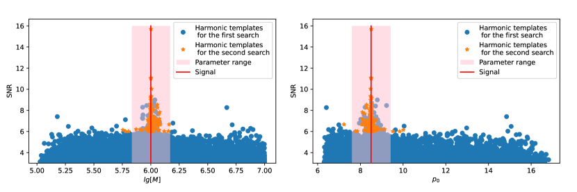
Figure 1: The distribution of the harmonic’s SNR for the parameters $M$ and $p_{0}$. We select only the strongest harmonic mode for each template. Templates with a high harmonic SNR cluster near the signal.

Next, we set the threshold value and boundaries for the search results to obtain the range of physical parameters. We select the top $\sim 0.01\,\%$ templates with the highest SNR corresponding to a SNR threshold of around 6. For the first search, we use approximately 500,000 templates. Among them are around 50,000 templates with ${\rm SNR}>3$ and only 80 templates with ${\rm SNR}>6$. We see in Fig. 1 that there are a few templates with ${\rm SNR}>6$ further away from the signal but most of the high SNR templates cluster around the signal. This phenomenon is particularly evident for the parameters $M$ and $p_{0}$. To obtain the boundaries for the physical parameters, we calculate the mean and standard deviation for the distribution of the templates. The mean value and the standard deviation for $\log_{10}(M/{\rm M_{\odot}})$ are $6.02$ and $0.29$, respectively, while the mean value and the standard deviation for $p_{0}$ are $8.75\,M$ and $1.52\,M$, respectively. We focus on the points locate in the boundaries $[\mu_{\theta}-\sigma_{\theta},\mu_{\theta}+\sigma_{\theta}]$, and update the parameters to $[5.73,6.31]$ and $[7.23,10.27]\,M$ for the ranges of $\log_{10}(M/{\rm M_{\odot}})$ and $p_{0}$, respectively.

The initial search provides a rough indication of the source parameter. We refine the search by performing a second round of search in the zoomed-in range. In the second round, we expand the boundaries obtained from the initial search by 10 %. For this search, we use approximately 100,000 templates, where we get 187 templates with a SNR greater than 6. We combine the results from this search and the previous search, and obtained a total of 267 templates with ${\rm SNR}>6$. The mean value and the standard deviation we get from the combined distribution for $\log_{10}(M/{\rm M_{\odot}})$ are $6.01$ and $0.16$, respectively, while the mean value and the standard deviation for $p_{0}$ are $8.58\,M$ and $0.90\,M$, respectively. Therefore, we obtain the final parameter range $[5.85,6.17]$ and $[7.68,9.48]\,M$ for $\log_{10}(M/{\rm M_{\odot}})$ and $p_{0}$, respectively.

In Fig. 1, results from the first coarse search are labeled in blue points and pink-shaded region. The orange stars represent the refined search round search results, and the injected value is indicated by the red vertical line. After the refined search, the denser templates allow us to increase the SNR threshold, which we used value of 7, to concentrate on better-fit templates. In the top left panel of Fig. 2, we present the phase evolution of the harmonics for all templates with ${\rm SNR}>7$, while the harmonics of the injected signal are represented with red dashed lines. We can clearly see that all templates with ${\rm SNR}>7$ have at least one harmonic whose phase evolution tracks the signal closely, and all phase evolutions display polynomial features.

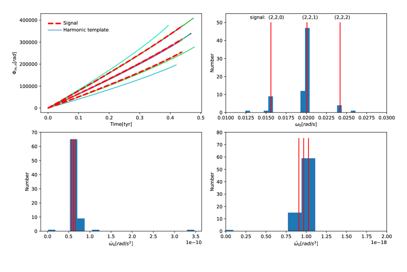
Figure 2: The phase evolution distribution of high SNR physical harmonic templates. The top-left panel illustrates the phase evolution for all high SNR templates.The remaining panels show the phenomenological parameter distributions of $\omega_{0}$, $\dot{\omega_{0}}$, and $\ddot{\omega_{0}}$ (c.f. Section III.2.1) in the initial time segment of $0.1\,{\rm yr}$, respectively.

III.2 Semi-coherent search with a phenomenological waveform

Using the physical waveforms to search is very time-consuming, especially considering the multi-peak nature. Hence we use a phenomenological waveform for the next search stage. The top left panel of Fig. 2 indicates that polynomial functions might be sufficient to describe the phase evolution. Here, a semi-coherent search is employed, where we divide the data into time segments of $0.1\,{\rm yr}$ and infer the phenomenological parameters for each time segment. Before discussing the details and results of the search in this stage, we introduce some basic concepts of the phenomenological waveforms we use in the following section.

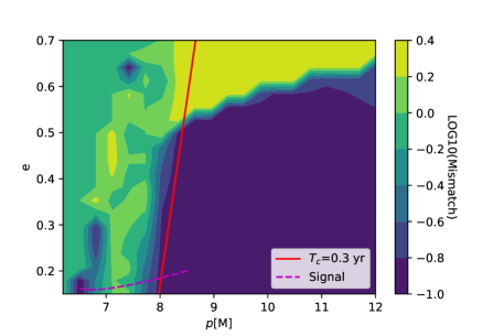
Figure 3: The mismatch between the phenomenological and physical waveforms with different $p$ and $e$. The purple dashed line indicates the $p-e$ evolution of the signal from (8.5,0.2) to (6.43, 0.165). The red solid line indicates where the evolution time from $(p,e)$ to the plunge is $0.3\,{\rm yr}$, points on the right side being longer than $0.3\,{\rm yr}$.

III.2.1 Phenomenological waveform

The key idea of searching for signals using a phenomenological waveform is that the evolution of the EMRI’s orbital frequency is relatively smooth in the early stage of the inspiral. In a short period, the phase $\Phi_{mn}(t)$ can be Taylor expanded as Wang et al. (2012b)

$$\Phi_{mn}(t)= \Phi_{mn}\left(t_{0}\right)+\omega_{m,n}\left(t_{0}\right)\left(t-t_{0}\right)+\frac{1}{2}\dot{\omega}_{m,n}\left(t_{0}\right)$$ (15)

$$\times\left(t-t_{0}\right)^{2}+\frac{1}{3}\ddot{\omega}_{m,n}\left(t_{0}\right)\left(t-t_{0}\right)^{3}+O(4),$$

where we define the angular frequency $\omega_{m,n}=:m\omega_{\phi}+n\omega_{r}$, and $\dot{\omega}_{m,n}$ and $\ddot{\omega}_{m,n}$ are its first and second time-derivatives, respectively. The amplitudes in GWs $A_{mn}$ evolve even smoother than the phase over an extended period of time. Moreover, detection is more sensitive to a mismatch in the phase than in the amplitude. Therefore, for simplicity, we ignore the time evolution of the amplitudes and treat all of them as constants Wang et al. (2012b); Hughes et al. (2021). The Doppler effect induced by the orbital motion of the detectors is also smoother than the phase over an extended time period and chance, we can also ignore it in the template.

To check the similarity of the phenomenological waveform to the physical waveform, we calculate their mismatch, which is defined as

$${\mathrm{M}ismatch}=1-\frac{(a\mid b)}{\sqrt{(a\mid a)(b\mid b)}},$$ (16)

where a and b are the phenomenological waveform and the physical waveform, respectively. The mismatch between the phenomenological and the physical waveforms for different orbital parameters $p$ and $e$ is shown in Fig. 3. Here, we consider a short time segment of $0.1\,{\rm yr}$ and fix other physical parameters, such as $M=10^{6}\,\rm M_{\odot}$, $\mu=10\,\rm M_{\odot}$. The dashed line indicates the $p-e$-evolution of the signal from (8.5,0.2) to (6.43, 0.165). The red solid line marks where the time from $(p,e)$ to plunge is $0.3\,{\rm yr}$, i.e., a source with parameters on the right side from the red line needs longer than $0.3\,{\rm yr}$ to plunge. We can observe that regions to the right side of the red line show good consistency between the phenomenological waveform and the physical waveform. Considering shorter time segments for the semi-coherent search can further increase the applicable range for phenomenological waveform Gair et al. (2004).

III.2.2 Template Search

At this stage, a semi-coherent approach is adopted to search with the phenomenological waveforms. Semi-coherent methods relax the stringent requirements on the phase accuracy of the models, combined with the usage of simpler waveforms like phenomenological waveforms for the search, the total computational time can be hugely compressed Gair et al. (2004). In exchange, the semi-coherent likelihood leads to wider posterior distributions, particularly on those parameters that strongly influence the phase of the GW signal. Semi-coherent methods are widely used in searches for continuous waves in LIGO/Virgo data Riles (2023); Prix and Shaltev (2012). Here, we divided the data into five segments, each with a duration of $0.1\,{\rm yr}$. Notice that the validity of the phenomlogical waveform drops significantly when the system approaches merge, in practise only the results from the first three segments were used.

In each segment, we search using three different harmonic modes of the phenomenological waveforms. We sample the posterior distribution of the phenomenological parameters for each harmonic mode within each segment. The posterior probability distribution of the parameters $p(\theta|d)$ can be obtained using a Bayesian analysis

$$p(\theta|d)=\frac{p(\theta)p(d|\theta)}{p(d)}$$ (17)

where $p(\theta)$ is the prior probability distribution of the parameters, $p(d|\theta)$ is the likelihood, and $p(d)$ is the evidence. The evidence is a normalization factor that is independent of the parameters and hence we can ignore it here. The standard Bayesian (log-)likelihood ratio function of the source parameters $\theta$, is given by

$$\Lambda(\theta):=(d|h)-\frac{1}{2}(h|h).$$ (18)

Next, we discuss how to select the prior for the parameters of a harmonic mode within each time segment. Based on the search results using physical waveforms in Section III.1, we can obtain harmonic phases that match the signal. We divide these phases into segments of $0.1\,{\rm yr}$ each and fit them using Eq. (15). The upper right and the two lower subplots in Fig. 2 show the distributions of the three phenomenological parameters $\omega_{0}$, $\dot{\omega}_{0}$, and $\ddot{\omega}_{0}$ for the harmonic phases in the first time segment, respectively. The distribution of $\omega_{0}$ shows three different harmonic modes. Despite the absence of evident harmonic structures in the parameter distributions of $\dot{\omega}_{0}$ and $\ddot{\omega}_{0}$, they can still provide a narrow parameter range. We summarize the prior parameter ranges of $\omega_{0}$, $\dot{\omega}_{0}$, and $\ddot{\omega}_{0}$ for the three main harmonic modes in the different time segments in Table 3. Furthermore, we refer to Table 2 for the selection of the priors for the extrinsic parameters.

Time segment	modes	$\omega_{0}$		$\dot{\omega}_{0}$		$\ddot{\omega}_{0}$
		prior	signal	prior	signal	prior	signal
1-segment	(2,0)	[0.015,0.017]	0.0158	[0,1e-10]	5.71e-11	[0,2e-18]	1.03e-18
	(2,1)	[0.019,0.021]	0.0201	[0,1e-10]	6.13e-11	[0,2e-18]	9.68e-19
	(2,2)	[0.024,0.026]	0.0244	[0,1e-10]	6.55e-11	[0,2e-18]	9.08e-19
2-segment	(2,0)	[0.016,0.018]	0.0166	[0,1e-10]	7.11e-11	[0,3e-18]	1.73e-18
	(2,1)	[0.020,0.022]	0.021	[0,1e-10]	7.46e-11	[0,3e-18]	1.56e-18
	(2,2)	[0.024,0.026]	0.0253	[0,1e-10]	7.80e-11	[0,3e-18]	1.39e-18
3-segment	(2,0)	[0.016,0.018]	0.0177	[-1e-10,1e-10]	9.32e-11	[0,1e-16]	3.57e-18
	(2,1)	[0.019,0.024]	0.022	[-1e-10,1e-10]	9.49e-11	[0,1e-16]	3.01e-18
	(2,2)	[0.023,0.027]	0.026	[-1e-10,1e-10]	9.66e-11	[0,1e-16]	2.46e-18

Table 3: The prior distributions for the three phenomenological parameters $\omega_{0}$, $\dot{\omega}_{0}$, and $\ddot{\omega}_{0}$ in the different time segments.

III.2.3 Results of the phenomenological waveform search

For this search, we employ nested sampling to obtain the posterior distribution for each harmonic mode and each time segment to extensively explore the high posterior regions Skilling (2004); Speagle (2020). In addition to estimating the posterior distribution, nested sampling methods also can calculate the evidence by integrating the prior within nested ‘shells’ of a constant likelihood. In practice, for each nested sampling execution, we use approximately $500$ core hours before stop the sampling.

We execute a total of 11 nested sampling operations. The results of nested sampling for each harmonic mode and each time segment are summarized in Table 4. The results show the median and the 1-$\sigma$ range of the posterior distribution for the phenomenological parameters. We see that the bias of $\omega_{0}$ is less than the bias of $\dot{\omega}_{0}$, and the bias of $\dot{\omega}_{0}$ is smaller than the bias of $\ddot{\omega}_{0}$. This can be understood as the lower order term in the Taylor expansion of the phase evolution can be better tracked. In the first two time segments, the bias precision for $\omega_{0}$ is $\sim 0.1\,\%$, and it can even reach $10^{-6}$. Furthermore, the bias precision for the parameter $\dot{\omega}_{0}$ also remains within 10 %. However, as the observation time segments get closer to the plunge, the measured bias of the phenomenological parameters increases because the orbital evolution of the signal becomes faster, leading to the failure of the phenomenological waveform reproducing the signal accurately.

As an illustration, we display the results of the posterior distribution sampling for the phenomenological parameters of the $(2,0)$ harmonic mode for the first time segment in Fig. 4. We see that the posterior distributions for the parameters $\omega$ and $\dot{\omega}$ exhibit very narrow and sharp peaks. The 1-$\sigma$ ranges for $\omega$ and $\dot{\omega}$ are 0.01 % and 1 % of the prior range, respectively while the 1-$\sigma$ range for $\ddot{\omega}$ can extend to 10 % of the prior range. However, for extrinsic parameters like the initial phase $\Phi_{0}$ and the positional parameters ($\theta,\phi,\psi$), the measurements are not accurate. This is because we do not take into account the evolution of the amplitude over time and the mutual coupling between these extrinsic parameters, causing the measurement results to deviate from the true values.

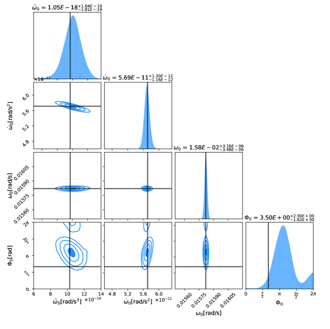
Figure 4: The posterior distribution of the four phenomenological parameters for the first time segment (2,0) mode.

1-segment	mode(m,n)	(2,0)			(2,1)			(2,2)
	parameters	$\omega_{0}/10^{-2}[rad/s]$	$\dot{\omega}_{0}/10^{-11}[rad/s^{2}]$	$\ddot{\omega}_{0}/10^{-18}[rad/s^{3}]$	$\omega_{0}/10^{-2}[rad/s]$	$\dot{\omega}_{0}/10^{-11}[rad/s^{2}]$	$\ddot{\omega}_{0}/10^{-18}[rad/s^{3}]$	$\omega_{0}/10^{-2}[rad/s]$	$\dot{\omega}_{0}/10^{-11}[rad/s^{2}]$	$\ddot{\omega}_{0}/10^{-18}[rad/s^{3}]$
	signal	1.58	5.71	1.03	2.01	6.13	0.97	2.44	6.55	0.91
	measurement	$1.58_{-3.48E-4}^{+3.16E-4}$	$5.69_{-1.16E-1}^{+1.30E-1}$	$1.05_{-1.81E-1}^{+1.64E-1}$	$2.01_{-2.24E-4}^{+2.15E-4}$	$6.15_{-7.70E-2}^{+8.05E-2}$	$0.95_{-1.10E-1}^{+1.07E-1}$	$2.43_{-2.57E-4}^{+2.68E-4}$	$6.43_{-9.56E-2}^{+9.23E-2}$	$1.09_{-1.25E-1}^{+1.31E-1}$
	Bias	0.00%	0.30 %	2.37%	0.00%	0.26%	1.76%	0.31%	1.82%	19.72%
2-segment	mode(m,n)	(2,0)			(2,1)			(2,2)
	parameters	$\frac{\omega_{0}}{10^{-2}}$	$\frac{\dot{\omega}_{0}}{10^{-10}}$	$\frac{\ddot{\omega}_{0}}{10^{-18}}$	$\frac{\omega_{0}}{10^{-2}}$	$\frac{\dot{\omega}_{0}}{10^{-10}}$	$\frac{\ddot{\omega}_{0}}{10^{-18}}$	$\frac{\omega_{0}}{10^{-2}}$	$\frac{\dot{\omega}_{0}}{10^{-10}}$	$\frac{\ddot{\omega}_{0}}{10^{-18}}$
	signal	1.66	7.11	1.73	2.10	7.46	1.56	2.53	7.80	1.39
	measurement	$1.66_{-8.08E-3}^{+3.68E-4}$	$7.10_{-1.35E-1}^{+1.12E-1}$	$1.72_{-1.57E-1}^{+1.85E-1}$	$2.10_{-3.05E-4}^{+1.27E-3}$	$6.86_{-3.11E-1}^{+1.09E-1}$	$2.18_{-1.46E-1}^{+3.24E-1}$	$2.54_{-1.84E-4}^{+1.97E-4}$	$7.50_{-7.94E-2}^{+7.32E-2}$	$1.59_{-1.06E-1}^{+1.12E-1}$
	Bias	0.00%	0.13%	6.54%	0.11%	7.99%	39.80%	0.48 %	3.96%	14.5%
3-segment	mode(m,n)	(2,0)			(2,1)			(2,2)
	parameters	$\frac{\omega_{0}}{10^{-2}}$	$\frac{\dot{\omega}_{0}}{10^{-10}}$	$\frac{\ddot{\omega}_{0}}{10^{-18}}$	$\frac{\omega_{0}}{10^{-2}}$	$\frac{\dot{\omega}_{0}}{10^{-10}}$	$\frac{\ddot{\omega}_{0}}{10^{-18}}$	$\frac{\omega_{0}}{10^{-2}}$	$\frac{\dot{\omega}_{0}}{10^{-10}}$	$\frac{\ddot{\omega}_{0}}{10^{-18}}$
	signal	1.77	9.32	3.57	2.20	9.49	3.01	2.64	9.66	2.46
	measurement	$1.68_{-6.17E-2}^{+1.03E-1}$	$7.54_{-11.7}^{+2.22}$	$26.4_{-}21.2^{+36.5}$	$1.94_{-1.44E-1}^{+3.64E-1}$	$3.24_{-7.76}^{+5.29}$	$17.5_{-15.2}^{+48.0}$	$2.40_{-9.56E-2}^{+2.37E-1}$	$1.81_{-6.04}^{+6.51}$	$19.6_{-13.6}^{+34.3}$
	Bias	5.09%	19.17%	637.71%	11.74%	65.84%	480.89%	9.05%	87.33%	699.28%

Table 4: The measurement results of phenomenological parameters ($\omega_{0},\dot{\omega}_{0},\ddot{\omega}_{0}$) with different harmonics for different time segments.

III.3 Hierarchical search for physical parameters

Achieving the data analysis of EMRI signals without extensive prior knowledge of the physical parameters poses a formidable challenge since expanding the parameter space for the search entails a commensurate increase in computational demands. For example, in previous works the parameter range for $\log_{10}(M/{\rm M_{\odot}})$ was within $\sim 0.05$ for a harmonic search Babak et al. (2009a), it was within $\sim 0.2$ when using a MCMC method Chua and Cutler (2022), and for a phenomenological search $M$ was fixed Wang et al. (2012a). In this study, we combined various search methods to perform a hierarchical search for the physical parameters considering a parameter range for $M$ over two orders of magnitudes.

Our ultimate goal is to obtain the range for the physical parameters using a hierarchical search method based on the highly precise measurement results of the phenomenological parameters in Section III.2 and the rough range of physical parameters obtained in Section III.1. The phenomenological parameters of different harmonics at various time segments provide strong constraints on the physical parameters and thus we attempt to map the posterior distribution of the phenomenological parameters to the physical parameters.

III.3.1 Search method

It is difficult to directly convert from phenomenological waveform parameters to physical parameters. On the one hand, there is no analytical formula to deduce the physical parameters directly from the phenomenological parameters. On the other hand, the multi-peak structure of the posterior distribution of physical parameters means that it might be one-to-many mapping from phenomenological parameters.

Here, we employ a grid-based approach to the physical parameters to facilitate the resolution of this procedure. For each point on the grid, we use FEW to calculate the harmonic phase evolution for each time segment. Then, we fit them using Eq. 15 to obtain the corresponding phenomenological parameters. In the Schwarzschild eccentricity condition, the parameters $[M,\mu,p_{0},e_{0}]$ directly determine the trajectory of the phase evolution. Therefore, the set of four physical parameters can be transformed into the phenomenological parameter space. Here, we choose 18 phenomenological parameters for the first two time segments with three main harmonic modes in each segment and the three parameters ($\omega_{0},\dot{\omega}_{0},\ddot{\omega}_{0}$) for each harmonic mode. This choice is based on the exceptional accuracy of the parameter measurement in these segments when compared to the other time segments (see Table 4). Moreover, we further choose a set of nine phenomenological parameters, which include the $(2,0)$ and $(2,1)$ modes for the first time segment and the $(2,0)$ mode for the second time segment, which are the closest to the signal in terms of their corresponding phenomenological parameters and will be used for a finer differentiation in the search.

For each phenomenological parameter, we check if the parameter falls within the 3-$\sigma$ posterior distribution obtained from the nested sampling. In principle, one can depict the physical parameters using a sufficiently dense grid. The number of such “close” parameters is used to rank the fitness. However, to account for practical computational constraints we first employ a coarse grid to the region of the parameter space obtained from the harmonic mode search and then a finer grid to a smaller region identified during the search with the coarse grid.

III.3.2 Results of the hierarchical search

Fig. 5 shows the hierarchical research of physical parameters, showcasing the outcomes at each stage of the search process. The left image represents the search results obtained from the physical harmonic search. The middle and right images depict the outcomes obtained through coarse and fine grid-based methods, respectively.

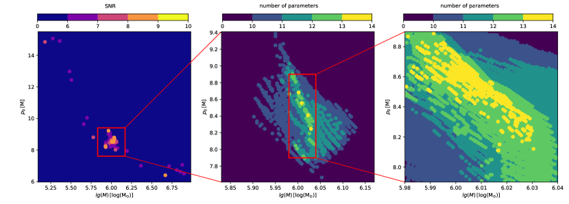
Figure 5: The results of the hierarchical search for physical parameters. The left graph shows the search result using the physical harmonic waveforms. The middle graph presents the search results from the coarse grid and the results from the fine grid search are shown in the right graph. Different search methods and strategies were employed here, as detailed in Sections III.1 and III.3.

From the distribution of parameters from the harmonic template search introduced in Section III.1, we obtain the parameter range ($[5.85,6.17]$ for $\log_{10}(M/{\rm M_{\odot}})$ and $[7.68,9.48]\,M$ for $p_{0}$) shown in the red box in the left graph of Fig. 5. For the grid-based search, the parameter range is determined based on the number of parameters for which the phenomenological parameters fall within the 3-$\sigma$ posterior distribution obtained in Section III.2. This is not equivalent to the criteria in the first step.

For the coarse grid, we uniformly sample 100 points for the parameters $M$ and $p_{0}$ within the range of the first step results. Additionally, for the parameters $e_{0}$ and $\mu$, we uniformly sample 10 points within the parameter ranges $[0,0.7]$ and $[5,15]{\mathrm{M}_{\odot}}$, respectively. This grid comprises a total of 1,000,000 points and the overall computational cost amounts to approximately 500 core hours. In this grid, 94 best-fit grid points, each contains 12 phenomenological parameters that fall within the 3-$\sigma$ range, are shown in the center graph of Fig. 5. These phenomenological parameters correspond to the range of physical parameters $\log_{10}(M/{\mathrm{M}_{\odot}})\in[5.98,6.04]$, $p_{0}\in[7.9,8.9]M$, $e_{0}\in[0,0.4]$, and $\mu\in[8,13]{\mathrm{M}_{\odot}}$ and are shown as gray stars in Fig. 6.

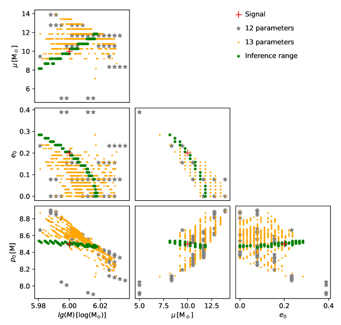
Figure 6: The hierarchical search results for the four physical parameters obtained from the coarse grid and the fine grid. The terms ’12 parameters’ and ’13 parameters’ refer to the presence of 12 phenomenological parameters within the 3-$\sigma$ range of the coarse grid and 13 phenomenological parameters within the 3-$\sigma$ range of the fine grid, respectively. The inference range indicates that a specific set of nine parameters that were measured with particularly high precision falls within the 3-$\sigma$ range.

For the fine grid, the grid parameters’ range is based on the results of the coarse grid. Similarly to the previous search, we uniformly sample 100 points for the parameters $M$ and $p_{0}$, and 10 points for $e_{0}$ but 50 points for $\mu$. Using this grid, we find 807 grid points corresponding to 13 phenomenological parameters falling within the 3-$\sigma$ range. These points are shown as yellow points in Fig. 6. Despite having 14 parameters falling within the 3-$\sigma$ range here, many templates constitute random combinations of the 18 parameters. However, among these 18 parameters, several are significantly biased, with a bias of up to 40% from the signal. Therefore, as a followup search, we use the nine parameters that are measured with high accuracy (see Section III.3.1), and we require that all of them must fall within the 3-$\sigma$ range. The grid points fulfilling this additional condition are shown as green points in Fig. 6. We can see that there is a strong correlation among these physical parameters and that they always contain the signal. This is due to the presence of different harmonics and segmented phase evolution information, which inherently imposes strong constraints on the physical parameters themselves. In the end, we constrain the range of physical parameters to $[5.980,6.018]$ for $\log_{10}(M/{\rm M_{\odot}})$, $[8.455,8.535]\,M$ for $p_{0}$, $[0,0.284]$ for $e_{0}$, and $[8.158,11.842]\,{\rm M_{\odot}}$ for $\mu$.

Based on high-precision measurements of the phenomenological parameters and the physical parameter ranges obtained from the search results of the physical waveforms, we achieve the relative error in the measurement of $M$ to be within 4 % while the smallest errors for the other parameters can be within 0.5 %. This parameter accuracy is sufficient for the requirement of future EMRI parameter inference Chua and Cutler (2021).

IV conclusions and disscusion

Accomplishing the identification of EMRI signals and providing ranges for the physical parameters for subsequent parameter inference is challenging. On the one hand, performing searches using only physical waveforms encounters difficulties due to the multi-peak structure of the posterior distribution of physical parameters which makes it difficult for stochastic sampling algorithms to navigate between peaks. Even employing something like the “one-step” likelihood function approach does not provide global guidance for the region of the high posterior regions. On the other hand, when only employing phenomenological waveforms for the searches, the lack of prior information about phenomenological and physical parameters makes signal searching and the inference of physical parameters difficult. Therefore, we adopt in this work a combined approach of both methods. Phenomenological waveform searches effectively avoid the multi-peak structure of the posterior distribution of physical parameters, while physical parameter searches provide prior information to narrow down the search space of parameters.

We have achieved for the first time the identification of EMRI signals without any additional prior information on physical parameters. High-precision measurements of EMRI signals have been achieved using a hierarchical search that combines the search for physical parameters that guides subsequent parameter inference and a semi-coherent search with phenomenological waveforms that reaches precision levels down to $10^{-4}$ for the phenomenological waveform parameters $\omega_{0}$, $\dot{\omega}_{0}$, and $\ddot{\omega}_{0}$. As a result, we obtain measurement relative errors of less than 4 % for the mass of the MBH, while keeping the relative errors of the other parameters within as small as 0.5 %.

Although we only search for an EMRI signal assuming a Schwarzschild eccentric background, we believe the method presented can be used universally for the search of EMRI signals for several reasons:

• In Ref. Babak et al. (2009b) the applicability of the harmonic detection in AK waveforms under the Kerr eccentric background was demonstrated. Once a sufficient number of harmonic templates match the signal, a physical parameter range can be established. Our objective in this step is not only to obtain the range of physical parameters but also to precisely extract the phase evolution information. Furthermore, we employ the more accurate fully relativistic FEW waveforms to obtain a more realistic phase evolution.

• In Ref. Wang et al. (2012b), the amplitude evolution was also neglected, and an expansion of the phase as a Taylor series of third order was also used. Our goal in this step was not only to achieve the matching for phase of the signal but, more importantly, to achieve high-precision measurements of phenomenological parameters which is crucial for the hierarchical search of the physical parameters.

• The difference between the Schwarzschild background and the Kerr background induces a relatively slow difference in the frequency evolution in the early inspiral phase of the EMRI signal. In Fig.3, the mismatch between the phenomenological and physical waveforms implies that there can be a high level of correlation during the early inspiral phase of the EMRI signal. Therefore, within a short time segment, the signal can be well-matched using the phenomenological waveform. In addition, FEW interpolates cubic splines of sparse phases to obtain complete phase evolution Chua et al. (2021); Katz et al. (2021). The farther away from the plunge in time, the sparser the phase evolution is calculated. Hence, fitting the phase within shorter time segments at earlier stages yields improved fitting outcomes.

In the future, more complex scenarios to approach the final EMRI signal processing pipeline should be studied. For example, the application of fully relativistic Kerr waveforms for the identification should be explored as well as investigating the more intricate Time Delay Interference response. Moreover, the high-precision measurements based on phenomenological parameters could also be used for the spatial localization of EMRI events. The effectivity of converting the phenomenological waveform parameters into physical parameters in this case should be studied in more detail.

References

- Abbott et al. (2019) B. P. Abbott et al. (LIGO Scientific, Virgo), Phys. Rev. X 9, 031040 (2019), arXiv:1811.12907 [astro-ph.HE] .
- Abbott et al. (2020) R. Abbott et al. (LIGO Scientific, Virgo), (2020), arXiv:2010.14527 [gr-qc] .
- Abbott et al. (2021) R. Abbott et al. (LIGO Scientific, VIRGO, KAGRA), (2021), arXiv:2111.03606 [gr-qc] .
- Danzmann and Rüdiger (2003) K. Danzmann and A. Rüdiger, Classical and Quantum Gravity 20, S1 (2003).
- Amaro-Seoane et al. (2013) P. Amaro-Seoane et al., GW Notes 6, 4 (2013), arXiv:1201.3621 [astro-ph.CO] .
- Amaro-Seoane et al. (2017) P. Amaro-Seoane et al. (LISA), (2017), arXiv:1702.00786 [astro-ph.IM] .
- Mei et al. (2020) J. Mei, Y.-Z. Bai, J. Bao, E. Barausse, L. Cai, E. Canuto, B. Cao, W.-M. Chen, Y. Chen, Y.-W. Ding, et al., Progress of Theoretical and Experimental Physics (2020).
- Torres-Orjuela et al. (2023) A. Torres-Orjuela, S.-J. Huang, Z.-C. Liang, S. Liu, H.-T. Wang, C.-Q. Ye, Y.-M. Hu, and J. Mei, arXiv e-prints , arXiv:2307.16628 (2023), arXiv:2307.16628 [gr-qc] .
- Amaro-Seoane et al. (2007) P. Amaro-Seoane, J. R. Gair, M. Freitag, M. Coleman Miller, I. Mandel, C. J. Cutler, and S. Babak, Class. Quant. Grav. 24, R113 (2007), arXiv:astro-ph/0703495 .
- Amaro-Seoane (2018) P. Amaro-Seoane, Living Rev. Rel. 21, 4 (2018), arXiv:1205.5240 [astro-ph.CO] .
- Babak et al. (2017) S. Babak, J. Gair, A. Sesana, E. Barausse, C. F. Sopuerta, C. P. Berry, E. Berti, P. Amaro-Seoane, A. Petiteau, and A. Klein, Physical Review D 95, 103012 (2017).
- Gair et al. (2017) J. R. Gair, S. Babak, A. Sesana, P. Amaro-Seoane, E. Barausse, C. P. Berry, E. Berti, and C. Sopuerta, in Journal of Physics: Conference Series, Vol. 840 (IOP Publishing, 2017) p. 012021.
- Fan et al. (2020) H.-M. Fan, Y.-M. Hu, E. Barausse, A. Sesana, J.-d. Zhang, X. Zhang, T.-G. Zi, J. Mei, et al., Physical Review D 102, 063016 (2020).
- Zi et al. (2021) T.-G. Zi, J.-D. Zhang, H.-M. Fan, X.-T. Zhang, Y.-M. Hu, C. Shi, and J. Mei, Phys. Rev. D 104, 064008 (2021), arXiv:2104.06047 [gr-qc] .
- Maselli et al. (2022) A. Maselli, N. Franchini, L. Gualtieri, T. P. Sotiriou, S. Barsanti, and P. Pani, Nature Astron. 6, 464 (2022), arXiv:2106.11325 [gr-qc] .
- Barsanti et al. (2022) S. Barsanti, N. Franchini, L. Gualtieri, A. Maselli, and T. P. Sotiriou, “Extreme mass-ratio inspirals as probes of scalar fields: eccentric equatorial orbits around Kerr black holes,” (2022), arXiv:2203.05003 [gr-qc] .
- Torres-Orjuela et al. (2021) A. Torres-Orjuela, P. A. Seoane, Z. Xuan, A. J. Chua, M. J. Rosell, and X. Chen, Physical Review Letters 127, 041102 (2021).
- Barausse and Rezzolla (2008) E. Barausse and L. Rezzolla, Phys. Rev. D 77, 104027 (2008), arXiv:0711.4558 [gr-qc] .
- Pan et al. (2021) Z. Pan, Z. Lyu, and H. Yang, Phys. Rev. D 104, 063007 (2021), arXiv:2104.01208 [astro-ph.HE] .
- Fan et al. (2022) H.-M. Fan, S. Zhong, Z.-C. Liang, Z. Wu, J.-d. Zhang, and Y.-M. Hu, Phys. Rev. D 106, 124028 (2022), arXiv:2209.13387 [gr-qc] .
- Yunes et al. (2011) N. Yunes, B. Kocsis, A. Loeb, and Z. Haiman, Phys. Rev. Lett. 107, 171103 (2011).
- Barausse et al. (2015) E. Barausse, V. Cardoso, and P. Pani, in Journal of Physics Conference Series, Journal of Physics Conference Series, Vol. 610 (2015) p. 12044.
- Cardoso et al. (2022) V. Cardoso, K. Destounis, F. Duque, R. P. Macedo, and A. Maselli, Physical Review Letters 129, 241103 (2022).
- Gair et al. (2010) J. R. Gair, C. Tang, and M. Volonteri, Phys. Rev. D 81, 104014 (2010).
- MacLeod and Hogan (2008) C. L. MacLeod and C. J. Hogan, Phys. Rev. D 77, 043512 (2008), arXiv:0712.0618 [astro-ph] .
- Laghi et al. (2021) D. Laghi, N. Tamanini, W. Del Pozzo, A. Sesana, J. Gair, and S. Babak, arXiv e-prints , arXiv:2102.01708 (2021), arXiv:2102.01708 [astro-ph.CO] .
- Hughes et al. (2005) S. A. Hughes, S. Drasco, E. E. Flanagan, and J. Franklin, Physical review letters 94, 221101 (2005).
- van de Meent (2018) M. van de Meent, Phys. Rev. D 97, 104033 (2018).
- Barack (2009) L. Barack, Class. Quant. Grav. 26, 213001 (2009), arXiv:0908.1664 [gr-qc] .
- Barack and Cutler (2004) L. Barack and C. Cutler, Phys. Rev. D 69, 082005 (2004), arXiv:gr-qc/0310125 [gr-qc] .
- Babak et al. (2007) S. Babak, H. Fang, J. R. Gair, K. Glampedakis, and S. A. Hughes, Phys. Rev. D 75, 024005 (2007).
- Chua et al. (2017) A. J. Chua, C. J. Moore, and J. R. Gair, Physical Review D 96, 044005 (2017).
- Chua et al. (2021) A. J. Chua, M. L. Katz, N. Warburton, and S. A. Hughes, Physical Review Letters 126, 051102 (2021).
- Katz et al. (2021) M. L. Katz, A. J. Chua, L. Speri, N. Warburton, and S. A. Hughes, Physical Review D 104, 064047 (2021).
- Chua and Cutler (2022) A. J. Chua and C. J. Cutler, Physical Review D 106, 124046 (2022).
- Gair et al. (2004) J. R. Gair, L. Barack, T. Creighton, C. Cutler, S. L. Larson, E. S. Phinney, and M. Vallisneri, Classical and Quantum Gravity 21, S1595 (2004).
- Chua (2022) A. J. Chua, Physical Review D 106, 104051 (2022).
- Zhang et al. (2022) X.-T. Zhang, C. Messenger, N. Korsakova, M. L. Chan, Y.-M. Hu, and J.-d. Zhang, Physical Review D 105, 123027 (2022).
- Wang et al. (2012a) Y. Wang, Y. Shang, S. Babak, Y. Shang, and S. Babak, Phys. Rev. D 86, 104050 (2012a), arXiv:1207.4956 [gr-qc] .
- Babak et al. (2009a) S. Babak, J. R. Gair, and E. K. Porter, Classical and quantum gravity 26, 135004 (2009a).
- Wang et al. (2015) Y. Wang, G. Heinzel, and K. Danzmann, Physical Review D 92, 044037 (2015).
- Gair and Wen (2005) J. Gair and L. Wen, Classical and Quantum Gravity 22, S1359 (2005).
- Wen and Gair (2005) L. Wen and J. R. Gair, Classical and Quantum Gravity 22, S445 (2005).
- Gair et al. (2008a) J. R. Gair, I. Mandel, and L. Wen, Class. Quant. Grav. 25, 184031 (2008a), arXiv:0804.1084 [gr-qc] .
- Gair et al. (2008b) J. R. Gair, E. Porter, S. Babak, and L. Barack, Classical and Quantum Gravity 25, 184030 (2008b).
- Chua (2016) A. J. K. Chua, J. Phys. Conf. Ser. 716, 012028 (2016), arXiv:1602.00620 [gr-qc] .
- Chua et al. (2020) A. J. K. Chua, N. Korsakova, C. J. Moore, J. R. Gair, and S. Babak, Phys. Rev. D 101, 044027 (2020), arXiv:1912.11543 [astro-ph.IM] .
- Chua and Cutler (2021) A. J. Chua and C. J. Cutler, arXiv preprint arXiv:2109.14254 (2021).
- Arnaud et al. (2007) K. A. Arnaud, G. Auger, S. Babak, J. G. Baker, M. J. Benacquista, E. Bloomer, D. A. Brown, J. B. Camp, J. K. Cannizzo, N. Christensen, J. Clark, N. J. Cornish, J. Crowder, C. Cutler, L. S. Finn, H. Halloin, K. Hayama, M. Hendry, O. Jeannin, A. Królak, S. L. Larson, I. Mandel, C. Messenger, R. Meyer, S. Mohanty, R. Nayak, K. Numata, A. Petiteau, M. Pitkin, E. Plagnol, E. K. Porter, R. Prix, C. Roever, A. Stroeer, R. Thirumalainambi, D. E. Thompson, J. Toher, R. Umstaetter, M. Vallisneri, A. Vecchio, J. Veitch, J.-Y. Vinet, J. T. Whelan, and G. Woan, Classical and Quantum Gravity 24, S529 (2007).
- Babak et al. (2008) S. Babak et al., Class. Quant. Grav. 25, 184026 (2008), arXiv:0806.2110 [gr-qc] .
- Babak et al. (2010) S. Babak et al. (Mock LISA Data Challenge Task Force), Class. Quant. Grav. 27, 084009 (2010), arXiv:0912.0548 [gr-qc] .
- Amaro-Seoane et al. (2011) P. Amaro-Seoane, B. Schutz, and J. Thornburg, arXiv preprint arXiv:1102.3647 (2011).
- Chua and Gair (2015) A. J. K. Chua and J. R. Gair, Classical and Quantum Gravity 32, 232002 (2015).
- Osburn et al. (2016) T. Osburn, N. Warburton, and C. R. Evans, Physical Review D 93, 064024 (2016).
- Van De Meent (2018) M. Van De Meent, Physical Review D 97, 104033 (2018).
- Hughes et al. (2021) S. A. Hughes, N. Warburton, G. Khanna, A. J. Chua, and M. L. Katz, Physical Review D 103, 104014 (2021).
- Chua et al. (2019) A. J. Chua, C. R. Galley, and M. Vallisneri, Physical review letters 122, 211101 (2019).
- Luo et al. (2016a) J. Luo, L.-S. Chen, H.-Z. Duan, Y.-G. Gong, S. Hu, J. Ji, Q. Liu, J. Mei, V. Milyukov, M. Sazhin, et al., Classical and Quantum Gravity 33, 035010 (2016a).
- Hu et al. (2018) X.-C. Hu, X.-H. Li, Y. Wang, W.-F. Feng, M.-Y. Zhou, Y.-M. Hu, S.-C. Hu, J.-W. Mei, and C.-G. Shao, Class. Quant. Grav. 35, 095008 (2018), arXiv:1803.03368 [gr-qc] .
- Luo et al. (2016b) J. Luo et al. (TianQin), Class. Quant. Grav. 33, 035010 (2016b), arXiv:1512.02076 [astro-ph.IM] .
- Liu et al. (2020) S. Liu, Y.-M. Hu, J.-d. Zhang, J. Mei, et al., Physical Review D 101, 103027 (2020).
- Babak (2008) S. Babak, Classical and Quantum Gravity 25, 195011 (2008).
- Babak et al. (2009b) S. Babak, J. R. Gair, and E. K. Porter, Classical and quantum gravity 26, 135004 (2009b).
- Wang et al. (2012b) Y. Wang, Y. Shang, and S. Babak, Physical Review D 86, 104050 (2012b).
- Riles (2023) K. Riles, Living Reviews in Relativity 26, 3 (2023).
- Prix and Shaltev (2012) R. Prix and M. Shaltev, Physical Review D 85, 084010 (2012).
- Skilling (2004) J. Skilling, in Aip conference proceedings, Vol. 735 (American Institute of Physics, 2004) pp. 395–405.
- Speagle (2020) J. S. Speagle, Monthly Notices of the Royal Astronomical Society 493, 3132 (2020).
- van der Walt et al. (2011) S. van der Walt, S. C. Colbert, and G. Varoquaux, Comput. Sci. Eng. 13, 22 (2011), arXiv:1102.1523 [cs.MS] .
- Virtanen et al. (2020) P. Virtanen et al., Nature Meth. 17, 261 (2020), arXiv:1907.10121 [cs.MS] .
- Hunter (2007) J. D. Hunter, Comput. Sci. Eng. 9, 90 (2007).