High-dimensional Bayesian Optimization
with Group Testing

Abstract

Bayesian optimization is an effective method for optimizing expensive-to-evaluate black-box functions. High-dimensional problems are particularly challenging as the surrogate model of the objective suffers from the curse of dimensionality, which makes accurate modeling difficult. We propose a group testing approach to identify active variables to facilitate efficient optimization in these domains. The proposed algorithm, Group Testing Bayesian Optimization (GTBO), first runs a testing phase where groups of variables are systematically selected and tested on whether they influence the objective. To that end, we extend the well-established theory of group testing to functions of continuous ranges. In the second phase, GTBO guides optimization by placing more importance on the active dimensions. By exploiting the axis-aligned subspace assumption, GTBO is competitive against state-of-the-art methods on several synthetic and real-world high-dimensional optimization tasks. Furthermore, GTBO aids in the discovery of active parameters in applications, thereby enhancing practitioners’ understanding of the problem at hand.

1 Introduction

Noisy and expensive-to-evaluate black-box functions occur in many practical optimization tasks, including material design (Zhang et al., 2020), hardware design (Nardi et al., 2019; Ejjeh et al., 2022), hyperparameter tuning (Kandasamy et al., 2018; Ru et al., 2020; Chen et al., 2018; Hvarfner et al., 2022), and robotics (Calandra et al., 2014; Berkenkamp et al., 2021; Mayr et al., 2022). Bayesian Optimization (BO) is an established framework that allows the optimization of such problems in a sample-efficient manner (Shahriari et al., 2016; Frazier, 2018). While BO is a popular approach for black-box optimization problems, its susceptibility to the curse of dimensionality has impaired its applicability to high-dimensional problems, such as in robotics (Calandra et al., 2014), joint neural architecture search and hyperparameter optimization (Bansal et al., 2022), drug discovery (Negoescu et al., 2011), chemical engineering (Burger et al., 2020), and vehicle design (Jones, 2008).

In recent years, efficient approaches have been proposed to tackle the limitations of BO in high dimensions. Many of these approaches assume the existence of a low-dimensional active subspace of the input domain that has a significantly larger impact on the optimization objective than its complement (Wang et al., 2016; Letham et al., 2020). In many applications, the active subspace is further assumed to be axis-aligned (Nayebi et al., 2019; Eriksson and Jankowiak, 2021; Papenmeier et al., 2022, 2023), i.e., only a set of all considered variables impact the objective. The assumption of axis-aligned subspaces is foundational for many successful approaches (Nayebi et al., 2019; Eriksson and Jankowiak, 2021; Song et al., 2022). While it is assumed to hold true for many practical problems, such as in engineering or hyperparameter tuning, few approaches use it to its full extent: either they rely on random embeddings that need to be higher-dimensional than the active subspace to have a high probability of containing the optimum (Nayebi et al., 2019; Papenmeier et al., 2022), or they carry out the optimization in the full-dimensional space while disregarding some of the dimensions dynamically (Eriksson and Jankowiak, 2021; Hvarfner et al., 2023; Song et al., 2022).

Knowing the active dimensions of a problem yields additional insight into the application, allowing the user to decide which problem parameters deserve more attention in the future. When the active subspace is axis-aligned, finding the active dimensions can be framed as a feature selection problem. A straightforward approach is first to learn the active dimensions using a dedicated feature selection approach and subsequently optimize over the learned subspace. We propose to initially find the active dimensions using an information-theoretic approach built around the well-established theory of group testing (Dorfman, 1943). Group testing is the problem of finding several active elements within a larger set by iteratively testing groups of elements to distinguish active members. We develop the theory needed to transition noisy group testing, which otherwise only allows binary observations, to work with evaluations of continuous black-box functions. This enables group testing in BO and other applications, such as feature selection for regression problems. The contribution of this work is:

1. We extend the theory of group testing to feature importance analysis in a continuous setting tailored towards Gaussian process modeling.

2. We introduce Group Testing Bayesian Optimization (GTBO), a novel BO method that finds active variables by testing groups of variables using a mutual information criterion.

3. We demonstrate that GTBO frequently outperforms state-of-the-art high-dimensional methods and reliably identifies active dimensions with high probability when the underlying assumptions hold.

2 Background

2.1 High-dimensional Bayesian optimization

We aim to find a minimizer $\bm{x}^{*}\in\operatorname*{arg\,min}_{\bm{x}\in\mathcal{X}}f(\bm{x})$ of the black-box function $f(\bm{x}):\mathcal{X}\rightarrow\mathbb{R}$, over the $D$-dimensional input space $\mathcal{X}=[0,1]^{D}$. We assume that $f$ can only be observed point-wise and that the observation is perturbed by noise, $y(\bm{x})=f(\bm{x})+\varepsilon_{i}$ with $\varepsilon_{i}\sim\mathcal{N}(0,\sigma_{n}^{2})$, where $\sigma_{n}^{2}$ is the noise variance. We further assume $f$ to be expensive to evaluate, such that the number of function evaluations is limited. In this work, we consider problems of high dimensionality $D$, where only $d_{e}$ dimensions are active, and the other ${D-d_{e}}$ dimensions are inactive. Here, inactive means that the function value changes only marginally along the inactive dimensions in relation to the active dimensions to the extent that satisfactory optimization performance can be obtained by considering the active dimensions alone. The assumption of active and inactive dimensions is equivalent to assuming an axis-aligned active subspace (Eriksson and Jankowiak, 2021), i.e., a subspace that can be obtained by removing the inactive dimensions. We refer the reader to Frazier (2018) for an in-depth introduction to BO.

Low-dimensional active subspaces and linear embeddings.

Using linear embeddings is a common approach when optimizing high-dimensional functions that contain a low-dimensional active subspace. REMBO (Wang et al., 2016) shows that a random embedded subspace with at least the same dimensionality as the active subspace is guaranteed to contain an optimum if the subspace is unbounded. This inspired the idea to run BO in embedded subspaces. Alebo (Letham et al., 2018) presents a remedy to shortcomings in the search space design of REMBO. In particular, bounds from the original space are projected into the embedded space, and the kernel in the embedded space is adjusted to preserve distances from the original space. Other approaches, such as HeSBO (Nayebi et al., 2019), and BAxUS (Papenmeier et al., 2022), assume the embedded space to be axis-aligned and propose a projection based on the count-sketch algorithm where each dimension in the original space is assigned to exactly one dimension in the embedded space. Bounce (Papenmeier et al., 2023) extends those approaches to combinatorial and mixed spaces with an embedding that allows mixing of various variable types.

High-dimensional Bayesian optimization in the input space.

Another approach that assumes an axis-aligned active subspace is SAASBO (Eriksson and Jankowiak, 2021), which adds a strong sparsity-inducing prior to the hyperparameters of the Gaussian process model. This makes SAASBO prioritize a low number of active dimensions unless the data strongly suggests otherwise. It employs a fully Bayesian treatment of the model hyperparameters. The cubic scaling of the inference procedure lends SAASBO impractical to run for more than a few hundred samples. Another popular approach is to use trust regions (Pedrielli and Ng, 2016; Regis, 2016). Instead of reducing the number of dimensions, TuRBO (Eriksson et al., 2019) optimizes over a hyper-rectangle in input space. This makes the algorithm more local to counteract the over-exploration exhibited by traditional BO in high dimensions. Even though TuRBO operates in the full input dimensionality and might not scale to arbitrarily high-dimensional problems, it has shown remarkable performance in several applications.

Active subspace learning.

In this paper, we resolve to a more direct approach, where we learn the active subspace explicitly. This is frequently denoted by active subspace learning. A common approach is to divide the optimization into two phases. The first phase consists of selecting points and analyzing the structure to find the subspace. An optimization phase then follows on the subspace that was identified. The initial phase can also be used alone to gain insights into the problem. One of the more straightforward approaches is to look for linear trends using methods such as Principal Component Analysis (PCA Ulmasov et al. (2016)) or Partial Least Squares (PLS Bouhlel et al. (2016)). Djolonga et al. (2013) use low-rank matrix recovery with directional derivatives with finite differences to find the active subspace. If gradients are available, the active subspace is spanned by the eigenvectors of the matrix $C:=\int_{\mathcal{X}}\nabla f(x)(\nabla f(x))^{T}dx$ with non-zero eigenvalues. This is used by Constantine et al. (2015) and Wycoff et al. (2021) to show that $C$ can be estimated in closed form for GP regression. Large parts of the active subspace learning literature yield non-axis-aligned subspaces. This can be more flexible in certain applications but often provides less intuition about the problem. We refer to the survey by Binois and Wycoff (2022) for a more in-depth introduction to active subspace learning.

2.2 Group testing

Group testing (Aldridge et al., 2019) is a methodology for identifying elements with some low-probability characteristic of interest by jointly evaluating groups of elements. It was initially developed to test for infectious diseases in larger populations but has later been applied in quality control (Cuturi et al., 2020), communications (Wolf, 1985), molecular biology (Balding et al., 1996; Ngo and Du, 2000), pattern matching (Macula and Popyack, 2004; Clifford et al., 2010), and machine learning (Zhou et al., 2014).

Group testing can be subdivided into two paradigms: adaptive and non-adaptive. In adaptive group testing, tests are conducted sequentially, and previous results can influence the selection of subsequent groups, whereas, in the non-adaptive setting, the complete testing strategy is provided up-front. A second distinction is whether test results are perturbed by evaluation noise. In the noisy setting, there is a risk that testing a group with active elements would show a negative outcome and vice versa. Our method presented in Section 3 can be considered an adaptation of noisy adaptive group testing (Scarlett, 2018).

Cuturi et al. (2020) present a Bayesian Sequential Experimental Design approach for binary outcomes, which at each iteration selects groups that maximize one of two criteria: the first one is the mutual information between the elements’ probability of being active, $\bm{\xi}$, in the selected group and the observation. The second is the area under the marginal encoder’s curve (AUC). As the distribution over the active group $p(\bm{\xi})$ is a $2^{n}$-dimensional vector, it quickly becomes impractical to store and update. Consequently, they propose using a Sequential Monte Carlo (SMC) sampler (Del Moral et al., 2006), representing the posterior probabilities by a number of weighted particles.

3 Group testing for Bayesian optimization

Our proposed method, GTBO, fully leverages the assumption of axis-aligned active subspaces by explicitly identifying the active dimensions. This section describes how we adapt the group testing methodology to find active dimensions in as few evaluations as possible. Subsequently, we use the information to set strong priors for the GP length scales, providing the surrogate model with the knowledge about which features are active.

Noisy adaptive group testing.

The underlying assumption is that a population of $n$ elements exists, each of which either possesses or lacks a specific characteristic. We refer to the subset of elements with this characteristic as the active group, considering the elements belonging to this group as active. We let the random variable $\xi_{i}$ denote whether the element $i$ is active ($\xi_{i}=1$), or inactive ($\xi_{i}=0$), similar to Cuturi et al. (2020) who studied binary outcomes. The state of the whole population can be written as the random vector $\bm{\xi}=\{\xi_{1},\ldots,\xi_{n}\}\in\{0,1\}^{n}$. Further, we denote the true state as $\bm{\xi}^{*}$.

We aim to uncover each element’s activeness by performing repeated group tests. We write $\bm{g}$ as a binary vector $\bm{g}=\{g_{1},\ldots,g_{n}\}\in\{0,1\}^{n}$, such that $g_{i}=1$ signifies that element $i$ belongs to the group. In noisy group testing, the outcome of testing a group is a random event described by the random variable $Y(\bm{g},\bm{\xi}^{*})\in\{0,1\}$. A common assumption is that the probability distribution of $Y(\bm{g},\bm{\xi}^{*})$ only depends on whether group $\bm{g}$ contains any active elements, i.e., $\bm{g}^{\intercal}\bm{\xi}^{*}\geq 1$. In this case, one can define the sensitivity

$$P(Y(\bm{g},\bm{\xi}^{*})=1~{}|~{}\bm{g}^{\intercal}\bm{\xi}^{*}\geq 1)$$

and specificity

$$P(Y(\bm{g},\bm{\xi}^{*})=0~{}|~{}\bm{g}^{\intercal}\bm{\xi}^{*}=0)$$

of the test setup.

As we assume the black-box function $f$ to be expensive to evaluate, we select groups $\bm{g}_{t}$ to learn as much as possible about the distribution $\bm{\xi}$ for a limited number of iterations $t=1\ldots T$. In other words, we want the posterior probability mass function over $\bm{\xi}$:

$$P\left[\bm{\xi}~{}|~{}Y(\bm{g}_{1})=y_{1},\ldots,Y(\bm{g}_{T})=y_{T}\right],$$

to be as informative as possible.

We can identify the active variables by modifying only a few variables in the search space and observing how the objective changes. Intuitively, if the function value remains approximately constant after perturbing a subset of variables from the default configuration, it suggests that these variables are inactive. On the contrary, if a specific dimension $i$ is included in multiple subsets and the output changes significantly upon perturbation of those subsets, this suggests that dimension $i$ is highly likely to be active.

Unlike in the traditional group testing problem, where outcomes are binary, we work with continuous, real-valued function observations. To evaluate how a group of variables affects the objective function, we first evaluate a default configuration in the center of the search space, $\bm{x}_{\text{def}}$, and then vary the variables in the group and study the difference. We use the group notation $\bm{g}_{t}\in\{0,1\}^{D}$ as a binary indicator denoting which variables we change in iteration $t$. Similarly, we reuse the notation that the random variable $\bm{\xi}$ denotes the active dimensions, and the true state is denoted by $\bm{\xi}^{*}$.

The new configuration to evaluate is selected as

$$\bm{x}_{t} =\bm{x}_{\rm def}\oplus(\bm{g}_{t}\otimes\bm{U}),$$ (1)

where $\bm{U}_{i,j}\sim\mathcal{U}(-0.5,0.5)$, $\oplus$ is element-wise addition, and $\otimes$ is element-wise multiplication. Note that a point $\bm{x}_{t}$ is always associated with a group $\bm{g}_{t}$ that determines along which dimensions $\bm{x}_{t}$ differs from the default configuration. For the newly obtained configuration $\bm{x}_{t}$, we must assess whether $|f(\bm{x_{t}})-f(\bm{x}_{\rm def})|\gg 0$, which would indicate that the group $\bm{g}_{t}$ contains active dimensions, i.e., $\bm{g}_{t}^{\intercal}\bm{\xi}^{*}\geq 1$. However, as we generally do not have access to the true values $f(\bm{x}_{\rm def})$ or $f(\bm{x}_{t})$ due to observation noise, we use an estimate $\hat{f}(\bm{x})$.

Since $f$ can only be observed with Gaussian noise of unknown variance $\sigma_{n}^{2}$, there is always a non-zero probability that a high difference in function value occurs between $\bm{x}$ and $\bm{x}_{\rm def}$ even if group $\bm{g}$ contains no active dimensions. Therefore, we take a probabilistic approach, which relies on two key assumptions:

1. $Z_{t}\coloneqq\hat{f}(\bm{x}_{t})-\hat{f}(\bm{x}_{\rm def})\sim\mathcal{N}(0,\sigma_{n}^{2})$ if $\bm{g}_{t}^{\intercal}\bm{\xi}=0$, i.e., function values follow the noise distribution if the group $\bm{g}_{t}$ contains no active dimensions.

2. $Z_{t}\coloneqq\hat{f}(\bm{x}_{t})-\hat{f}(\bm{x}_{\rm def})\sim\mathcal{N}(0,\sigma^{2})$ if $\bm{g}_{t}^{\intercal}\bm{\xi}\geq 1$, i.e., function values are drawn from a zero-mean Gaussian distribution with the function-value variance if the group $\bm{g}_{t}$ contains active dimensions.

The first assumption follows from the assumption of Gaussian observation noise and an axis-aligned active subspace. The second assumption follows from a GP prior assumption on $f$, under which $\hat{f}(x_{t})$ is normally distributed. As we are only interested in the change from $f(\bm{x}_{\text{def}})$, we assume this distribution to have mean zero.

We estimate the noise variance, $\sigma_{n}^{2}$, and function-value variance, $\sigma^{2}$, based on an assumption on the maximum number of active variables, which we set to $\sqrt{D}$. First we evaluate $f$ at the default configuration $\bm{x}_{\text{def}}$. We then split the dimensions into a number of roughly equally sized bins. For each bin, we evaluate $f$ on the default configuration perturbed along the direction of all variables in that bin and compare the result with the default value. We then estimate the function variance as the empirical variance among the $\sqrt{D}$ largest such differences and the noise variance as the empirical variance among the rest. If the assumption holds, there can be no active dimensions in the noise estimate, which is more sensitive to outliers.

Under Assumptions 1 and 2, the distribution of $Z_{t}$ depends only on whether $\bm{g}_{t}$ contains active variables. Given the probability distribution over population states $p(\bm{\xi})$, the probability that $\bm{g}_{t}$ contains any active elements is

$$p(\bm{g}_{t}^{\intercal}\bm{\xi}^{*}\geq 1)=\sum_{\bm{\xi}\in\{0,1\}^{D}}\delta_{\bm{g}_{t}^{\intercal}\bm{\xi}\geq 1}p(\bm{\xi}).$$ (2)

[width=.85]svg-inkscape/gtbo_diagram_svg-tex.pdf_tex

Figure 1: GTBO assumes an axis-aligned subspace. A point $x_{1}$ that only varies along inactive dimensions ($d_{2}$ and $d_{4}$) obtains a similar function value as the default configuration $(x_{\rm def})$. Points $x_{2}$ and $x_{3}$ that vary along active dimensions ($d_{1}$ and $d_{3}$) have a higher likelihood under the signal distribution than under the noise distribution.

We exemplify this in Figure 1. Here, three groups are tested sequentially, out of which the second and third contain active variables. The three corresponding configurations, $x_{1}$, $x_{2}$, and $x_{3}$, give three function values shown on the right-hand side. As observing $f(x_{1})$ is more likely under the noise distribution, $g_{1}$ has a higher probability of being inactive. Similarly, as $f(x_{2})$ and $f(\hat{x}_{3})$ are more likely to be observed under the signal distribution, $g_{1}$ and $g_{2}$ are more likely to be active.

Estimating the group activeness probability.

Equation (2) requires summing over $2^{D}$ possible activity states, which, for higher-dimensional functions, becomes prohibitively expensive. Instead, we use an SMC sampler with $M$ particles $\{\bm{\xi}_{1},\ldots,\bm{\xi}_{M}\}$ and particle weights $\{\omega_{1},\ldots,\omega_{M}\}$. Each particle $\bm{\xi}_{k}\in\{0,1\}^{D}$ represents a possible ground truth. We follow the approach presented in Cuturi et al. (2020) and use a modified Gibbs kernel for discrete spaces (Liu, 1996). We then estimate the probability $p(\bm{g}_{t}^{\intercal}\bm{\xi}^{*}\geq 1)$ of a group $\bm{g}_{t}$ to be active by

$$\hat{p}(\bm{g}_{t}^{\intercal}\bm{\xi}^{*}\geq 1)=\sum_{k=1}^{M}\omega_{k}\delta_{\bm{g}_{t}^{\intercal}\bm{\xi}_{k}\geq 1}.$$ (3)

Choice of new groups.

We choose new groups to maximize the information obtained about $\bm{\xi}$ when observing $Z_{t}$. This can be achieved by maximizing their mutual information (MI). Under Assumptions 1 and 2, we can write the MI as

$$I(\bm{\xi},Z_{t}) =H(Z_{t})-H(Z_{t}|\bm{\xi})=H(Z_{t})-\sum_{\bm{\xi}\in\{0,1\}^{D}}p(\bm{\xi})H(Z_{t}|\bm{\xi})$$ (4)

$$=H(Z_{t})-[p(\bm{g}_{t}^{\intercal}\bm{\xi}^{*}\geq 1)H(Z_{t}|\bm{g}_{t}^{\intercal}\bm{\xi}\geq 1)+p(\bm{g}_{t}^{\intercal}\bm{\xi}^{*}=0)H(Z_{t}|\bm{g}_{t}^{\intercal}\bm{\xi}=0)]$$

$$=H(Z_{t})-\frac{1}{2}[p(\bm{g}_{t}^{\intercal}\bm{\xi}^{*}=0)\log(2\sigma_{n}^{2}\pi e)+p(\bm{g}_{t}^{\intercal}\bm{\xi}^{*}\geq 1)\log(2\sigma^{2}\pi e)].$$

Since $Z_{t}$ is modeled as a Gaussian Mixture Model (GMM), its entropy $H(Z_{t})$ has no known closed-form expression (Huber et al., 2008), but can be approximated using Monte Carlo:

$$H(Z_{t})=\mathbb{E}[-\log Z_{t}]\approx-\frac{1}{N}\sum_{i=1}^{N}\log p(z_{t}^{i}),$$ (5)

where $z_{t}^{i}$ is drawn from $\mathcal{N}(0,\sigma^{2})$ with probability $\hat{p}(\bm{g}_{t}^{\intercal}\bm{\xi}^{*}\geq 1)$ and from $\mathcal{N}(0,\sigma_{n}^{2})$ with probability $\hat{p}(\bm{g}_{t}^{\intercal}\bm{\xi}^{*}=0)$.

Maximizing the mutual information.

GTBO optimizes the MI using a multi-start forward-backward algorithm (Russell, 2010). First, several initial groups are generated by sampling from the prior and the posterior over $\bm{\xi}$. Then, elements are greedily added for each group in a forward phase and removed in a subsequent backward phase. In the forward phase, we incrementally include the element that results in the greatest MI increase. Conversely, in the backward phase, we eliminate the element that contributes the most to MI increase. Each phase is continued until no further elements are added or removed from the group or a maximum group size is reached. Finally, the group with the largest MI is returned.

Updating the activeness probability.

Once we have selected a new group $\bm{g}_{t}$ and observed the corresponding function value $z_{t}$, we update our estimate of $\hat{p}(\bm{\xi}_{k})$ for each particle $k$:

$$\hat{p}^{t}(\bm{\xi}_{k}) \propto\hat{p}^{t-1}(\bm{\xi}_{k})p(z_{t}|\bm{\xi}_{k})$$ (6)

$$\propto\hat{p}^{t-1}(\bm{\xi}_{k})\begin{cases}p(z_{t}|\bm{g}_{t}^{\intercal}\bm{\xi}_{k}\geq 1)\,&\text{if}\,\bm{g}_{t}^{\intercal}\bm{\xi}_{k}\geq 1\\ p(z_{t}|\bm{g}_{t}^{\intercal}\bm{\xi}_{k}=0)\,&\text{if}\,\bm{g}_{t}^{\intercal}\bm{\xi}_{k}=0,\end{cases}$$ (7)

where $p(z_{t}|\bm{g}_{t}^{\intercal}\bm{\xi}_{k}=0)$ and $p(z_{t}|\bm{g}_{t}^{\intercal}\bm{\xi}_{k}=1)$ are Gaussian likelihoods.

Assuming that the probabilities of dimensions to be active are independent, the prior probability is given by ${\hat{p}^{0}(\bm{\xi}_{k})=\prod_{i=1}^{D}q_{i}^{\bm{\xi}_{k,i}}(1-q_{j})^{1-\bm{\xi}_{k,i}}}$ where $q_{i}$ is the prior probability for the $i$-th dimension to be active. As we represent the probability distribution $\hat{p}^{0}(\bm{\xi})$ by a point cloud, any prior distribution can be used to insert prior knowledge. We use the same SMC sampler as Cuturi et al. (2020).

Batch evaluations.

Often, several distinct groups can be selected that each have close to optimal mutual information, by simply running the forward-backwards algorithm again excluding already selected groups. When this is possible, we evaluate several groups at once, reducing how often we need to perform the resampling procedure and allowing the user to run several black-box evaluations in parallel. As such, GTBO integrates well with batch BO pipelines with little to no performance degradation.

The GTBO algorithm.

With the individual parts defined, we present the complete procedure for GTBO. GTBO iteratively selects and evaluates groups for $T$ iterations or until convergence. We consider it to have converged when the posterior marginal probability for each variable $\hat{p}^{t}(\xi_{i})$ lies in $[0,C_{\text{lower}}]\cup[C_{\text{upper}},1]$, for some convergence thresholds $C_{\text{lower}}$ and $C_{\text{upper}}$. More details on the group testing phase can be found in Algorithm 1 in Appendix A.

Subsequently, their marginal posterior distribution decides which variables are selected to be active. A variable $i$ is considered active if its marginal is larger than some threshold, $\hat{p}^{t}(\xi_{i})\geq\eta$. Once we have deduced which variables are active, we perform BO using the remaining sample budget. To strongly focus on the active subspace, we use short lengthscale priors for the active variables and long lengthscale priors for the inactive variables. We use a Gaussian process (GP) with a Matérn$-\nicefrac{{5}}{{2}}$ kernel as the surrogate model and qLogNoisyExpectedImprovement (qLogNEI, Balandat et al. (2020)) as the acquisition function. The BO phase is initialized with data sampled during the feature selection phase. Several points are sampled throughout the group testing phase that only differ marginally in the active subspace. Such duplicates are removed to facilitate the fitting of the GP.

4 Computational experiments

In this section, we showcase the performance of the proposed methodology, both for finding the relevant dimensions and for the subsequent optimization. We compare state-of-the-art frameworks for high-dimensional BO on several synthetic and real-life benchmarks. GTBO outperforms previous approaches on the tested real-world and synthetic benchmarks. In Section 4.4, we study the sensitivity of GTBO to external traits of the optimization problem, such as noise-to-signal ratio and the number of active dimensions. The efficiency of the group testing phase is tested against other feature analysis algorithms in Appendix B. The GTBO wallclock times are presented in Table 1 in Appendix E. The code for GTBO is available at https://github.com/gtboauthors/gtbo.

4.1 Experimental setup

Figure 2: Evolution of the average marginal probability of being active across ten repetitions. Each line represents one dimension, and active dimensions are colored in green and inactive dimensions in blue. In the few cases where GTBO finds some inactive variables to be active, the lines are emphasized in red. The last iteration marks the end of the longest group testing phase across all runs. All active dimensions are identified in all runs. 6 out of 1180 inactive dimensions are incorrectly classified as active once in ten runs across the benchmarks, implying a false positive rate of slightly above 0.05%.

We test GTBO on four synthetic benchmark functions, Branin2, Levy in 4 dimensions, Hartmann6, and Griewank in 8 dimensions, which we extend with inactive “dummy” dimensions (Wang et al., 2016; Eriksson and Jankowiak, 2021; Papenmeier et al., 2022) as well as two real-world benchmarks: the 124D soft-constraint version of the Mopta08 benchmark (Eriksson and Jankowiak, 2021), and the 180D LassoDNA benchmark (Šehić et al., 2022). We add significant observation noise for the synthetic benchmarks, but the inactive dimensions are truly inactive. In contrast, the real-world benchmarks do not exhibit observation noise, but all dimensions have at least a marginal impact on the objective function. Note that the noisy synthetic benchmarks are considerably more challenging for GTBO than noiseless problems.

To evaluate the BO performance, we benchmark against TuRBO (Eriksson et al., 2019) with one and five trust regions, SAASBO (Eriksson and Jankowiak, 2021), CMA-ES (Hansen and Ostermeier, 1996), HeSBO (Nayebi et al., 2019), and BAxUS (Papenmeier et al., 2022) using the implementations provided by the respective authors with their settings, unless stated otherwise. We further compare against random search, i.e., we choose points in the search space $\mathcal{X}$ uniformly at random.

For CMA-ES, we use the pycma implementation (Hansen et al., 2022). For Alebo, we use the Ax implementation (Bakshy et al., 2018). To show the effect of different choices of the target dimensionality $d$, we run Alebo with $d=10$ and $d=20$. We observed that Alebo and SAASBO are constrained by their high runtime and memory consumption. The available hardware allowed up to 100 evaluations for SAASBO and 300 evaluations for Alebo for each run. Larger sampling budgets or higher target dimensions for Alebo resulted in out-of-memory errors. We note that limited scalability was expected for these two methods, whereas the other methods scaled to considerably larger budgets, as required for scalable BO. We initialize each optimizer with ten initial samples and BAxUS with $b=3$ and $m_{D}=1000$ and run ten repeated trials. Plots show the mean logarithmic regret for synthetic benchmarks and the mean function value for real-world benchmarks. The shaded regions indicate one standard error.

Unless stated otherwise, we run GTBO with $10000$ particles for the SMC sampler, the prior probability of being active, $q$, is $0.05$, and $3$ initial groups for the forward-backward algorithm. The threshold to be considered active after the group testing phase, $\eta$ is set to $0.5$, and the lower and upper convergence thresholds, $C_{\text{lower}}$ and $C_{\text{upper}}$, are $5\times 10^{3}$ and $0.9$, respectively. We employ a log-normal $\mathcal{LN}(7,1)$ length scale prior to the inactive dimensions for synthetic experiments. In real-world applications, variables detected inactive can still have a small impact on the function value. To allow GTBO to take these variables into consideration, we employ a $\mathcal{LN}(3,1)$ length scale prior to the inactive dimensions for real-world experiments. Appendix D shows the complementary experiments with a $\mathcal{LN}(3,1)$ length scale prior for the synthetic and a $\mathcal{LN}(7,1)$ length scale prior for the real-world experiments. In contrast, we use a $\mathcal{LN}(0,1)$ prior for the active variables, which results in significantly shorter length scales.

The group testing phase on 2x Intel Xeon Gold 6130 machines, using two cores. The subsequent BO part is run on a single Nvidia A40 graphics card supported by Icelake CPUs.

4.2 Performance of the group testing

Before studying how well GTBO works in high-dimensional settings, we study the performance of the group testing procedure. In Figure 2, we show how the average marginal probability of being active evolves over the iterations for the different dimensions. The true active dimensions are plotted in green, and the inactive dimensions are plotted in blue. For all the problems, GTBO correctly classifies all active dimensions during all runs within 39-112 iterations. Across ten runs, GTBO misclassifies 6 out of 1180 inactive variables to be active once each, emphasized in red, for a false positive rate of 0.05%. How the number of active variables changes over the iterations is shown in Appendix C.

4.3 Optimization on the relevant variables

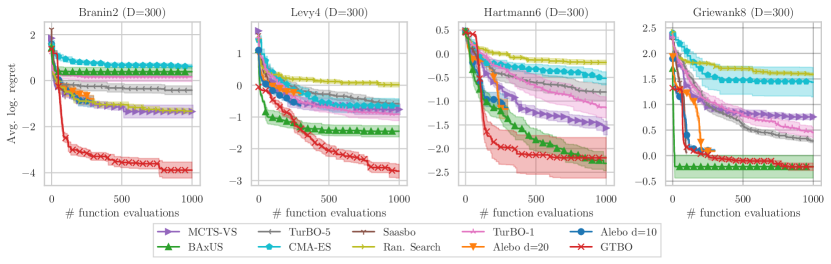
Figure 3: After finding the correct active dimensions, GTBO optimizes efficiently on synthetic noisy benchmarks (Branin2, Levy4, Hartmann6, and Griewank8). Mean and standard error of average log regret is plotted for each method over 100 iterations.

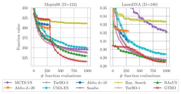
Figure 4: GTBO outperforms competitors in real-world experiments. Notably, the performance on Mopta08 increases by a large amount right after GT at iteration 300, suggesting that the dimensions found during the GT are highly relevant. As the default configuration on LassoDNA performs well, the performance increase after group testing is not as visually apparent.

We show that identifying the relevant variables can drastically improve optimization performance. Figure 4 shows the performance of GTBO and competitors on the real-world benchmarks, Figure 3 on the synthetic benchmarks. The results show the incumbent function value for each of the methods, averaged over ten repeated trials. We plot the true average incumbent function values on the noisy benchmarks without observation noise.

Note that Griewank has its optimum in the center of the search space. To not gain an unfair advantage, we run GTBO with a non-standard default away from the optimum. However, having the optimum in the center means that all possible projections will contain the optimum, which boosts the projection-based methods Alebo and BAxUS.

Figure 4 shows that GTBO performs well on real-world benchmarks. Note the drop directly after the group testing phase, indicating that knowing the correct active dimensions drastically speeds up optimization. In the real-world experiments, especially LassoDNA, the inactive variables still affect the function value. Appendix B shows that GTBO suffers a slight performance drop when using the stronger priors for the inactive dimensions. GTBO uses the center of the search space as a default point for the group testing phase, a decent point in LassoDNA. Note, however, that GTBO outperforms the competitors with a faster optimization performance even after starting from a worse solution after the group testing phase.

4.4 Sensitivity analysis

We explore the sensitivity of GTBO to the output noise and problem size by running it on the Levy4 synthetic benchmark extended to 100 dimensions, with a noise standard deviation of 0.1, and varying the properties of interest. In Figure 5, we show how the percentage of correctly predicted variables evolves with the number of tests $t$ for different functional properties. Correctly classified is defined here as having a probability of less than 1% if inactive or above 90% if active. GTBO shows to be robust with respect to lower noise levels but breaks down when the noise grows too large. As expected, higher function dimensionality and number of active dimensions increases the time until convergence. Note that the signal and noise variance estimates build on the assumption that there are a maximum of $\sqrt{D}$ active dimensions, which does not hold in the case with 32 active dimensions.

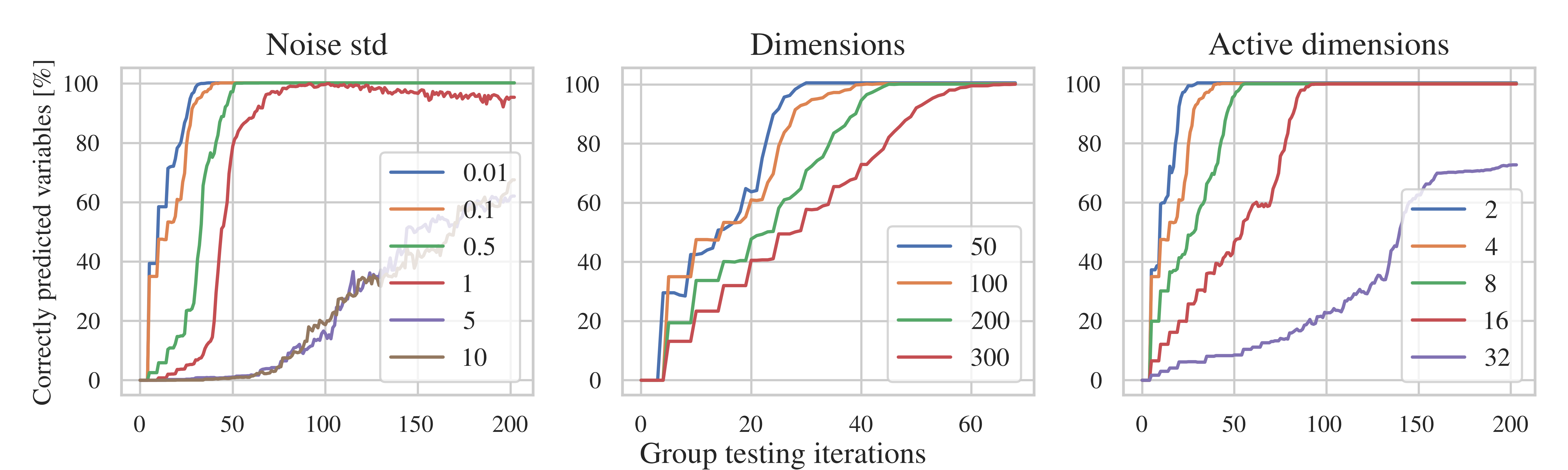
Figure 5: Sensitivity analysis for GTBO. The average percentage of correctly classified variables is displayed for an increasing number of group testing iterations. The percentage is ablated for (left) various levels of output noise, (middle) number of total dimensions, and (right) number of effective dimensions. Each legend shows the configurations of the respective parameter.

5 Discussion

Optimizing expensive-to-evaluate high-dimensional black-box functions is a challenge for applications in industry and academia. We propose GTBO, a novel BO method that explicitly exploits the structure of a sparse axis-aligned subspace to reduce the complexity of an application in high dimensions. GTBO is inspired by the field of group testing in which one aims to find infected individuals by conducting pooled tests but adapts it to the field of Bayesian optimization.

GTBO quickly detects active and inactive variables and shows robust optimization performance in synthetic and real-world settings. Furthermore, an important by-product is that users learn what dimensions of their applications are relevant and, consequently, learn something fundamental about their application. Since GTBO allows for user priors on the activeness of dimensions, we will explore the potential for increasing sample efficiency by including application-specific beliefs.

Appendix A The GTBO Algorithm

This section describes the group testing phase of the GTBO algorithm in additional detail.

0:  black-box function $f:\mathcal{X}\xrightarrow{}\mathbb{R}$, number of default configuration evaluations $n_{\text{def}}$, number of group tests $T$, number of particles $M$, prior distribution $p^{0}(\bm{\xi})$

0:  estimate of active dimensions $\bm{\gamma}$, posterior distribution $\hat{p}^{T}$

  for $j\in\{1\ldots n_{\text{def}}\}$ do

     $y_{\text{def}}^{(i)}=y(\bm{x}_{\text{def}})$

  end for

  $\hat{f}(\bm{x}_{\text{def}})\leftarrow\frac{1}{n_{\text{def}}}\sum_{i=1}^{n_{\text{def}}}y_{\text{def}}^{(i)}$

  

  split the dimensions into $3\lfloor\sqrt{D}\rfloor$ bins $B$

  for $j\in\{1\ldots|B|\}$ do

     $y_{\text{bin}}^{(j)}=y(\bm{x}_{\text{def}}\oplus\alpha b_{j})$ $\triangleright\,\,$ a random perturbation along the dimensions in bin $b_{j}$

  end for

  sort (asc.) $y_{\text{bin}}^{(j)}$

  $\hat{\sigma}_{n}^{2}\leftarrow\texttt{var}(y_{\text{bin}}^{(1)},\ldots,y_{\text{bin}}^{(2\lfloor\sqrt{D}\rfloor)})$

  $\hat{\sigma}^{2}\leftarrow\texttt{var}(y_{\text{bin}}^{(2\lfloor\sqrt{D}\rfloor+1)},\ldots,y_{\text{bin}}^{(3\lfloor\sqrt{D}\rfloor)})$

  

  $\bm{\xi}_{1},\ldots,\bm{\xi}_{M}\sim\hat{p}^{0}(\bm{\xi})$

  $\omega_{1},\ldots,\omega_{M}\leftarrow\frac{1}{M}$ $\triangleright\,\,$ initial particle weights

  for all $t\in\{1,\ldots,T\}$ do

     $\bm{g}^{*}\leftarrow$ maximize_mi$(\bm{\xi}_{1},\ldots,\bm{\xi}_{M})$ $\triangleright\,\,$ find a group that maximizes MI

     $\bm{x}_{t}\leftarrow$ create using Eq. (1) and $\bm{g}^{*}$

     $z_{t}\leftarrow f(\bm{x}_{t})+\varepsilon-\hat{f}(\bm{x}_{\text{def}})$

     $(\bm{\xi}_{i},\omega_{i})_{i\in[M]}\leftarrow\texttt{resample}(\bm{z}_{t},(\bm{\xi}_{i},\omega_{i})_{i\in[M]})$

     $\hat{p}^{t}\leftarrow$ marginal$((\bm{\xi}_{i},\omega_{i})_{i\in[M]})$ $\triangleright\,\,$ get marginals

  end for

  $\bm{\gamma}\leftarrow(\delta_{p^{T}(\bm{\xi}_{1})\geq\eta},\ldots,\delta_{p^{T}(\bm{\xi}_{D})\geq\eta})$ $\triangleright\,\,$ check which dimensions are active

Algorithm 1 Group testing phase

Appendix B Comparison with feature importance algorithms

We compare the performance of the group testing phase with the established feature importance analysis methods XGBoost [Chen and Guestrin, 2016] and fAnova [Hutter et al., 2014]. Since fAnova’s stability degrades with increasing dimensionality, we run these methods on the 100-dimensional version of the synthetic benchmarks: Branin2 (noise std 0.5), Griewank8 (noise std 0.5), Levy4 (noise std 0.1), and Hartmann6 (noise std 0.01).

Figure 6(a) shows the results of fAnova and XGBoost on the 100-dimensional version of Hartmann6 with added output noise. In accordance with our results, both methods flag the third dimension as not more important than the added input dimensions (dimensions 7-100 with no impact on the function value). Additionally, fAnova also seems to “switch off” the second dimension.

[width=]svg-inkscape/imp_HartmannEffectiveDim_svg-tex.pdf_tex

((a)) Hartmann6

[width=]svg-inkscape/imp_BraninEffectiveDim_svg-tex.pdf_tex

((b)) Branin2

[width=]svg-inkscape/imp_LevyEffectiveDim_svg-tex.pdf_tex

((c)) Levy4

[width=]svg-inkscape/imp1_GriewankEffectiveDim_svg-tex.pdf_tex

((d)) Griewank8

Figure 6: XGBoost and fAnova feature importance analysis on the 100-dimensional version of different synthetic benchmarks, averaged over 20 repetitions. Only the first 20 dimensions are shown.

On Branin2 (Fig. 6(b)), both methods detect the correct dimensions (the first and second dimensions). Furthermore, all other dimensions have zero importance, and the methods find the correct partitioning earlier than for Hartmann6. Similarly to Hartmann6, both methods fail to detect an active dimension (the fourth dimension).

On Griewank8, fAnova does not terminate gracefully. Therefore, we only discuss XGBoost for Griewank8. After 300 iterations, XGBoost only detects six dimensions reliably as active. The other two dimensions are determined to be not more important than the added dimensions. The marginals found by GTBO are shown in Fig. 7. Compared conventional feature importance analysis methods, GTBO detects all active dimensions with high probability.

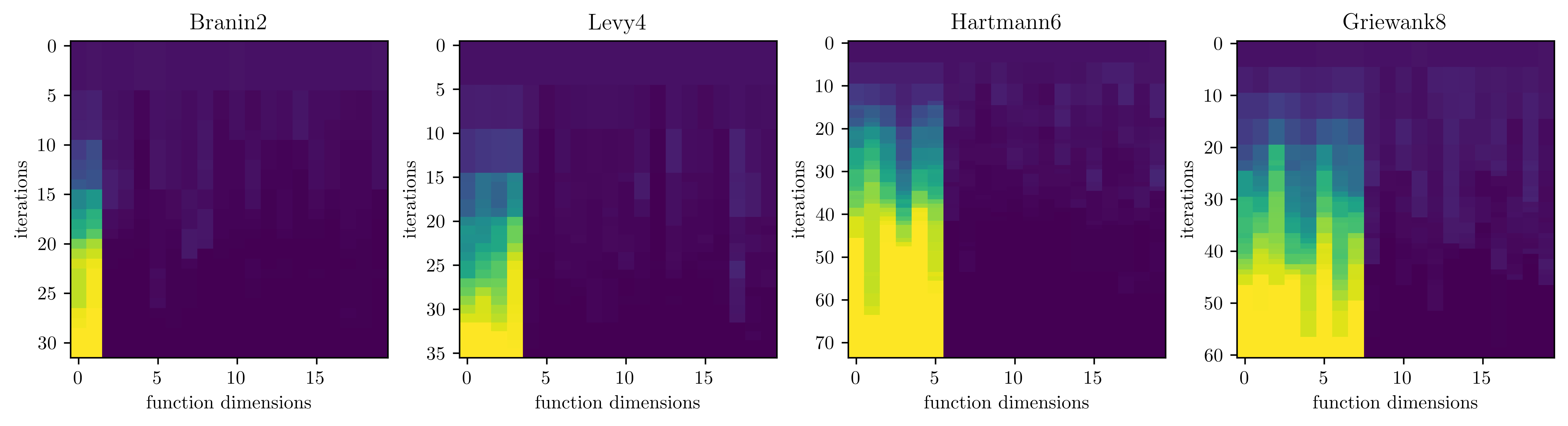
Figure 7: GTBO-marginals of the first 20 dimensions., averaged over 10 repetitions. If the group testing phase ends early, the last marginals are repeated to match the length of the longest group testing phase.

Appendix C Number of active variables

Here, we show the average number of active dimensions throughout the group testing phase. Given that the acceptance threshold of 0.5 is much higher than the initial probability of acceptance of 0.05, dimensions once considered active are rarely later considered inactive again, resulting in a close to monotonically increasing number of active dimensions.

[width=]svg-inkscape/nactive_svg-tex.pdf_tex

Figure 8: Evolution average number of active variables during the group testing phase (10 repetitions). The synthetic benchmarks find the correct number of active variables, whereas the real-world benchmarks find a significantly higher number.

Appendix D Complementary Prior Experiments

In addition to the lengthscale priors used in Section 4.3, we run the real-world experiments with the complementary priors, i.e., $\mathcal{LN}(7,1)$ length scale priors for the real-world and $\mathcal{LN}(3,1)$ length scale priors for the synthetic experiments.

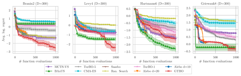
Figure 9: Endowed with a weaker $\mathcal{LN}(3,1)$ length scale prior, GTBO shows convincing yet slower optimization performance on the noisy synthetic benchmarks (Branin2, Levy4, Hartmann6, and Griewank8).

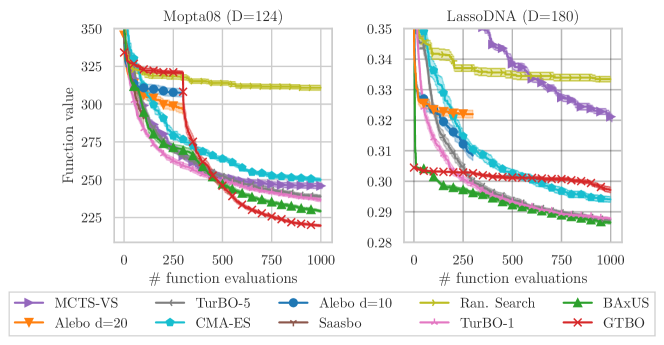
Figure 10: A stronger $\mathcal{LN}(7,1)$ length scale prior still allows GTBO to achieve state-of-the-art performance on Mopta08 and robust performance on LassoDNA.

Figure 9 shows GTBO’s performance on the synthetic benchmarks when equipped with a weaker $\mathcal{LN}(3,1)$ length scale prior. The weaker prior “switches on” dimensions that are found to be inactive during the group-testing phase and slows down optimization performance. Contrary to this, the stronger $\mathcal{LN}(7,1)$ prior for the off-dimensions for real-world benchmarks (Figure 10) inhibits GTBO in its ability to optimize “off-dimensions”. We suspect that LassoDNA benefits more from optimizing those dimensions that Mopta08, hence the stronger performance degradation on LassoDNA.

Appendix E Run times

In this section, we show the average run of GTBO. Note that the SMC resampling is a part of the group testing phase, and as such, the total algorithm time is the GT time plus the BO time. We do batch evaluations in the GT phase as described in Section 3, with a maximum of five groups tested before resampling. This significantly reduces the SMC resample time.

Benchmark	GT time [h]	SMC resample time [h]	BO time [h]
Branin2 (300D)	1.94	0.583	9.31
Levy4 (300D)	2.33	0.603	10.8
Hartmann6 (300D)	3.29	1.14	14.1
Griewank8 (300D)	2.41	0.846	9.08
Mopta08 (124D)	5.70	4.74	7.95
LassoDNA (180D)	8.92	7.06	10.2

Table 1: Average GTBO runtimes. Group testing time is on the same order of magnitude as the time allocated towards BO. For BO, the $\mathcal{O}(D^{2})$ complexity of Quasi-Newton-based acquisition function optimization dominates the runtime.

References

- Aldridge et al. (2019) M. Aldridge, O. Johnson, J. Scarlett, et al. Group testing: an information theory perspective. Foundations and Trends® in Communications and Information Theory, 15(3-4):196–392, 2019.
- Bakshy et al. (2018) E. Bakshy, L. Dworkin, B. Karrer, K. Kashin, B. Letham, A. Murthy, and S. Singh. AE: A domain-agnostic platform for adaptive experimentation. In Conference on Neural Information Processing Systems, pages 1–8, 2018.
- Balandat et al. (2020) M. Balandat, B. Karrer, D. Jiang, S. Daulton, B. Letham, A. G. Wilson, and E. Bakshy. BoTorch: A framework for efficient Monte-Carlo Bayesian optimization. Advances in neural information processing systems, 33:21524–21538, 2020.
- Balding et al. (1996) D. Balding, W. Bruno, D. Torney, and E. Knill. A comparative survey of non-adaptive pooling designs. In Genetic mapping and DNA sequencing, pages 133–154. Springer, 1996.
- Bansal et al. (2022) A. Bansal, D. Stoll, M. Janowski, A. Zela, and F. Hutter. JAHS-Bench-201: A Foundation For Research On Joint Architecture And Hyperparameter Search. In Thirty-sixth Conference on Neural Information Processing Systems Datasets and Benchmarks Track, 2022.
- Berkenkamp et al. (2021) F. Berkenkamp, A. Krause, and A. Schoellig. Bayesian Optimization with Safety Constraints: Safe and Automatic Parameter Tuning in Robotics. Machine Learning, 06 2021. doi: 10.1007/s10994-021-06019-1.
- Binois and Wycoff (2022) M. Binois and N. Wycoff. A survey on high-dimensional gaussian process modeling with application to bayesian optimization. ACM Transactions on Evolutionary Learning and Optimization, 2(2):1–26, 2022.
- Bouhlel et al. (2016) M. A. Bouhlel, N. Bartoli, A. Otsmane, and J. Morlier. Improving kriging surrogates of high-dimensional design models by partial least squares dimension reduction. Structural and Multidisciplinary Optimization, 53:935–952, 2016.
- Burger et al. (2020) B. Burger, P. M. Maffettone, V. V. Gusev, C. M. Aitchison, Y. Bai, X. Wang, X. Li, B. M. Alston, B. Li, R. Clowes, et al. A mobile robotic chemist. Nature, 583(7815):237–241, 2020.
- Calandra et al. (2014) R. Calandra, N. Gopalan, A. Seyfarth, J. Peters, and M. Deisenroth. Bayesian gait optimization for bipedal locomotion. In P. Pardalos and M. Resende, editors, Proceedings of the Eighth International Conference on Learning and Intelligent Optimization (LION’14), 2014.
- Chen and Guestrin (2016) T. Chen and C. Guestrin. Xgboost: A scalable tree boosting system. In Proceedings of the 22nd acm sigkdd international conference on knowledge discovery and data mining, pages 785–794, 2016.
- Chen et al. (2018) Y. Chen, A. Huang, Z. Wang, I. Antonoglou, J. Schrittwieser, D. Silver, and N. de Freitas. Bayesian Optimization in AlphaGo. CoRR, abs/1812.06855, 2018.
- Clifford et al. (2010) R. Clifford, K. Efremenko, E. Porat, and A. Rothschild. Pattern matching with don’t cares and few errors. Journal of Computer and System Sciences, 76(2):115–124, 2010.
- Constantine et al. (2015) P. G. Constantine, A. Eftekhari, and M. B. Wakin. Computing active subspaces efficiently with gradient sketching. In 2015 IEEE 6th International Workshop on Computational Advances in Multi-Sensor Adaptive Processing (CAMSAP), pages 353–356. IEEE, 2015.
- Cuturi et al. (2020) M. Cuturi, O. Teboul, and J.-P. Vert. Noisy Adaptive Group Testing using Bayesian Sequential Experimental Design. CoRR, abs/2004.12508, 2020.
- Del Moral et al. (2006) P. Del Moral, A. Doucet, and A. Jasra. Sequential monte carlo samplers. Journal of the Royal Statistical Society: Series B (Statistical Methodology), 68(3):411–436, 2006.
- Djolonga et al. (2013) J. Djolonga, A. Krause, and V. Cevher. High-dimensional gaussian process bandits. Advances in neural information processing systems, 26, 2013.
- Dorfman (1943) R. Dorfman. The detection of defective members of large populations. The Annals of mathematical statistics, 14(4):436–440, 1943.
- Ejjeh et al. (2022) A. Ejjeh, L. Medvinsky, A. Councilman, H. Nehra, S. Sharma, V. Adve, L. Nardi, E. Nurvitadhi, and R. A. Rutenbar. HPVM2FPGA: Enabling True Hardware-Agnostic FPGA Programming. In Proceedings of the 33rd IEEE International Conference on Application-specific Systems, Architectures, and Processors, 2022.
- Eriksson and Jankowiak (2021) D. Eriksson and M. Jankowiak. High-dimensional Bayesian optimization with sparse axis-aligned subspaces. In Uncertainty in Artificial Intelligence, pages 493–503. PMLR, 2021.
- Eriksson et al. (2019) D. Eriksson, M. Pearce, J. Gardner, R. D. Turner, and M. Poloczek. Scalable global optimization via local bayesian optimization. Advances in neural information processing systems, 32, 2019.
- Frazier (2018) P. I. Frazier. A tutorial on Bayesian optimization. arXiv preprint arXiv:1807.02811, 2018.
- Hansen and Ostermeier (1996) N. Hansen and A. Ostermeier. Adapting arbitrary normal mutation distributions in evolution strategies: The covariance matrix adaptation. In Proceedings of IEEE international conference on evolutionary computation, pages 312–317. IEEE, 1996.
- Hansen et al. (2022) N. Hansen, yoshihikoueno, ARF1, K. Nozawa, L. Rolshoven, M. Chan, Y. Akimoto, brieglhostis, and D. Brockhoff. CMA-ES/pycma: r3.2.2, Mar. 2022.
- Huber et al. (2008) M. F. Huber, T. Bailey, H. Durrant-Whyte, and U. D. Hanebeck. On entropy approximation for Gaussian mixture random vectors. In 2008 IEEE International Conference on Multisensor Fusion and Integration for Intelligent Systems, pages 181–188. IEEE, 2008.
- Hutter et al. (2014) F. Hutter, H. Hoos, and K. Leyton-Brown. An efficient approach for assessing hyperparameter importance. In International conference on machine learning, pages 754–762. PMLR, 2014.
- Hvarfner et al. (2022) C. Hvarfner, F. Hutter, and L. Nardi. Joint entropy eearch for maximally-informed bayesian optimization. In Proceedings of the 36th International Conference on Neural Information Processing Systems, 2022.
- Hvarfner et al. (2023) C. Hvarfner, E. Hellsten, F. Hutter, and L. Nardi. Self-correcting bayesian optimization through bayesian active learning. In Thirty-seventh Conference on Neural Information Processing Systems, 2023. URL https://openreview.net/forum?id=dX9MjUtP1A.
- Jones (2008) D. R. Jones. Large-scale multi-disciplinary mass optimization in the auto industry. In MOPTA 2008 Conference (20 August 2008), 2008.
- Kandasamy et al. (2018) K. Kandasamy, W. Neiswanger, J. Schneider, B. Poczos, and E. P. Xing. Neural architecture search with bayesian optimisation and optimal transport. Advances in neural information processing systems, 31, 2018.
- Letham et al. (2018) B. Letham, K. Brian, G. Ottoni, and E. Bakshy. Constrained Bayesian optimization with noisy experiments. Bayesian Analysis, 2018.
- Letham et al. (2020) B. Letham, R. Calandra, A. Rai, and E. Bakshy. Re-examining linear embeddings for high-dimensional Bayesian optimization. Advances in neural information processing systems, 33:1546–1558, 2020.
- Liu (1996) J. S. Liu. Peskun’s theorem and a modified discrete-state Gibbs sampler. Biometrika, 83(3), 1996.
- Macula and Popyack (2004) A. J. Macula and L. J. Popyack. A group testing method for finding patterns in data. Discrete applied mathematics, 144(1-2):149–157, 2004.
- Mayr et al. (2022) M. Mayr, C. Hvarfner, K. Chatzilygeroudis, L. Nardi, and V. Krueger. Learning skill-based industrial robot tasks with user priors. IEEE 18th International Conference on Automation Science and Engineering, 2022. URL https://arxiv.org/abs/2208.01605.
- Nardi et al. (2019) L. Nardi, D. Koeplinger, and K. Olukotun. Practical design space exploration. In 2019 IEEE 27th International Symposium on Modeling, Analysis, and Simulation of Computer and Telecommunication Systems (MASCOTS), pages 347–358. IEEE, 2019.
- Nayebi et al. (2019) A. Nayebi, A. Munteanu, and M. Poloczek. A framework for Bayesian optimization in embedded subspaces. In International Conference on Machine Learning, pages 4752–4761. PMLR, 2019.
- Negoescu et al. (2011) D. M. Negoescu, P. I. Frazier, and W. B. Powell. The knowledge-gradient algorithm for sequencing experiments in drug discovery. INFORMS Journal on Computing, 23(3):346–363, 2011.
- Ngo and Du (2000) H. Q. Ngo and D.-Z. Du. A survey on combinatorial group testing algorithms with applications to DNA library screening. Discrete mathematical problems with medical applications, 55:171–182, 2000.
- Papenmeier et al. (2022) L. Papenmeier, L. Nardi, and M. Poloczek. Increasing the Scope as You Learn: Adaptive Bayesian Optimization in Nested Subspaces. In Advances in Neural Information Processing Systems, 2022.
- Papenmeier et al. (2023) L. Papenmeier, L. Nardi, and M. Poloczek. Bounce: a Reliable Bayesian Optimization Algorithm for Combinatorial and Mixed Spaces. arXiv preprint arXiv:2307.00618, 2023.
- Pedrielli and Ng (2016) G. Pedrielli and S. H. Ng. G-STAR: A new kriging-based trust region method for global optimization. In 2016 Winter Simulation Conference (WSC), pages 803–814. IEEE, 2016.
- Regis (2016) R. G. Regis. Trust regions in Kriging-based optimization with expected improvement. Engineering optimization, 48(6):1037–1059, 2016.
- Ru et al. (2020) B. Ru, X. Wan, X. Dong, and M. Osborne. Interpretable neural architecture search via bayesian optimisation with weisfeiler-lehman kernels. arXiv preprint arXiv:2006.07556, 2020.
- Russell (2010) S. J. Russell. Artificial intelligence a modern approach. Pearson Education, Inc., 2010.
- Scarlett (2018) J. Scarlett. Noisy adaptive group testing: Bounds and algorithms. IEEE Transactions on Information Theory, 65(6):3646–3661, 2018.
- Šehić et al. (2022) K. Šehić, A. Gramfort, J. Salmon, and L. Nardi. LassoBench: A High-Dimensional Hyperparameter Optimization Benchmark Suite for Lasso. In First Conference on Automated Machine Learning (Main Track), 2022.
- Shahriari et al. (2016) B. Shahriari, A. Bouchard-Cote, and N. de Freitas. Unbounded Bayesian optimization via regularization. In A. Gretton and C. Robert, editors, Proceedings of the Seventeenth International Conference on Artificial Intelligence and Statistics (AISTATS), volume 51, pages 1168–1176. Proceedings of Machine Learning Research, 2016.
- Song et al. (2022) L. Song, K. Xue, X. Huang, and C. Qian. Monte Carlo Tree Search based Variable Selection for High Dimensional Bayesian Optimization. arXiv preprint arXiv:2210.01628, 2022.
- Ulmasov et al. (2016) D. Ulmasov, C. Baroukh, B. Chachuat, M. P. Deisenroth, and R. Misener. Bayesian optimization with dimension scheduling: Application to biological systems. In Computer Aided Chemical Engineering, volume 38, pages 1051–1056. Elsevier, 2016.
- Wang et al. (2016) Z. Wang, F. Hutter, M. Zoghi, D. Matheson, and N. De Feitas. Bayesian optimization in a billion dimensions via random embeddings. Journal of Artificial Intelligence Research, 55:361–387, 2016.
- Wolf (1985) J. Wolf. Born again group testing: Multiaccess communications. IEEE Transactions on Information Theory, 31(2):185–191, 1985.
- Wycoff et al. (2021) N. Wycoff, M. Binois, and S. M. Wild. Sequential learning of active subspaces. Journal of Computational and Graphical Statistics, 30(4):1224–1237, 2021.
- Zhang et al. (2020) Y. Zhang, D. W. Apley, and W. Chen. Bayesian optimization for materials design with mixed quantitative and qualitative variables. Scientific reports, 10(1):1–13, 2020.
- Zhou et al. (2014) Y. Zhou, U. Porwal, C. Zhang, H. Q. Ngo, X. Nguyen, C. Ré, and V. Govindaraju. Parallel feature selection inspired by group testing. Advances in neural information processing systems, 27, 2014.