Exploring the Hubble Tension: A Novel Approach through Cosmological Observations

Abstract

The simplest cosmological model ($\Lambda$CDM) is well-known to suffer from the Hubble tension, namely an almost $5\sigma$ discrepancy between the (model-based) early-time determination of the Hubble constant $H_{0}$ and its late-time (and model-independent) determination. To circumvent this, we introduce an additional energy source that varies with the redshift as $(1+z)^{n}$, where $0<n<3$, and test it against the Pantheon Compilation of Type Ia Supernovae as well as the CMBR observations (at $z\approx 1100$). The deduced $H_{0}$ is now well-consistent with the value obtained from local observations of Cepheid variables. Suggesting a non-zero value for the curvature density parameter, positive (negative) for $n>2$ ($n<2$), the resolution is also consistent with the BAO data.

I Introduction

The Hubble constant $H_{0}$ has been used for almost $90$ years to describe the current rate of expansion of the Universe Lemaitre (1927); Hubble (1929). However, while the precise measurement of the Cosmic Microwave Background Radiation (CMBR) supplemented by the standard ($\Lambda$CDM) cosmological model suggests that $H_{0}=67.66\pm 0.42$ $\mathrm{km}\ \mathrm{s}^{-1}\mathrm{Mpc}^{-1}$ (Hinshaw et al., 2013; Aghanim et al., 2020), a model-independent determination using distance ladders alongwith Type Ia supernovae (SNe) data and the SH0ES project yields $H_{0}=73.04\pm 1.04$ $\mathrm{km}\ \mathrm{s}^{-1}\mathrm{Mpc}^{-1}$ Scolnic et al. (2018); Riess et al. (2022). This discrepancy (nearly $5\sigma$) between the outcomes of two profoundly different measurements (early time vs. local) is termed as the Hubble tension.

Unless the discrepancy is just an artefact of unresolved systematics, an explanation would call for some unknown physics effects Vagnozzi (2020). However, given the internal accuracy of the data, maintaining the consistency of the redshift ($z$) dependent observable $H(z)$ at both ends of the distance scale imposes severe constraints on the nature of the new physics models. This has led to the use of further model-independent methods for determining $H_{0}$, an example being the age of the earliest stellar populations in our galaxy Trenti et al. (2015); Jimenez et al. (2019); Valcin et al. (2020); Bernal et al. (2021); Boylan-Kolchin and Weisz (2021). However, the majority of the age measurements rely on objects at higher redshifts, which can constrain other cosmological parameters*1995Natur.376..399B; *1995GReGr..27.1137K; *1996Natur.381..581D; *1999ApJ...521L..87A; *2000MNRAS.317..893L; *2002ApJ...573...37J; *2003ApJ...593..622J; *2004PhRvD..70l3501C; *2005MNRAS.362.1295F; *2006PhLB..633..436J; *2014A&A...561A..44B; *2015AJ....150...35W; *2017JCAP...03..028R; *2020MNRAS.496..888N; *2021ApJ...908...84V, but none serve to resolve the Hubble tension Di Valentino et al. (2021); Kamionkowski and Riess (2022); Hu and Wang (2023).

There are two primary methods for constructing a consistent model of the universe that would account for both the dynamics of the local observations, namely the current accelerated expansion of the universe as well as early universe observations. Einstein’s minimal gravitational action can be modified, and extended gravity theories constructed Nojiri and Odintsov (2007); De Felice and Tsujikawa (2010); Capozziello and De Laurentis (2011); Cai et al. (2016). The alternative is to replace the cosmological constant by a matter component exerting negative pressure and known as dark energy (DE) Carroll (2001); Peebles and Ratra (2003); Copeland et al. (2006); Li et al. (2013). Despite numerous efforts, there is still no preferred dark energy model that can precisely describe the universe’s dynamical processes, including the Hubble tension.

Four primary components define the $\Lambda$CDM model: radiation, dust, scalar curvature, and the cosmological constant. Each component is barotropic, i.e. the pressure is proportional to energy density: $P=w\rho c^{2}$, where $w$ is known as the equation of state parameter for the fluid. For radiation, $w_{r}=1/3,$ whereas $w_{m}=0,w_{k}=-1/3$ and $w_{\Lambda}=-1,$ respectively, are the values for dust matter, scalar curvature, and the cosmological constant. While fits of the $\Lambda$CDM ansatz with the early (Hinshaw et al., 2013; Aghanim et al., 2020) as well as late-time observations Scolnic et al. (2018); Riess et al. (2022) are consistent with a vanishing curvature contribution, we do not, a priori demand this. Furthermore, to alleviate the tension, we admit the existence, in the system, of a non-negligible amount of another barotropic fluid with the equation of state parameter $w_{n}$. The Universe was already dominated by the dust matter ($w_{m}=0$) during the recombination era, whereas the current Universe is assumed to be driven by the cosmological constant $(w_{\Lambda}=-1)$. Since the tension arises from the overlap of these two eras, it stands to reason that any component capable of effecting a significant change in the dynamics should lie between dust and cosmological constant in its behavior. In other words, $-1<w_{n}<0$ is preferred. As the energy density of the barotropic fluid $\rho\propto a^{-3(1+w)},$ where $a(t)$ is the scale factor, it follows that the energy density of the newly assumed fluid satisfies $\rho_{n}\propto(1+z)^{n},$ where $0<n<3$.

This paper is organized as follows: in section II, we describe the dataset (Pantheon) and methodology (Markov Chain Monte Carlo) used in this work. The obtained results, we present in Sec. III. Finally, Sec. IV discusses the main conclusions and summarizes.

II Dataset and Methodology

II.1 Type Ia Supernovae Dataset

Type Ia supernovae (SNe) being standard candles, the luminosity distance measurements for these have been crucial in establishing the current cosmic acceleration. The observable of interest is the distance modulus $\mu_{\rm SNe}$ defined as the difference between the apparent and absolute magnitude of the individual supernova. This can be related to the observed rest frame $B$-band peak magnitude $m_{B}(z)$, the time stretching of the light curve ($X_{1})$ and the SNe color at maximum brightness ($C$) through Scolnic et al. (2018)

$$\mu_{\rm SNe}(z)=m_{B}(z)+\alpha\cdot X_{1}-\beta\cdot C-M_{B}$$ (1)

The absolute $B$-band magnitude or the luminosity is almost independent of the redshift Tutusaus et al. (2019); Kumar et al. (2022), and is normally distributed with a very small spread, viz., $M_{B}=-19.220\pm 0.042$ Benevento et al. (2020). The nuisance parameters $\alpha$ and $\beta$ associated with the variables $X_{1}$ and $C$ have been marginalized for the Pantheon dataset Scolnic et al. (2018) comprising 1048 Type Ia SNe in the redshift range $0.01\leq z\leq 2.26$, and eventually calibrated to be zero. Thus, the expression for the observed distance modulus essentially reduces to just $\mu_{\rm SNe}(z)=m_{B}(z)-M_{B}$.

It is convenient to define a distance modulus variable $d_{L}(z)$ through

$$d_{L}^{\mathrm{obs}}\left(z\right)=10^{\left(\mu_{\rm SNe}-25\right)/5}~{}~{}(\text{Mpc})\ ,$$ (2)

with the attendant uncertainty being determined by $\sigma_{m_{B}}$ alone. The observations constituting the Pantheon database are depicted in Fig. 1.

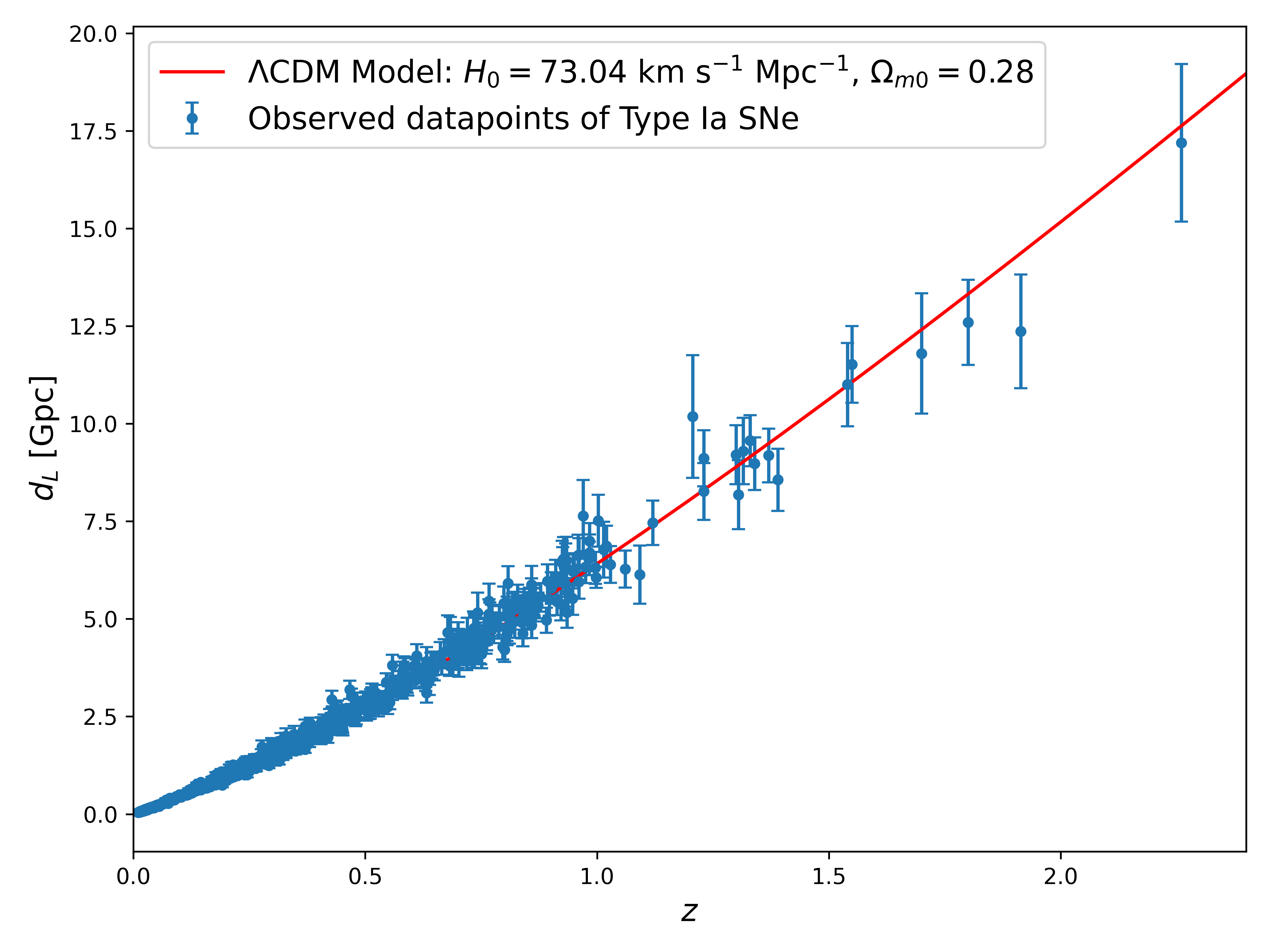
Figure 1: The luminosity distance measurements of Type Ia SNe in the redshift range $0.01\leq z\leq 2.26$. The solid red line is the theoretical curve for the flat $\Lambda$CDM model with $H_{0}=73.04$ $\mathrm{km}\ \mathrm{s}^{-1}\mathrm{Mpc}^{-1}$ and $\Omega_{m0}=0.28$.

II.2 Parameter Estimation

With the Friedmann equation giving a simple relation between $H(z)$ and the energy density (including that due to a cosmological constant), it is customary to posit simple equations of state (barotropic fluids) for the matter components leading to straightforward expressions for the respective energy densities in terms of $z$. In the present instant, we invoke an additional contribution, namely $\Omega_{n}(z)=\Omega_{n0}(1+z)^{n}$, where $\Omega_{n0}$ denotes its value at the current epoch, i.e., at $z=0$. We have, then,

$$H^{2}(z) = H^{2}_{0}\left[\Omega_{r0}(1+z)^{4}+\Omega_{m0}(1+z)^{3}+\Omega_{\Lambda}\right.$$ (3)

$$\left.\hskip 20.0pt+\Omega_{k0}(1+z)^{2}+\Omega_{n0}(1+z)^{n}\right],$$

where, as usual, $\Omega_{r0},~{}\Omega_{m0},$ and $\Omega_{k0}$ are the current energy density parameters due to radiation, matter, and curvature respectively. And while $\Omega_{k0}\approx 0$ within the $\Lambda$CDM, a priori it is not clear that it would continue to be so in the revised context. Furthermore, $\Omega_{r0}+\Omega_{m0}+\Omega_{k0}+\Omega_{\Lambda}+\Omega_{n0}=1$, allowing us to eliminate one variable in terms of the others, and this we choose to be $\Omega_{n0}$. The extant data is insensitive to the exact value of $\Omega_{r0}$ (since $\Omega_{r}$ is already negligibly small by the recombination epoch and plays little or no role in parameter estimation), and, hence, for the subsequent numerical analyses, we use just the central value viz. $\Omega_{r0}=8.5\times 10^{-5}$.

Given the expression above for $H(z)$, one can define the luminosity distance theoretically as

$$d_{L}^{\text{th}}(z;\mathcal{P})=\dfrac{c(1+z)}{H_{0}\sqrt{\Omega_{k0}}}\,\sinh\left[H_{0}\sqrt{\Omega_{k0}}\int_{0}^{z}\dfrac{dz^{\prime}}{H(z^{\prime})}\right],$$ (4)

where $\mathcal{P}\equiv\{H_{0},~{}\Omega_{m0},~{}\Omega_{k0},~{}\Omega_{\Lambda}\}$, $c$ is the speed of light.

We may now determine the parameters of the model by minimizing

$$\chi^{2}\left(\mathcal{P}\right)=\sum_{i=1}^{N}\left(\dfrac{d_{L}^{\rm th}\left(z_{i};\mathcal{P}\right)-d_{L}^{\text{obs}}\left(z_{i}\right)}{\sigma_{{d_{L}}}^{\text{obs}}\left(z_{i}\right)}\right)^{2},$$ (5)

where the sum extends not only over the entire Pantheon database of Type Ia SNe, but also over distance measurements at the recombination era.

III Results

Our aim is to fit Eq. (3) for $H(z)$ to the data in the presence of a nonzero $\Omega_{n0}$ and to investigate whether a qualitative difference exists as compared to the standard $\Lambda$CDM (i.e., the limit of $\Omega_{n0}=0$). While it might be tempting to consider $n$ itself also as a continuous variable, we desist from doing so under the assumption that its value is decided by the underlying theory, whose structure we remain agnostic about. Instead, we investigate the consequences for a few discrete values of $n$. We thus have four free parameters, namely $H_{0}$, $\Omega_{m0}$, $\Omega_{k0}$ and $\Omega_{\Lambda}$, with $\Omega_{n0}$ determined from the rest.

Param.	Best value [68% C.L.]
	$n=0.5$	$n=1.0$	$n=1.5$	$n=2.5$
$x$	$19427^{+471}_{-502}$	$19357^{+503}_{-482}$	$19291^{+501}_{-492}$	$19168^{+465}_{-456}$
$y$	$1399.7^{+29.6}_{-29.0}$	$1403.8^{+30.2}_{-30.2}$	$1408.0^{+31.8}_{-31.2}$	$1416.9^{+30.8}_{-30.4}$
$H_{0}$	$72.198^{+0.197}_{-0.191}$	$72.200^{+0.189}_{-0.187}$	$72.191^{+0.187}_{-0.186}$	$72.189^{+0.170}_{-0.173}$
$\Omega_{m0}$	$0.268^{+0.006}_{-0.006}$	$0.269^{+0.006}_{-0.006}$	$0.270^{+0.006}_{-0.006}$	$0.272^{+0.006}_{-0.006}$
$\Omega_{k0}$	$-0.024^{+0.061}_{-0.059}$	$-0.053^{+0.080}_{-0.079}$	$-0.126^{+0.129}_{-0.129}$	$0.132^{+0.064}_{-0.066}$
$\Omega_{\Lambda}$	$0.491^{+0.247}_{-0.261}$	$0.594^{+0.114}_{-0.117}$	$0.634^{+0.065}_{-0.065}$	$0.673^{+0.027}_{-0.026}$
$\Omega_{n0}$	$0.259^{+0.302}_{-0.312}$	$0.189^{+0.187}_{-0.189}$	$0.221^{+0.184}_{-0.187}$	$-0.077^{+0.048}_{-0.046}$
$\chi^{2}_{\nu}$	$0.9842$	$0.9846$	$0.9849$	$0.9859$

Table 1: The best fit values of $x$, $y$, $H_{0}$, $\Omega_{m0}$, $\Omega_{k0}$, $\Omega_{\Lambda 0}$ (along with the $68\%$ C.L. intervals) for different values of the parameter $n$. Also displayed are the deduced value of $\Omega_{n0}$ and the reduced $\chi^{2}$.

To this end, we employ the emcee-a Python implementation of a Markov Chain Monte Carlo Foreman-Mackey et al. (2013) using the Pantheon dataset Scolnic et al. (2018), augmented by the CMBR data (at $z\approx 1100$). At such large redshifts, $H(z)$ is determined primarily by the combination $y\equiv H_{0}^{2}\Omega_{m0}$, and the accuracy of the data leads to $y=1424.18\pm 31.37$. Hence, instead of $H_{0}$ and $\Omega_{m0}$, we use the combinations $x\equiv H_{0}^{2}/\Omega_{m0}$ and $y$. For $y$, we naturally use a Gaussian prior (with obvious parameters). For the rest, we use flat priors, albeit restricted to a certain interval, viz.

$$x\in[8000,22000]\ ,\quad\Omega_{k0}\in[-1,1]\ ,\quad\Omega_{\Lambda}\in[0,1]\ .$$ (6)

The flatness of the priors only reflect our ignorance of the said parameters. While it is tempting to use a Gaussian prior for $x$ as well, doing so would be tantamount to unduly favoring the $\Lambda$CDM model as the individual determination of $\{H_{0},\Omega_{m0}\}$ from the CMBR data that such a course would imply is implicitly dependent on the said model.

Before we discuss the individual cases, we summarise, in Table 1, part of the results of our MCMC analysis. This immediately allows us to infer several results:

• For all $n$, the obtained best fit value of $H_{0}$ (see Table 1) is consistent, within $1\sigma$, with that determined by the SH0ES survey. That these values are virtually independent of $n$, signals a robustness of the fit. This constitutes a central result of our analysis.

• That the fitted values of $\Omega_{m0}$ (again, virtually independent of $n$) are somewhat lower than that in the $\Lambda$CDM was to be expected and is but a consequence of the presence of the exotic matter.

• With the data from the CMBR observations playing an important role in the fitting and with the combination $y=H_{0}^{2}\Omega_{m0}$ largely determining the rate of expansion at that epoch, it was expected that the fitted value of $y$ would be close to that in $\Lambda$CDM and have only a tiny dependence on $n$ (see Table 1). This, in turn, also indicates why the increase in $H_{0}$ (vis-à-vis $\Lambda$CDM) needs to be accompanied by a decrease in $\Omega_{m0}$.

• The dependence on $n$ is, however, very pronounced for the best fit values of both $\Omega_{\Lambda}$ and $\Omega_{k0}$ (and, thereby, $\Omega_{n0}$). In particular, $\Omega_{\Lambda}$ deviates strongly from the $\Lambda$CDM value of $0.685$ as $n$ deviates from 3. This is understandable, for $n\to 3$ signals ordinary pressureless matter (dust), a situation indistinguishable from the $\Lambda$CDM. As $3-n$ increases, the new component becomes more and more exotic and contributes to suppress $\Omega_{\Lambda}$.

• Moving to a discussion for specific values of $n$, we start with $n=0.5$. The best fit point for $\Omega_{k0}$ points only marginally towards an open universe, with a flat universe being as probable. Similarly, the error bars on both $\Omega_{\Lambda}$ and $\Omega_{n0}$ are relatively large. This is not unexpected as $n=0.5$ inidicates an exotic matter that is almost cosmological constant-like. Consequently, the split between the two components is not very clearly demarcated. And while it is tempting to conclude that both $\Omega_{n0}$ and $\Omega_{k0}$ are consistent with vanishing values, note that the parameters are correlated and such a conclusion is not well supported (consider, for example, the departure of $\Omega_{m0}+\Omega_{\Lambda}$ from unity).

  

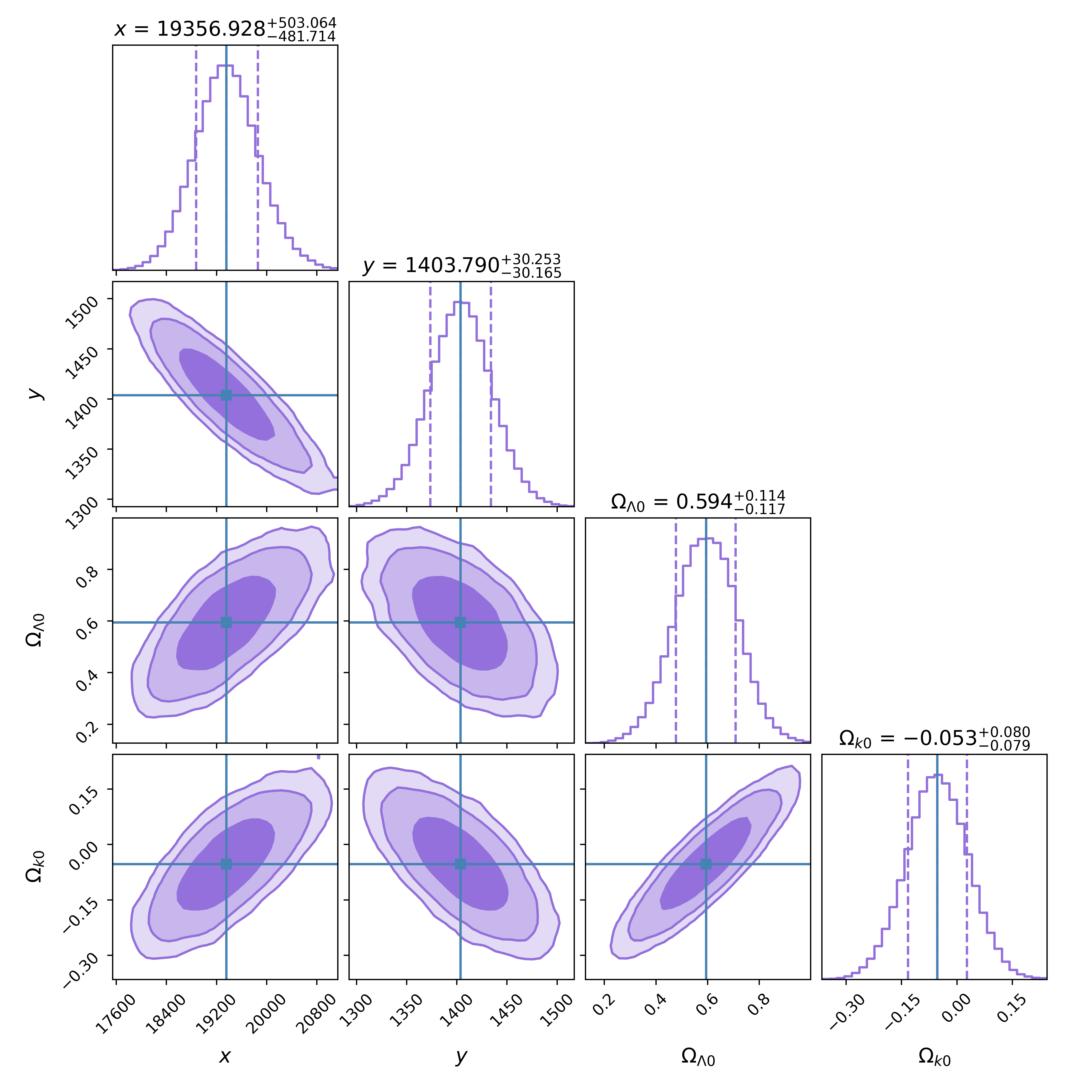
  Figure 2: The 1D and 2D posterior distributions of $x$, $y$, $\Omega_{k0}$, and $\Omega_{\Lambda 0}$ for $n=1$.

• For $n=1$, the posterior distributions for the parameters are shown in Fig. 2. The preferred value for $\Omega_{k0}$ has grown more negative (open universe), although a flat universe is still consistent within $0.7\sigma$. The substantial shift in $\Omega_{\Lambda}$ (as compared to the $n=0.5$ case) is accompanied by a compensatory shift in $\Omega_{n0}$ (and, to a smaller extent, that in $\Omega_{k0}$). These features are not surprising as an $n=1$ component could be imagined to be midway between a cosmological constant and a curvature contribution. Consequently, shifts in the latter would compensate for any deleterious effects due to $\Omega_{n0}$. Finally, as Fig. 2 shows, the parameters are indeed highly correlated.

• For $n=1.5$, the posteriors remain qualitatively similar, but are sharper. There is, now, a substantial preference for an open universe, with a flat universe just about being allowed at $1\sigma$. While $\Omega_{n0}$ has decreased, the preferred value of $\Omega_{\Lambda}$ has inched close to the $\Lambda$CDM value. This is a consequence of the fact that the new component now behaves quite differently from a cosmological constant and, rather, is more comparable to the curvature energy. This implies an anticorrelation between $\Omega_{n0}$ and $\Omega_{k0}$. The remaining effect is largely compensated by the small shift in $\Omega_{\Lambda}$.

  

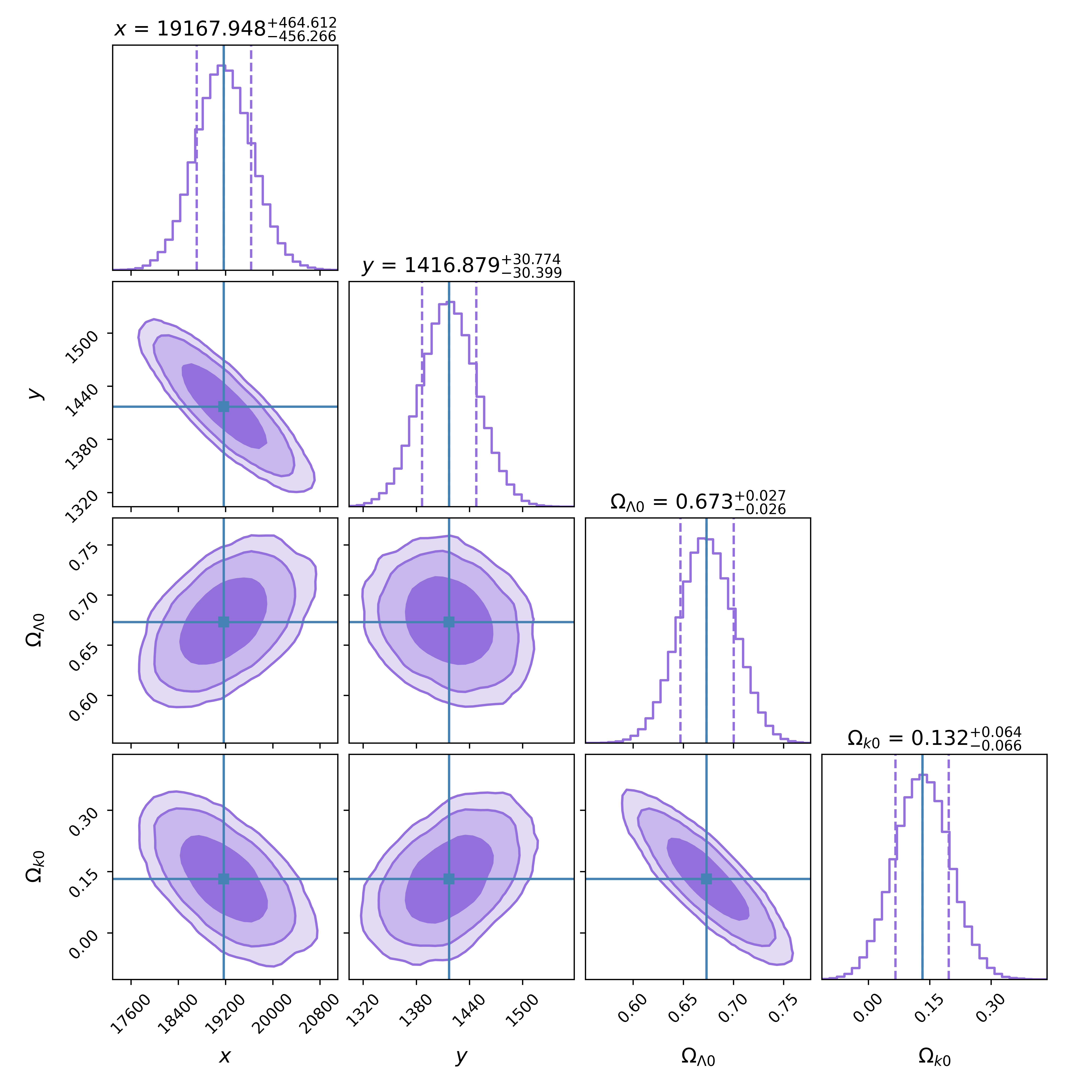
  Figure 3: As in Fig. 2, but for $n=2.5$.

• For $n=2.5$, a qualitative difference (as compared to the preceding cases) appears. $\Omega_{\Lambda}$ has moved to a value almost indistinguishable from that in the $\Lambda$CDM model, but with a relatively larger uncertainty (see Fig.3). On the other hand, there is strong preference (at over $2\sigma$) for a closed universe and $\Omega_{n0}$ has now switched signs! To appreciate this, note that $\Omega_{n}$ is now very unlike $\Omega_{\Lambda}$ and could, instead, be thought of being halfway between $\Omega_{k}$ and $\Omega_{m}$. Nominally, one would have expected a larger compensatory shift in $\Omega_{m0}$, but for the fact that the combination $y$ is rather strongly constrained. With this preventing $\Omega_{m0}$ from moving very substantially, $\Omega_{n0}$ can only be such that its effect on $H(z)$ could, to an extent, be compensated for by a non-zero $\Omega_{k0}$. Naturally, the correlations involving $\Omega_{k0}$ have now switched signs.

The excellent value of the reduced $\chi^{2}$ in each case is a testimony to the goodness of the fits, with very little to choose between them (see Fig.4).

IV Discussion and Conclusions

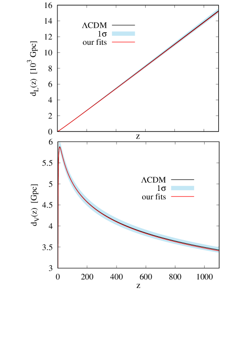
Figure 4: The cosmological distances $d_{L}(z)$ and $d_{V}(z)$ as a function of the red-shift $z$. Shown are the curves for $n=1$ (on the scale of the figures, the others are indistinguishable) as well as those for the $\Lambda$CDM model alongwith the uncertainties.

The $\Lambda$CDM model, while extraordinarily effective at explaining a wide spectrum of cosmological phenomena, is faced with mounting evidence of a ($\approx 5\sigma$) discrepancy between the measurements of the Hubble constant, $H_{0}$, made locally and that inferred from early universe observations. To address this ‘Hubble tension’, we propose a modified cosmological model with an additional ingredient whose energy density varies with redshift as $(1+z)^{n}$, where $n\in(0,3)$ is a discrete parameter determined by unknown physics.

The model is confronted with the Pantheon Compilation, which contains $1048$ data points from Type Ia Supernovae (SNe), and, simultaneously, required to be consistent with the $\Lambda$CDM model at redshift $z\approx 1100$. Regardless of the value of $n$, one of the key findings of the study is that a value of the present-epoch Hubble constant ($H_{0}$) consistent with the published value from the SH0ES survey, can also be rendered absolutely consistent with the PLANCK analysis.

At this stage, one must acknowledge that the PLANCK analysis is not the only one sensitive to physics in the early universe. Of increasing importance in this context are the studies of Baryon Acoustic Oscillations (BAO). The BAO data analysis incorporates the fitting of three cosmological distance measures, viz.,

$$\begin{array}[]{rcl}d_{H}(z)&\equiv&c/H(z)\\[4.30554pt] d_{A}(z)&\equiv&\left(1+z\right)^{-2}\,d_{L}(z)\\[4.30554pt] d_{V}(z)&\equiv&\left[z\,(1+z)^{2}\,d_{H}(z)\,d_{A}^{2}(z)\right]^{1/3}\end{array}$$ (7)

and our projections for these too must agree with the data, at least as well as the $\Lambda$CDM does.

Noting that $d_{A}$ and $d_{L}$ are essentially the same, and that $d_{H}$ can be obtained from $(d_{L},d_{V}$), in Fig. 4, we display this pair. Clearly, for each of the distance measures, our model (for all of the $n$ values) does as well as the $\Lambda$CDM. In other words, there is nothing to choose between them as far as the BAO data is concerned. This is not surprising, for our fitting did take into account both the low-$z$ and the CMBR data.

Bolstered by this finding, we now return to a recounting of the key findings. Scenarios with $n<2$ show a slight preference for an open universe with a cosmological constant that is decidedly smaller than that in the $\Lambda$CDM, with the two departures from the canonical scenario working opposite to each other at late times. However, it should be remembered that these scenarios are largely consistent with a vanishingly small $\Omega_{k0}$ and removing this component entirely would not substantially affect the fit. For $n>2$, however, a distinct preference for a closed universe is shown, the effect being most significant for $2.5\lesssim n\lesssim 2.75$ (with the system understandably reverting to $\Lambda$CDM as $n\to 3-$). This preference for a closed universe is not accompanied by an increase in $\Omega_{\Lambda}$ beyond the standard value (although the values are distinctly larger than those for $n<2$). Rather, the effect of the closure is partially compensated for by $\Omega_{n0}<0$, i.e., a negative energy density for the exotic matter! This invites a deeper analysis of its nature.

Last but not least, the 1D and 2D posterior contour graphs reveal weak correlations between the parameters. This implies that there may be subtle interdependencies among the modified model’s parameters and that additional research is required to completely comprehend the model’s behavior and pave the way for insight into the nature of dark energy and the expansion of the universe.

References

- Lemaitre (1927) G. Lemaitre, Annales Soc. Sci. Bruxelles A 47, 49 (1927).
- Hubble (1929) E. Hubble, Proc. Nat. Acad. Sci. 15, 168 (1929).
- Hinshaw et al. (2013) G. Hinshaw et al. (WMAP), Astrophys. J. Suppl. 208, 19 (2013), arXiv:1212.5226 [astro-ph.CO] .
- Aghanim et al. (2020) N. Aghanim et al. (Planck), Astron. Astrophys. 641, A6 (2020), [Erratum: Astron.Astrophys. 652, C4 (2021)], arXiv:1807.06209 [astro-ph.CO] .
- Scolnic et al. (2018) D. M. Scolnic et al. (Pan-STARRS1), Astrophys. J. 859, 101 (2018), arXiv:1710.00845 [astro-ph.CO] .
- Riess et al. (2022) A. G. Riess et al., Astrophys. J. Lett. 934, L7 (2022), arXiv:2112.04510 [astro-ph.CO] .
- Vagnozzi (2020) S. Vagnozzi, Phys. Rev. D 102, 023518 (2020), arXiv:1907.07569 [astro-ph.CO] .
- Trenti et al. (2015) M. Trenti, P. Padoan, and R. Jimenez, Astrophys. J. Lett. 808, L35 (2015), arXiv:1502.02670 [astro-ph.GA] .
- Jimenez et al. (2019) R. Jimenez et al., J. Cosmology Astropart. Phys. 2019, 043 (2019), arXiv:1902.07081 [astro-ph.CO] .
- Valcin et al. (2020) D. Valcin et al., J. Cosmology Astropart. Phys. 2020, 002 (2020), arXiv:2007.06594 [astro-ph.CO] .
- Bernal et al. (2021) J. L. Bernal et al., Phys. Rev. D 103, 103533 (2021), arXiv:2102.05066 [astro-ph.CO] .
- Boylan-Kolchin and Weisz (2021) M. Boylan-Kolchin and D. R. Weisz, Mon. Notices Royal Astron. Soc. 505, 2764 (2021), arXiv:2103.15825 [astro-ph.CO] .
- Bolte and Hogan (1995) M. Bolte and C. J. Hogan, Nature (London) 376, 399 (1995).
- Krauss and Turner (1995) L. M. Krauss and M. S. Turner, General Relativity and Gravitation 27, 1137 (1995), arXiv:astro-ph/9504003 [astro-ph] .
- Dunlop et al. (1996) J. Dunlop et al., Nature (London) 381, 581 (1996).
- Alcaniz and Lima (1999) J. S. Alcaniz and J. A. S. Lima, Astrophys. J. Lett. 521, L87 (1999), arXiv:astro-ph/9902298 [astro-ph] .
- Lima and Alcaniz (2000) J. A. S. Lima and J. S. Alcaniz, Mon. Notices Royal Astron. Soc. 317, 893 (2000), arXiv:astro-ph/0005441 [astro-ph] .
- Jimenez and Loeb (2002) R. Jimenez and A. Loeb, Astrophys. J. 573, 37 (2002), arXiv:astro-ph/0106145 [astro-ph] .
- Jimenez et al. (2003) R. Jimenez, L. Verde, T. Treu, and D. Stern, Astrophys. J. 593, 622 (2003), arXiv:astro-ph/0302560 [astro-ph] .
- Capozziello et al. (2004) S. Capozziello, V. F. Cardone, M. Funaro, and S. Andreon, Phys. Rev. D 70, 123501 (2004), arXiv:astro-ph/0410268 [astro-ph] .
- Friaça et al. (2005) A. C. S. Friaça, J. S. Alcaniz, and J. A. S. Lima, Mon. Notices Royal Astron. Soc. 362, 1295 (2005), arXiv:astro-ph/0504031 [astro-ph] .
- Jain and Dev (2006) D. Jain and A. Dev, Physics Letters B 633, 436 (2006), arXiv:astro-ph/0509212 [astro-ph] .
- Bengaly et al. (2014) C. A. P. Bengaly, M. A. Dantas, J. C. Carvalho, and J. S. Alcaniz, Astron. Astrophys. 561, A44 (2014), arXiv:1308.6230 [astro-ph.CO] .
- Wei et al. (2015) J.-J. Wei et al., Astron. J. 150, 35 (2015), arXiv:1505.07671 [astro-ph.CO] .
- Rana et al. (2017) A. Rana, D. Jain, S. Mahajan, and A. Mukherjee, J. Cosmology Astropart. Phys. 2017, 028 (2017), arXiv:1611.07196 [astro-ph.CO] .
- Nunes and Pacucci (2020) R. C. Nunes and F. Pacucci, Mon. Notices Royal Astron. Soc. 496, 888 (2020), arXiv:2006.01839 [astro-ph.CO] .
- Vagnozzi et al. (2021) S. Vagnozzi, A. Loeb, and M. Moresco, Astrophys. J. 908, 84 (2021), arXiv:2011.11645 [astro-ph.CO] .
- Di Valentino et al. (2021) E. Di Valentino et al., Class. Quant. Grav. 38, 153001 (2021), arXiv:2103.01183 [astro-ph.CO] .
- Kamionkowski and Riess (2022) M. Kamionkowski and A. G. Riess, arXiv e-prints , arXiv:2211.04492 (2022), arXiv:2211.04492 [astro-ph.CO] .
- Hu and Wang (2023) J.-P. Hu and F.-Y. Wang, Universe 9, 94 (2023), arXiv:2302.05709 [astro-ph.CO] .
- Nojiri and Odintsov (2007) S. Nojiri and S. D. Odintsov, Int. J. Geom. Methods Mod. Phys. 04, 115 (2007), arXiv:hep-th/0601213 [hep-th] .
- De Felice and Tsujikawa (2010) A. De Felice and S. Tsujikawa, Living Rev. Rel. 13, 3 (2010), arXiv:1002.4928 [gr-qc] .
- Capozziello and De Laurentis (2011) S. Capozziello and M. De Laurentis, Phys. Rept. 509, 167 (2011), arXiv:1108.6266 [gr-qc] .
- Cai et al. (2016) Y.-F. Cai, S. Capozziello, M. De Laurentis, and E. N. Saridakis, Rept. Prog. Phys. 79, 106901 (2016), arXiv:1511.07586 [gr-qc] .
- Carroll (2001) S. M. Carroll, Living Rev. Rel. 4, 1 (2001), arXiv:astro-ph/0004075 .
- Peebles and Ratra (2003) P. J. E. Peebles and B. Ratra, Rev. Mod. Phys. 75, 559 (2003), arXiv:astro-ph/0207347 .
- Copeland et al. (2006) E. J. Copeland, M. Sami, and S. Tsujikawa, Int. J. Mod. Phys. D 15, 1753 (2006), arXiv:hep-th/0603057 .
- Li et al. (2013) M. Li, X.-D. Li, S. Wang, and Y. Wang, Front. Phys. (Beijing) 8, 828 (2013), arXiv:1209.0922 [astro-ph.CO] .
- Tutusaus et al. (2019) I. Tutusaus, B. Lamine, and A. Blanchard, Astron. Astrophys. 625, A15 (2019), arXiv:1803.06197 [astro-ph.CO] .
- Kumar et al. (2022) D. Kumar et al., J. Cosmology Astropart. Phys. 2022, 053 (2022), arXiv:2107.04784 [astro-ph.CO] .
- Benevento et al. (2020) G. Benevento, W. Hu, and M. Raveri, Phys. Rev. D 101, 103517 (2020), arXiv:2002.11707 [astro-ph.CO] .
- Foreman-Mackey et al. (2013) D. Foreman-Mackey, D. W. Hogg, D. Lang, and J. Goodman, Publ. Astron. Soc. Pac. 125, 306 (2013), arXiv:1202.3665 [astro-ph.IM] .