A Quantitatively Interpretable Model for Alzheimer’s Disease Prediction using Deep Counterfactuals
Abstract
Deep learning (DL) for predicting Alzheimer’s disease (AD) has provided timely intervention in disease progression yet still demands attentive interpretability to explain how their DL models make definitive decisions. Recently, counterfactual reasoning has gained increasing attention in medical research because of its ability to provide a refined visual explanatory map. However, such visual explanatory maps based on visual inspection alone are insufficient unless we intuitively demonstrate their medical or neuroscientific validity via quantitative features. In this study, we synthesize the counterfactual-labeled structural MRIs using our proposed framework and transform it into a gray matter density map to measure its volumetric changes over the parcellated region of interest (ROI). We also devised a lightweight linear classifier to boost the effectiveness of constructed ROIs, promoted quantitative interpretation, and achieved comparable predictive performance to DL methods. Throughout this, our framework produces an “AD-relatedness index” for each ROI and offers an intuitive understanding of brain status for an individual patient and across patient groups with respect to AD progression.
Index Terms:
Alzheimer’s Disease, Counterfactual Reasoning, Quantitative Feature-Based Analysis, Counterfactual-Guided Attention1 Introduction
Alzheimer’s disease (AD) is a neurodegenerative brain disease characterized by memory loss, logical thinking difficulties, speech impairment, and problems with reading and writing [1]. Although many efforts have been made to enhance understanding and discover efficient treatment, the medication for AD is intended only to slow AD progression [2]. As numerous studies have revealed the advantages of early intervention [3], it is paramount to identify patients who have mild cognitive impairment (MCI)—a prodromal stage of AD that is likely to convert to AD [4]—to effectively delay cognitive decline. With advances in brain imaging techniques, such as structural magnetic resonance imaging (sMRI), a predictive framework that integrates clinical examination and imaging techniques [5] has been developed to understand brain disease-related structural changes. However, clinical examinations may vary contingent on which diagnosis index is used, as each includes various evaluation items. Thus, the visual inspection of such brain imaging scans inevitably depends on the qualitative evaluations and subjective decisions of radiologists and clinicians.
Originally derived from oncological studies [6, 7], radiomics has recently been used to extract quantitative features from brain imaging data to present objective and reliable disease-related characteristics and reflect anatomical landmarks. These quantitative features (e.g., density, volume, morphometry, and textures) have phenotypic characteristics beneficial for disease analysis [8]. Concurrently, quantitative feature-based machine learning (ML) techniques have been proposed as an essential component of computer-aided diagnosis and detection systems [9]. Unlike statistical methods [10, 11], which are based on group-level analysis, ML allows individual-level precise predictions for subjects [12] to recognize the intricate patterns of input features for downstream tasks. Although existing ML-based methods help identify MCI/AD at the individual-level, most of the biomarker region selection is biased toward a small set of pre-defined regions for the sake of validation alone [13]. That is, undiscovered disease-related regions are ignored, the regions that could feasibly be considered potential biomarkers. Moreover, obtaining sufficient reproducibility and generalizability over regions of interest (ROIs) used for assessment is challenging because the disease-relevant regions are manually predetermined [14, 11].
Deep learning (DL) [15] techniques have recently achieved impressive outcomes in the medical field and have made remarkable progress in 3D sMRI-based AD prediction than the conventional ML methods [16, 17, 18]. Having devised with a hierarchical structure, DL models are proficient in discovering informative patterns in a data-driven manner, which alleviates the need for an a priori handcrafted selection of disease-related regions by experts. Despite DL models significantly enhancing predictive performance, providing the underlying interpretable final decisions remains a longstanding goal. This unfavorable “black-box” nature of DL models impedes many studies from clearly explaining and interpreting how their proposed DL models make definitive decisions [19]. To resolve this issue, visual explanation-based approaches in the field of explainable artificial intelligence (XAI) [20] have increasingly been exploited for interpreting DL models for medical image analysis. Existing methods, such as attribution-based approaches [21, 22], offer the visual saliency map as explanatory evidence by analyzing the gradients or activations of the model. While such visual saliency maps can highlight the influences and contributions of the class-relevant features (e.g., particular disease-related ROIs) w.r.t the prediction in given input images, they tend to produce similar saliency maps across the wrong class labels, owing to an “attribution vanishing” problem [23].
Counterfactual reasoning has gradually emerged as an alternative because it can provide refined visual explanatory maps, called counterfactual maps (CF maps), which exhibit fundamental explanations regarding the model’s decisions in various hypothetical scenarios, similar to the human decision-making process [24]. Specifically, a CF map enables an observer to consider contrastive explanations and causal inference, such as why a particular decision is made instead of another, as well as observe how an alteration of specific attributes affects the model’s output [25]. Most preceding studies that yielded counterfactual reasoning in DL were built upon the generative adversarial network (GAN) [26] and its variants [27, 28, 29], thereby it is proficient at generating a potential outcome that reveals unobservable instances. In terms of MCI/AD prognosis, the generated CF map serves as a visual explanatory map that includes anatomical changes such as brain hypertrophies or atrophies, assuming that the cognitively normal (CN) is diagnosed as a patient (refer to Fig. 2(a)).
In practice, the shortcoming of such CF maps is that they still rely on visual inspection according to voxel-level morphometry such that these visual explanations are merely synthesized on the original images to understand the model’s decision. Similarly, most XAI-inferred medical imaging studies [29, 30, 17] generally provided a visual interpretation of predictive performance without properly proving their medical or neuroscientific validity. This issue limits the yielding of intuitive insights from a clinical perspective [31]. In practical application, exhibiting explanatory maps alone is not self-sufficient, nor do they fulfill an expectation to support MCI/AD prediction as clinically decisive auxiliary information. Thus, a key motivation for this study is to advance beyond the limitations of the DL-based visual explanatory in medical image analysis by making the insights derived from such methodologies more measurable, intuitive, and scalable to healthcare professionals, including radiologists and clinicians.
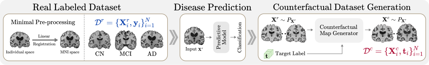
For these premises, we propose a novel framework for counterfactual-induced feature representation and quantitatively interpretable and explainable AD identification. As an extension of our prior study, we exploit LEAR’s counterfactual map generator (CMG) [29] to synthesize the counterfactual-labeled sMRI (c-sMRI) using the generated CF map via the given input (i.e., real-labeled sMRI, namely, r-sMRI), as depicted in Fig. 1(a). The newly produced c-sMRIs reflect the target counterfactual attributes with high confidence, so we employed the c-sMRIs as a disease-associated data augmentation set. By utilizing data-driven knowledge as augmented data, we can unlock a way to investigate the brain that has not yet been converted to the disease-manifested brain or even a clinically improbable case of reversed disease progression by producing alternative scenarios. We then transform both r-sMRIs and c-sMRIs into a gray matter (GM) density map (i.e., rGM and cGM) to precisely measure the volumetric changes in GM [32], associated with brain atrophies by aging [30] and AD progression [33, 34].
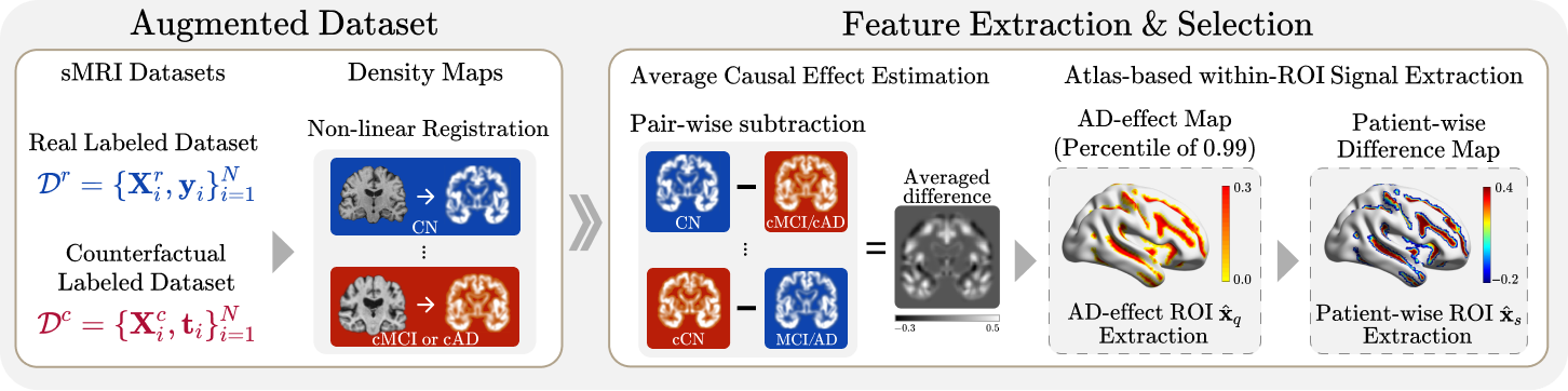
Given the rGM and cGM, we perform a series of GM density-based analyses (Fig. 1(b)) and assessments (Fig. 1(c)). First, we obtain the representative difference map by subtracting rGMs from their counterpart cGMs, followed by taking the first statistical moment (i.e., mean of difference maps). In this way, we estimate the so-called “average causal disease effect” (ACE) approximated by the difference in outcomes between the true (rGM) and the alternative scenario (cGM) from the same subjects. We refer to an estimated ACE as an AD-effect map, which portrays certain regions over the AD-affected anatomical variations within the AD spectrum. Subsequently, we explore the significant ROIs (i.e., AD-effect ROIs) by extracting prominent regions from the AD-effect map, such as the feature selection strategy. We further develop a shallow network of lightweight counterfactual-guided attentive feature representation and a linear classifier (LiCoL). Interestingly, the internal operation of the LiCoL from the input to the output can be rewritten as a linear function, as revealed in Supplementary H. This process helps interpret the counterfactual-guided attentive representation as the regional status of a brain, called an “AD-relatedness index”, and explains the output decision quantitatively based on the regional AD-relatedness index [35]. To our best knowledge, this work is the first sMRI-based AD prediction model that makes an input observation interpretable as a quantitative AD-relatedness index according to a DL-based visual explanation. Concretely, the main contributions of our study are summarized as follows:
-
•
We propose a novel methodology111Publicly available at https://github.com/ku-milab/LiCoL to develop fundamental scientific insights from a counterfactual reasoning-based explainable learning method. We demonstrate that our proposed method can interpret intuitively from the clinician’s perspective by converting counterfactual-guided deep features to the quantitative volumetric feature domain rather than directly inspecting DL-based visual attributions.
-
•
We achieved similar or better performance than DL models by designing a LiCoL with the AD-effect ROIs considered to be the distinctive AD-related landmarks via counterfactual-guided deep features.
-
•
By exploiting our proposed LiCoL, we provide a numerically interpretable AD-relatedness index for each patient as well as patient groups w.r.t anatomical variations caused by AD progression.
- •
2 Method
2.1 Counterfactual visual explanation model
In diagnosing clinical stages across the AD spectrum (i.e., CN/MCI/AD), the goal of the counterfactual visual explanation approach proposed in our LEAR [29] is to produce counterfactual reasoning for the decision of a predictive model (Fig. 1(a)). It consists of several key components: the counterfactual map generator (CMG), reasoning evaluator (RE), and discriminator (DC). Specifically, the CMG generates a CF map conditioned on an arbitrary target label, whereas the RE effectively guides the CMG toward comprehending the target label attributes in synthesizing realistic desired images. By exploiting the DC for carefully appraising the real and synthesized images (i.e., r-sMRIs and c-sMRIs ), the CMG will ascertain that the c-sMRIs are constrained as being realistic conversions. It should be noted that the RE is defined as the pre-trained predictive model , and the structure of the DC is identically imitated in the predictive model . Initially, we conducted pre-training for the predictive model (see Supplementary B) using supervised learning with training samples and one-hot encoded ground-truth labels :
| (1) |
where is a cross-entropy function. Henceforth, during the subsequent training phase to generate the CF maps, we fixed the weights of the RE while jointly tuning the trainable parameters of DC with the generator in CMG.
2.1.1 CMG architecture
The CMG is a variant of a conditional GAN [27] devised to effectively synthesize a CF map conditioned on a target label , where with denotes the size of the class distribution . Suppose that the c-sMRI can be induced through given an input , along with a target-specific CF map . The CMG shall be optimized in generating these maps such that the c-sMRI is diagnosed as the target label with high confidence. Specifically, the architecture of the CMG comprises the encoder and the generator , that is, a variant of U-Net [38] with a target label concatenated to the skip connections. Note that we replicate from the pre-trained predictive model in both its architecture and weights (fixed) so that adequately extracts the class-relevant features from .
As the CMG should consider the target label to produce the CF map, we fuse the target-specific characteristics onto the feature maps obtained from the encoder via a concatenation operation. For this purpose, we tile the target label to match the shape corresponding to the respective feature maps of the -th convolution layer. To obtain the hierarchical discriminative representations w.r.t the target label, we devise an additional module that comprises a convolution operation (Conv3D) with a trainable kernel, a stride of one in each dimension, and zero padding, followed by a Leaky-ReLU activation function ():
| (2) |
where denotes an operator of channel-wise concatenation, and denote the output feature maps of the convolution layers from the encoder . Subsequently, the target-fused feature maps are transferred to the generator via skip connections. The generator is then capable of seamlessly generating a CF map from the target label-informed feature maps:
| (3) |
where . Lastly, we produce a c-sMRI by incorporating the CF map with an input using addition, i.e., , which is supposed to be diagnosed as the target label .
2.1.2 The objective function of the CMG
To generate a realistic c-sMRI , we adopt the least square GAN (LSGAN) [39] loss function to enforce a stable optimization by penalizing samples far from the DC’s decision boundary. Guided by this loss, the DC assists the CMG such that it will thoughtfully minimize the substantial distance between the real and generated distributions:
| (4) | ||||
| (5) | ||||
where and denote the c-sMRI and its respective override c-sMRI (will also be utilized for cycle consistency), respectively, and denotes the distribution of r-sMRI samples. Note that indicates the CF map overriding the c-sMRI to obtain which is expectedly to resemble the r-sMRI conditioned by .
Because the DC is employed merely to differentiate between the input and the generated and , it does not have the immediate capacity to explicitly guide the CMG to either preserve the appearance of the input or endorse the target attribution during the generative process. Thus, we employ a cycle consistency loss [40] based on the -norm to produce enhanced target-dependent CF maps. In this way, we force the CMG to consistently strive for various conditions without suffering from a mode collapse [26]:
| (6) |
where denotes the one-hot encoded vector drawn randomly from a discrete uniform distribution.
Furthermore, we utilize the total variation loss to reconcile the elaborate synthesis between the input and its CF map . In particular, total variation loss ensures that the c-sMRI imposes local spatial continuity and smoothness to mitigate unnatural and overly pixelated results, which encourages visual coherence in a real image:
| (7) | ||||
where and , , and are the 3D coordinates of each index in volumetric images.
Elastic regularization is also applied to the CMG to impose a constraint on the magnitude of the CF map . By doing this, the vast majority of fine-grained feature attributions for counterfactual reasoning are highlighted such that minimal modifications over the features induce a converted prediction from to the target .
| (8) |
where and are weighting constants.
As adequate assistance to the generator , we employ the classification loss function to produce CF maps that transform an input so that it is precisely classified as a target label :
| (9) |
Consequently, we define the composite objective function for the overall CF map generation task as follows:
| (10) |
where values are the hyperparameters for model training. We empirically tune such that the magnitudes of the gradients for each loss term are roughly balanced.
2.2 Quantifying explainability of counterfactual-guided deep features
Having sufficiently optimized the CF map generation task, we extend our work [29] in quantifying the explainability of the acquired counterfactual-guided deep features in terms of AD prediction. For this purpose, we carefully devise the overall explainability quantification steps, including (i) establishment of image manipulation, (ii) extraction of AD-related landmarks, and finally (iii) usage of a lightweight counterfactual-guided attentive feature representation and a linear classifier (LiCoL). The procedures of this in-depth analysis are depicted in Fig. 1(b) and Fig. 1(c).
2.2.1 Establishment of image manipulation
This brain image manipulation step aims to establish a proportional approach to quantify the explainability of deep features as a gray matter (GM) density map. The utilization of a GM density map assists in conducting accurate numerical measurements and quantitative feature-based analysis of brain disease. To this end, we devise subsequent procedures to reverse the process used for acquiring the train-ready input (i.e., r-sMRIs) from a raw brain image . In this way, the GM density map, including counterfactual-guided deep features, is obtained by manipulating the reflective superimposed processing.
Specifically, both r-sMRI and the corresponding c-sMRI are fed into a series of reverse preprocessing steps consisting of reverse Gaussian normalization, reverse quantile normalization, and up-scaling steps. To calculate the reverse Gaussian normalization, each mean and standard deviation of the subject is stored during preprocessing and reused to recover the original values. The subsequent step is reverse quantile normalization; however, it is intractable to process the c-sMRI by simply reversing the quantile normalization, as opposed to r-sMRI . Since the previous values of voxels where normalization was performed by quantile thresholding are unknown after synthesizing with a CF map, we resort to a histogram-matching technique as a surrogate solution. By viewing the model’s input as an alternative ground truth, which is paired with the being processed, we adequately circumvent this issue through the alignment of quantile-normalized voxels. Thereafter, the final reversed raw image is acquired using an up-scaling operation to match the size of (i.e., ).
Furthermore, a few auxiliary steps are carried out to produce the GM density map over a set. There are four kinds of steps: (i) as the was skull-stripped and linearly registered into MNI152 space, those images are instantly segmented into GM, white matter, and cerebrospinal fluid volume probability maps using FMRIB’s automated segmentation tool [41], (ii) segmented GM images are nonlinearly registered using FMRIB’s nonlinear registration tool to generate GM density maps for each image, (iii) we then modulated these GM density maps via Jacobian of the warp field, (iv) the resulting GM density maps are finally smoothed with an isotropic Gaussian kernel with a of 2 mm for alleviating contrast and other irrelevant details. It should be noted that values in acquired GM density maps refer to the intensity of GM density within the brain regions.
2.2.2 Extraction of AD-related landmarks
Given a set of manipulated GM density maps, we further investigate the validity of counterfactual-guided deep features, applying the average causal disease effect for GM density-based analysis. Let and denote the rGM and the cGM manipulated via an r-sMRI and the c-sMRI , respectively. We first subtract rGMs from their corresponding cGMs in diverse clinical stages to acquire the stage-wise difference maps. For instance, for a CN-labeled rGM, the counterpart of its clinical label for the cGM shall be defined as the AD or MCI, depending on the given scenario. The favorable properties of difference maps encompass a discriminative capability to prominently reflect inherent disease-associated regional localization as well as the unique anatomical characteristics between the different disease-state groups. These difference maps are then averaged into a representative difference map, which refers to as the AD-effect map , by exploiting the first moment in statistics (i.e., the mean of difference maps) as:
| (11) |
where and denote the total number of samples and the absolute operation, respectively. Note that the purpose of applying an absolute operation is to emphasize areas where the magnitude of GM density alterations between clinical stage groups are prominent, considering the variability of AD-sensitive regions. Such an AD-effect map is finally masked by the percentile threshold that reveals the most distinctly highlighted regions among the set of fine-grained regions (illustrated in Fig. 1(b)).
2.2.3 AD-effect ROI composition
Brain parcellation not only provides an understanding of the fundamental brain organization and function of closely interacting regions but also compresses information from hundreds of thousands of voxels or vertices into manageable sets. Under these characteristics, we adopt an ROI-based analysis that extracts and analyzes significant ROIs across voxel-level values, which are residing on the AD-effect map . To this end, the automated anatomical labeling (AAL3) atlas [42] (see Supplementary G) is overlaid on the AD-effect map to further subdivide it into individual regions, so that each trimmed region is completely within the cortical and subcortical regions and has anatomical specificity. We utilize a set of voxel indices across the parcellated regions to aggregate the region-wise highlighted voxels on the AD-effect map with a thresholding parameter (see Supplementary C and Supplementary J). We then take the average over the total number of highlighted voxels in each region. Eventually, representative ROIs are defined by concatenating the region-wise aggregated values as:
| (12) |
Here, and denote the operator of concatenation and the total number of adopted parcellated regions, respectively, while denoting as the indicator function that returns 1 if the given condition is true, or returns 0 otherwise. We define as the count of elements in a given argument; thereby, denotes the total number of voxel indices within -th parcellated regions. With this, we obtain the significant ROI as AD-effect ROIs, which consist of number of ROIs as .
2.2.4 LiCoL architecture
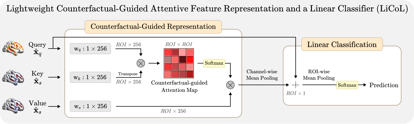
We perform an objective classification task to verify the effectiveness of the acquired AD-effect ROIs . Inspired by Transformer [43], which could consider the global relationship, we devise a LiCoL to quantitatively account for the most influential ROIs, which contributed to the AD prediction among AD-effect ROIs (illustrated in Fig. 1(c)).
In a nutshell, our proposed LiCoL maps a set of ROIs (i.e., the type of vector) comprised of query, key, and value onto the input. As AD-effect ROIs contain the characteristics of universal subregions where GM density differences between clinical stages are prominent concerning AD progression, we establish the query as AD-effect ROIs to adequately guide the attention within the LiCoL. Contrary to the query, the key and value are individually constructed for each training sample. Similar to AD-effect ROI acquisition in Eq. (12), the key and value would be defined as patient-wise ROIs , which have averaged the voxel values corresponding to the voxel indices in each GM density map along the parcellated region. Subsequently, the query, key, and value are transformed into the set of embedded matrices by multiplying ROIs with the respective embedding layer . Specifically, the set of represent the embedded matrices produced from a linear transformation, , , and , respectively, where and are learnable embedding weights. We then compute the counterfactual-guided attention matrix as:
| (13) |
where and respectively denote a transpose operation, and the number of ROIs used from the key for scaling, while denotes the softmax function. Through Eq. (13), our LiCoL allows for enforcing the predominant difference between clinical stages (i.e., inter-subject variability) while reflecting the discriminative attributes of the patient’s individual (i.e., intra-subject variability).
To infer the diagnostic prediction, we first apply the channel-wise mean pooling to reshape the output of the counterfactual-guided attention map to match the same size as the input query , so that the size of the counterfactual-guided attention map pooled in the channel is defined as . Thereafter, we employ a residual connection using an element-wise addition, followed by an ROI-wise mean pooling to obtain the final predicted label as the following:
| (14) |
where denotes the softmax function.
Eventually, we train the LiCoL by minimizing the classification loss via as:
| (15) |
where and denote a GM density map and its ground-truth label, respectively. It should be noted that during training, the LiCoL is learned employing both rGMs and cGMs, but it uses only test samples acquired from the rGMs to evaluate the performance of the LiCoL.
3 Results and Analyses
3.1 Datasets
The ADNI and GARD comprised 3D sMRIs and were acquired from various patient groups ranging from those with CN to those with MCI and AD. These three categories were annotated based on the standard clinical criteria, including mini-mental state examination (MMSE) scores and clinical dementia ratings. Although some subjects had accumulated multiple MRIs through their follow-up in both datasets, we only selected and utilized their baseline (first-visit) MRIs. The sMRI preprocessing and details of the subjects’ demographic information are summarized in Supplementary A.
The ADNI dataset consisted of 1,540 sMRI scans that included CN subjects (n = 433), MCI subjects (n = 748), and AD subjects (n = 359) from the combined ADNI-1 and ADNI-2 studies. As a special case for ADNI, two subgroups of MCI subjects were sampled: the progressive MCI (pMCI) (n = 251), including MCI subjects who converted to AD within 36 months of screening, and the stable MCI (sMCI) (n = 497), including those who remained in the MCI group within 36 months of screening. The baseline of the ADNI-1 included 1.5T T1-weighted sMRI scans acquired from 822 subjects, and ADNI-2 included 3T T1-weighted sMRI scans acquired from 718 subjects. Meanwhile, the baseline GARD dataset contained 1.5T T1-weighted sMRI scans acquired from 745 subjects, including CN subjects (n = 261), MCI subjects (n = 375), and AD subjects (n = 109).
3.2 Experimental setup
As the ADNI dataset consists of four categories (i.e., CN, sMCI, pMCI, and AD), we merged the subjects of the sMCI and pMCI as MCI to maintain consistency with the GARD dataset. Henceforth, we evaluated both datasets for four scenarios: (i) CN MCI, (ii) MCI AD, (iii) CN AD, and (iv) CN MCI AD. We further performed the CN sMCI pMCI AD scenario using the ADNI apart from the granularity issues of GARD and reported their results in Table S19 and Table S20. All experiments and evaluations were conducted using five-fold cross-validation.
3.2.1 Evaluation metrics
All experimental results for the predictive performance were quantitatively validated and evaluated using four criteria: the (multi-class) area under the receiver operating characteristic curve (mAUC or AUC), accuracy, sensitivity, and specificity. Specifically, the best predictive model for generating counterfactual images was selected by assessing the AUC during training, and the test performance corresponding to its model was reported in Supplementary B. Meanwhile, we further measured the predictive performance under these evaluation metrics to verify the effectiveness of our proposed LiCoL along with AD-effect ROIs. To affirm the generalizability of the cGM for augmentation, we used precision and recall, which were preferred over other alternatives when the class distribution was significantly skewed [44].
3.2.2 Statistical hypothesis test
For the AD-effect map acquisition and augmentation of cGMs for the statistical map, we measured the statistical significance of categorizing with the same population using a two-sample t-test (-value 0.05) to group the same clinical stage of the rGMs and cGMs. This statistical test indicates that two independent samples have identical expected values. Thus, it can be assumed that the cGMs are adequately mapped on the identical distribution of rGMs, respectively. In a nutshell, the AD-labeled cGM and the AD-labeled rGM were considered the same AD category.
3.3 Verification of counterfactual images
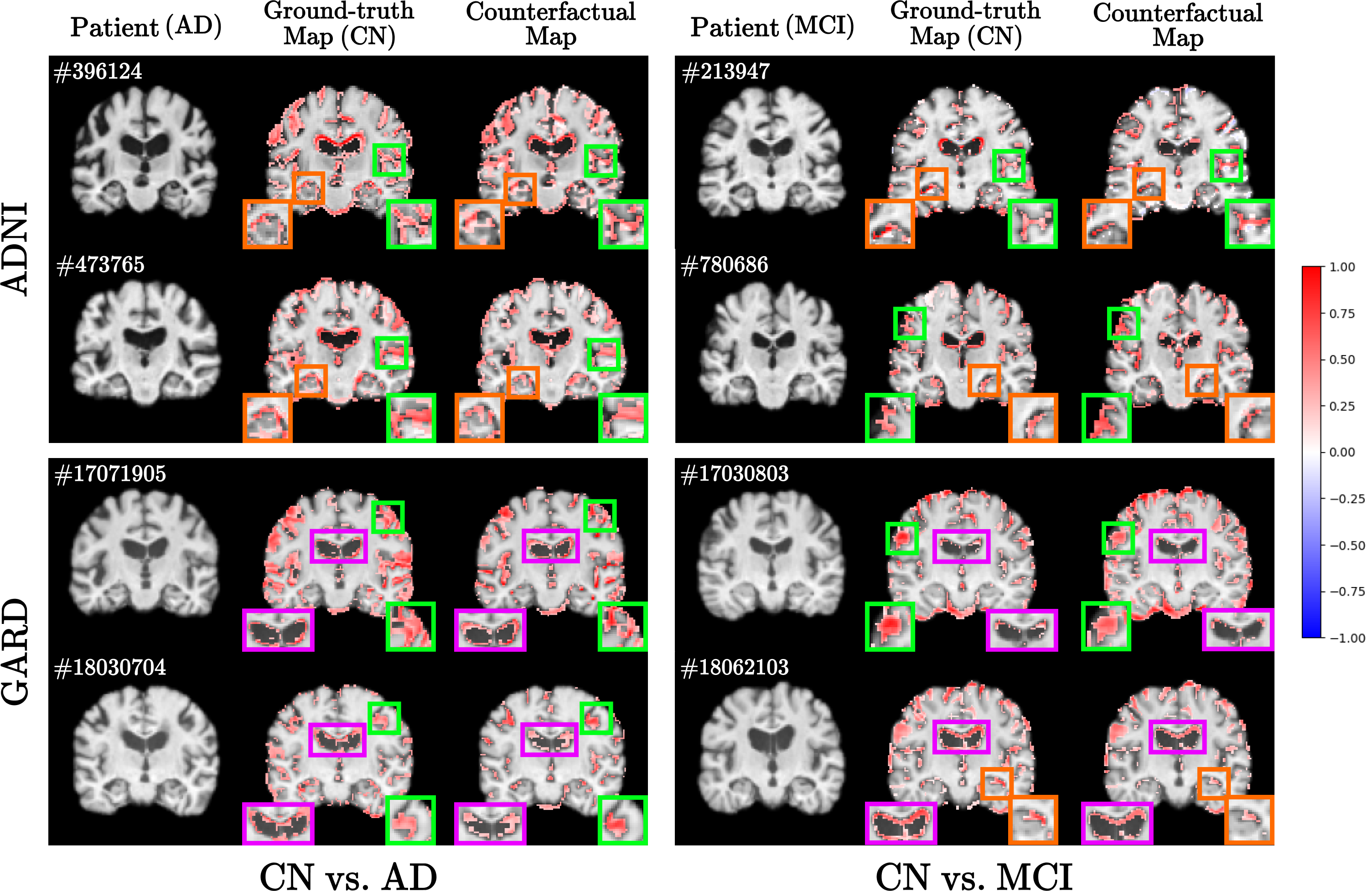
We conducted qualitative and quantitative assessments to validate the reliability of counterfactual reasoning on the ADNI and GARD datasets. As no ground truth is available to evaluate the generated CF map, we constructed the “pseudo” ground-truth map (i.e., an observed disease progression map), defined as the difference between longitudinal samples of two different clinical stages over the same patient (refer to Supplementary D). For example, if the CN subject is selected as a baseline, either the MCI or AD subject shall be defined as a counterpart of the target image, depending on the scenario. This ground-truth map (second column in each scenario of Fig. 2(a)) exhibited an excellent representation of atrophies, indicating which regions were changed according to the clinical stage conversion.
In Fig. 2(a), we illustrate the CF map examples generated by our CMG [29] from the tasks of CN AD and CN MCI classification. The generated CF maps on both the ADNI and GARD longitudinal samples showed excellent agreement with their corresponding pseudo-ground-truth map. In fact, the hippocampal region (orange box) is known to be the most prominent MCI/AD region [14, 45]; however, it is also known that morphological variations due to MCI/AD in many other regions are also involved. Regarding these disease characteristics in the brain, we observed that our CMG successfully captured reduced ventricle and hypertrophy in the hippocampus [46] while containing subtle variations that occurred in most cerebral cortex regions.
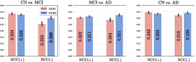
As a numerical assessment metric of the generated CF maps, we calculated the NCC score in Fig. 2(b) to measure the morphological and structural similarity between a generated CF map and a pseudo-ground-truth map as proposed by [29]. We leveraged the NCC score because it has the primary property of not being sensitive to the magnitude of the signals. Compared with the LEAR’s performance [29], which reported the ADNI performance only, the NCC scores of GARD were comparable to those on the ADNI in all scenarios. Based on these NCC scores, we hypothesized that the generated CF maps on both ADNI and GARD datasets captured pathologically subtle changes associated with AD progression, yielding the CMG’s scalability over two independent and different racial data sources. As an extensive analysis, we further experimented with the cross-domain scheme across the ADNI and GARD in Supplementary B and compared the accuracy of the CMG when precisely predicting the synthesized images as the target label in Supplementary I. In addition, we have thoroughly conducted ablation studies of an entire pipeline according to the losses used in the CMG training to quantitatively and qualitatively explore how the quality of synthesized images influences classification performance in Supplementary J. Leveraged by those qualitatively and quantitatively promising results, we can justify our proposed framework to exploit the counterfactually-generated samples and accept our findings from the experimental analysis described below.
3.4 AD-effect map and ROI feature representation
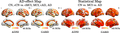
Using Eq. (11), we estimated AD-effect maps for binary scenarios that identify cortical and subcortical brain regions, where the GM density contrasts were considerably differentiated between clinical stages (results of AD-effect maps in Fig. 3). Similar to the ensemble strategy, we gathered the rGMs and cGMs used in each binary scenario to generate AD-effect maps over the multi-class scenario. Subsequently, we partitioned them into normal (i.e., CN, cCN) and patient (i.e., cMCI, MCI, cAD, AD) groups and calculated the AD-effect map via Eq. (11) in the same way as in binary scenarios (see Fig. 4). By doing so, this map is possible to fully cover the disease progression across the AD spectrum. In particular, the merit of this strategy is to incorporate the outcomes of each binary scenario, which can focus on distinguishing between specific pairs of classes, allowing it to specialize in maximizing the discriminative power between those classes, potentially improving accuracy for distinguishing specific disease heterogeneity. For comparison, we computed a conventional group-level statistical map (-value 0.01) by measuring the two-sample t-test between different stages of rGMs for binary scenarios and ANOVA among all disease stages of rGMs for multi-class scenarios (results of statistical maps in Fig. 3 and Fig. 4). Note that the AD-effect map and statistical map used a 0.99 percentile threshold and -value 0.01, respectively, which showed the highest validation performance across all scenarios (see Table S13).

Regarding feature engineering, we considered these AD-effect and statistical maps to identify the class-discriminative areas and applied different thresholding strategies (i.e., percentile -value) for ROI selection. For the configuration of statistical ROIs , we used Eq. (12), substituted from the AD-effect map to the statistical map. Although such AD-effect and statistical ROIs are produced at the equivalent criterion, the fundamental disparity in acquiring significant ROIs is provoked by each property underlying the AD-effect map and statistical map. The AD-effect map aims to discern regions of the brain with atrophy and hypertrophy that are the most drastically activated, whereas the statistical map takes into account the probability of observing a difference in disease progression.
In Fig. 3 and Fig. 4, the AD-effect map showed a more fine-grained regional localization than the statistical map. Whereas some areas were identically prominent in the AD-effect and statistical maps, other regions were revealed by only one map. Based on the classification performance in Table S13, we assume that the AD-effect map has better-localized regions than the statistical map. On the one hand, the statistically significant areas do not necessarily reflect class-discriminative information at an individual-level prediction. On the other hand, our proposed AD-effect map finds class-discriminative areas, which may not be statistically significant in a size-limited dataset by distilling the augmented cGMs. Intriguingly, according to the scenario in which the disease progressed from CN to AD, the number of AD-effect ROI and statistical ROI showed a tendency to increase gradually. One possible explanation for such differences is the clinical heterogeneity between MCI and AD based on disease severity. This could be supported by our observation that the MCI group in both ADNI and GARD datasets had fewer significant ROIs in the CN MCI scenario, despite having a larger amount of samples than the AD group (see Table S1). Therefore, we hypothesize that this scenario would have resulted in fewer ROIs because of the difficulty in highlighting the dementia-manifested regions within CN and MCI owing to anatomically subtle variations. The effectiveness and thorough analysis of these significant ROIs are described in the following subsections.
3.5 Predictive performance evaluation
We performed exhaustive experiments on the predictive performance of our proposed LiCoL and the effectiveness of the AD-effect ROI set . As competing methods, we have adopted ML- and DL-based models, which possessed inherent interpretability for the model’s decision or achieved state-of-the-art AD classification performance. Refer to Supplementary C for the implementation details and hyperparameters for baselines and our LiCoL training.
| ADNI | GARD | |||||||||
|---|---|---|---|---|---|---|---|---|---|---|
| Model | Params | AUC | Accuracy | Sensitivity | Specificity | AUC | Accuracy | Sensitivity | Specificity | |
| CN MCI | SVM | - | 0.67210.02∗∗ | 0.68820.03∗∗ | 0.66550.03 | 0.73850.01 | 0.71450.02∗∗ | 0.70590.03∗∗ | 0.72810.05 | 0.67980.03 |
| ResNet18 | 33.17M | 0.71780.03∗ | 0.71640.02∗ | 0.72150.05 | 0.69760.04 | 0.73950.03∗ | 0.72110.03∗ | 0.73850.05 | 0.76610.04 | |
| ResAttNet | 64.13M | 0.73450.03 | 0.72590.03 | 0.74890.02 | 0.73980.02 | 0.76580.02 | 0.76210.03 | 0.72850.04 | 0.80130.02 | |
| ViT | 33.87M | 0.70710.06∗∗ | 0.71190.06∗ | 0.69850.04 | 0.74810.05 | 0.71530.04∗∗ | 0.72180.04∗ | 0.69870.05 | 0.74360.04 | |
| M3T | 29.12M | 0.74530.03 | 0.73890.03 | 0.72740.05 | 0.77480.04 | 0.76980.03 | 0.76570.03 | 0.73150.04 | 0.83040.04 | |
| DSTANet | 3.04M | 0.75920.03 | 0.74480.02 | 0.70930.05 | 0.81420.04 | 0.77580.04 | 0.76900.03 | 0.74080.05 | 0.81890.04 | |
| LiCoL | 1,536 | 0.76780.01 | 0.75620.02 | 0.71430.02 | 0.81820.02 | 0.77780.02 | 0.76620.02 | 0.74850.03 | 0.82460.02 | |
| MCI AD | SVM | - | 0.75190.01∗ | 0.73290.02∗ | 0.66570.03 | 0.77850.03 | 0.72840.03∗ | 0.73860.03∗ | 0.83290.04 | 0.73910.04 |
| ResNet18 | 33.17M | 0.77050.01 | 0.75510.04∗ | 0.69710.06 | 0.84950.05 | 0.75690.03∗ | 0.77290.04 | 0.66190.04 | 0.81830.05 | |
| ResAttNet | 64.13M | 0.77190.03 | 0.78950.02 | 0.78140.03 | 0.88240.03 | 0.77190.03 | 0.79320.02 | 0.69180.06 | 0.80960.03 | |
| ViT | 33.87M | 0.74580.06∗ | 0.71790.05∗∗ | 0.63210.11 | 0.81950.13 | 0.73920.06∗ | 0.73280.04∗ | 0.70890.07 | 0.81340.08 | |
| M3T | 29.12M | 0.77880.03 | 0.79030.04 | 0.79890.05 | 0.88870.04 | 0.78110.04 | 0.77950.03 | 0.73950.05 | 0.79420.04 | |
| DSTANet | 3.04M | 0.76860.03 | 0.78690.04 | 0.77590.05 | 0.89810.03 | 0.76980.04 | 0.77710.03 | 0.86590.04 | 0.79270.03 | |
| LiCoL | 1,536 | 0.77270.02 | 0.79210.02 | 0.80140.02 | 0.89130.02 | 0.77530.02 | 0.78140.02 | 0.89170.01 | 0.79550.02 | |
| CN AD | SVM | - | 0.91670.01 | 0.91670.01 | 0.88890.02 | 0.94440.02 | 0.87740.02∗∗ | 0.85330.03∗∗ | 0.89120.02 | 0.87780.01 |
| ResNet18 | 33.17M | 0.92650.03 | 0.92190.04 | 0.90780.03 | 0.92090.05 | 0.89300.03∗ | 0.89130.03 | 0.87330.05 | 0.90930.04 | |
| ResAttNet | 64.13M | 0.92670.01 | 0.91860.02 | 0.88890.03 | 0.95440.03 | 0.92540.02 | 0.91170.02 | 0.91680.02 | 0.91690.03 | |
| ViT | 33.87M | 0.91870.07 | 0.91830.04 | 0.89700.05 | 0.94150.06 | 0.90520.04 | 0.91030.03 | 0.93140.04 | 0.89210.05 | |
| M3T | 29.12M | 0.93440.03 | 0.93010.04 | 0.93110.03 | 0.95690.03 | 0.92790.03 | 0.92150.02 | 0.90320.04 | 0.94330.02 | |
| DSTANet | 3.04M | 0.92860.03 | 0.92370.03 | 0.91850.04 | 0.95330.04 | 0.92710.04 | 0.91370.02 | 0.92870.04 | 0.89680.06 | |
| LiCoL | 1,536 | 0.93710.01 | 0.92850.01 | 0.92710.02 | 0.95910.02 | 0.93040.01 | 0.91930.01 | 0.94410.01 | 0.92830.01 | |
3.5.1 Quantitative comparison with ML methods
We employed six ML models, i.e., support vector machine (SVM), random forest, logistic regression, decision tree, Lasso regression, and Ridge regression. Table I and Table II present the results of SVM, as it achieves the best performance among the comparative ML baselines222The other ML baselines’ performance using and is reported in Table S14, Table S15, and Table S17, respectively.. Note that the SVM performance reported in these tables represents the results trained with for a fair comparison with our LiCoL. Nonetheless, our method outperformed the mean AUC (ADNI: 4.56% and GARD: 5.44%) and mean accuracy (ADNI: 4.63% and GARD: 5.64%) of SVM in all binary scenarios with statistical significance. In addition, even in the multi-class scenario, our LiCoL has still shown outstanding performance in mAUC (ADNI: 4.62% and GARD: 4.75%) and accuracy (ADNI: 3.40% and GARD: 3.39%) over SVM. Most remarkably, utilizing achieved better performance improvement in the CN MCI and the CN MCI AD scenario compared to performance (refer to Table S14, Table S15, and Table S17), despite being difficult to identify disease-affected regions associated with brain atrophies owing to subtle anatomical variations. Having observed these predictive outcomes, we confirmed that our discovered played a critical role in revealing a relatively substantial difference in GM density. Thus, this piece of evidence assisted in exploiting because of its promise to distinguish most class-discriminative regions.
| ADNI | GARD | ||||
|---|---|---|---|---|---|
| CN MCI AD | Model | mAUC | Accuracy | mAUC | Accuracy |
| SVM | 0.73570.03∗ | 0.61060.05∗ | 0.75320.03 | 0.62350.05 | |
| ResNet18 | 0.71530.05∗∗ | 0.57290.08∗∗ | 0.72480.06∗ | 0.58230.07∗∗ | |
| ResAttNet | 0.72320.04∗∗ | 0.60960.05∗ | 0.73130.05∗ | 0.60370.06∗ | |
| ViT | 0.72580.04∗ | 0.60170.03∗ | 0.72780.04∗ | 0.59730.04∗ | |
| M3T | 0.75480.04 | 0.62860.04 | 0.76120.04 | 0.63170.05 | |
| DSTANet | 0.77840.04 | 0.64880.03 | 0.78590.03 | 0.65380.05 | |
| LiCoL | 0.79190.03 | 0.66810.04 | 0.79720.04 | 0.66740.04 | |
| Scenarios | Data | ROIs | Categories | ||
|---|---|---|---|---|---|
| Baseline | Intersection | Union | |||
| CN MCI | ADNI | 0.72220.02 | 0.72840.01 | 0.73890.03 | |
| Ours | 0.76780.01 | 0.74820.03 | 0.76040.02 | ||
| GARD | 0.73850.02 | 0.74560.02 | 0.74790.02 | ||
| Ours | 0.77780.02 | 0.75920.02 | 0.77450.03 | ||
| MCI AD | ADNI | 0.75140.02 | 0.75380.02 | 0.76850.03 | |
| Ours | 0.77270.02 | 0.77270.02 | 0.76940.02 | ||
| GARD | 0.74970.04 | 0.75120.03 | 0.75810.03 | ||
| Ours | 0.77530.02 | 0.76930.01 | 0.77370.02 | ||
| CN AD | ADNI | 0.89120.02 | 0.89330.01 | 0.91460.01 | |
| Ours | 0.93710.01 | 0.93710.01 | 0.93080.02 | ||
| GARD | 0.90130.01 | 0.90740.01 | 0.92110.01 | ||
| Ours | 0.93040.01 | 0.93040.01 | 0.92770.02 | ||
| CN MCI AD | ADNI | 0.72870.04 | 0.72390.03 | 0.73090.03 | |
| Ours | 0.79190.03 | 0.78470.03 | 0.77130.04 | ||
| GARD | 0.73380.03 | 0.73380.03 | 0.74050.03 | ||
| Ours | 0.79720.04 | 0.78580.04 | 0.76810.04 | ||
3.5.2 Quantitative comparison with DL methods
As for the DL baselines, we adopted CNN-based [47, 17] and Transformer-based [48, 49, 50] methods, including ResNet18 [47], ResAttNet [17], ViT [48], M3T [49], and DSTANet [50]. ResNet18 [47] is known as a CNN-based representative image classifier and a model that derives superior performance in various prediction tasks. ResAttNet [17] is a variant of the ResNet that combines the internal self-attention modules. ViT [48] is a series of Transformers that deals with image patches as a sequential input. M3T [49] synergically models the integration of CNN and Transformer architectures and exploits various 2D views (i.e., multi-planes and slices) from 3D MRIs. DSTANet [50] is designed by the Transformer that replaces dot-product attention to diffusion kernel attention while utilizing brain ROIs as an input sequence, similar to our LiCoL. In Table I and Table II, the results of all DL baselines were also distilled with cGMs for a fair assessment, and the strategy of cGM augmentation resulted in notable performance improvements on all DL baselines when comparing to without augmenting the cGMs (refer to Table S16 and Table S18). Interestingly, comparative methods based on sequential modeling generally performed better in all scenarios, whereas ViT derived relatively lower performance than pure ResNet and other DL baselines. We conjectured such varying trends might be due to the lack of training samples, as ViT requires large samples for representation learning.
It is noteworthy that, albeit a lightweight classifier, LiCoL derived performance on par with DL baselines across all binary scenarios and achieved state-of-the-art performance in the multi-class scenario. In particular, DL models are built on layers of networks using complex non-linearity with numerous learning parameters, yielding high classification performance yet inevitably sacrificing interpretability. Contrarily, we designed the LiCoL with linearity so that the internal representations could be interpretable, such as other conventional ML models. Accordingly, the rationale behind any classification decision was straightforward to understand without additional tools or computations.
3.6 Discrepant ROIs analysis between AD-effect and statistical ROIs
We further investigated the variability in (m)AUC performance when using common or additive discrepant ROIs (i.e., ) and discrepant ROIs (i.e., ). To evaluate the validity of those ROIs, we separated the set of ROIs into three categories: (i) baseline ( and ), (ii) intersection (), and (iii) union ( or ). Here, we re-trained our LiCoL as a classifier according to each ROI combination. As revealed in Table III, the best predictive performance was achieved by the model that used the baseline . We also presented the results of using intersection and union derived from the (Ours), revealing a slightly decreasing tendency compared with the baseline in several scenarios. That is, could be regarded as ROIs that would not significantly contribute to the improvement of predictive performance despite showing statistical significance. Meanwhile, the union with in all scenarios exhibited an average (m)AUC performance improvement (ADNI: 1.49% and GARD: 1.11%) over baseline. We thus believe that utilizing discrepant ROIs contributed to enhanced predictive scores as they only reflect the distinct differential regions among disease-related variations resulting from disease progression. In this light, could be elucidated as potential biomarkers that have not appeared in the statistical test but were substantial.
From the comprehensive results, we investigated two instances over the and intersection ROIs that were revealed across all scenarios of both ADNI and GARD. The intersection ROIs were L.PreCG, L/R.SFG, L/R.MFG, L.IFGtriang, L.REC, R.INS, L/R.HIP, L.IPG, R.SMG, R.ANG, L/R.STG, L/R.MTG, L/R.ITG, and R.ACCpre. Since those discovered regions are known as the most prevalent AD-related landmarks for AD progression [45], we are convinced that our was highlighted well and reflected prominent regions resulting from anatomical variations at each clinical stage. As , L.PFCventmed was observed across all scenarios for ADNI and the CN MCI and CN MCI AD scenarios for GARD, R.PFCventmed was discovered within the CN MCI and CN MCI AD scenarios for both ADNI and GARD. In ADNI, we observed that L.MCC, L.MOG, R.IPG, L.SMG, L/R.IFGoperc, and R.PCUN were shown as in the CN MCI and CN MCI AD scenarios, whereas L.ACCpre was discovered in all scenarios. Moreover, L.ROL was found in the MCI AD and CN MCI AD scenarios, whereas L.SMA appeared in both the CN MCI and MCI AD scenarios, and L.ACCpre was identified in all scenarios. On GARD, we discovered L.PCUN in the CN MCI and CN MCI AD scenarios. To facilitate intuitive understanding, we adopted common and discrepant ROIs that appeared on ADNI and GARD and visualized them via 3D-volume mapping using longitudinal samples, as depicted in Fig. S4.
3.7 AD-relatedness indices for LiCoL’s interpretability
As we devised our LiCoL by revoking the incomprehensible non-linearities in mind, we attentively embraced a linear function that intuitively interprets the final decision. Accordingly, we present the mathematical development of the LiCoL as a linear function.
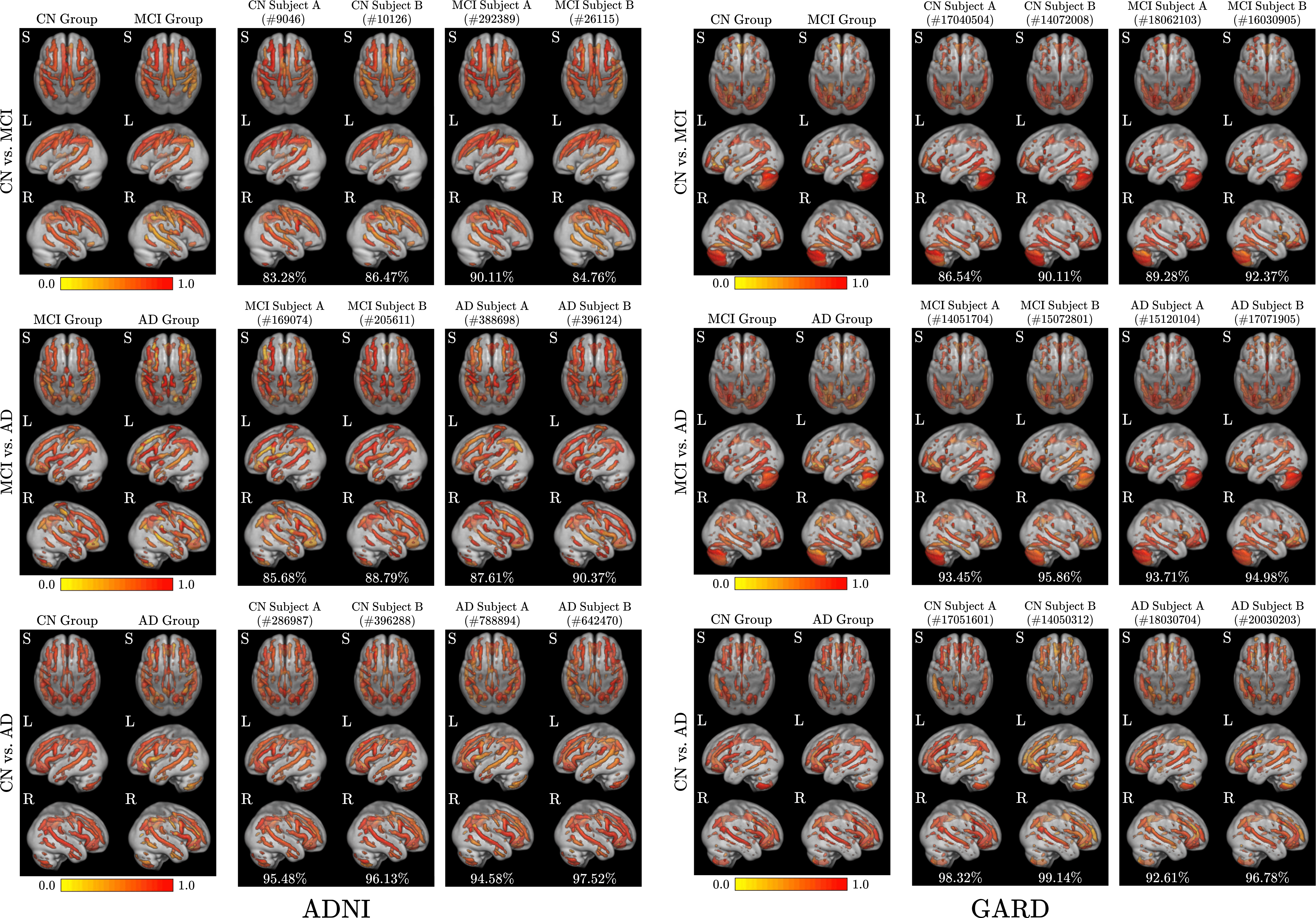
By exploiting the simplified function in Supplementary H, we analyzed the input-dependent representation of (termed AD-relatedness index) that revealed the contribution of each ROI for patient-specific prediction. We used the counterfactual-guided attention map as the region-wise AD-related importance to support the LiCoL decision in any classification scenario. In Fig. 5, we illustrate the region-wise AD-relatedness indices over the group and individual patients in each scenario on ADNI and GARD datasets. For the group-wise investigation (first column in the ADNI and GARD results), we averaged the AD-relatedness indices for all test samples corresponding to the respective clinical stage. Among all scenarios related to the group-wise investigation, we observed that the majority of AD-effect ROIs for CN AD were closely related to the AD prediction (i.e., most red-colored regions). In this scenario, as the morphological difference w.r.t brain atrophies were relatively immense, our LiCoL attended to the most ROIs with prominent GM density changes. Meanwhile, the AD-relatedness index for individual patients (second and third columns in the ADNI and GARD results) was randomly visualized among the arbitrary longitudinal subjects that were accurately classified with high confidence (i.e., accuracy). It was intriguing that each patient revealed a varying AD-related index despite being guided by a coherent AD-effect ROIs . This showed that our LiCoL considered the regional differences in GM density between clinical groups and reflected the individual discriminative characteristics regarding the patient’s status.
Overall, the ROIs of L/R.HIP, L/R.STG, L/R.IFGoperc, and L.PreCG exhibited especially high AD-relatedness indices among AD-effect ROIs in all scenarios. Particularly, the HIP is one of the prominent regions that shows atrophy in AD [51] and is treated as an index of AD neuropathology [52]. This region is further related to the MCI [53] or the early marker [54]. The temporal region composed of STG is known as a region where structural variations occur in the AD-manifested brain [55]. In CN MCI and CN AD scenarios, R.INS and L/R.PCUN did not exhibit as essential ROIs for CN prediction, whereas those ROIs appeared as crucial markers when used to diagnose MCI or AD patients [51, 34]. Notably, L.SMA was an ROI that markedly contributed to diagnosing MCI, and R.IPG was found to have a significant ROI with a high AD-relatedness index in AD. Additionally, the regions of L/R.SFG and L/R.MFG, located in the frontal area, are also captured in all scenarios, which is associated with AD [55]. Based on in-depth analyses via LiCoL’s transparency, we clinically validated that the DL model (i.e., CMG) well-generated the target properties of which regions in the brain to change the classifier’s prediction to the target class as the brain disease progressed. Thereby, AD-relatedness indices could provide neuroscientific insights for disease stratification in patient groups and understanding of individuals’ symptoms, facilitating the direction of more specified diagnostic criteria for personalized inspection.
| Data | Age | MCI | AD | w/ cGM | (Ours) | ||||
|---|---|---|---|---|---|---|---|---|---|
| (years) | Precision | Recall | Precision | Recall | Precision | Recall | |||
| ADNI | 206 | 65 | 0.6897 | 0.8995 | 0.7871 | 0.9144 | 0.8313 | 0.9331 | |
| 359 | 174 | 0.8201 | 0.9067 | 0.8641 | 0.9356 | 0.8951 | 0.9415 | ||
| 149 | 101 | 0.7273 | 0.9331 | 0.8318 | 0.9428 | 0.8491 | 0.9628 | ||
| GARD | 130 | 19 | 0.6338 | 0.9339 | 0.7452 | 0.9773 | 0.7780 | 0.9840 | |
| 181 | 53 | 0.7016 | 0.9211 | 0.7838 | 0.9276 | 0.8093 | 0.9777 | ||
| 50 | 34 | 0.5742 | 0.8942 | 0.7661 | 0.8997 | 0.7957 | 0.9146 | ||
3.8 Counterfactual images for spurious correlations
We further explored whether issues encountered in the medical field could be overcome using cGM augmentation. Indeed, accurate prevalence estimates of dementia by age, or other demographic information for different levels of severity could support effective medical treatment. Particularly, age constitutes the greatest of the various risk factors w.r.t AD manifestation, with the percentage of the population who have AD increasing dramatically with age. However, although 3% of people aged 65 74, 17% of people aged 75 84, and 32% of people aged 85 or older have been diagnosed as AD patients [56], it is important to note that AD is not a normal part of aging [57], and older age alone is not considered a sufficient factor to cause AD. Various medical studies [58, 59] call this phenomenon spurious correlation, which occurs when two factors appear to be correlated to each other, but in fact are not [60]. Furthermore, few AD cases are identified when the patient’s age is younger than 65 years, and further data on the prevalence of brain disease are scarce. Hence, samples of a specific age or clinical stage are lacking, which leads to an undesirable bias. We thus exploited the cGMs as augmented samples to alleviate these practical issues. For this purpose, we used the set of and as the classifier’s input (use our LiCoL) to demonstrate the fidelity of cGM augmentation by showing that the performance shifts, which depend on whether augmented data are included in the training.
As reported in Table IV, the precision of the trained LiCoL that used was found to be relatively lower in young AD (i.e., aged 60 70) on ADNI as well as elderly MCI (i.e., aged 80 90) on GARD. Furthermore, unlike in the ADNI, a lack of samples appeared in the 80 90 age range in GARD, and this age range exhibited the lowest precision. In this light, we can assume that precision degradation was derived due to the undesirable spurious correlation. However, when statistical ROIs were constructed along with cGM (i.e., w/ cGM), the performance with augmentation was noticeably improved across all age ranges. Particularly, it should be noted that the precision for the aged 80 90 on GARD dramatically increased by +19.19%. Through these results, we argued that the auxiliary cGMs of a patient at different clinical stages provided informative features, so that LiCoL could learn how to correctly distinguish the discriminative characteristics of each clinical stage, depending on the age range. Thus, we suggest distilling cGMs can be beneficial for mitigating the data-hungry problem in practical settings and promising alternatives for solving spurious correlations.
4 Discussion
The goal of GM density manipulation in this study is to normalize the individual brain image so that it aligns to a consistent anatomical space to account for personal variability. From this perspective, GM density maps might induce the disappearance of individual-specific shape information and minor structural distortions due to mapping into the shared template during the manipulation. However, contrary to these concerns, the variations in density values across the GM density maps after registration still represent crucial information. GM density maps take into account the fact that the size and shape of brains can vary considerably among individuals during the registration process; hence GM density values within these maps present GM volume so that it enables us to facilitate meaningful comparisons by focusing on the quantity of GM density. Furthermore, these maps are sensitive to subtle variations in the GM volume or concentration, which may occur in the early stages of AD manifestation, even before morphological changes are visible on linear-registered MRI scans. Thanks to such advantages, it can better depict brain atrophies, a hallmark of Alzheimer’s or other neurodegenerative diseases, making it widely used in medical image analysis as one of the quantitative features [34, 61, 62]. Nonetheless, exploiting the entire GM density maps alone might be inadequate for AD classification as it is hard to capture the subtle structural variations because of the aligning process. To overcome this drawback, we further utilized the ROI strategy to focus on specific regions where the GM density differences occur depending on the disease progression. In particular, since our AD-effect ROIs are only constructed via GM density values in highlighted regions that are quite sensitive to the variability of AD influence and highly related to AD manifestation, it is possible to boost the effectiveness of the ROI-based classification. To further verify the applicability of such in-depth analysis, an extensive evaluation was performed by utilizing other promising counterfactual-based approaches, as reported in Supplementary K.
Our predictive evaluation showed that LiCoL, despite being a linear classifier, outperformed all the comparative ML-based models considered in our study with substantial margins and was comparable to DL-based models. Under the linear property, We have further demonstrated that our LiCoL possesses a monotonicity similar to ML-based models, which are prone to comprehend the internal working. In particular, through the AD-relatedness index induced by the LiCoL’s inherent transparency, we could observe that each patient and group had a different contribution within ROIs, depending on the severity of morphological variations. By virtue of the LiCoL’s superiority, we thus claim that our method could be a stepping stone toward a comprehensible explanation of the deep models’ decisions and for predicting and analyzing neurodegenerative disease by leveraging quantitative figures.
5 Conclusion
In this work, we proposed a novel framework to analyze the counterfactual-induced visual explainability by transforming them into a GM density as a quantitative feature representation. Quantitative feature-based analysis using AD-effect ROIs helped conduct accurate numerical measurements based on the volumetric density changes in the brain caused by AD progression. Additionally, we designed a LiCoL, a simple shallow linear classifier, to boost the effectiveness of AD-effect ROIs while providing outstanding performance and the model’s interpretability. Under LiCoL’s transparency, we further produced an AD-relatedness index that can be identified to intuitively understand the AD-related landmarks for an individual subject and groups.
We have viewed that utilizing visual explanation manipulated to quantitative figures is beneficial in yielding neuroscientific insights from a clinical aspect. However, there is still marginal room for improvement. Indeed, counterfactual reasoning regarding causality has to consider various confounders such as age, gender, or genetic factors, and the classification performance over multi-class scenarios must also be enhanced to provide more reliable interpretability. In this context, the future direction of this research would like to develop a model that adequately incorporates such demographic factors based on mutual relationships and derives outstanding performance in the multi-class scenarios while accounting for the nuanced differences among several disease stages via quantitative interpretation accordingly.
Acknowledgement
This work was supported by the Institute of Information & communications Technology Planning & Evaluation (IITP) grant funded by the Korea government (MSIT) No. 2022-0-00959 ((Part 2) Few-Shot Learning of Causal Inference in Vision and Language for Decision Making) and No. 2019-0-00079 (Department of Artificial Intelligence (Korea University)). This study was further supported by KBRI basic research program through Korea Brain Research Institute funded by the Ministry of Science and ICT (22-BR-03-05).
References
- [1] Alzheimer’s Association, “2019 Alzheimer’s disease facts and figures,” Alzheimer’s & Dementia, vol. 15, no. 3, pp. 321–387, 2019.
- [2] M. W. Weiner, D. P. Veitch, P. S. Aisen, L. A. Beckett, N. J. Cairns, R. C. Green, D. Harvey, C. R. Jack, W. Jagust, E. Liu et al., “The Alzheimer’s disease neuroimaging initiative: A review of papers published since its inception,” Alzheimer’s & Dementia, vol. 9, no. 5, pp. e111–e194, 2013.
- [3] J. L. Cummings, R. Doody, and C. Clark, “Disease-modifying therapies for Alzheimer disease: Challenges to early intervention,” Neurology, vol. 69, no. 16, pp. 1622–1634, 2007.
- [4] R. C. Petersen, R. O. Roberts, D. S. Knopman, B. F. Boeve, Y. E. Geda, R. J. Ivnik, G. E. Smith, and C. R. Jack, “Mild cognitive impairment: Ten years later,” Archives of Neurology, vol. 66, no. 12, pp. 1447–1455, 2009.
- [5] J. A. Schneider, Z. Arvanitakis, S. E. Leurgans, and D. A. Bennett, “The neuropathology of probable Alzheimer disease and mild cognitive impairment,” Annals of Neurology: Official Journal of the American Neurological Association and the Child Neurology Society, vol. 66, no. 2, pp. 200–208, 2009.
- [6] H. J. Aerts, E. R. Velazquez, R. T. Leijenaar, C. Parmar, P. Grossmann, S. Carvalho, J. Bussink, R. Monshouwer, B. Haibe-Kains, D. Rietveld et al., “Decoding tumour phenotype by noninvasive imaging using a quantitative radiomics approach,” Nature Communications, vol. 5, no. 1, pp. 1–9, 2014.
- [7] K.-H. Yu, C. Zhang, G. J. Berry, R. B. Altman, C. Ré, D. L. Rubin, and M. Snyder, “Predicting non-small cell lung cancer prognosis by fully automated microscopic pathology image features,” Nature Communications, vol. 7, no. 1, pp. 1–10, 2016.
- [8] R. J. Gillies, P. E. Kinahan, and H. Hricak, “Radiomics: Images are more than pictures, they are data,” Radiology, vol. 278, no. 2, pp. 563–577, 2016.
- [9] M. López, J. Ramírez, J. Górriz, I. Álvarez, D. Salas-Gonzalez, F. Segovia, and R. Chaves, “SVM-based CAD system for early detection of the Alzheimer’s disease using kernel PCA and LDA,” Neuroscience Letters, vol. 464, no. 3, pp. 233–238, 2009.
- [10] H. Zhou, J. Jiang, J. Lu, M. Wang, H. Zhang, C. Zuo, and Alzheimer’s Disease Neuroimaging Initiative and others, “Dual-model radiomic biomarkers predict development of mild cognitive impairment progression to Alzheimer’s disease,” Frontiers in Neuroscience, vol. 12, p. 1045, 2019.
- [11] S. Lee, H. Lee, and K. W. Kim, “Magnetic resonance imaging texture predicts progression to dementia due to Alzheimer disease earlier than hippocampal volume,” Journal of Psychiatry and Neuroscience, vol. 45, no. 1, pp. 7–14, 2020.
- [12] H. Ij, “Statistics versus machine learning,” Nature Methods, vol. 15, no. 4, p. 233, 2018.
- [13] Z. Li, H. Duan, K. Zhao, and Y. Ding, “Stability of MRI radiomics features of hippocampus: An integrated analysis of test-retest and inter-observer variability,” IEEE Access, vol. 7, pp. 97 106–97 116, 2019.
- [14] K. Zhao, Y. Ding, Y. Han, Y. Fan, A. F. Alexander-Bloch, T. Han, D. Jin, B. Liu, J. Lu, C. Song et al., “Independent and reproducible hippocampal radiomic biomarkers for multisite Alzheimer’s disease: Diagnosis, longitudinal progress and biological basis,” Science Bulletin, vol. 65, no. 13, pp. 1103–1113, 2020.
- [15] Y. LeCun, Y. Bengio, and G. Hinton, “Deep learning,” Nature, vol. 521, no. 7553, pp. 436–444, 2015.
- [16] J. Venugopalan, L. Tong, H. R. Hassanzadeh, and M. D. Wang, “Multimodal deep learning models for early detection of Alzheimer’s disease stage,” Scientific Reports, vol. 11, no. 1, pp. 1–13, 2021.
- [17] X. Zhang, L. Han, W. Zhu, L. Sun, and D. Zhang, “An explainable 3D residual self-attention deep neural network for joint atrophy localization and Alzheimer’s disease diagnosis using structural MRI,” IEEE Journal of Biomedical and Health Informatics, 2021.
- [18] Z. Yang, I. M. Nasrallah, H. Shou, J. Wen, J. Doshi, M. Habes, G. Erus, A. Abdulkadir, S. M. Resnick, M. S. Albert et al., “A deep learning framework identifies dimensional representations of Alzheimer’s disease from brain structure,” Nature Communications, vol. 12, no. 1, pp. 1–15, 2021.
- [19] A. Adadi and M. Berrada, “Peeking inside the black-box: A survey on explainable artificial intelligence (XAI),” IEEE Access, vol. 6, pp. 52 138–52 160, 2018.
- [20] A. B. Arrieta, N. Díaz-Rodríguez, J. Del Ser, A. Bennetot, S. Tabik, A. Barbado, S. García, S. Gil-López, D. Molina, R. Benjamins et al., “Explainable artificial intelligence (XAI): Concepts, taxonomies, opportunities and challenges toward responsible AI,” Information Fusion, vol. 58, pp. 82–115, 2020.
- [21] M. Sundararajan, A. Taly, and Q. Yan, “Axiomatic attribution for deep networks,” in 34th International Conference on Machine Learning, 2017, pp. 3319–3328.
- [22] R. R. Selvaraju, M. Cogswell, A. Das, R. Vedantam, D. Parikh, and D. Batra, “Grad-CAM: Visual explanations from deep networks via gradient-based localization,” in IEEE International Conference on Computer Vision, 2017, pp. 618–626.
- [23] Y. Wang, H. Su, B. Zhang, and X. Hu, “Learning reliable visual saliency for model explanations,” IEEE Transactions on Multimedia, vol. 22, no. 7, pp. 1796–1807, 2019.
- [24] R. M. Byrne, “Counterfactuals in explainable artificial intelligence (XAI): Evidence from human reasoning.” in International Joint Conference on Artificial Intelligence, 2019, pp. 6276–6282.
- [25] Y. Goyal, Z. Wu, J. Ernst, D. Batra, D. Parikh, and S. Lee, “Counterfactual visual explanations,” in 36th International Conference on Machine Learning, 2019, pp. 2376–2384.
- [26] I. Goodfellow, “NIPS 2016 tutorial: Generative adversarial networks,” arXiv preprint arXiv:1701.00160, 2016.
- [27] M. Mirza and S. Osindero, “Conditional generative adversarial nets,” arXiv preprint arXiv:1411.1784, 2014.
- [28] S. Dash, V. Balasubramanian, and A. Sharma, “Evaluating and mitigating bias in image classifiers: A causal perspective using counterfactuals,” in Winter Conference on Applications of Computer Vision, January 2022, pp. 915–924.
- [29] K. Oh, J. S. Yoon, and H.-I. Suk, “Learn-explain-reinforce: Counterfactual reasoning and its guidance to reinforce an Alzheimer’s disease diagnosis model,” IEEE Transactions on Pattern Analysis and Machine Intelligence, vol. 45, no. 4, pp. 4843–4857, 2022.
- [30] T. Xia, A. Chartsias, C. Wang, S. A. Tsaftaris, A. D. N. Initiative et al., “Learning to synthesise the ageing brain without longitudinal data,” Medical Image Analysis, vol. 73, p. 102169, 2021.
- [31] D. W. Kim, H. Y. Jang, K. W. Kim, Y. Shin, and S. H. Park, “Design characteristics of studies reporting the performance of artificial intelligence algorithms for diagnostic analysis of medical images: Results from recently published papers,” Korean Journal of Radiology, vol. 20, no. 3, pp. 405–410, 2019.
- [32] X. Zhang, E. C. Mormino, N. Sun, R. A. Sperling, M. R. Sabuncu, B. T. Yeo, and A. D. N. Initiative, “Bayesian model reveals latent atrophy factors with dissociable cognitive trajectories in Alzheimer’s disease,” Proceedings of the National Academy of Sciences, vol. 113, no. 42, pp. E6535–E6544, 2016.
- [33] Y. Hirata, H. Matsuda, K. Nemoto, T. Ohnishi, K. Hirao, F. Yamashita, T. Asada, S. Iwabuchi, and H. Samejima, “Voxel-based morphometry to discriminate early Alzheimer’s disease from controls,” Neuroscience Letters, vol. 382, no. 3, pp. 269–274, 2005.
- [34] G. Karas, P. Scheltens, S. A. Rombouts, P. J. Visser, R. A. van Schijndel, N. C. Fox, and F. Barkhof, “Global and local gray matter loss in mild cognitive impairment and Alzheimer’s disease,” NeuroImage, vol. 23, no. 2, pp. 708–716, 2004.
- [35] C. Davatzikos, F. Xu, Y. An, Y. Fan, and S. M. Resnick, “Longitudinal progression of Alzheimer’s-like patterns of atrophy in normal older adults: The SPARE-AD index,” Brain, vol. 132, no. 8, pp. 2026–2035, 2009.
- [36] S. G. Mueller, M. W. Weiner, L. J. Thal, R. C. Petersen, C. Jack, W. Jagust, J. Q. Trojanowski, A. W. Toga, and L. Beckett, “The Alzheimer’s disease neuroimaging initiative,” Neuroimaging Clinics of North America, vol. 15, no. 4, pp. 869 – 877, 2005.
- [37] K. Y. Choi, J. J. Lee, T. I. Gunasekaran, S. Kang, W. Lee, J. Jeong, H. J. Lim, X. Zhang, C. Zhu, S.-Y. Won et al., “APOE promoter polymorphism-219T/G is an effect modifier of the influence of APOE 4 on Alzheimer’s disease risk in a multiracial sample,” Journal of Clinical Medicine, vol. 8, no. 8, p. 1236, 2019.
- [38] O. Ronneberger, P. Fischer, and T. Brox, “U-Net: Convolutional networks for biomedical image segmentation,” in International Conference on Medical Image Computing and Computer-Assisted Intervention, 2015, pp. 234–241.
- [39] X. Mao, Q. Li, H. Xie, R. Y. Lau, Z. Wang, and S. Paul Smolley, “Least squares generative adversarial networks,” in Proceedings of the IEEE International Conference on Computer Vision, 2017, pp. 2794–2802.
- [40] J.-Y. Zhu, T. Park, P. Isola, and A. A. Efros, “Unpaired image-to-image translation using cycle-consistent adversarial networks,” in IEEE International Conference on Computer Vision, 2017, pp. 2223–2232.
- [41] Y. Zhang, M. Brady, and S. Smith, “Segmentation of brain MR images through a hidden Markov random field model and the expectation-maximization algorithm,” IEEE Transactions on Medical Imaging, vol. 20, no. 1, pp. 45–57, 2001.
- [42] E. T. Rolls, C.-C. Huang, C.-P. Lin, J. Feng, and M. Joliot, “Automated anatomical labelling atlas 3,” NeuroImage, vol. 206, p. 116189, 2020.
- [43] A. Vaswani, N. Shazeer, N. Parmar, J. Uszkoreit, L. Jones, A. N. Gomez, L. u. Kaiser, and I. Polosukhin, “Attention is all you need,” in Advances in Neural Information Processing Systems, vol. 30, 2017, pp. 6000–6010.
- [44] J. Davis and M. Goadrich, “The relationship between precision-recall and ROC curves,” in Proceedings of the 23rd International Conference on Machine Learning, 2006, pp. 233–240.
- [45] S. L. Risacher, A. J. Saykin, J. D. Wes, L. Shen, H. A. Firpi, and B. C. McDonald, “Baseline MRI predictors of conversion from MCI to probable AD in the ADNI cohort,” Current Alzheimer Research, vol. 6, no. 4, pp. 347–361, 2009.
- [46] C. Jack, M. Shiung, J. Gunter, P. O’brien, S. Weigand, D. S. Knopman, B. F. Boeve, R. Ivnik, G. Smith, R. Cha et al., “Comparison of different MRI brain atrophy rate measures with clinical disease progression in AD,” Neurology, vol. 62, no. 4, pp. 591–600, 2004.
- [47] K. He, X. Zhang, S. Ren, and J. Sun, “Deep residual learning for image recognition,” in Proceedings of the IEEE Conference on Computer Vision and Pattern Recognition, 2016, pp. 770–778.
- [48] A. Dosovitskiy, L. Beyer, A. Kolesnikov, D. Weissenborn, X. Zhai, T. Unterthiner, M. Dehghani, M. Minderer, G. Heigold, S. Gelly et al., “An image is worth 16x16 words: Transformers for image recognition at scale,” in International Conference on Learning Representations, 2021.
- [49] J. Jang and D. Hwang, “M3T: three-dimensional medical image classifier using multi-plane and multi-slice Transformer,” in Proceedings of the IEEE/CVF Conference on Computer Vision and Pattern Recognition, 2022, pp. 20 718–20 729.
- [50] J. Zhang, L. Zhou, L. Wang, M. Liu, and D. Shen, “Diffusion kernel attention network for brain disorder classification,” IEEE Transactions on Medical Imaging, vol. 41, no. 10, pp. 2814–2827, 2022.
- [51] A. L. Foundas, C. M. Leonard, S. M. Mahoney, O. F. Agee, and K. M. Heilman, “Atrophy of the hippocampus, parietal cortex, and insula in Alzheimer’s disease: A volumetric magnetic resonance imaging study.” Neuropsychiatry, Neuropsychology, & Behavioral Neurology, 1997.
- [52] K. Gosche, J. Mortimer, C. Smith, W. Markesbery, and D. Snowdon, “Hippocampal volume as an index of Alzheimer neuropathology: Findings from the nun study,” Neurology, vol. 58, no. 10, pp. 1476–1482, 2002.
- [53] R. S. Desikan, H. J. Cabral, C. P. Hess, W. P. Dillon, C. M. Glastonbury, M. W. Weiner, N. J. Schmansky, D. N. Greve, D. H. Salat, R. L. Buckner et al., “Automated MRI measures identify individuals with mild cognitive impairment and Alzheimer’s disease,” Brain, vol. 132, no. 8, pp. 2048–2057, 2009.
- [54] M. De Leon, A. George, L. Stylopoulos, G. Smith, and D. Miller, “Early marker for Alzheimer’s disease: The atrophic hippocampus,” The Lancet, vol. 334, no. 8664, pp. 672–673, 1989.
- [55] C. Davies, D. Mann, P. Sumpter, and P. Yates, “A quantitative morphometric analysis of the neuronal and synaptic content of the frontal and temporal cortex in patients with Alzheimer’s disease,” Journal of the Neurological Sciences, vol. 78, no. 2, pp. 151–164, 1987.
- [56] L. E. Hebert, J. Weuve, P. A. Scherr, and D. A. Evans, “Alzheimer disease in the United States (2010–2050) estimated using the 2010 census,” Neurology, vol. 80, no. 19, pp. 1778–1783, 2013.
- [57] P. T. Nelson, E. Head, F. A. Schmitt, P. R. Davis, J. H. Neltner, G. A. Jicha, E. L. Abner, C. D. Smith, L. J. Van Eldik, R. J. Kryscio et al., “Alzheimer’s disease is not “brain aging”: Neuropathological, genetic, and epidemiological human studies,” Acta Neuropathologica, vol. 121, no. 5, pp. 571–587, 2011.
- [58] A. J. DeGrave, J. D. Janizek, and S.-I. Lee, “AI for radiographic COVID-19 detection selects shortcuts over signal,” Nature Machine Intelligence, vol. 3, no. 7, pp. 610–619, 2021.
- [59] U. Mahmood, R. Shrestha, D. D. Bates, L. Mannelli, G. Corrias, Y. E. Erdi, and C. Kanan, “Detecting spurious correlations with sanity tests for artificial intelligence guided radiology systems,” Frontiers in Digital Health, vol. 3, p. 671015, 2021.
- [60] H. A. Simon, “Spurious correlation: A causal interpretation,” Journal of the American Statistical Association, vol. 49, no. 267, pp. 467–479, 1954.
- [61] G. Karas, P. Scheltens, S. Rombouts, R. Van Schijndel, M. Klein, B. Jones, W. Van Der Flier, H. Vrenken, and F. Barkhof, “Precuneus atrophy in early-onset alzheimer’s disease: a morphometric structural mri study,” Neuroradiology, vol. 49, pp. 967–976, 2007.
- [62] L. G. Apostolova, C. A. Steiner, G. G. Akopyan, R. A. Dutton, K. M. Hayashi, A. W. Toga, J. L. Cummings, and P. M. Thompson, “Three-dimensional gray matter atrophy mapping in mild cognitive impairment and mild alzheimer disease,” Archives of neurology, vol. 64, no. 10, pp. 1489–1495, 2007.
![[Uncaptioned image]](/html/2310.03457/assets/authors/oh.jpg) |
Kwanseok Oh received the B.S. degree in Electronic Control and Engineering from Hanbat National University, Daejeon, South Korea, in 2020. He is currently pursuing a Ph.D. degree with the Department of Artificial Intelligence, Korea University, Seoul, South Korea. His current research interests include explainable AI, computer vision, and machine/deep learning. |
![[Uncaptioned image]](/html/2310.03457/assets/authors/heo.jpg) |
Da-Woon Heo received the M.S. degree in Brain and Cognitive Engineering from Korea University, Seoul, South Korea, in 2018. She is currently pursuing a Ph.D. degree with the Department of Artificial Intelligence, Korea University, Seoul, South Korea. Her current research interests include machine/deep learning, medical AI, and neuroscience. |
![[Uncaptioned image]](/html/2310.03457/assets/authors/wisnu.jpg) |
Ahmad Wisnu Mulyadi received the B.S. degree in Computer Science Education from the Indonesia University of Education, Bandung, Indonesia, in 2010. He is currently pursuing a Ph.D. degree with the Department of Brain and Cognitive Engineering, Korea University, Seoul, South Korea. His current research interests include machine/deep learning in healthcare, biomedical image analysis, and graph representation learning. |
![[Uncaptioned image]](/html/2310.03457/assets/authors/jung.jpg) |
Wonsik Jung received the B.S. degree in Bio Medical Engineering from Konyang University, Daejeon, South Korea, in 2018. He is currently pursuing a Ph.D. degree with the Department of Brain and Cognitive Engineering, Korea University, Seoul, South Korea. His current research interests include computer vision, time-series modeling, and representation learning. |
![[Uncaptioned image]](/html/2310.03457/assets/authors/kang.jpg) |
Eunsong Kang received the B.S. degree in Psychology from Korea University, Seoul, South Korea, in 2017. She is currently pursuing a Ph.D. degree with the Department of Brain and Cognitive Engineering, Korea University, Seoul, South Korea. Her current research interests include explainable AI, time-series modeling, and medical image analysis. |
![[Uncaptioned image]](/html/2310.03457/assets/authors/lee2.png) |
Kun Ho Lee received the B.S. degree from the Department of Genetic Engineering, Korea University, Seoul, Republic of Korea, in 1989, and the M.S. and Ph.D. degrees from the Department of Molecular Biology, Seoul National University, Seoul, in 1994 and 1998, respectively. He is currently an Associate Professor with the Department of Biomedical Science, Chosun University, Gwangju, Republic of Korea. He also works with the National Research Center for Dementia, Chosun University. His current research interests include brain image analysis and the development of prediction model for neurodegenerative diseases based on MRI and genetic variants. |
![[Uncaptioned image]](/html/2310.03457/assets/authors/prof_suk.jpeg) |
Heung-Il Suk received the B.S. and M.S. degrees in Computer Engineering from Pukyong National University, Busan, Korea, in 2004 and 2007, respectively, and the Ph.D. degree in Computer Science and Engineering from Korea University, Seoul, South Korea, in 2012. From 2012 to 2014, he was a Post-Doctoral Research Associate with the University of North Carolina at Chapel Hill, Chapel Hill, NC, USA. He is currently an Associate Professor at the Department of Artificial Intelligence and the Department of Brain and Cognitive Engineering, Korea University. He was awarded a Kakao Faculty Fellowship from Kakao and a Young Researcher Award from the Korean Society for Human Brain Mapping (KHBM) in 2018 and 2019, respectively. His research interests include machine/deep learning, explainable AI, biomedical data analysis, and brain-computer interface. Dr. Suk serves as an Editorial Board Member for Electronics, Frontiers in Neuroscience, Frontiers in Radiology, International Journal of Imaging Systems and Technology (IJIST), Clinical and Molecular Hepatology, and a Program Committee or a Reviewer for international conferences, including NeurIPS, ICML, ICLR, AAAI, IJCAI, CVPR, MICCAI, IPMI, MIDL, etc. |