Variational Inference for GARCH-family Models

Abstract

The Bayesian estimation of GARCH-family models has been typically addressed through Monte Carlo sampling. Variational Inference is gaining popularity and attention as a robust approach for Bayesian inference in complex machine learning models; however, its adoption in econometrics and finance is limited. This paper discusses the extent to which Variational Inference constitutes a reliable and feasible alternative to Monte Carlo sampling for Bayesian inference in GARCH-like models. Through a large-scale experiment involving the constituents of the S&P 500 index, several Variational Inference optimizers, a variety of volatility models, and a case study, we show that Variational Inference is an attractive, remarkably well-calibrated, and competitive method for Bayesian learning.

I Introduction

The classical estimation procedures for GARCH-family modes are the frequentist maximum likelihood, quasi maximum likelihood, and the generalized method of moments approaches [6]. Recently, there has been a growing interest in using Bayesian estimation techniques, as they offer several advantages over the traditional approaches [7]. For instance, in the frequentist approach, models are compared with no other means that their likelihood, whereas Bayes factors and marginal likelihood allow comparisons of non-nested models. Bayesian estimation provides reliable results in finite samples, and, e.g., can uncover the full value-at-risk density. Maximum likelihood estimators present some limitations when the errors are heavy-tailed and may not be asymptotically Gaussian [11], and positivity of the conditional variance and stationarity requirements can lead to complex non-linear inequalities, making constrained optimization cumbersome. For the Bayesian estimation of GARCH-family models, Monte Carlo (MC) sampling is the predominant approach [e.g., 11, 1, 28]. Indeed the recursive nature of the conditional variance makes the joint posterior of unknown parametric form, and the choice of the sampling algorithm is crucial. The Griddy-Gibbs sampler has extensively been used in this context [e.g., 5, 3], along with importance sampling [e.g., 9, 13], and the Metropolis-Hastings (MH) [18, 8]. Different extensions of the MH algorithm have been proposed [e.g., 19], along with the use of alternative methods [e.g., 2]. For a broader overview, see, e.g., the surveys [7, 28], or the textbook [1].

The ability of Bayesian methods to address uncertainty via posterior distribution gained much attention in Machine Learning (ML). In the last decade, sophisticated Bayesian methods have been advanced for training high-dimensional ML models, and the theory of Bayesian neural networks has been extensively developed [see, e.g., 15, for a review]. Under the complexity of typical ML models, sampling methods do not scale up in high dimensions and difficult to apply. Variational Inference (VI) stands as a successful and feasible alternative, widely exploited in ML applications [12, 25, 14]. VI reduces the typical Bayesian integration problem to a simpler optimization problem aimed at finding the “best” approximation of the true posterior distribution in the sense described in Sec. II-B. Despite its consolidated use in ML, VI has not received much attention in econometrics and finance as a feasible Bayesian alternative to MC sampling.

In particular, the use of VI as a tool for the Bayesian estimation of GARCH-family models remains unaddressed. Though VI has been used in volatility forecasting with ML models [22, 21], there have been few self-contained VI applications concerning GARCH models [17, 16, 27]. This paper fills the this gap and addresses the feasibility and appropriateness of VI as an alternative to MC sampling and maximum likelihood estimation by conducting extensive experiments on the constituents of the S&P500 index. We show how Gaussian VI can be implemented and applied at a large scale as an unconstrained optimization problem through appropriate parameter transforms. We validate the results over several in-sample and out-of-sample performance metrics. Along with a focused study on the Microsoft Inc. stock data, with different optimization algorithms, we show VI is an effective, robust, and competitive approach for the Bayesian estimation of various GARCH-family models.

II Methods

II-A GARCH models

A major task of financial econometrics is modeling volatility in asset returns. Volatility is considered a measure of risk for which investors demand a premium for investing in risky assets. Empirical observations of financial returns reveal some stylized facts. Whereas returns are nearly uncorrelated, they contain higher-order dependences. The correlation of absolute and squared returns is positive and persistent. Autocorrelated daily volatility thus appears to be predictable, and Autoregressive Conditional Heteroskedasticity (ARCH) models provide the basis for the most popular parameterizations of this dependence.

Let $\varepsilon_{t}$ be a random variable that has mean and variance conditionally on the information set $\mathcal{F}_{t-1}$ ($\sigma$-algebra generated by $\varepsilon_{t-j},j\geq 1$). For the ARCH model, $\mathbb{E}\left(\varepsilon_{t}|\mathcal{F}_{t-1}\right)=0$ and the conditional variance $h_{t}=\mathbb{E}\left(\varepsilon^{2}_{t}|\mathcal{F}_{t}\right)$ is a parametric function on $\mathcal{F}_{t-1}$ [26]. The sequence $\{\varepsilon_{t}\}$ may be observed or be an error innovation sequence of an econometric model: $\varepsilon_{t}=r_{t}-\mu_{t}\left(r_{t}\right)$ with $r_{t}$ and observable random variable (e.g., a daily return) and $\mu_{t}\left(r_{t}\right)$ the conditional expectation of $r_{t}$ given $\mathcal{F}_{t-1}$. The parametric form of the ARCH model reads:

$$r_{t} =\mu+\varepsilon_{t},$$

$$\varepsilon_{t} =h^{1/2}_{t}z_{t}\text{,}\quad z_{t}\sim\text{{iid }}\mathcal{N}\left(0,1\right),$$

$$h_{t} =\omega+\alpha_{1}\varepsilon^{2}_{t-1},$$

with $t=1,\dots,T$ and, to ensure $h_{t}>0$ and identification, $\omega>0$, $0<\alpha_{1}<1$. We shall assume $\mu\equiv 0$. $h_{t}$ is the conditional and time-dependent volatility of $\varepsilon_{t}$. The way $\varepsilon_{t}$ is defined guarantees white noise properties, since $z_{t}$ is a sequence of iid variables. Normality is a typical assumption for the iid sequence $\{z_{t}\}$, but leptokurtic alternatives are also used. The iid assumption guarantees the white noise property of $\{\varepsilon_{t}\}$. In the ARCH equation defining the parametric form for the conditional variance, the linear function of the squared innovation at $t-1$ can be generalized to a higher-order ARCH$(q)$:

$$h_{t}=\omega+\sum_{j=1}^{q}\alpha_{j}\varepsilon^{2}_{t-j},$$

where $\omega>0,\,\alpha_{j}\geq 0$, with at least an $\alpha_{j}>0$. Note that the volatility, the object of modeling, is not observed: using $\varepsilon^{2}_{t}$ is an immediate solution, but alternatives exist if, e.g., the data is available at intraday frequencies.

For the ARCH family, the decay rate in the autocorrelation of $\varepsilon_{t}^{2}$ is too rapid compared to the observed time series: the so-called Generalized ARCH (GARCH) is a predominant alternative. In a GARCH$(p,q)$ model, the conditional variance is not only a function of the lagged innovations but also of its lags:

$$h_{t}=\omega+\sum_{j=1}^{q}\alpha_{j}\varepsilon^{2}_{t-j}+\sum_{j=1}^{p}\beta_{j}h_{t-j}.$$

The overwhelming model has been the GARCH$(1,1)$. Sufficient conditions for the positivity of conditional variances are $\omega>0$, $\alpha_{j}\geq 0$, $j=1,\dots,q$ and $\beta_{j}\geq 0$, $j=1,\dots,p$. Identifiability requires at least one $\beta_{j}>0$ and one $\alpha_{j}>0$, and for stationarity $\sum\alpha_{j}+\sum\beta_{j}<1$.

GARCH models have been extended and generalized in many different directions. Among these, the empirical evidence of asymmetry in volatility clustering motivates the GJR-GARCH [10] model, which assumes the response of the variance to a shock not to be independent of its sign:

$$h_{t}=\omega+\sum_{j=1}^{q}\alpha_{j}+\sum_{j=1}^{o}\gamma_{j}I\left(\varepsilon_{t-j}>0\right)\varepsilon^{2}_{t-j}+\sum_{j=1}^{p}\beta_{j}h_{t-j},$$

with $I\left(\cdot\right)$ an indicator function, defines the GJR-GARCH$(p,o,q)$ (with $o=0$ we simply write GJR-GARCH$(p,q)$). It must hold $\omega>0$, $\alpha_{j}\geq 0$, $\beta_{j}\geq 0$, $\gamma_{j}\geq 0$, $\sum\alpha_{j}+\gamma_{j}\geq 0$, and $\sum\alpha_{j}+1/2\sum\gamma_{j}+\sum\beta_{j}<1$.

The Exponential GARCH (EGARCH) model is another popular extension. The family of EGARCH$(p,q)$ models can be defined with

$$\log h_{t}=\omega+\sum_{j=1}^{q}g_{j}\left(z_{t-j}\right)+\sum_{j=1}^{p}\beta_{j}\log h_{t-j}.$$

In our analyses we adopt the version of [20] where $g_{j}\left(z_{t-j}\right)=\alpha_{j}z_{t-j}+\psi_{j}\left(|z_{t-j}|-\mathbb{E}\left(|z_{t-j}|\right)\right)$. The model does not impose any restriction on the parameters because, since the equation is on log variance instead of variance itself, the positivity of the variance is automatically satisfied. This is a big advantage in model estimation. For a concise presentation of the advantages and limitations of the EGARCH model, refer, e.g., to [26]. By including $\gamma_{j}I\left(\varepsilon_{t-j}>0\right)\varepsilon^{2}_{t-j}$, $j=1,\dots,o$ terms in the above conditional variance equation, one defines the GJR-EGARCH$(p,o,q)$.

In our analyses, we furthermore adopt the Fractionally Integrated GARCH (FIGARCH). The FIGARCH model [4] conveniently explains the slow decay in autocorrelation functions of squared observations of typical daily return series. With the FIGARCH, the effect of the lagged $\varepsilon^{2}_{t}$ on $h_{t}$ decays hyperbolically as a function of the lag length. The FIGHARCH$(p,d,m)$ process is defined as:

$$\left(1-L\right)^{d}\phi\left(L\right)\varepsilon^{2}_{t}=\bar{\omega}+\left(1-\beta\left(L\right)\right)v_{t}\text{,}$$

where $L$ is the lag operator, $\phi\left(L\right)=\sum_{j=1}^{m-1}\phi_{j}L^{j}$, $\beta\left(L\right)=\sum_{j=1}^{p}\beta_{j}L^{j}$, $v_{t}=\varepsilon^{2}_{t}-h^{2}_{t}$, and $d$ is the order of fractional differencing that guides the long-memory properties of the process [26]. Of relevance for estimation is its equivalent ARCH($\infty$) representation of the model:

$$h_{t}=\omega+\sum_{j=1}^{\infty}\lambda_{k}\varepsilon^{2}_{t-k}\text{,}$$ (1)

where $\omega>0$, and $\lambda_{k}\geq 0$ are recursively defined. For the FIGARCH $(1,d,1)$, $\delta_{1}=d$, $\lambda_{1}=\phi-\beta+d$, $\delta_{k}=(k-1-d)/k\delta_{k-1}$, $\lambda_{k}=\beta\lambda_{k-1}+\delta_{k}-\phi\delta_{k-1}$, with the constrains $\omega>0$, $0\leq d\leq 1$, $0\leq\phi\leq(1-d)/2$, $0\leq\beta\leq d+\phi$, sufficient to ensure the positivity of the conditional variance [4].

II-A1 Estimation

With a possibly misspecified but convenient standard likelihood function and the assumption that the dynamic of the volatility process is correctly specified, the models described earlier are generally estimated via Quasi Maximum Likelihood (QML). Under a Gaussian likelihood, the QML objective generally reads:

$$\ell\left({\bm{\nu}}\right)=\sum_{t=1}^{T}\left(\log h_{t}({\bm{\nu}})+\frac{\varepsilon^{2}_{t}}{h_{t}({\bm{\nu}})}\right)\text{,}$$ (2)

where ${\bm{\nu}}$ collects all the relevant parameters, e.g., for the GARCH(1,1), ${\bm{\nu}}=\left(\omega,\alpha_{1},\beta_{1}\right)$, and the dependence of the conditional variance on it, is made explicit. Constrained gradient descent procedures are effective for minimizing (2). Sec. II-C discusses using parameter transforms to perform unconstrained optimization. Eq. (2) implies a recursive relation whose implementation is expensive. For initialization, it is common to back-cast $\max\{p,o,q\}$ values with the average value of $\{r^{2}_{t}\}$.

II-B Variational Inference

II-B1 General principle

Let $y$ denote the data and $p\left(y|{\bm{\theta}}\right)$ the likelihood of the data based on a postulated model with ${\bm{\theta}}\in\Theta$ a $d$-dimensional vector of model parameters. Let $p\left(\bm{\theta}\right)$ be the prior distribution on ${\bm{\theta}}$. The goal of Bayesian inference is the posterior distribution $p\left({\bm{\theta}}|y\right)=p\left(y,{\bm{\theta}}\right)/p\left(y\right)$, where $p\left(y\right)=\int_{\Theta}p\left(y|{\bm{\theta}}\right)p\left(\bm{\theta}\right)d{\bm{\theta}}$. Bayesian inference is generally difficult since the marginal likelihood $p\left(y\right)$ is often intractable and of unknown form, and Variational Inference (VI) is an attractive alternative.

VI consists of an approximate method approximating the posterior distribution by a probability density $q\left(\bm{\theta}\right)$ (called variational distribution) belonging to some tractable class of distributions $\mathcal{Q}$. VI thus turns the Bayesian inference problem into that of finding the best approximation $q^{\star}\left(\bm{\theta}\right)\in\mathcal{Q}$ to $p\left({\bm{\theta}}|y\right)$ by minimizing the Kullback-Leibler (KL) divergence from $q\left(\bm{\theta}\right)$ to $p\left({\bm{\theta}}|y\right)$:

$$q^{\star}=\operatorname*{arg\,min}_{q\in\mathcal{Q}}\text{KL}\left(q||p\left({\bm{\theta}}|y\right)\right)=\operatorname*{arg\,min}_{q\in\mathcal{Q}}\int q\left(\bm{\theta}\right)\log\frac{q\left(\bm{\theta}\right)}{p\left({\bm{\theta}}|y\right)}d{\bm{\theta}}\text{.}$$

It can be shown the KL minimization is equivalent to the maximization of the so-called Lower Bound (LB) on $\log p\left(y\right)$, [e.g. 27]:

$$\mathcal{L}\left(q\right)\coloneqq\int q\left(\bm{\theta}\right)\log\frac{p\left(y|{\bm{\theta}}\right)p\left(\bm{\theta}\right)}{q\left(\bm{\theta}\right)}d{\bm{\theta}}=\mathbb{E}_{q}\left[h\left(\bm{\theta}\right)\right]\text{,}$$ (3)

with $h_{\bm{\zeta}}\left(\bm{\theta}\right)=\log p(y|{\bm{\theta}})+\log p({\bm{\theta}})-\log q_{\bm{\zeta}}\left(\bm{\theta}\right)$. In fixed-form VI, the parametric form of the variational posterior is set. Typically, the target is a Gaussian distribution of mean ${\bm{\mu}}$ and covariance $\Sigma$, and $q_{\bm{\zeta}}$ in the set $\mathcal{Q}$ of Gaussian distributions, with ${\bm{\zeta}}=\{{\bm{\mu}},\text{vec}(\Sigma)\}$ a vector of parameters. VI seeks the parameter ${\bm{\zeta}}^{\star}$ optimizing (3).

The standard approach for maximizing the LB is based on a stochastic gradient descent update, whose basic form is

$${\bm{\zeta}}_{t+1}={\bm{\zeta}}_{t}+\delta\left.\left[\mathcal{I}^{-1}_{\bm{\zeta}}\hat{\nabla}_{\bm{\zeta}}\mathcal{L}(q_{\bm{\zeta}})\right]\right|_{{\bm{\zeta}}={\bm{\zeta}}_{t}}\text{,}$$ (4)

where $t$ denotes the iteration, $\delta$ a the step size, and $\hat{\nabla}_{\bm{\zeta}}\mathcal{L}(q_{\bm{\zeta}})$ a stochastic estimate of the Euclidean gradient. In place of Euclidean gradients, the recent literature adopts natural gradients leading to improved step directions by accounting for the information geometry of the variational distribution [see, e.g., 15]. With natural gradients, $\mathcal{I}^{-1}_{\bm{\zeta}}$ is the corresponding Fisher Information Matrix, otherwise is the identity matrix $I$, of size equal to the number of trainable parameters $d$.

II-B2 Algorithms

A major aspect of implementing (4) is the gradient computation. Methods requiring the actual computation of the gradients of the loss, such as the reparametrization trick [12], are expensive to implement at a large scale within the recurrent form of the likelihood (2). Furthermore, the use of automatic differentiation is not a widespread practice in econometrics and finance, largely adopting numerical differentiation. The approaches discussed here rely on the use of the log-derivative trick for evaluating the gradient of the expectation $\mathbb{E}_{q_{\bm{\zeta}}}\left[h_{\bm{\zeta}}\left(\bm{\theta}\right)\right]$ as an expectation of a gradient:

$$\tilde{\nabla}_{\bm{\zeta}}\mathcal{L}(q_{\bm{\zeta}})=\mathcal{I}^{-1}_{\bm{\zeta}}\mathbb{E}_{q_{\bm{\zeta}}}\left[\nabla_{\bm{\zeta}}\left[\log q_{\bm{\zeta}}\left(\bm{\theta}\right)\right]\,h_{\bm{\zeta}}\left(\bm{\theta}\right)\right]\text{.}$$ (5)

Algorithm 1 sketches the gradient-free optimization approach. Note that at each iteration, the expectation in (5) is approximated with $S$ samples from the posterior $q_{{\bm{\zeta}}_{t}}$. Different optimization algorithms differ in how ${\bm{\zeta}}$ is defined (e.g., it updating a natural parameter), in how natural-gradient computations are performed, and in the adoption of alternatives forms for (4) (e.g., using a retraction in manifold optimization). ML research widely adopts a Gaussian prior of zero mean and covariance matrix $\tau I$, with $\tau>0$.

Algorithm 1 General form of a gradient-free VI optimizer

Set hyperparameters (here $\beta$, $S$, $\tau$), $t=0$

Set initial values ${\bm{\zeta}}_{0}$

repeat

     Simulate ${\bm{\theta}}_{s}\sim q_{{\bm{\zeta}}_{t}}$, for $s=1,\dots,S$

     $h_{{\bm{\zeta}}_{t}}\left(\bm{\theta}\right)=\log p\left(\bm{\theta}\right)+\log p\left(y|{\bm{\theta}}\right)-\log q_{{\bm{\zeta}}_{t}}\left(\bm{\theta}\right)$

     $\hat{\nabla}_{{\bm{\zeta}}_{t}}\mathcal{L}=\frac{1}{S}\sum_{s=1}^{S}\left.\nabla_{\bm{\zeta}}\log q_{\bm{\zeta}}\left({\bm{\theta}}_{s}\right)\right|_{{\bm{\zeta}}={\bm{\zeta}}_{t}}\times h_{{\bm{\zeta}}_{t}}\left({\bm{\theta}}_{s}\right)$

     ${\bm{\zeta}}_{t+1}={\bm{\zeta}}_{t}+\beta\hat{\nabla}_{{\bm{\zeta}}_{t}}\mathcal{L}$

     $t=t+1$

until stopping criterion is met

We briefly introduce the three state-of-the-art optimizers adopted in the empirical analysis. The gradient in (5) is often called a black-box gradient. Despite the terminology, the black-box approach has not to be intended as an opaque mechanism, but as a transparent and accessible solution for computing lower bound’s derivatives without explicitly requiring model’s derivatives. The expectation in (5), as of Algorithm 1, is computed as an average of products between the easy-to-derive gradients of the variational loglikelihood $\nabla_{\bm{\zeta}}\log q_{{\bm{\zeta}}}\left({\bm{\theta}}_{s}\right)$ computed in ${\bm{\zeta}}={\bm{\zeta}}_{t}$ and the $h$-function $h_{{\bm{\zeta}}_{t}}\left({\bm{\theta}}_{s}\right)$, so that the computation of $\hat{\nabla}_{{\bm{\zeta}}_{t}}\mathcal{L}$ involves only $h$-function’s queries, and not its gradients w.r.t. ${\bm{\zeta}}$.

Black-box VI (BBVI), [25] uses the rule (4) applied to Euclidean black-box gradients, computed as in (5). Quasi-Black box VI (QBVI) [17] extends BBVI using natural gradients. QBVI relies on a natural-parameter parametrization of the variational posterior enabling natural gradient updates without requiring the explicit computation and inversion of the Fisher matrix. This is a relevant computational advantage. BBVI and QBVI are broadly applied under a diagonal covariance matrix specification and a log-variance parametrization, as they cannot guarantee the positive definiteness of the variational covariance matrix. Conversely, the two are of low complexity as matrix operations (especially inversion) are straightforward. Manifold Gaussian Variational Bayes (MGVB) is a black-box approach, boosted by natural gradients, relying on manifold optimization to grant the positive definiteness of the full covariance matrix [27]. MGVB solves the positive definiteness issue while allowing for additional modeling flexibility provided by its full covariance specification. Certain theoretical issues and some approximations that MGVB relies upon are resolved by the Exact Manifold Gaussian Variational Bayes (EMGVB) approach, that further improves the computation of the natural gradients [16].

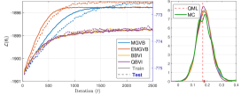
Figure 1: Lower bound optimization (left) and posterior distribution of for the $\gamma$ parameter (right). GJR-GARCH(1,1), Microsoft Inc. data.

II-C Transformations

It is clear that the application of Gaussian VI is problematic for the heavily constrained volatility models of Sec. II-A. For instance, a Gaussian posterior is incompatible with the $\omega>0$ or the $0<d<1$ requirements and plausibly with a Gaussian covariance structure (Gaussian copula). Moreover, the adoption of Gaussian priors is also inadequate. These issues can be fixed with appropriate parameter transforms.

In Algorithm 1, two steps are critical: (i) sampling from the Gaussian variational posterior and (ii) evaluating the model log-likelihood. By adopting the VI Gaussian framework, the unconstrained components of a sample ${\bm{\theta}}$ from $q_{{\bm{\zeta}}=\{{\bm{\mu}},\text{vec}(\Sigma)\}}$ need to be appropriately transformed into the valid constrained space for evaluating the log-likelihood. This is done, e.g., in [27] for the GARCH(1,1), and aligned with the well-adopted rationale for VI in medium-scale ML models of [14].

Let ${\bm{\nu}}$ denote a $d$-dimensional parameter parametrizing a GARCH-family model $m$, and $\mathcal{C}_{m}$ the constrained parameter space where ${\bm{\nu}}$ lives. Be $\psi_{m}:\mathcal{C}_{m}\mapsto\mathbb{R}^{d}$ a transform that maps ${\bm{\nu}}\in\mathcal{C}_{m}$ to ${\bm{\theta}}\in\mathbb{R}^{d}$. Let $\psi^{-1}_{m}$ denote the corresponding inverse transform, i.e., ${\bm{\nu}}=\psi^{-1}_{m}\left({\bm{\theta}}\right)$. This is the relevant transform in VI; we will show that such $\psi^{-1}_{m}$ exists and is of simple form for the models in Sec. II-A. Through $\psi^{-1}_{m}$ we can apply the update (4), map posterior samples ${\bm{\theta}}\sim q_{\bm{\zeta}}$ into $\mathcal{C}_{m}$ as $\psi^{-1}_{m}({\bm{\theta}})$, evaluate the likelihood, and approximate the expectation in (5). Similarly, we can, e.g., compare the QML estimates with the mean of transformed posterior samples, interpretable as approximations of the transformed posterior living in $\mathcal{C}_{m}$:

$$\mathbb{E}_{q_{{\bm{\zeta}}^{\star}}}\left[\psi^{-1}_{m}({\bm{\theta}}^{\star})\right]\approx\frac{1}{S}\sum_{s=1}^{S}\psi^{-1}_{m}({\bm{\theta}}^{\star}_{s}),\,{\bm{\theta}}^{\star}_{s}\sim q_{{\bm{\zeta}}^{\star}}\text{.}$$ (6)

In principle, QML could optimize $\ell(\psi^{-1}_{m}\left(\bm{\theta}\right))$, yet the use of constrained optimization is preponderant (e.g., in Python’s arch and R’s rugarch packages), so that parameter transforms are not relevant for standard QML estimation. Indeed, we are unaware of any work presenting such transformations. As fundamental for applying VI, and for future reference, we summarize them in the following propositions. For an element $\theta_{\lambda}$ of the vector ${\bm{\theta}}$ representing a certain parameter $\lambda$ of the model $m$, be ${\bm{\theta}}_{\lambda}$ its corresponding element in ${\bm{\theta}}$. Let $f$ denote the logistic function.

Proposition 1 (Inverse transforms for the FIGARCH)

The FIGARCH constraints $\omega>0$, $0\leq d\leq 1$, $0\leq\phi\leq(1-d)/2$, $0\leq\beta\leq d+\phi$, are satisfied by the following inverse transforms:

$$\omega=\exp(\theta_{\omega}), \qquad d=f(\theta_{d}),$$

$$\phi=f(\theta_{\phi})(1-d)/2, \qquad\beta=f(\omega_{\beta})\left(\phi+d\right).$$

Proof. The result follows immediately from [4, footnote 19].

Proposition 2 (Inverse transforms for the GJR-GARCH)

The GJR-GARCH(p,o,q) constraints $\omega>0$, $\alpha_{i}\geq 0$, $\sum\gamma_{k}+\sum\alpha_{i}\geq 0$, $\beta_{j}\geq 0$, $\sum(\alpha_{i}+1/2\gamma_{k}+\beta_{j})<1$, for $j=1,\dots,p$, $k=1,\dots,o$, $i=1,\dots,q$, for the GJR-GARCH(1,1) model are satisfied by the following inverse transforms:

$$\omega=exp\left(\theta_{\omega}\right), \qquad\alpha=f(\theta_{\alpha}),$$

$$\gamma=f(\theta_{\gamma})(2(1-\alpha)+\alpha)-\alpha, \qquad\beta=f(\theta_{\beta})\left(1-\alpha-1/2\gamma\right).$$

For the general GJR-GARCH$(p,o,q)$ case, inverse transforms can be computed as for Algorithm 2.

Proof. The transform for $\theta_{\omega}$ is obvious. As $\gamma$ and $\beta$ are still to be determined, the constraints imply that $\alpha$ can lay anywhere in $\left[0,1\right]$, so $\alpha=f(\omega_{\alpha})$. It is required that $\gamma+\alpha>0$, and $\alpha+\beta+1/2\gamma<1$. Yet $\beta$ is to be determined, so $1/2\gamma<1-\alpha$. The two give $-\alpha<\gamma<2(1-\alpha)$: we first map $\gamma$ to $[2(1-\alpha)+\alpha]$ and then shift the interval by $-\alpha$. I.e., $\gamma=f(\omega_{\gamma})[2(1-\alpha)+\alpha]-\alpha$. Now map $\theta_{\beta}$ in $1-\alpha-1/2\gamma$, that is $\beta=f(\omega_{\beta})(1-\alpha-1/2\gamma).$ With $p\geq 0,o\geq 0,q\geq 0$, the same interval-partitioning reasoning is sequentially repeated.

The last proposition applies to the ARCH ($o=p=0$) and GARCH models ($o=0)$ as a special case. Similarly, one can transform the possibly constrained trainable parameters of any postulated distribution for the iid $\{z_{i}\}$ innovations. For example, for a $GED\left(\lambda\right)$ distribution $\lambda=2+\theta_{\lambda}^{2}+\epsilon$, where $\epsilon>0$ is a pedestal to grant $\lambda>2$ holds strictly.

Algorithm 2 Inverse transformation for the $GJR(p,o,q)$

$\omega=\exp\left(\theta_{\omega}\right)$

$s=1-\varepsilon$

for $i=1,\dots,p$ do

     $\alpha_{i}=f\left(\theta_{\alpha_{i}}\right)s$

     $s=1-s$

end for

for $i=1,\dots,o$ do

     $\gamma_{i}=f\left(\theta_{\gamma_{i}}\right)$

     if $p\geq i$ then

         $\gamma_{i}=\left(2s+\alpha_{i}\right)\gamma_{i}-\alpha_{i}$

     else

         $\gamma_{i}=2s\gamma_{i}$

     end if

     $s=1-0.5s$

end for

for $i=1,\dots,q$ do

     $\beta_{i}=f(\theta_{\beta_{i}})$

     $s=1-s$

end for

III Experiments

III-A Data

For our empirical analyses, we use daily close-to-close log returns for the constituents of the S&P500 index. Our data covers 1383 trading days, from 1 January 2018 to 30 June 2023, divided into train and test sets with a 75%-25% split following chronological order. We use 488 stocks, since some constituents changed and their time series are incomplete.

III-B Models, and optimization

To assess how satisfactory VI is in volatility modeling, we adopt the following volatility models: ARCH(1), GARCH(1,1), GJR-GARCH(1,1), EGARCH(0,1), EGARCH(1,1), GJR-EGARCH(1,1), FIGARCH(1,d,1). The case study on the Microsoft Corp. data additionally includes the GARCH(2,1), EGARCH(2,1), and the FIGARCH(0,d,1). The analyses adopt the BBVI, QBVI, MGVB, and EMGVB optimizers for VI (the first two under a diagonal variational covariance matrix). For the FIGARCH models, we implement (1) by the method of [23]. As a baseline for comparison, we adopt QML estimates and a Monte Carlo Markov Chain Sampler (MC). An MC reference for VI is advisable as it provides a benchmark for highlighting biases and assessing the quality of the Gaussian variational approximation.

For consistency, in VI, we adopt the same set of hyperparameters for all the experiments and optimizers. In particular, we use a learning rate of $0.005$, $50$ MC draws for approximating the expectation (5), a diagonal normal prior of unit variance and initial values ${\bm{\mu}}_{0}=0$, $\Sigma_{0}=0.1I$. To increase the stability of the learning process, we update the gradients with a momentum factor of $0.4$. Both MC and VI algorithms are run for a longer-than-required number of iterations. This avoids tuning the parameter on a case-by-case basis (which is unfeasible with hundreds of stocks) and provides reasonable guarantees that the algorithms converged. For VI, we observe that typically 1500 iterations are sufficient for the LB to reach a plateau (Fig. 1), yet we terminate the training after 2500 iterations. Opposed to ML, in statistics overfitting is a major concern in model selection. For example, in maximum likelihood estimation, the dynamic of the likelihood on a (usually nonexistent) test set is ignored. Early-stopping criteria for MC/VI based on the test loss would lead to non-comparability with the fully-in-sample-optimized maximum likelihood estimates. The relevant data and codes for the experiments are available at github.com/mmagris/GARCHVI.

III-C Results

III-C1 General results

To assess the effectiveness of VI as a Bayesian procedure, we adopt four performance metrics on the training and test sets. For VI, performances are computed as averages of $7,000$ inversely-transformed samples from the estimated variational posterior $q_{{\bm{\zeta}}^{\star}}\left({\bm{\theta}}\right)$. For MC, the last $7,000$ samples of the Markov chain. The metrics are the Negative Log-Likelihood (NLL), the Root Mean Squared Error (RMSE), the Mean Absolute Deviation (MAD), and the Qlik loss [24]. For the last three, as proxies for the observed conditional variances, we adopt squared returns [24].

TABLE I: Main estimation results. Averages and respective standard deviations across the S&P 500 stocks, of the differences between the individual estimators’ performance with respect to the QML performance, expressed as a percentage of the QML performance. Performances are evaluated in the transformed posterior mean (6).

	Train				Test
	RMSE	MAD	QLIK	NLL	RMSE	MAD	QLIK	NLL
ARCH(1)
MCMC	+0.257$\pm$35.820	+0.488$\pm$42.559	+0.105$\pm$1.306	+0.045$\pm$0.750	+0.422$\pm$40.208	+0.562$\pm$51.238	+0.128$\pm$18.353	+0.048$\pm$6.264
MGVB	+0.308$\pm$39.794	+0.555$\pm$41.888	+0.113$\pm$1.476	+0.048$\pm$0.745	+0.525$\pm$41.932	+0.663$\pm$52.409	+0.175$\pm$20.910	+0.066$\pm$7.305
EMGVB	+0.313$\pm$39.756	+0.562$\pm$41.596	+0.113$\pm$1.474	+0.048$\pm$0.745	+0.532$\pm$41.673	+0.670$\pm$52.077	+0.176$\pm$20.927	+0.066$\pm$7.304
BBVI	+0.313$\pm$39.755	+0.562$\pm$41.594	+0.113$\pm$1.474	+0.048$\pm$0.745	+0.532$\pm$41.671	+0.670$\pm$52.075	+0.176$\pm$20.927	+0.066$\pm$7.304
QBVI	+0.277$\pm$37.496	+0.532$\pm$40.190	+0.116$\pm$1.464	+0.049$\pm$0.744	+0.502$\pm$37.718	+0.639$\pm$50.450	+0.181$\pm$19.112	+0.067$\pm$7.027
GARCH(1,1)
MCMC	+0.008$\pm$57.547	+0.033$\pm$126.751	+0.279$\pm$8.379	+0.111$\pm$3.371	+0.378$\pm$45.971	+0.320$\pm$117.589	+0.218$\pm$77.296	+0.080$\pm$30.211
MGVB	-0.019$\pm$56.563	+0.118$\pm$122.241	+0.265$\pm$7.860	+0.106$\pm$3.149	+0.394$\pm$44.033	+0.431$\pm$112.530	+0.221$\pm$73.356	+0.081$\pm$28.555
EMGVB	-0.016$\pm$56.838	+0.129$\pm$123.087	+0.268$\pm$7.888	+0.107$\pm$3.170	+0.399$\pm$44.328	+0.441$\pm$113.424	+0.223$\pm$73.864	+0.082$\pm$28.690
BBVI	-0.016$\pm$56.843	+0.129$\pm$123.097	+0.268$\pm$7.889	+0.107$\pm$3.171	+0.399$\pm$44.333	+0.441$\pm$113.433	+0.223$\pm$73.869	+0.082$\pm$28.692
QBVI	-0.098$\pm$40.651	+0.048$\pm$107.369	+0.225$\pm$5.025	+0.090$\pm$1.882	+0.270$\pm$32.590	+0.355$\pm$97.150	+0.244$\pm$47.097	+0.091$\pm$18.423
GJR-GARCH(1,1)
MCMC	+0.216$\pm$136.296	+1.076$\pm$188.896	+0.498$\pm$19.800	+0.198$\pm$8.189	+1.023$\pm$110.649	+1.350$\pm$206.975	+0.207$\pm$155.432	+0.079$\pm$60.732
MGVB	+0.191$\pm$131.465	+0.889$\pm$186.580	+0.509$\pm$19.616	+0.202$\pm$8.006	+0.959$\pm$105.886	+1.140$\pm$204.363	+0.226$\pm$154.253	+0.084$\pm$59.804
EMGVB	+0.173$\pm$119.290	+0.903$\pm$189.253	+0.513$\pm$20.138	+0.204$\pm$8.280	+0.972$\pm$109.063	+1.151$\pm$207.438	+0.235$\pm$156.458	+0.088$\pm$60.738
BBVI	+0.173$\pm$119.297	+0.903$\pm$189.261	+0.513$\pm$20.140	+0.204$\pm$8.281	+0.972$\pm$109.076	+1.151$\pm$207.446	+0.235$\pm$156.471	+0.088$\pm$60.744
QBVI	-0.041$\pm$83.022	+0.727$\pm$154.161	+0.408$\pm$12.397	+0.162$\pm$4.942	+0.580$\pm$66.795	+0.998$\pm$163.206	+0.169$\pm$103.345	+0.066$\pm$40.164
EGARCH(0,1)
MCMC	+0.591$\pm$100.969	+0.447$\pm$47.094	+0.099$\pm$0.889	+0.043$\pm$0.509	+0.277$\pm$35.295	+0.278$\pm$26.375	+0.079$\pm$4.951	+0.029$\pm$1.776
MGVB	+0.704$\pm$119.838	+0.418$\pm$49.920	+0.111$\pm$0.935	+0.048$\pm$0.540	+0.335$\pm$49.310	+0.234$\pm$31.721	+0.111$\pm$9.794	+0.041$\pm$3.327
EMGVB	+0.667$\pm$113.577	+0.400$\pm$50.086	+0.107$\pm$0.870	+0.046$\pm$0.524	+0.320$\pm$47.369	+0.216$\pm$30.581	+0.108$\pm$9.811	+0.040$\pm$3.336
BBVI	+0.667$\pm$113.588	+0.400$\pm$50.089	+0.107$\pm$0.870	+0.046$\pm$0.524	+0.320$\pm$47.373	+0.216$\pm$30.584	+0.108$\pm$9.811	+0.040$\pm$3.336
QBVI	+0.591$\pm$99.846	+0.338$\pm$46.964	+0.106$\pm$0.864	+0.046$\pm$0.518	+0.258$\pm$38.595	+0.163$\pm$29.894	+0.104$\pm$10.196	+0.039$\pm$3.497
EGARCH(1,1)
MCMC	+0.174$\pm$28.495	+0.450$\pm$33.825	+0.199$\pm$1.921	+0.080$\pm$1.076	+0.244$\pm$28.261	+0.501$\pm$57.923	+0.216$\pm$33.674	+0.079$\pm$12.473
MGVB	+0.131$\pm$30.125	+0.533$\pm$31.338	+0.198$\pm$3.107	+0.079$\pm$1.237	+0.276$\pm$31.356	+0.609$\pm$54.202	+0.237$\pm$33.555	+0.085$\pm$12.823
EMGVB	+0.455$\pm$68.170	+0.708$\pm$83.257	+0.622$\pm$40.371	+0.240$\pm$13.503	+0.571$\pm$63.156	+0.809$\pm$169.018	+0.625$\pm$97.310	+0.224$\pm$35.607
BBVI	+0.456$\pm$68.614	+0.724$\pm$83.494	+0.623$\pm$40.489	+0.241$\pm$13.556	+0.577$\pm$63.868	+0.807$\pm$164.302	+0.626$\pm$97.604	+0.225$\pm$35.741
QBVI	+0.397$\pm$76.614	+0.998$\pm$99.027	+0.748$\pm$49.880	+0.288$\pm$16.616	+0.745$\pm$84.246	+1.375$\pm$178.473	+0.749$\pm$115.469	+0.261$\pm$39.564
GJR-EGARCH(1,1)
MCMC	+0.165$\pm$38.646	+0.785$\pm$44.847	+0.259$\pm$2.923	+0.103$\pm$1.644	+0.406$\pm$47.171	+0.849$\pm$83.595	+0.259$\pm$41.236	+0.094$\pm$14.483
MGVB	+0.202$\pm$56.358	+0.819$\pm$54.540	+0.310$\pm$9.159	+0.127$\pm$4.050	+0.465$\pm$53.650	+0.929$\pm$112.795	+0.310$\pm$60.818	+0.114$\pm$21.561
EMGVB	+0.846$\pm$107.619	+1.214$\pm$120.063	+1.026$\pm$71.257	+0.394$\pm$24.872	+1.043$\pm$146.509	+1.124$\pm$272.713	+0.781$\pm$161.688	+0.276$\pm$55.370
BBVI	+0.847$\pm$108.432	+1.235$\pm$120.755	+1.028$\pm$71.166	+0.394$\pm$24.853	+1.047$\pm$146.676	+1.150$\pm$273.753	+0.783$\pm$162.340	+0.277$\pm$55.636
QBVI	+0.828$\pm$139.379	+1.831$\pm$153.957	+1.170$\pm$79.713	+0.449$\pm$27.667	+1.412$\pm$187.324	+2.177$\pm$324.510	+0.897$\pm$175.608	+0.326$\pm$64.718
FIGARCH(1,d,1)
MCMC	+0.090$\pm$54.384	+0.845$\pm$136.805	+0.258$\pm$15.436	+0.103$\pm$6.538	+0.204$\pm$48.465	+1.007$\pm$205.486	-0.028$\pm$64.930	-0.018$\pm$25.460
MGVB	+0.146$\pm$59.358	+2.381$\pm$217.490	+0.149$\pm$21.112	+0.061$\pm$8.566	+0.475$\pm$67.696	+2.620$\pm$277.691	-0.587$\pm$101.008	-0.213$\pm$36.897
EMGVB	+0.172$\pm$68.563	+2.477$\pm$240.598	+0.153$\pm$21.398	+0.063$\pm$8.714	+0.514$\pm$76.643	+2.762$\pm$307.879	-0.569$\pm$105.048	-0.206$\pm$38.216
BBVI	+0.172$\pm$68.730	+2.478$\pm$240.930	+0.153$\pm$21.404	+0.063$\pm$8.717	+0.514$\pm$76.825	+2.764$\pm$308.238	-0.569$\pm$105.073	-0.206$\pm$38.222
QBVI	+0.145$\pm$58.516	+2.427$\pm$217.864	+0.168$\pm$20.448	+0.069$\pm$8.299	+0.493$\pm$67.799	+2.716$\pm$301.438	-0.577$\pm$99.190	-0.209$\pm$36.377

Table I presents the overall estimation results for the 488 stocks. For a performance metric $M_{E}^{x}$ computed on a data subsample $x$ as a result of an estimation procedure $E$, the entries in the Table correspond to mean performance deviations from the QML benchmark expressed as percentages, i.e., $100(M^{x}_{E}/M^{x}_{QML}-1)$, and their standard deviations for the S&P 500 stocks. We comment on the predominance of positive signs indicating that QML is, overall, the preferred estimation approach from a merely quantitative perspective. However, VI methods can sometimes outperform QML in certain model/loss combinations. Clearly, test NLL values are always positive, confirming that QML estimates are optimal in this sense. At a general level, the typical magnitude of the ratios is in the sub-1% order, indicating that MC/VI estimation procedures are indeed effective w.r.t. QML and each other. Among the VI optimizers, we do not observe patterns indicating the dominance of one optimizer over another, implying they all determine a comparable variational approximation and, thus, performance. At the same time, the homogeneity in the results indicates that VI is robust with respect to the choice of the optimizer; all the optimizers appear adequate for the problems analyzed. By applying Chebyshev’s inequality with, e.g., a margin of 3 standard deviations, the differences are broadly insignificant, indicating that the Gaussian variational approximation for the unconstrained parameters is plausible, at least for capturing the first two moments of the margins.

Regardless of the VI optimizer and volatility model, these results show that VI firmly stands as a valid estimation alternative to MC sampling. The in-sample and out-of-sample loss in performance w.r.t. QML is negligible, while the Bayesian framework enables several advantages, as for Sec. I.

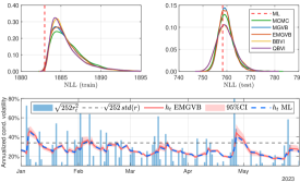
Figure 2: Distribution of the train (top left) and test (top right) NNL, and confidence bounds for the conditional volatility (bottom). GJR-GARCH(1,1), Microsoft Inc. data.

III-C2 Case study

We provide further analyses for Microsoft Corp. data. Table II summarizes the results regarding the training processes and the parameters’ estimates.

TABLE II: Estimation results for the Microsoft Inc. data for the GJR-GARCH(1,1). Differences with respect to the QML estimates and standard deviations. Parameter estimates refer to transformed posterior means (6), while performances’ means and standard deviations are computed from transformed posterior samples.

	Parameters				Train		Test		Train			Test
	$\omega$	$\alpha$			$\mathcal{L}(\bf{\theta}^{\star})$	$p(y|\bf{\theta}^{\star})$	$\mathcal{L}(\bf{\theta}^{\star})$	$p(y|\bf{\theta}^{\star})$	RMSE	QLIK	NLL	RMSE	QLIK	NLL
ARCH(1)
ML	1.92	0.43				-1966.75		-770.55	10.04	1.67	1966.75	8.49	1.58	770.55
MCMC	1.905$\pm$0.117	0.446$\pm$0.066				-1966.77		-770.64	10.040$\pm$0.131	1.670$\pm$0.002	1967.688$\pm$0.914	8.548$\pm$0.193	1.579$\pm$0.024	770.981$\pm$4.151
MGVB	1.904$\pm$0.121	0.446$\pm$0.066			-1971.19	-1966.77	-774.44	-770.68	10.040$\pm$0.137	1.670$\pm$0.002	1967.726$\pm$0.930	8.549$\pm$0.191	1.579$\pm$0.025	771.049$\pm$4.281
EMGVB	1.904$\pm$0.122	0.446$\pm$0.066			-1971.19	-1966.77	-774.44	-770.69	10.041$\pm$0.138	1.670$\pm$0.002	1967.731$\pm$0.972	8.547$\pm$0.190	1.579$\pm$0.025	771.043$\pm$4.307
BBVI	1.907$\pm$0.108	0.445$\pm$0.057			-1971.32	-1966.77	-774.53	-770.60	10.036$\pm$0.120	1.670$\pm$0.002	1967.749$\pm$1.097	8.541$\pm$0.161	1.579$\pm$0.027	771.028$\pm$4.582
QBVI	1.905$\pm$0.108	0.446$\pm$0.057			-1971.32	-1966.77	-774.55	-770.63	10.034$\pm$0.120	1.670$\pm$0.002	1967.741$\pm$1.100	8.545$\pm$0.162	1.579$\pm$0.027	771.062$\pm$4.557
GARCH(1,1)			$\beta$
ML	0.15	0.19	0.77			-1890.44		-761.47	10.51	1.52	1890.44	8.09	1.52	761.42
MCMC	0.200$\pm$0.046	0.203$\pm$0.031	0.737$\pm$0.036			-1890.98		-762.31	10.446$\pm$0.072	1.523$\pm$0.003	1892.321$\pm$1.502	8.117$\pm$0.067	1.532$\pm$0.015	762.932$\pm$2.539
MGVB	0.205$\pm$0.047	0.201$\pm$0.030	0.736$\pm$0.035		-1901.36	-1891.06	-771.91	-762.49	10.444$\pm$0.071	1.523$\pm$0.003	1892.456$\pm$1.715	8.111$\pm$0.061	1.532$\pm$0.017	762.999$\pm$2.912
EMGVB	0.205$\pm$0.047	0.201$\pm$0.029	0.736$\pm$0.035		-1901.36	-1891.06	-771.90	-762.51	10.444$\pm$0.071	1.523$\pm$0.003	1892.446$\pm$1.698	8.111$\pm$0.061	1.532$\pm$0.017	763.017$\pm$2.910
BBVI	0.196$\pm$0.021	0.199$\pm$0.023	0.740$\pm$0.023		-1902.27	-1890.89	-772.87	-762.55	10.449$\pm$0.048	1.523$\pm$0.003	1892.334$\pm$1.740	8.106$\pm$0.049	1.532$\pm$0.022	762.995$\pm$3.708
QBVI	0.197$\pm$0.020	0.199$\pm$0.023	0.740$\pm$0.023		-1902.27	-1890.92	-772.88	-762.60	10.449$\pm$0.048	1.523$\pm$0.003	1892.387$\pm$1.783	8.105$\pm$0.049	1.532$\pm$0.022	762.939$\pm$3.769
GARCH(2,1)			$\beta_{1}$	$\beta_{2}$
ML	0.17	0.21	0.62	0.13		-1890.26		-761.03	10.43	1.52	1890.26	8.09	1.52	760.99
MCMC	0.209$\pm$0.052	0.231$\pm$0.038	0.545$\pm$0.117	0.160$\pm$0.092		-1890.65		-762.61	10.372$\pm$0.086	1.522$\pm$0.003	1892.089$\pm$1.381	8.140$\pm$0.077	1.527$\pm$0.015	762.110$\pm$2.589
MGVB	0.212$\pm$0.051	0.229$\pm$0.035	0.543$\pm$0.100	0.164$\pm$0.080	-1898.50	-1890.59	-768.27	-762.10	10.372$\pm$0.084	1.522$\pm$0.003	1892.104$\pm$1.566	8.134$\pm$0.071	1.526$\pm$0.018	761.916$\pm$3.031
EMGVB	0.211$\pm$0.053	0.230$\pm$0.035	0.543$\pm$0.103	0.164$\pm$0.083	-1898.49	-1890.59	-768.27	-762.12	10.371$\pm$0.085	1.522$\pm$0.003	1892.127$\pm$1.581	8.135$\pm$0.071	1.526$\pm$0.018	761.918$\pm$3.010
BBVI	0.204$\pm$0.022	0.229$\pm$0.025	0.555$\pm$0.047	0.159$\pm$0.034	-1900.28	-1890.50	-769.82	-761.34	10.372$\pm$0.056	1.523$\pm$0.005	1892.379$\pm$2.315	8.134$\pm$0.055	1.526$\pm$0.026	761.997$\pm$4.391
QBVI	0.205$\pm$0.022	0.230$\pm$0.024	0.552$\pm$0.047	0.161$\pm$0.034	-1900.27	-1890.50	-769.85	-761.33	10.370$\pm$0.056	1.523$\pm$0.005	1892.384$\pm$2.329	8.134$\pm$0.053	1.526$\pm$0.026	762.071$\pm$4.394
GJR-GARCH(1,1)			$\gamma$	$\beta$
ML	0.17	0.09	0.17	0.77		-1882.96		-758.24	10.59	1.50	1882.96	8.02	1.50	758.18
MCMC	0.218$\pm$0.046	0.111$\pm$0.031	0.182$\pm$0.056	0.731$\pm$0.034		-1883.76		-759.25	10.560$\pm$0.071	1.510$\pm$0.004	1885.662$\pm$1.819	8.089$\pm$0.075	1.517$\pm$0.017	760.414$\pm$2.902
MGVB	0.218$\pm$0.045	0.111$\pm$0.031	0.182$\pm$0.050	0.731$\pm$0.035	-1897.75	-1883.77	-772.49	-759.43	10.556$\pm$0.060	1.509$\pm$0.004	1885.575$\pm$1.906	8.088$\pm$0.070	1.516$\pm$0.018	760.344$\pm$3.151
EMGVB	0.218$\pm$0.047	0.111$\pm$0.030	0.182$\pm$0.051	0.730$\pm$0.035	-1897.74	-1883.77	-772.48	-759.42	10.557$\pm$0.061	1.510$\pm$0.004	1885.590$\pm$1.889	8.088$\pm$0.070	1.516$\pm$0.018	760.350$\pm$3.081
BBVI	0.212$\pm$0.021	0.112$\pm$0.028	0.178$\pm$0.048	0.733$\pm$0.022	-1898.68	-1883.65	-773.50	-759.57	10.550$\pm$0.051	1.509$\pm$0.004	1885.548$\pm$1.997	8.080$\pm$0.052	1.516$\pm$0.024	760.368$\pm$4.023
QBVI	0.209$\pm$0.020	0.111$\pm$0.029	0.177$\pm$0.049	0.735$\pm$0.022	-1898.69	-1883.60	-773.42	-759.44	10.551$\pm$0.052	1.509$\pm$0.004	1885.490$\pm$1.985	8.078$\pm$0.051	1.516$\pm$0.024	760.263$\pm$4.038
EGARCH(0,1)
ML	1.12	0.50				-1999.77		-758.82	11.68	1.73	1999.77	8.07	1.51	758.82
MCMC	1.121$\pm$0.052	0.502$\pm$0.050				-1999.77		-758.86	11.694$\pm$0.025	1.735$\pm$0.002	2000.717$\pm$0.916	8.091$\pm$0.081	1.510$\pm$0.020	759.203$\pm$3.378
MGVB	1.121$\pm$0.053	0.501$\pm$0.050			-2006.49	-1999.77	-764.15	-758.85	11.695$\pm$0.027	1.735$\pm$0.002	2000.757$\pm$0.972	8.091$\pm$0.081	1.510$\pm$0.021	759.222$\pm$3.511
EMGVB	1.121$\pm$0.053	0.501$\pm$0.050			-2006.49	-1999.77	-764.23	-758.85	11.694$\pm$0.027	1.735$\pm$0.002	2000.745$\pm$0.996	8.090$\pm$0.080	1.510$\pm$0.020	759.194$\pm$3.493
BBVI	1.120$\pm$0.051	0.500$\pm$0.048			-2006.52	-1999.77	-764.31	-758.87	11.694$\pm$0.024	1.735$\pm$0.002	2000.761$\pm$1.039	8.088$\pm$0.080	1.510$\pm$0.022	759.202$\pm$3.780
QBVI	1.120$\pm$0.051	0.500$\pm$0.048			-2006.52	-1999.77	-764.51	-758.87	11.694$\pm$0.024	1.735$\pm$0.002	2000.765$\pm$1.050	8.087$\pm$0.080	1.510$\pm$0.023	759.209$\pm$3.837
EGARCH(1,1)			$\beta$
ML	0.07	0.35	0.94			-1893.86		-754.74	10.49	1.53	1893.86	7.97	1.48	754.74
MCMC	0.076$\pm$0.018	0.371$\pm$0.044	0.933$\pm$0.016			-1893.95		-755.12	10.480$\pm$0.105	1.529$\pm$0.002	1895.328$\pm$1.243	8.001$\pm$0.060	1.487$\pm$0.012	755.318$\pm$2.055
MGVB	0.076$\pm$0.017	0.368$\pm$0.044	0.933$\pm$0.016		-1906.51	-1893.94	-766.16	-755.04	10.488$\pm$0.110	1.529$\pm$0.003	1895.409$\pm$1.287	7.997$\pm$0.057	1.487$\pm$0.012	755.263$\pm$2.128
EMGVB	0.082$\pm$0.021	0.382$\pm$0.047	0.927$\pm$0.019		-1906.63	-1894.18	-766.23	-755.34	10.478$\pm$0.122	1.530$\pm$0.003	1895.999$\pm$1.689	8.012$\pm$0.065	1.489$\pm$0.014	755.647$\pm$2.423
BBVI	0.093$\pm$0.011	0.399$\pm$0.039	0.917$\pm$0.010		-1907.75	-1894.75	-767.06	-755.52	10.461$\pm$0.115	1.531$\pm$0.003	1896.368$\pm$1.762	8.024$\pm$0.061	1.490$\pm$0.018	755.929$\pm$3.039
QBVI	0.096$\pm$0.011	0.403$\pm$0.039	0.915$\pm$0.011		-1907.92	-1894.94	-767.06	-755.55	10.457$\pm$0.117	1.531$\pm$0.004	1896.681$\pm$1.945	8.029$\pm$0.063	1.490$\pm$0.019	755.898$\pm$3.170
EGARCH(2,1)			$\beta_{1}$	$\beta_{2}$
ML	0.07	0.38	0.85	0.09		-1893.73		-754.23	10.47	1.53	1893.73	7.97	1.48	754.23
MCMC	0.079$\pm$0.020	0.395$\pm$0.058	0.813$\pm$0.152	0.117$\pm$0.147		-1893.81		-754.54	10.483$\pm$0.115	1.529$\pm$0.003	1895.766$\pm$1.553	8.008$\pm$0.077	1.486$\pm$0.014	755.107$\pm$2.330
MGVB	0.079$\pm$0.018	0.392$\pm$0.053	0.813$\pm$0.141	0.118$\pm$0.138	-1908.04	-1893.80	-767.03	-754.29	10.485$\pm$0.115	1.529$\pm$0.003	1895.665$\pm$1.459	8.002$\pm$0.063	1.484$\pm$0.013	754.826$\pm$2.281
EMGVB	0.093$\pm$0.025	0.419$\pm$0.055	0.799$\pm$0.103	0.118$\pm$0.099	-1908.55	-1894.32	-767.41	-755.00	10.466$\pm$0.136	1.531$\pm$0.004	1896.708$\pm$2.066	8.029$\pm$0.077	1.488$\pm$0.016	755.544$\pm$2.774
BBVI	0.111$\pm$0.013	0.443$\pm$0.043	0.829$\pm$0.013	0.074$\pm$0.012	-1912.81	-1895.66	-770.53	-755.37	10.431$\pm$0.138	1.534$\pm$0.006	1898.215$\pm$3.089	8.063$\pm$0.083	1.491$\pm$0.023	756.064$\pm$3.852
QBVI	0.111$\pm$0.013	0.447$\pm$0.043	0.817$\pm$0.014	0.085$\pm$0.013	-1912.87	-1895.68	-770.48	-755.45	10.433$\pm$0.140	1.535$\pm$0.007	1898.410$\pm$3.372	8.065$\pm$0.081	1.493$\pm$0.024	756.304$\pm$4.079
GJR-EGARCH(1,1)			$\gamma$	$\beta$
ML	0.07	0.30	-0.10	0.94		-1885.35		-749.47	10.52	1.51	1885.35	7.91	1.45	749.47
MCMC	0.073$\pm$0.016	0.319$\pm$0.047	-0.105$\pm$0.025	0.931$\pm$0.015		-1885.47		-750.24	10.526$\pm$0.105	1.513$\pm$0.003	1887.398$\pm$1.465	7.945$\pm$0.072	1.460$\pm$0.014	750.668$\pm$2.437
MGVB	0.074$\pm$0.016	0.320$\pm$0.045	-0.106$\pm$0.026	0.930$\pm$0.015	-1901.83	-1885.47	-764.69	-750.01	10.521$\pm$0.102	1.513$\pm$0.003	1887.407$\pm$1.454	7.944$\pm$0.061	1.458$\pm$0.014	750.435$\pm$2.368
EMGVB	0.084$\pm$0.021	0.342$\pm$0.049	-0.108$\pm$0.031	0.921$\pm$0.019	-1902.11	-1885.95	-764.90	-750.65	10.514$\pm$0.112	1.515$\pm$0.004	1888.489$\pm$1.990	7.977$\pm$0.079	1.463$\pm$0.016	751.266$\pm$2.764
BBVI	0.095$\pm$0.010	0.357$\pm$0.039	-0.113$\pm$0.028	0.911$\pm$0.010	-1903.33	-1886.69	-766.01	-750.98	10.511$\pm$0.109	1.516$\pm$0.004	1888.890$\pm$2.033	7.998$\pm$0.081	1.465$\pm$0.019	751.582$\pm$3.324
QBVI	0.098$\pm$0.011	0.363$\pm$0.039	-0.114$\pm$0.028	0.908$\pm$0.011	-1903.58	-1886.97	-765.99	-751.10	10.511$\pm$0.111	1.517$\pm$0.004	1889.281$\pm$2.176	8.009$\pm$0.087	1.466$\pm$0.021	751.790$\pm$3.531
FIGARCH(0,$d$,1)		$d$	$\beta$
ML	0.28	0.47	0.25			-1891.66		-759.11	10.40	1.52	1891.66	8.15	1.51	759.11
MCMC	0.303$\pm$0.086	0.511$\pm$0.115	0.275$\pm$0.133			-1891.64		-759.08	10.447$\pm$0.190	1.524$\pm$0.002	1892.831$\pm$1.070	8.180$\pm$0.080	1.511$\pm$0.010	759.519$\pm$1.718
MGVB	0.340$\pm$0.083	0.523$\pm$0.094	0.290$\pm$0.109		-1895.55	-1891.54	-761.56	-758.34	10.454$\pm$0.174	1.524$\pm$0.002	1892.737$\pm$1.164	8.193$\pm$0.081	1.507$\pm$0.010	758.735$\pm$1.628
EMGVB	0.340$\pm$0.081	0.523$\pm$0.094	0.291$\pm$0.110		-1895.55	-1891.54	-761.57	-758.34	10.454$\pm$0.176	1.523$\pm$0.002	1892.735$\pm$1.149	8.193$\pm$0.081	1.507$\pm$0.010	758.727$\pm$1.622
BBVI	0.333$\pm$0.072	0.493$\pm$0.058	0.266$\pm$0.054		-1896.15	-1891.54	-761.65	-758.10	10.421$\pm$0.136	1.524$\pm$0.003	1892.916$\pm$1.548	8.182$\pm$0.093	1.505$\pm$0.011	758.442$\pm$1.921
QBVI	0.330$\pm$0.072	0.490$\pm$0.057	0.262$\pm$0.053		-1896.15	-1891.54	-761.66	-758.15	10.419$\pm$0.135	1.524$\pm$0.003	1892.944$\pm$1.550	8.179$\pm$0.093	1.505$\pm$0.011	758.444$\pm$1.952
FIGARCH(1,$d$,1)		$\phi$	$d$	$\beta$
ML	0.30	0.15	0.58	0.50		-1890.83		-758.83	10.41	1.52	1890.83	8.17	1.51	758.83
MCMC	0.307$\pm$0.091	0.112$\pm$0.055	0.549$\pm$0.124	0.412$\pm$0.122		-1891.06		-758.97	10.395$\pm$0.173	1.523$\pm$0.002	1892.431$\pm$1.245	8.191$\pm$0.083	1.511$\pm$0.010	759.438$\pm$1.723
MGVB	0.343$\pm$0.082	0.108$\pm$0.048	0.573$\pm$0.106	0.438$\pm$0.104	-1895.36	-1890.93	-761.87	-758.37	10.427$\pm$0.158	1.522$\pm$0.002	1892.201$\pm$1.209	8.197$\pm$0.083	1.507$\pm$0.010	758.759$\pm$1.657
EMGVB	0.343$\pm$0.083	0.107$\pm$0.049	0.573$\pm$0.108	0.437$\pm$0.105	-1895.35	-1890.93	-761.85	-758.37	10.426$\pm$0.159	1.523$\pm$0.002	1892.232$\pm$1.211	8.198$\pm$0.082	1.507$\pm$0.010	758.763$\pm$1.645
BBVI	0.341$\pm$0.070	0.112$\pm$0.047	0.567$\pm$0.075	0.444$\pm$0.061	-1895.88	-1890.89	-761.95	-758.14	10.435$\pm$0.122	1.523$\pm$0.003	1892.388$\pm$1.651	8.190$\pm$0.092	1.505$\pm$0.012	758.449$\pm$2.056
QBVI	0.341$\pm$0.071	0.113$\pm$0.048	0.560$\pm$0.073	0.437$\pm$0.060	-1895.89	-1890.91	-761.92	-758.09	10.426$\pm$0.123	1.523$\pm$0.003	1892.368$\pm$1.561	8.188$\pm$0.090	1.505$\pm$0.012	758.401$\pm$2.016

The takeaway, justified blow, is that differences in performance metrics are broadly negligible, and the differences in the estimated parameters are minor. The impact of the chosen estimation method is secondary, promoting VI as a solid alternative to MC and QML. Performance metrics are broadly overlapping, and differences are not statistically different except for the train NLL, consistently minimized by QML.

It is instructive to look at the performance metrics achieved by the different optimizers. For all the models, the MSFT findings align with the percentage reported in Table I. On both the training and test sets, the values of the performance metrics are remarkably aligned between QML and the Bayesian estimators, also for the additional models. Switching to a Bayesian framework does not harm with respect to QML performance on both sets. The estimated variance indicates broad non-significance in the difference across the Bayesian estimates, if not for $NLL^{\text{train}}$. We do not include the additional table with all the cross-testing results but rather visually discuss this case in Figure 2. The top-right panel of Figure 2 shows that the hypothesis $NLL_{QML}^{\text{train}}=NLL_{VI}^{\text{train}}$ cannot be rejected. Conversely, its rejection on the training set validates the above.

Extending the analysis to the value of the optimized LB, we observe that all the VI optimizers are rather equivalent for Bayesian inference, targeting a similar optimum. Clearly, the diagonal BBVI and QBVI ones do not reach the same LB optimum that MGVB and EMGVB do (see. e.g., the GJR-GARCH(1,1) case in Table II and Figure 1), yet the differences are well within $1\%$, both on the training and test sets. The differences in the LB correspond to differences in the posterior estimates, explaining differences in the estimates posterior means of Table II. Yet, performance metrics are practically analogous; all the reported estimates can be considered equally effective, especially for out-of-sample forecasting.

In this regard, we observe a remarkable alignment between the MC and MGVB/EMGVB estimates and the standard deviations, suggesting that the full-covariance Gaussian specification appears feasible, at least for capturing the first two moments of the marginal distribution of the true posterior (approximated by the MC sampler). Figure 1 includes the posterior means for the GJR-GARCH(1,1) model in the constrained parameter space. The plot highlights the importance of allowing for a full-covariance specification, and the MGVB/EMGVB overlap to the MC density supports the Gaussian variational framework. Observing the QML estimates within the region of high density further validates the overall VI calibration with respect to QML.

As an example of how VI could provide additional insights with respect to the standard frequentist approach, the bottom panel of Figure 2 shows confidence bounds for the predicted conditional variance for 2023. Enabling a probabilistic dimension for the conditional variance can certainly benefit financial practitioners [1, Ch. 6]). For instance, by enabling statistical testing (e.g., for tomorrow’s variance being significantly higher than today’s), or improving value-at-risk density evaluations, as for Sec. I. Our results indicate that VI can serve this scope well.

III-D Robustness checks

Tables III and IV further validate our study by addressing the effect different distributions for the iid innovations $\{z_{t}\}$ and prior variances have on the estimates. The reported results involve the MGVB optimizer, the GJR-GARCH(1,1) model, and at the estimated parameter only. In Table III, we consider four distributions and include the corresponding parameters as trainable parameters. The results across the sections of Table III are consistent and robust. The remarkably small ratios in Table I are perhaps not related to the choice of the innovations’ distribution but rather to the robustness of the VI setup in this setting.

Small prior variance does affect the posterior estimation by keeping the posterior mean rather away from the QML estimates (see Table IV). This is certainly positive if one has motivated prior beliefs on the parameter in the unconstrained space (though unlikely). On the other hand, prior variances greater than one already deliver similar estimates (further aligned with QML). Encoding prior lack of knowledge appears to be relatively smooth; a prior variance $\tau I$ with $\tau>1$ is effective in this regard.

TABLE III: Estimation results under different parametric forms of the iid innovations. Microsoft Inc. data, GJR-GARCH(1,1).

Error	Optimizer	$\omega$	$\alpha$	$\gamma$	$\beta$	$\nu$	$\lambda$
Normal	ML	0.169	0.089	0.169	0.772
	MCMC	0.218	0.111	0.182	0.731
	EMGVB	0.218	0.111	0.182	0.730
Student-t	ML	0.148	0.067	0.203	0.788	6.991
	MCMC	0.236	0.106	0.226	0.720	6.417
	EMGVB	0.233	0.106	0.225	0.721	6.394
GED	ML	0.155	0.076	0.185	0.783	1.408
	MCMC	0.221	0.109	0.198	0.724	1.462
	EMGVB	0.223	0.109	0.199	0.723	1.458
Skew-t	ML	0.151	0.061	0.205	0.790	7.402	-0.130
	MCMC	0.230	0.102	0.227	0.725	6.521	-0.120
	EMGVB	0.229	0.099	0.225	0.727	6.632	-0.124

TABLE IV: Effect of different prior variances. Microsoft Inc. data, GJR-GARCH(1,1).

$\tau$	Optimizer	$\omega$	$\alpha$	$\gamma$	$\beta$
0.01	MCMC	1.033	0.477	0.242	0.210
	EMGVB	1.034	0.475	0.244	0.210
0.1	MCMC	0.646	0.286	0.207	0.440
	EMGVB	0.650	0.285	0.212	0.439
1	MCMC	0.218	0.111	0.182	0.731
	EMGVB	0.218	0.111	0.182	0.730
5	MCMC	0.168	0.092	0.176	0.773
	EMGVB	0.173	0.092	0.176	0.769
10	MCMC	0.164	0.091	0.176	0.776
	EMGVB	0.166	0.089	0.175	0.775
20	MCMC	0.160	0.092	0.174	0.780
	EMGVB	0.163	0.088	0.175	0.778
	ML	0.169	0.089	0.169	0.772

IV Conclusion

This paper documents the validity of Variational Inference (VI) as a tool for the Bayesian estimation for common volatility models of the GARCH family. We show that within a Gaussian variational framework, VI gradient-free black-box methods are robust and aligned with both the estimates obtained via Monte Carlo sampling and traditional Quasi Maximum Likelihood (QML). In this setting, we show how to adopt parameter transforms to enable VI principles and provide valuable insights on VI by the use of extensive performance statistics calculated from the individual time series of the S&P500 constituents. Along with a case study and different robustness analyses, we conclude that VI stands as a reliable, adequate, and suitable alternative to MC sampling and QML. The differences in training and test performance metrics with respect to QML and MCMC are typically within the order of $1\%$. Despite our evidence on the validity of Gaussian variational margins, future research may investigate the appropriateness of the Gaussian copula and the use of alternative dependence structures. More in general, the VI framework could be applied to other domains, such as, e.g., stochastic volatility models or derivative pricing. We hope that our results will promote the deployment of VI in econometric and financial applications, encouraging the use of further toolsets and results from the Machine Learning research.

References

- Ardia [2008] David Ardia. Financial Risk Management with Bayesian Estimation of GARCH Models Theory and Applications. Springer Berlin Heidelber, Berlin, Heidelber, 2008.
- Ardia [2009] David Ardia. Bayesian estimation of a markov-switching threshold asymmetric garch model with student-t innovations. The Econometrics Journal, 12(1):105–126, 2009.
- Ausín and Galeano [2007] María Concepción Ausín and Pedro Galeano. Bayesian estimation of the gaussian mixture garch model. Computational Statistics & Data Analysis, 51(5):2636–2652, 2007.
- Baillie et al. [1996] Richard T. Baillie, Tim Bollerslev, and Hans Ole Mikkelsen. Fractionally integrated generalized autoregressive conditional heteroskedasticity. Journal of econometrics, 74(1):3–30, 1996.
- Bauwens and Lubrano [1998] Luc Bauwens and Michel Lubrano. Bayesian inference on garch models using the gibbs sampler. The Econometrics Journal, 1(1):C23–C46, 1998.
- Bollerslev et al. [1992] Tim Bollerslev, Ray Y. Chou, and Kenneth F Kroner. Arch modeling in finance: A review of the theory and empirical evidence. Journal of econometrics, 52(1-2):5–59, 1992.
- Böcker [2010] Klaus Böcker, editor. Rethinking Risk Measurement and Reporting, volume 2, chapter 1, pages 1–22. Risk Books, London, 2nd. edition, 2010.
- Gerlach and Chen [2008] Richard Gerlach and Cathy W.S. Chen. Bayesian inference and model comparison for asymmetric smooth transition heteroskedastic models. Statistics and Computing, 18:391–408, 2008.
- Geweke [1989] John Geweke. Bayesian inference in econometric models using monte carlo integration. Econometrica, 57(6):1317–1339, 1989.
- Glosten et al. [1993] Lawrence R. Glosten, Ravi Jagannathan, and David E Runkle. On the relation between the expected value and the volatility of the nominal excess return on stocks. The journal of finance, 48(5):1779–1801, 1993.
- Hall and Yao [2003] Peter Hall and Qiwei Yao. Inference in arch and garch models with heavy–tailed errors. Econometrica, 71(1):285–317, 2003.
- Kingma and Welling [2013] Diederik P. Kingma and Max Welling. Auto-encoding variational bayes, 2013.
- Kleibergen and Van Dijk [1993] Frank Kleibergen and Herman K. Van Dijk. Non-stationarity in garch models: A bayesian analysis. Journal of Applied Econometrics, 8(S1):S41–S61, 1993.
- Kucukelbir et al. [2017] Alp Kucukelbir, Dustin Tran, Rajesh Ranganath, Andrew Gelman, and David M Blei. Automatic differentiation variational inference. Journal of machine learning research, 18(14):1–45, 2017.
- Magris and Iosifidis [2023] Martin Magris and Alexandros Iosifidis. Bayesian learning for neural networks: an algorithmic survey. Artificial Intelligence Review, 56(10):11773–11823, 2023.
- Magris et al. [2022a] Martin Magris, Mostafa Shabani, and Alexandros Iosifidis. Exact manifold gaussian variational bayes, 2022a.
- Magris et al. [2022b] Martin Magris, Mostafa Shabani, and Alexandros Iosifidis. Quasi black-box variational inference with natural gradients for bayesian learning, 2022b.
- Müller and Pole [1998] Peter Müller and Andy Pole. Monte carlo posterior integration in garch models. Sankhyā: The Indian Journal of Statistics, Series B (1960-2002), 60:127–144, 1998.
- Nakatsuma [1998] Teruo Nakatsuma. A markov-chain sampling algorithm for garch models. Studies in Nonlinear Dynamics & Econometrics, 3(2), 1998.
- Nelson [1991] Daniel B. Nelson. Conditional heteroskedasticity in asset returns: A new approach. Econometrica, 59(2):347–370, 1991.
- Nguyen et al. [2022a] Nghia Nguyen, Minh-Ngoc Tran, David Gunawan, and Robert Kohn. A statistical recurrent stochastic volatility model for stock markets. Journal of Business & Economic Statistics, 41:414–428, 2022a.
- Nguyen et al. [2022b] Trong-Nghia Nguyen, Minh-Ngoc Tran, and Robert Kohn. Recurrent conditional heteroskedasticity. Journal of Applied Econometrics, 37(5):1031–1054, 2022b.
- Nielsen and Noël [2021] Morten Ørregaard Nielsen and Antoine L. Noël. To infinity and beyond: Efficient computation of arch () models. Journal of Time Series Analysis, 42(3):338–354, 2021.
- Patton [2011] Andrew J. Patton. Volatility forecast comparison using imperfect volatility proxies. Journal of Econometrics, 160(1):246–256, 2011.
- Ranganath et al. [2014] Rajesh Ranganath, Sean Gerrish, and David Blei. Black box variational inference. In Samuel Kaski and Jukka Corander, editors, Proceedings of the Seventeenth International Conference on Artificial Intelligence and Statistics, volume 33 of Proceedings of Machine Learning Research, pages 814–822, Reykjavik, Iceland, 22–25 Apr 2014. PMLR.
- Teräsvirta [2009] Timo Teräsvirta. An introduction to univariate garch models. In Handbook of financial time series, pages 17–42. Springer, Berlin, Heidelberg, 2009.
- Tran et al. [2021] Minh-Ngoc Tran, Dang H Nguyen, and Duy Nguyen. Variational bayes on manifolds. Statistics and Computing, 31:1–17, 2021.
- Virbickaite et al. [2015] Audrone Virbickaite, M. Concepción Ausín, and Pedro Galeano. Bayesian inference methods for univariate and multivariate garch models: A survey. Journal of Economic Surveys, 29(1):76–96, 2015.