On inclusion of the long-range proton-proton Coulomb force in the three-nucleon scattering Faddeev calculations

Abstract

We propose a simplified approach to incorporate the long-range proton-proton (pp) Coulomb force in the three-nucleon (3N) scattering calculations, based on exact formulation presented in Eur. Phys. Journal A 41, 369 (2009) and 41, 385 (2009). It permits us to get elastic proton-deuteron (pd) scattering and breakup observables relatively simply by performing standard Faddeev calculations as known for the neutron-deuteron (nd) system. The basic ingredient in that approach is a 3-dimensional screened pp Coulomb t-matrix obtained by numerical solution of the 3-dimensional Lippmann-Schwinger (LS) equation. Based on this t-matrix pure Coulomb transition terms contributing to elastic scattering and breakup are calculated without any need for partial wave decomposition. For elastic scattering such a term removes the Rutherford amplitude for point deuteron proton-deuteron (pd) scattering. For breakup it has never been applied in spite of the fact that its contributions could become important in some regions of the breakup phase space. We demonstrate numerically that the pd elastic observables can be determined directly from the resulting 3N amplitudes without any renormalization, simply by increasing the screening radius in order to reach the existing screening limit. However, for pd breakup the renormalization of the contributing on-shell amplitudes is required. We apply our approach in a wide energy range of the incoming proton for pd elastic scattering as well as for pd breakup reaction.

I Introduction

For a long time the problem how to include the Coulomb force in the analysis of nuclear reactions with more than two nucleons has attracted wide attention. The main difficulty is the long-range nature of the Coulomb force which prevents the application of the standard techniques developed for short-range interactions. One possible way to include the Coulomb force is to use a screened Coulomb interaction and to reach the pure Coulomb limit through application of a renormalization procedure [1, 2, 3, 4].

The high quality of the available pd data for elastic scattering and for the deuteron breakup reaction below the pion production threshold requires a theoretical analysis with the pp Coulomb force included in the calculations performed with modern nuclear forces. For this 3N system using the Faddeev scheme high-precision numerical predictions for different observables in both processes have been obtained [5], however, only under the restriction to short-ranged nuclear interactions.

First results for the elastic pd scattering with modern nuclear forces and the Coulomb force included, were provided in a variational hyperspherical harmonic approach [6]. The inclusion of the Coulomb force became possible in addition to elastic pd scattering also for the pd breakup reaction [7]. In  [6] the exact Coulomb force in coordinate representation was used directly. Contrary to that in [7] a screened pp Coulomb force was applied in momentum space and in a partial wave basis. In order to get the final predictions which can be compared to the data, the limit to the unscreened situation was taken numerically, applying a renormalization to the resulting 3N on-shell amplitudes [8, 7, 9]. This allowed the authors for the first time to analyze high-precision pd breakup data together with higher energy pd elastic scattering ones, and provided a significant improvement of data description in the cases where the Coulomb force plays an important role, see e.g.  [10].

In spite of the substantial progress in the pd breakup treatment achieved in [8, 7, 9] some important questions remained unanswered. One is the inability to understand the pp quasi-free-scattering (QFS) and pd space-star (SST) cross sections (see Introduction in [11]). It motivated us to reconsider the inclusion of the Coulomb force in momentum space Faddeev calculations. The main concern in such type of calculations is the application of a partial wave decomposition to the long-ranged Coulomb force. Even when screening is applied, it seems reasonable to treat from the beginning the screened pp Coulomb t-matrix without partial wave decomposition, because the required limit of vanishing screening leads necessarily to a drastic increase of the number of partial wave states involved, what in consequence makes the number of 3N partial waves required for convergence extremely large. That fact prompted us to develop in [11] a novel approach to incorporate the pp Coulomb force in the momentum space 3N Faddeev calculations. It is based on a standard formulation for short range forces and relies on the screening of the long-range Coulomb interaction. In order to avoid all uncertainties connected with the application of the partial wave expansion, inevitable when working with long-range forces, we used directly the 3-dimensional pp screened Coulomb t-matrix. We demonstrated the feasibility of that approach in the case of elastic pd scattering using a simple dynamical model for the nuclear part of the interaction. It turned out that the screening limit exists without the need of renormalization not only for pd elastic scattering observables but for the elastic pd amplitude itself. In [11] we demonstrated that the physical pd elastic scattering amplitude can be obtained from the off-shell solutions of the Faddeev equation and has a well defined screening limit.

In [12] we extended that approach to pd breakup. Again we applied directly the 3-dimensional screened pp Coulomb t-matrix without relying on a partial wave decomposition. In contrast to elastic scattering, where the amplitude itself does not require renormalization, in the case of pd breakup the on-shell solutions of the Faddeev equation are required, which necessitates renormalization in the screening limit.

Another problem concerns the treatment throughout the calculations of the pp Coulomb interaction in its proper coordinate, which is the relative proton-proton distance. Any deviation from this restriction can cause effects which are difficult to estimate. In our formulation both for elastic pd scattering and breakup the pp Coulomb interaction is treated in correct coordinates giving for both processes the Rutherford contribution to the transition amplitudes in a natural way. In all other existing calculations such a term was artificially introduced for elastic pd scattering by taking the point deuteron pd Coulomb amplitude and neglecting it altogether for the breakup reaction.

The main purpose of present investigation is to establish a relatively fast and simple calculational scheme for getting reliable estimation of the pp Coulomb force effects in pd reactions, which will be with respect to the required time and computer resources comparable to the standard nd Faddeev calculations. In our exact approach of Refs. [11] and [12] the need to calculate a number of complex terms, whose determination is very demanding with respect to the required computer time and resources, makes this approach unhandy. In view of coming challenges, such as e.g. fine tuning of chiral forces by using high precision pd data, a simpler and faster method for calculation of pd reactions is required.

In section II for the convenience of the reader we briefly present the main points of the formalism outlined in detail in [11, 12] and introduce our simplified calculational scheme. The numerical results for pd elastic scattering are presented and discussed in section III.1 and for breakup in section III.2. The summary and conclusions are given in section IV.

II Screened pp Coulomb force in Faddeev equations

In the following we describe our simplified treatment, which arise from the exact formulation of Refs.  [11, 12]. For the convenience of the reader we repeat the main steps of  [11, 12].

We regard the 3N pd system in the isospin basis where the 2-body isospin $t$ together with the isospin $\frac{1}{2}$ of the third particle is coupled to the total isospin $T$ and the corresponding completeness relation is (the convention assumed is that the proton (neutron) has the isospin magnetic quantum number $-\frac{1}{2}(\frac{1}{2})$ ):

$$\sum_{tT}|(t1/2)T-1/2><(t1/2)T-1/2|=1~{}.$$ (1)

.

We use the Faddeev equation in the form when nucleons interact with pairwise forces only  [5]

$$T|\Phi>=tP|\Phi>+tPG_{0}T|\Phi>~{},$$ (2)

where $P$ is defined in terms of transposition operators, $P=P_{12}P_{23}+P_{13}P_{23}$, $G_{0}$ is the free 3N propagator, $|\Phi>$ the initial state composed of a deuteron state and a momentum eigenstate of the proton. The t-matrix $t$ is a solution of the 2-body LS equation,

$$t=V+VG_{0}t~{},$$ (3)

with the interaction V containing the neutron-proton (np) ($V_{np}^{t0}=<t0|V|t0>$) and pp ($V_{pp}^{1-1}=<1-1|V|1-1>$) potentials  [13]. The pp interaction decomposes into the strong and the pure Coulomb part (assumed to be screened and parametrised by some parameter $R$)

$$V_{pp}^{1-1}=V_{pp}^{strong}+V_{pp}^{cR}~{}.$$ (4)

Since the presence of the pp Coulomb force induces large charge independence breaking, which leads necessarily to coupling of $T=1/2$ and $T=3/2$ states  [13], the complete treatment of the Coulomb force requires states with both total isospin values.

Knowing $T|\Phi>$ the breakup as well as the elastic pd scattering amplitudes can be gained by quadratures in the standard manner [5]. We solve Faddeev equations in our momentum space partial wave basis $|pq\alpha>$

$$|pq\alpha>\equiv|pq(ls)j(\lambda\frac{1}{2})I(jI)J(t\frac{1}{2})T>~{},$$ (5)

distinguishing between the partial wave states $|pq\alpha>$ with total 2N angular momentum $j$ below some value $j_{max}$: $j\leq j_{max}$, in which the nuclear, $V_{N}$, as well as the pp screened Coulomb interaction, $V_{c}^{R}$ (in isospin $t=1$ states only), act, and the states $|pq\beta>$ with $j>j_{max}$, for which only $V_{c}^{R}$ acts in the pp subsystem. The states $|pq\alpha>$ and $|pq\beta>$ form a complete system of states

$$\int{p^{2}dpq^{2}dq}(\sum\limits_{\alpha}{\left|{pq\alpha}\right\rangle}\left\langle{pq\alpha}\right|+\sum\limits_{\beta}{\left|{pq\beta}\right\rangle}\left\langle{pq\beta}\right|)={\rm I}\\ .~{}$$ (6)

Projecting Eq. (2) for $T|\Phi>$ on the $|pq\alpha>$ and $|pq\beta>$ states one gets the following system of coupled integral equations

$$\left\langle{pq\alpha}\right|T\left|{\Phi}\right\rangle = \left\langle{pq\alpha}\right|t_{N+c}^{R}P\left|{\Phi}\right\rangle$$ (7)

$$+ \left\langle{pq\alpha}\right|t_{N+c}^{R}PG_{0}\sum\limits_{\alpha^{\prime}}{\int{p^{\prime 2}dp^{\prime}q^{\prime 2}dq^{\prime}\left|{p^{\prime}q^{\prime}\alpha^{\prime}}\right\rangle\left\langle{p^{\prime}q^{\prime}\alpha^{\prime}}\right|}}T\left|{\Phi}\right\rangle$$ (8)

$$+ \left\langle{pq\alpha}\right|t_{N+c}^{R}PG_{0}\sum\limits_{\beta^{\prime}}{\int{p^{\prime 2}dp^{\prime}q^{\prime 2}dq^{\prime}\left|{p^{\prime}q^{\prime}\beta^{\prime}}\right\rangle\left\langle{p^{\prime}q^{\prime}\beta^{\prime}}\right|}}T\left|{\Phi}\right\rangle~{},$$ (9)

$$\left\langle{pq\beta}\right|T\left|{\Phi}\right\rangle = \left\langle{pq\beta}\right|t_{c}^{R}P\left|{\Phi}\right\rangle$$ (10)

$$+ \left\langle{pq\beta}\right|t_{c}^{R}PG_{0}\sum\limits_{\alpha^{\prime}}{\int{p^{\prime 2}dp^{\prime}q^{\prime 2}dq^{\prime}\left|{p^{\prime}q^{\prime}\alpha^{\prime}}\right\rangle\left\langle{p^{\prime}q^{\prime}\alpha^{\prime}}\right|}}T\left|{\Phi}\right\rangle$$ (11)

$$+ \left\langle{pq\beta}\right|t_{c}^{R}PG_{0}\sum\limits_{\beta^{\prime}}{\int{p^{\prime 2}dp^{\prime}q^{\prime 2}dq^{\prime}\left|{p^{\prime}q^{\prime}\beta^{\prime}}\right\rangle\left\langle{p^{\prime}q^{\prime}\beta^{\prime}}\right|}}T\left|{\Phi}\right\rangle~{},$$ (12)

where $t_{N+c}^{R}$ and $t_{c}^{R}$ are t-matrices generated by the interactions $V_{N}+V_{c}^{R}$ and $V_{c}^{R}$, respectively. For states $|\alpha>$ with two-nucleon subsystem isospin $t=1$ the corresponding t-matrix element $<p\alpha|t_{N+c}^{R}(E-\frac{3}{4m}q^{2})|p^{\prime}\alpha^{\prime}>$ is a linear combination of the pp, $t_{pp+c}^{R}$, and the neutron-proton (np), $t_{np}$, $t=1$ t-matrices, which are generated by the interactions $V_{pp}^{strong}+V_{c}^{R}$ and $V_{np}^{strong}$, respectively. The coefficients of that combination depend on the total isospin $T$ and $T^{\prime}$ of states $|\alpha>$ and $|\alpha^{\prime}>$ [11, 13]:

$$<t=1T=\frac{1}{2}|t_{N+c}^{R}|t^{\prime}=1T^{\prime}=\frac{1}{2}> = \frac{1}{3}t_{np}+\frac{2}{3}t_{pp+c}^{R}$$ (13)

$$<t=1T=\frac{3}{2}|t_{N+c}^{R}|t^{\prime}=1T^{\prime}=\frac{3}{2}> = \frac{2}{3}t_{np}+\frac{1}{3}t_{pp+c}^{R}$$ (14)

$$<t=1T=\frac{1}{2}|t_{N+c}^{R}|t^{\prime}=1T^{\prime}=\frac{3}{2}> = \frac{\sqrt{2}}{3}(t_{np}-t_{pp+c}^{R})$$ (15)

$$<t=1T=\frac{3}{2}|t_{N+c}^{R}|t^{\prime}=1T^{\prime}=\frac{1}{2}> = \frac{\sqrt{2}}{3}(t_{np}-t_{pp+c}^{R})~{}.$$ (16)

For isospin $t=0$, where $T=T^{\prime}=\frac{1}{2}$:

$$<t=0T=\frac{1}{2}|t_{N+c}^{R}|t^{\prime}=0T^{\prime}=\frac{1}{2}> = t_{np}~{}.$$ (17)

In the case of $t_{c}^{R}$ only the screened pp Coulomb force $V_{c}^{R}$ acts.

The third term on the right hand side of (12) is proportional to

$$<pq\beta|t_{c}^{R}PG_{0}|p^{\prime}q^{\prime}\beta^{\prime}><p^{\prime}q^{\prime}\beta^{\prime}|t_{c}^{R}~{}.$$

A direct calculation shows that it vanishes, independently of the value of the total isospin $T$.

Inserting $<pq\beta|T|\Phi>$ from (12) into (9) one gets

$$\left\langle{pq\alpha}\right|T\left|{\Phi}\right\rangle = \left\langle{pq\alpha}\right|t_{N+c}^{R}P\left|{\Phi}\right\rangle+\left\langle{pq\alpha}\right|t_{N+c}^{R}PG_{0}t_{c}^{R}P\left|{\Phi}\right\rangle$$ (18)

$$- \left\langle{pq\alpha}\right|t_{N+c}^{R}PG_{0}\sum\limits_{\alpha^{\prime}}{\int{p^{\prime 2}dp^{\prime}q^{\prime 2}dq^{\prime}\left|{p^{\prime}q^{\prime}\alpha^{\prime}}\right\rangle\left\langle{p^{\prime}q^{\prime}\alpha^{\prime}}\right|}}t_{c}^{R}P\left|{\Phi}\right\rangle$$ (19)

$$+ \left\langle{pq\alpha}\right|t_{N+c}^{R}PG_{0}\sum\limits_{\alpha^{\prime}}{\int{p^{\prime 2}dp^{\prime}q^{\prime 2}dq^{\prime}\left|{p^{\prime}q^{\prime}\alpha^{\prime}}\right\rangle\left\langle{p^{\prime}q^{\prime}\alpha^{\prime}}\right|}}T\left|{\Phi}\right\rangle$$ (20)

$$+ \left\langle{pq\alpha}\right|t_{N+c}^{R}PG_{0}t_{c}^{R}PG_{0}\sum\limits_{\alpha^{\prime}}{\int{p^{\prime 2}dp^{\prime}q^{\prime 2}dq^{\prime}\left|{p^{\prime}q^{\prime}\alpha^{\prime}}\right\rangle\left\langle{p^{\prime}q^{\prime}\alpha^{\prime}}\right|}}T\left|{\Phi}\right\rangle$$ (21)

$$- \left\langle{pq\alpha}\right|t_{N+c}^{R}PG_{0}\sum\limits_{\alpha^{\prime}}{\int{p^{\prime 2}dp^{\prime}q^{\prime 2}dq^{\prime}\left|{p^{\prime}q^{\prime}\alpha^{\prime}}\right\rangle\left\langle{p^{\prime}q^{\prime}\alpha^{\prime}}\right|}}t_{c}^{R}PG_{0}$$ (23)

$$\sum\limits_{\alpha^{\prime\prime}}{\int{p^{\prime\prime 2}dp^{\prime\prime}q^{\prime\prime 2}dq^{\prime\prime}\left|{p^{\prime\prime}q^{\prime\prime}\alpha^{\prime\prime}}\right\rangle\left\langle{p^{\prime\prime}q^{\prime\prime}\alpha^{\prime\prime}}\right|}}T\left|{\Phi}\right\rangle~{}.$$

This is a coupled set of integral equations in the space of only the states $\left|{{\alpha}}\right\rangle$, which exactly incorporates the contributions of the pp Coulomb interaction from all partial wave states up to infinity. It can be solved by iteration and Padé summation. However, the very time consuming and complicated calculation of contributing terms containing the 3-dimensional screened Coulomb t-matrix (the second- and fith-term) prevents solution of that equation for practically interesting case of sufficiently large partial wave basis. It is our aim in the present investigation to simplify (23) without losing its physical content, so that the resulting equation will be manageable as for the nd system.

Actually a glimpse at Eq. (23) reveals a possibility to avoid completely a calculation of these complicated terms with 3-dimensional Coulomb t-matrix and to omit the second-, third- as well as the fifth- and sixth-term altogether. Namely, at a specific value of the screening radius R, a finite set of partial waves provides an exact reproduction of the 3-dimensional Coulomb t-matrix $t_{c}^{R}$. Extending the set $\left|{{\alpha}}\right\rangle$ to such a set of states by adding a finite number of channels with higher angular momenta, in which only the pp Coulomb interaction is present, permits to completely neglect the above mentioned four terms due to their mutual cancellation: second with the third and fifth with the sixth term. The set (23) is then reduced to the identical form as in the nd case

$$\left\langle{pq\alpha}\right|T\left|{\Phi}\right\rangle = \left\langle{pq\alpha}\right|t_{N+c}^{R}P\left|{\Phi}\right\rangle$$ (24)

$$+ \left\langle{pq\alpha}\right|t_{N+c}^{R}PG_{0}\sum\limits_{\alpha^{\prime}}{\int{p^{\prime 2}dp^{\prime}q^{\prime 2}dq^{\prime}\left|{p^{\prime}q^{\prime}\alpha^{\prime}}\right\rangle\left\langle{p^{\prime}q^{\prime}\alpha^{\prime}}\right|}}T\left|{\Phi}\right\rangle~{}.$$ (25)

With an increasing R-value the above cancellation requires more and more partial waves so generally for some chosen finite set $\left|{{\alpha}}\right\rangle$ only a partial cancellation is expected.

Even in the case when channels $\left|{{\alpha}}\right\rangle$ are those in which nuclear and pp Coulomb forces act and only partial cancellation occurs, an additional argument prompt one to simplify the set (9)-(12). Namely, in Eqs. (9) and (12) the strength of the coupling between amplitudes $\left\langle{pq\alpha}\right|T\left|{\Phi}\right\rangle$ and $\left\langle{pq\beta}\right|T\left|{\Phi}\right\rangle$ is determined by matrix elements of the permutation operator $\left\langle{pq\alpha}\right|P\left|{{p^{\prime}q^{\prime}\beta}}\right\rangle$. Since channels $\left|{{\beta}}\right\rangle$ have the values of the total two-body subsystem angular momentum $j$ larger than the channels $\left|{{\alpha}}\right\rangle$ the matrix element of the permutation operator between these states is smaller than between $\left|{{\alpha}}\right\rangle$ states. One can thus argue that the third term in equation (9) and second in (12) are small compared to the leading terms. Neglecting them would lead again to the set (25).

For a restricted basis $\left|{{\alpha}}\right\rangle$ ($j\leq 3$) it is possible to compute the second term in (23) within a reasonable amount of computer time and resources. Therefore we would also like to look at these cancellations in a more direct way. By omitting only the second term in Eq. (12) one reduces (23) to a form containing the first pair of leading terms with the 3-dimensional and its partial-wave decomposed counterpart Coulomb t-matrix

$$\left\langle{pq\alpha}\right|T\left|{\Phi}\right\rangle = \left\langle{pq\alpha}\right|t_{N+c}^{R}P\left|{\Phi}\right\rangle+\left\langle{pq\alpha}\right|t_{N+c}^{R}PG_{0}t_{c}^{R}P\left|{\Phi}\right\rangle$$ (26)

$$- \left\langle{pq\alpha}\right|t_{N+c}^{R}PG_{0}\sum\limits_{\alpha^{\prime}}{\int{p^{\prime 2}dp^{\prime}q^{\prime 2}dq^{\prime}\left|{p^{\prime}q^{\prime}\alpha^{\prime}}\right\rangle\left\langle{p^{\prime}q^{\prime}\alpha^{\prime}}\right|}}t_{c}^{R}P\left|{\Phi}\right\rangle$$ (27)

$$+ \left\langle{pq\alpha}\right|t_{N+c}^{R}PG_{0}\sum\limits_{\alpha^{\prime}}{\int{p^{\prime 2}dp^{\prime}q^{\prime 2}dq^{\prime}\left|{p^{\prime}q^{\prime}\alpha^{\prime}}\right\rangle\left\langle{p^{\prime}q^{\prime}\alpha^{\prime}}\right|}}T\left|{\Phi}\right\rangle~{}.$$ (28)

We will solve both equations (25) and (28) and demonstrate, how cancellation effects between the second and fifth term in (23) affect the elastic scattering and breakup observables.

After solving 3N Faddeev equations the transition amplitude for elastic scattering is given by [16, 5]

$$\left\langle{\Phi^{\prime}}\right|U\left|{\Phi}\right\rangle = \left\langle{\Phi^{\prime}}\right|PG_{0}^{-1}+PT\left|{\Phi}\right\rangle~{}.$$ (29)

The first contribution is independent of the pp Coulomb force and can be calculated without partial wave decomposition using expression given in Appendix C of Ref. [11]. To calculate the second contribution in (29) one needs $\left\langle{\vec{p}\vec{q}~{}}\right|T\left|{\Phi}\right\rangle$ composed of low ($\alpha$) and high ($\beta$) partial wave contributions for $T|\Phi>$. Using the completeness relation (6) one gets:

$$\left\langle{\vec{p}\vec{q}~{}}\right|T\left|{\Phi}\right\rangle=\left\langle{\vec{p}\vec{q}~{}}\right|\sum\limits_{\alpha^{\prime}}{\int{p^{\prime 2}dp^{\prime}q^{\prime 2}dq^{\prime}\left|{p^{\prime}q^{\prime}\alpha^{\prime}}\right\rangle\left\langle{p^{\prime}q^{\prime}\alpha^{\prime}}\right|}}T\left|{\Phi}\right\rangle$$ (30)

$$-\left\langle{\vec{p}\vec{q}~{}}\right|\sum\limits_{\alpha^{\prime}}{\int{p^{\prime 2}dp^{\prime}q^{\prime 2}dq^{\prime}\left|{p^{\prime}q^{\prime}\alpha^{\prime}}\right\rangle\left\langle{p^{\prime}q^{\prime}\alpha^{\prime}}\right|}}t_{c}^{R}P\left|{\Phi}\right\rangle$$ (31)

$$-\left\langle{\vec{p}\vec{q}~{}}\right|\sum\limits_{\alpha^{\prime}}{\int{p^{\prime 2}dp^{\prime}q^{\prime 2}dq^{\prime}\left|{p^{\prime}q^{\prime}\alpha^{\prime}}\right\rangle\left\langle{p^{\prime}q^{\prime}\alpha^{\prime}}\right|}}t_{c}^{R}PG_{0}\sum\limits_{\alpha^{\prime\prime}}{\int{p^{\prime\prime 2}dp^{\prime\prime}q^{\prime\prime 2}dq^{\prime\prime}\left|{p^{\prime\prime}q^{\prime\prime}\alpha^{\prime\prime}}\right\rangle\left\langle{p^{\prime\prime}q^{\prime\prime}\alpha^{\prime\prime}}\right|}}T\left|{\Phi}\right\rangle$$ (32)

$$+\left\langle{\vec{p}\vec{q}~{}}\right|t_{c}^{R}P\left|{\Phi}\right\rangle+\left\langle{\vec{p}\vec{q}~{}}\right|t_{c}^{R}PG_{0}\sum\limits_{\alpha^{\prime}}{\int{p^{\prime 2}dp^{\prime}q^{\prime 2}dq^{\prime}\left|{p^{\prime}q^{\prime}\alpha^{\prime}}\right\rangle\left\langle{p^{\prime}q^{\prime}\alpha^{\prime}}\right|}}T\left|{\Phi}\right\rangle~{}.$$ (33)

It follows, that in addition to the amplitudes $<pq\alpha|T|\Phi>$ also the partial wave projected amplitudes $<pq\alpha|t_{c}^{R}P|\Phi>$ and $<pq\alpha|t_{c}^{R}PG_{0}|\alpha^{\prime}><\alpha^{\prime}|T|\Phi>$ are required. The expressions for the contributions of these three terms to the transition amplitude for elastic scattering (and breakup) are given in Appendix B of Ref.  [11]. The last two terms in (33) must be calculated using directly the $3$-dimensional screened Coulomb t-matrices. Expressions for $\left\langle{\vec{p}\vec{q}~{}}\right|t_{c}^{R}P\left|{\Phi}\right\rangle$ (breakup) and $\left\langle{\Phi~{}^{\prime}}\right|Pt_{c}^{R}P\left|{\Phi}\right\rangle$ (elastic scattering) are given in Appendix C of Ref.  [11]. The term $\left\langle{\Phi~{}^{\prime}}\right|Pt_{c}^{R}P\left|{\Phi}\right\rangle$ for large values of the screening radius $R$ is the contribution from the pp Coulomb force to the pd scattering, which quite often was replaced by the Rutherford amplitude for point deuteron Coulomb pd scattering. To the best of our knowledge the analogous term for breakup, $\left\langle{\vec{p}\vec{q}~{}}\right|t_{c}^{R}P\left|{\Phi}\right\rangle$, was altogether omitted in all pd breakup calculations. The expression for the last matrix element $<\vec{p}\vec{q}~{}|t_{c}^{R}PG_{0}|\alpha^{\prime}><\alpha^{\prime}|T|\Phi>$ is given in Appendix D of Ref.  [11]. It provides a correction to the pure Coulomb term in pd elastic scattering and breakup due to the strong interactions between nucleons. It is interesting to note that all terms containing 3-dimensional Coulomb t-matrix, both for elastic scattering and breakup, can be calculated using analytical expressions for the screening limit of that matrix.

Since we restrict ourselves to approximations (25) and (28), it would seem validated to omit the third and fifth term in Eq. (33) reducing it to

$$\left\langle{\vec{p}\vec{q}~{}}\right|T\left|{\Phi}\right\rangle=\left\langle{\vec{p}\vec{q}~{}}\right|\sum\limits_{\alpha^{\prime}}{\int{p^{\prime 2}dp^{\prime}q^{\prime 2}dq^{\prime}\left|{p^{\prime}q^{\prime}\alpha^{\prime}}\right\rangle\left\langle{p^{\prime}q^{\prime}\alpha^{\prime}}\right|}}T\left|{\Phi}\right\rangle$$ (34)

$$-\left\langle{\vec{p}\vec{q}~{}}\right|\sum\limits_{\alpha^{\prime}}{\int{p^{\prime 2}dp^{\prime}q^{\prime 2}dq^{\prime}\left|{p^{\prime}q^{\prime}\alpha^{\prime}}\right\rangle\left\langle{p^{\prime}q^{\prime}\alpha^{\prime}}\right|}}t_{c}^{R}P\left|{\Phi}\right\rangle$$ (35)

$$+\left\langle{\vec{p}\vec{q}~{}}\right|t_{c}^{R}P\left|{\Phi}\right\rangle~{}.$$ (36)

Actually, there is no justification for rejecting these two pure Coulomb terms. Contrary, it seems unavoidable that the pure Coulomb terms must receive contributions from strong interactions between nucleons as indicated by the second term in (12), importance of which will probably depend on the energy. However, in the present investigation we stick first to approximation (36) for the transition amplitude, deferring the problem of importance of rejected terms for a later stage of the present study.

The transition amplitude for breakup $<\Phi_{0}|U_{0}|\Phi>$ is given in terms of $T\left|{\Phi}\right\rangle$ by [16, 5]

$$\left\langle{\Phi_{0}}\right|U_{0}\left|{\Phi}\right\rangle = \left\langle{\Phi_{0}}\right|(1+P)T\left|{\Phi}\right\rangle~{},$$ (37)

where $|\Phi_{0}>=|\vec{p}\vec{q}m_{1}m_{2}m_{3}\nu_{1}\nu_{2}\nu_{3}>$ is the state of three free outgoing nucleons. The permutations acting in momentum-, spin-, and isospin-spaces can be applied to the bra-state $<\phi_{0}|=<\vec{p}\vec{q}m_{1}m_{2}m_{3}\nu_{1}\nu_{2}\nu_{3}|$, changing the sequence of nucleons spin and isospin magnetic quantum numbers $m_{i}$ and $\nu_{i}$ and leading to well known linear combinations of the Jacobi momenta $\vec{p},\vec{q}$. Thus evaluating (37) it is sufficient to regard the general amplitudes $<\vec{p}\vec{q}m_{1}m_{2}m_{3}\nu_{1}\nu_{2}\nu_{3}|T\left|{\Phi}\right\rangle\equiv\left\langle{\vec{p}\vec{q}~{}}\right|T\left|{\Phi}\right\rangle$, which are given again by (36). Also for breakup, in addition to the amplitudes $<pq\alpha|T|\Phi>$, the partial wave projected amplitude $<pq\alpha|t_{c}^{R}P|\Phi>$ is required. The expressions for the contributions of these two terms to the transition amplitude for the breakup reaction are given in Appendix B of Ref. [11]. The last term in (36) must be calculated using directly the $3$-dimensional screened Coulomb t-matrix. It corresponds to the Rutherford amplitude in elastic pd scattering. In Appendix C of Ref. [11] the expression for $\left\langle{\vec{p}\vec{q}~{}}\right|t_{c}^{R}P\left|{\Phi}\right\rangle$ is provided.

The Faddeev equations (25) and (28) are well defined for any finite screening radius. The important challenge is to control the screening limit for the physical pd elastic scattering and breakup amplitudes (36). In the case of elastic scattering we provided in Ref. [11] arguments and showed numerically that the physical elastic pd scattering amplitude itself has a well defined screening limit and does not require renormalization. This can be traced back to the fact that in order to get the elastic pd scattering amplitude it is sufficient to solve the Faddeev equations (25) ( (28) ) for off-shell values of the Jacobi momenta

$$\frac{p^{2}}{m}+\frac{3}{4m}q^{2}\neq E~{}.$$ (38)

The off-shell Faddeev amplitudes $\left\langle{pq\alpha}\right|T\left|{\Phi}\right\rangle$ of Eqs. (25) ( (28) ) are determined by off-shell nucleon-nucleon t-matrix elements $t(p,p^{\prime};E-\frac{3}{4m}q^{2})$, which have a well defined screening limit (see  [11] as well as discussion and examples in  [12]). Also the off-shell 3-dimensional pure Coulomb t-matrix is known analytically (see [14, 15] and references therein)

$$\left\langle{\vec{p}~{}^{\prime}}\right|t_{c}^{R}(\frac{k^{2}}{m})\left|{\vec{p}}\right\rangle\to\frac{e^{2}}{2\pi^{2}}\frac{1+I(x)}{({\vec{p}~{}^{\prime}}-{\vec{p}})^{2}}$$ (39)

with

$$I(x)=\frac{1}{x}[_{2}F_{1}(1,i\eta;1+i\eta;\frac{x+1}{x-1})-_{2}F_{1}(1,i\eta;1+i\eta;\frac{x-1}{x+1})]$$

and

$$x^{2}=1+\frac{(p^{\prime 2}-k^{2})(p^{2}-k^{2})}{k^{2}({\vec{p}~{}^{\prime}}-{\vec{p}})^{2}}~{},$$

where ${}_{2}F_{1}$ is a hypergeometric function [22]. Thus also the Coulomb term $\left\langle{\Phi}^{\prime}\right|Pt_{c}^{R}P\left|{\Phi}\right\rangle$ has a well defined screening limit [23].

Contrary to pd elastic scattering the physical breakup amplitude (37) corresponds to the on-shell values of Jacobi momenta

$$\frac{p^{2}}{m}+\frac{3}{4m}q^{2}=E\equiv\frac{3}{4m}q_{max}^{2}~{}.$$ (40)

That means that the physical pd breakup amplitude (37) requires on-shell Faddeev amplitudes $\left\langle{p_{0}q\alpha}\right|T\left|{\Phi}\right\rangle$ together with the two, also on-shell, additional terms in (36), with $p_{0}=\sqrt{\frac{3}{4}(q_{max}^{2}-q^{2})}$. The on-shell Faddeev amplitudes can be obtained from the off-shell solutions $\left\langle{pq\alpha}\right|T\left|{\Phi}\right\rangle$ using (23):

$$\left\langle{p_{0}q\alpha}\right|T\left|{\Phi}\right\rangle = \left\langle{p_{0}q\alpha}\right|t_{N+c}^{R}P\left|{\Phi}\right\rangle+\left\langle{p_{0}q\alpha}\right|t_{N+c}^{R}PG_{0}t_{c}^{R}P\left|{\Phi}\right\rangle$$ (41)

$$- \left\langle{p_{0}q\alpha}\right|t_{N+c}^{R}PG_{0}\sum\limits_{\alpha^{\prime}}{\int{p^{\prime 2}dp^{\prime}q^{\prime 2}dq^{\prime}\left|{p^{\prime}q^{\prime}\alpha^{\prime}}\right\rangle\left\langle{p^{\prime}q^{\prime}\alpha^{\prime}}\right|}}t_{c}^{R}P\left|{\Phi}\right\rangle$$ (42)

$$+ \left\langle{p_{0}q\alpha}\right|t_{N+c}^{R}PG_{0}\sum\limits_{\alpha^{\prime}}{\int{p^{\prime 2}dp^{\prime}q^{\prime 2}dq^{\prime}\left|{p^{\prime}q^{\prime}\alpha^{\prime}}\right\rangle\left\langle{p^{\prime}q^{\prime}\alpha^{\prime}}\right|}}T\left|{\Phi}\right\rangle$$ (43)

$$+ \left\langle{p_{0}q\alpha}\right|t_{N+c}^{R}PG_{0}t_{c}^{R}PG_{0}\sum\limits_{\alpha^{\prime}}{\int{p^{\prime 2}dp^{\prime}q^{\prime 2}dq^{\prime}\left|{p^{\prime}q^{\prime}\alpha^{\prime}}\right\rangle\left\langle{p^{\prime}q^{\prime}\alpha^{\prime}}\right|}}T\left|{\Phi}\right\rangle$$ (44)

$$- \left\langle{p_{0}q\alpha}\right|t_{N+c}^{R}PG_{0}\sum\limits_{\alpha^{\prime}}{\int{p^{\prime 2}dp^{\prime}q^{\prime 2}dq^{\prime}\left|{p^{\prime}q^{\prime}\alpha^{\prime}}\right\rangle\left\langle{p^{\prime}q^{\prime}\alpha^{\prime}}\right|}}t_{c}^{R}PG_{0}$$ (46)

$$\sum\limits_{\alpha^{\prime\prime}}{\int{p^{\prime\prime 2}dp^{\prime\prime}q^{\prime\prime 2}dq^{\prime\prime}\left|{p^{\prime\prime}q^{\prime\prime}\alpha^{\prime\prime}}\right\rangle\left\langle{p^{\prime\prime}q^{\prime\prime}\alpha^{\prime\prime}}\right|}}T\left|{\Phi}\right\rangle~{}.$$

This reduces for the case of (25) to:

$$\left\langle{p_{0}q\alpha}\right|T\left|{\Phi}\right\rangle = \left\langle{p_{0}q\alpha}\right|t_{N+c}^{R}P\left|{\Phi}\right\rangle$$ (47)

$$+ \left\langle{p_{0}q\alpha}\right|t_{N+c}^{R}PG_{0}\sum\limits_{\alpha^{\prime}}{\int{p^{\prime 2}dp^{\prime}q^{\prime 2}dq^{\prime}\left|{p^{\prime}q^{\prime}\alpha^{\prime}}\right\rangle\left\langle{p^{\prime}q^{\prime}\alpha^{\prime}}\right|}}T\left|{\Phi}\right\rangle~{},$$ (48)

or for (28) to:

$$\left\langle{p_{0}q\alpha}\right|T\left|{\Phi}\right\rangle = \left\langle{p_{0}q\alpha}\right|t_{N+c}^{R}P\left|{\Phi}\right\rangle+\left\langle{p_{0}q\alpha}\right|t_{N+c}^{R}PG_{0}t_{c}^{R}P\left|{\Phi}\right\rangle$$ (49)

$$- \left\langle{p_{0}q\alpha}\right|t_{N+c}^{R}PG_{0}\sum\limits_{\alpha^{\prime}}{\int{p^{\prime 2}dp^{\prime}q^{\prime 2}dq^{\prime}\left|{p^{\prime}q^{\prime}\alpha^{\prime}}\right\rangle\left\langle{p^{\prime}q^{\prime}\alpha^{\prime}}\right|}}t_{c}^{R}P\left|{\Phi}\right\rangle$$ (50)

$$+ \left\langle{p_{0}q\alpha}\right|t_{N+c}^{R}PG_{0}\sum\limits_{\alpha^{\prime}}{\int{p^{\prime 2}dp^{\prime}q^{\prime 2}dq^{\prime}\left|{p^{\prime}q^{\prime}\alpha^{\prime}}\right\rangle\left\langle{p^{\prime}q^{\prime}\alpha^{\prime}}\right|}}T\left|{\Phi}\right\rangle~{}.$$ (51)

These on-shell amplitudes together with additional, also on-shell, terms in (36) define the physical breakup amplitude (37). That in consequence requires half-shell t-matrix elements $t(p_{0},p^{\prime};\frac{p_{0}^{2}}{m})$ which are of 3 types: the partial wave projected pure screened Coulomb $t_{c}^{R}$ generated by $V_{c}^{R}$, the partial wave projected $t_{N+c}^{R}$ generated by $V_{strong}+V_{c}^{R}$, and the 3-dimensional screened Coulomb t-matrix elements.

It is well known [1, 17, 18] that in the screening limit $R\rightarrow\infty$ such half-shell t-matrices acquire an infinitely oscillating phase factor $e^{i\Phi_{R}(p)}$, where $\Phi_{R}(p)$ depends on the type of the screening. For the exponential screening:

$$V_{c}^{R}(r)=\frac{\alpha}{r}e^{-{(\frac{r}{R})}^{n}}$$ (52)

its form depends on two parameters, the screening radius $R$ and the power $n$. At a given value $n$ the pure Coulomb potential results for $R\rightarrow\infty$. As has been shown in [19] based on [20, 21], the related phase $\Phi_{n}^{R}(p)$ is given as

$$\Phi_{n}^{R}(p)=-\eta[ln(2pR)-\frac{\gamma}{n}]+\eta\sum_{k=1}^{\infty}\frac{(-1)^{k}}{knk!(2pR)^{kn}}~{},$$ (53)

where $\gamma=0.5772\dots$ is the Euler number and $\eta=\frac{m_{p}\alpha}{2p}$ is the so-called Sommerfeld parameter.

That oscillatory phase factor appearing in the half-shell proton-proton t-matrices requires a careful treatment to get the screening limit for the $\left\langle{p_{0}q\alpha}\right|T\left|{\Phi}\right\rangle$ amplitudes. Namely for the states $|\alpha>$ with the two-nucleon subsystem isospin $t=1$ the corresponding t-matrix element $<p_{0}\alpha|t_{N+c}^{R}(\frac{p_{0}^{2}}{m})|p^{\prime}\alpha^{\prime}>$ is a linear combination of the pp and neutron-proton (np) $t=1$ t-matrices, with coefficients which depend on the total isospin T and T’ of the states $|\alpha>$ and $|\alpha^{\prime}>$ (see discussion after (12)). It follows that to achieve the screening limit one needs to renormalize breakup amplitudes by removing from them the oscillatory phase factor induced by the half-shell pp t-matrix $t_{pp+c}^{R}$. The term in that linear combination coming with the np t-matrix $t_{np}$ is not influenced by pp Coulomb force. In [12] we erroneously suggested a renormalization in that combination before performing the action of the operators in (48) and (51). This is however incorrect since amplitudes obtained in this way do not fulfill the Faddeev equations and would lead to false results for breakup observables. The only proper place to perform renormalization is during calculation of the breakup transition amplitude.

The breakup transition amplitude is built up from three contributions due to the action of the $(1+P)$ operator in Eq. (37). For a given specification of outgoing nucleons imposed by experimental conditions, only one of these contributions corresponds to the case that the neutron is a spectator nucleon $1$ and two protons form the interacting $2-3$ pair (pp-partition). When calculating breakup transition amplitude the summation over $t=1$ $|\alpha>$ states with the total 3N isospin $T=\frac{1}{2}$ or $T=\frac{3}{2}$ provides, that in that particular partition only the component of the breakup transition amplitude driven by pp half-shell t-matrix will be left. Contrary, the two other partitions with the proton as a spectator nucleon $1$, will contain only component of the breakup transition amplitude driven by np half-shell t-matrix (np-partitions).

To be more specific let us consider the contribution to the breakup transition amplitude from particular isospin $t=1$ channels $\alpha$, which differ only in their total isospin value $T=\frac{1}{2}$ or $\frac{3}{2}$, in a partition defined by a spectator nucleon $1$ with isospin projection $\nu_{1}$ and nucleons $2$ and $3$ with isospin projections $\nu_{2}$ and $\nu_{3}$, respectively. In the following we keep only isospin quantum numbers. This contribution is proportional to

$$\sum_{T,T^{\prime}}C(T)~{}\left\langle\alpha_{T}\left|t_{N+c}^{R}\right|\alpha_{T^{\prime}}\right\rangle\left\langle\alpha_{T^{\prime}}\right|A\left|{\Phi}\right\rangle~{},$$ (54)

with $A\left|{\Phi}\right\rangle=(P+PG_{0}T)\left|{\Phi}\right\rangle$ in case of Eq. (48), and

$$C(T)\equiv\left<\frac{1}{2}\nu_{2}\frac{1}{2}\nu_{3}|t=1\nu_{2}+\nu_{3}\right>\left<t=1\nu_{2}+\nu_{3}\frac{1}{2}\nu_{1}|T\nu_{2}+\nu_{3}+\nu_{1}\right>~{}.$$

That gives the contribution to the pp-partition ($\nu_{2}=\nu_{3}=-\frac{1}{2}$, $\nu_{1}=+\frac{1}{2}$) to be proportional to $t_{pp+c}^{R}$:

$$t_{pp+c}^{R}\left[-\sqrt{\frac{2}{3}}\left\langle T^{\prime}=\frac{1}{2}\left|A\right|{\Phi}\right\rangle+\frac{1}{\sqrt{3}}\left\langle T^{\prime}=\frac{3}{2}\left|A\right|{\Phi}\right\rangle~{}\right]$$

and the contribution to the np-partition ($\nu_{2}=-\frac{1}{2},\nu_{3}=+\frac{1}{2}$ or $\nu_{2}=+\frac{1}{2},\nu_{3}=-\frac{1}{2},\nu_{1}=-\frac{1}{2}$) to be proportional to $t_{np}$:

$$t_{np}\left[~{}\frac{\sqrt{2}}{2\sqrt{3}}\left\langle T^{\prime}=\frac{1}{2}\left|A\right|{\Phi}\right\rangle+\frac{1}{\sqrt{3}}\left\langle T^{\prime}=\frac{3}{2}\left|A\right|{\Phi}\right\rangle~{}\right]~{}.$$

That means that renormalization has to be done on the level of contributing breakup amplitudes by renormalizing the amplitude $\left\langle{p_{0}q\alpha}\right|T\left|{\Phi}\right\rangle$ for the pp-partition with the neutron as a spectator nucleon $1$. The same concerns the renormalization of contributions from $\left\langle{p_{0}q\alpha}\right|t_{c}^{R}P\left|{\Phi}\right\rangle$ and from the 3-dimensional pp t-matrix $\left\langle{\vec{p}_{0}\vec{q}}\right|t_{c}^{R}P\left|{\Phi}\right\rangle$, whose terms, however, contribute only in a pp-partition with the neutron as a spectator nucleon $1$. Since the half-shell pure Coulomb t-matrix is analytically given by [24]

$$\left\langle{\vec{p}~{}^{\prime}}\right|t_{c}^{R}(\frac{k^{2}}{m})\left|{\vec{k}}\right\rangle\to C_{0}e^{i\sigma_{0}}\frac{k\eta}{\pi^{2}q^{2}}(\frac{p^{\prime 2}-k^{2}}{q^{2}})^{i\eta}$$ (55)

with $\vec{q}=\vec{p}~{}^{\prime}-\vec{k}$, the pure Coulomb phase shift $\sigma_{0}=\Gamma(1+i\eta)$, and Coulomb penetrability $C_{0}^{2}=\frac{2\pi\eta}{e^{2\pi\eta}-1}$, also the renormalized term $\left\langle\vec{p}_{0}\vec{q}\right|t_{c}^{R}P\left|{\Phi}\right\rangle$ has a well defined screening limit [23].

Another possibility to get on-shell breakup amplitudes is offered by interpolations of the off-shell amplitudes to on-shell values of Jacobi momenta. Contrary to the half-shell, the off-shell t-matrix elements do not acquire such an oscillating phase and their screening limit is well defined. Thus also off-shell $\left\langle{p^{\prime}q^{\prime}\alpha^{\prime}}\right|T\left|{\Phi}\right\rangle$ as well as off-shell $\left\langle{p^{\prime}q^{\prime}\alpha^{\prime}}\right|t^{R}_{c}P\left|{\Phi}\right\rangle$ and a 3-dimensional Coulomb t-matrix do not acquire such an oscillating phase and their screening limits are well defined. However, their half-shell counterparts obtained by interpolation from off-shell to on-shell values of Jacobi momenta will gain the oscillating phase in their “pp”-components. These interpolated on-shell amplitudes must be thus also renormalized.

The above two ways to get on-shell breakup amplitudes should provide the same results for breakup observables. It offers an additional verification of numerics.

III Numerical results

III.1 Elastic scattering

We applied the above approaches using a dynamical model in which three nucleons interact with the AV18 nucleon-nucleon potential  [25] restricted to act only in partial waves with $j\leq 3$. The only reason why we restricted ourselves to this rather small value of $j_{max}=3$, is that we would like to compare results of our simplified approach (25) with that of Eq. (28). This requires computation of the second component in the leading term with a 3-dimensional Coulomb t-matrix. With $j_{max}=3$ the needed computer time and resources are definitely affordable. The pp Coulomb force was screened exponentially

$$V_{pp}^{cR}(r) = \frac{e^{2}}{r}e^{-({\frac{r}{R}})^{n}}$$ (56)

with the screening radius $R$ and $n=4$.

To investigate the screening limit $R\to\infty$ we generated a set of partial-wave decomposed t-matrices, $t_{c}^{R}$, based on the screened pp Coulomb force alone, or combined with the pp nuclear interaction, $t_{N+C}^{R}$, taking $R=5,10,20,30,$ and $40$ fm. With that dynamical input we solved the Faddeev equation (25) for the total angular momenta of the p-p-n system up to $J\leq\frac{31}{2}$ and both parities. With the same screening radii we generated the 3-dimensional pure Coulomb t-matrices $t^{R}_{c}$ by solving the 3-dimensional LS equation. For $R=40$ fm we solved also the Eq. (28) calculating additional two leading terms containing 3-dimensional Coulomb t-matrix as well as its partial wave projected counterpart.

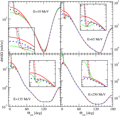
Figure 1: (color online) The convergence in the cut-off radius R of the pd elastic scattering cross section $\frac{d\sigma}{d\Omega}$ shown as a function of the c.m. angle $\Theta_{cm}$ at the incoming lab. proton energy $E=10,65,135,$ and $250$ MeV. These cross sections were calculated using approach based on Eq. (25), taking elastic scattering transition amplitude (36) with the screened Coulomb force and the AV18 nucleon-nucleon potential [25] restricted to the $j\leq 3$ partial waves. The screening radii are ($n=4$): $R=5$ fm (blue dotted line), $R=10$ fm (green solid line), $R=20$ fm (red long-dashed line), $R=30$ fm (maroon dotted line), $R=40$ fm (turquoise dotted line). The brown solid line corresponds to the $R=40$ fm result with the pure Coulomb term calculated according to Eq. (39). The red solid line is the nd elastic scattering cross section and the insets show the region of small angles.

In Fig. 1 we show the convergence in the screening radius $R$ of the pd elastic scattering cross section. The pd predictions of the first approach (25), using elastic scattering transition amplitude (36) and the Coulomb term $\left\langle{\Phi}^{\prime}\right|Pt_{c}^{R}P\left|{\Phi}\right\rangle$, calculated with the corresponding screening radius $R$, are compared with the nd angular distributions at the incoming proton or neutron lab. energies $E=10,65,135,$ and $250$ MeV. On the scale of the figure the pd cross sections for all screening radii $R$ are practically indistinguishable with exception of forward c.m. angles below $\approx 30^{o}$, shown in insets. At very forward angles cross sections for $R=5$ and $10$ fm clearly deviate but starting from $R=40$ fm the screening limit is achieved, with exception of $E=10$ MeV, which requires at forward angles even larger value of $R$. We checked that the same picture of approaching the screening limit is seen for all other elastic scattering spin observables (altogether 55 observables, including proton analyzing power, deuteron vector and tensor analyzing powers, spin correlation coefficients, as well as spin transfer coefficients from the nucleon or deuteron to the nucleon or deuteron). The achieved screening limit for a particular observable is equal to the prediction for that observable obtained with the limiting off-shell Coulomb amplitude of Eq. (39) (brown solid lines in Fig. 1), what is a very strong test of reaching the screening limit.

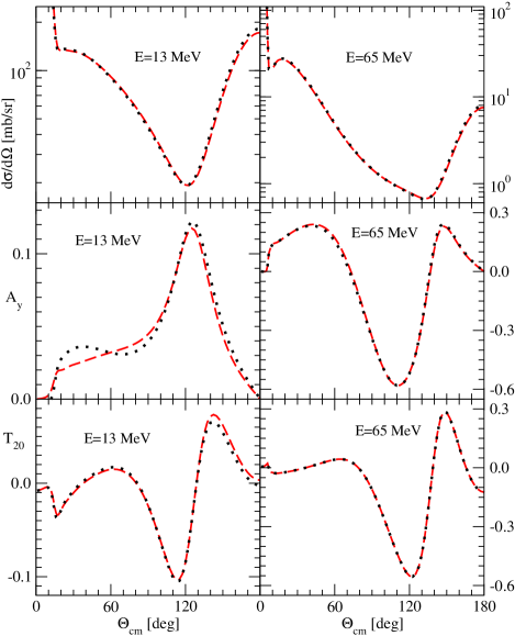
Figure 2: (color online) The predictions for the pd elastic scattering cross section $\frac{d\sigma}{d\Omega}$, proton analyzing power $A_{y}$, and for the deuteron tensor analyzing power $T_{20}$, shown as a function of the c.m. angle $\Theta_{cm}$ at the incoming lab. proton energy $E=13$ and $65$ MeV. The black dotted lines show results of the approach based on Eq. (25) and the red dashed lines on Eq. (28). In both cases the elastic scattering transition amplitude (36) was used. These observables were calculated with the screened Coulomb force ($R=40$ fm, $n=4$) and the AV18 nucleon-nucleon potential [25] restricted to the $j\leq 3$ partial waves.

At $E=13$ and $65$ MeV we compared results of the approaches based on Eqs. (25) and (28), taking the limiting screening value of $R=40$ fm. In Fig. 2 the predictions for the cross section, proton analyzing power $A_{y}$, and the deuteron tensor analyzing power $T_{20}$, of the first (Eq. (25) - the black dotted line) and second (Eq. (28) - the red dashed line) approach are shown. There is a nice agreement between predictions of both approaches at $E=65$ MeV, which extends also to other, not shown, observables. At $E=13$ MeV for some spin observables, like $A_{y}$ shown in Fig. 2, differences appear, but generally also here the agreement is good. These results demonstrate that even with such a rather small $j\leq 3$ basis cancellation effects cause that our simplified approach works quite well.

The basic difference between these two approaches lies in the treatment of the first pair of contributing Coulomb terms. While the first approach relies solely on the cancellation of contributions of these terms, in the second one they are calculated explicitly. Since one expects that the magnitude of the Coulomb terms as well as of the Coulomb force effects diminishes with increasing energy, the above mentioned differences at $13$ MeV could be interpreted as a warning that one should avoid a direct calculation of complicated terms containing 3-dimensional Coulomb t-matrix and, instead, rely on the cancellation between contributing Coulomb terms. Presently the terms with 3-dimensional Coulomb t-matrix can be calculated only for very restricted sets of partial wave states $\left|{\alpha}\right\rangle$ and total 3N angular momenta $J$, highly insufficient in full-fledged calculations needed for analyses of data.

In the following we concentrate on the first approach showing how its precision can be improved and performance controlled. It is evident that increasing the number of partial wave states $\left|{\alpha}\right\rangle$ would strengthen the cancellation effect between contributing Coulomb terms, improving thus approximation (25). Namely, for any particular value of the screening radius $R$ there is a finite number of partial wave states which reproduce exactly the 3-dimensional Coulomb t-matrix. In the extreme case when $\left|{\alpha}\right\rangle$ is taken as such a set of states, the Coulomb terms in the Faddeev equation (23) cancel exactly and the approach based on (25) becomes an exact one. Otherwise it is only an approximation, quality of which depends on how large is the cancellation effect between Coulomb terms. Since that cancellation concerns not only Coulomb terms in Eq. (25) but also to some extent in elastic scattering and breakup transition amplitudes of Eq. (33) ( (36) ), the condition reflecting degree of cancellation can be made quantitative by comparing cross sections (observables) obtained with only the first term and with all terms in (33) ( (36) ). In the case of a complete cancellation they should be equal. However, in many cases it will be sufficient when these two results converge with an increasing basis $\left|{\alpha}\right\rangle$ even to different values. Starting from an initial set of $\left|{\alpha}\right\rangle$-states one needs to extend it by incorporating consecutive states from $\left|{\beta}\right\rangle$.

To study this in more detail we extended the set of $\left|{\alpha}\right\rangle$-states by adding to the initially chosen states with $j\leq j_{s}=3$, in which both strong interactions and pp Coulomb force act, some partial wave states from set $\left|{\beta}\right\rangle$ with $j_{s}\leq j\leq j_{max}$, in which only pp Coulomb force operates. In the following such an extended set of $\left|{\alpha}\right\rangle$-states will be denoted by “$jsj_{s}jj_{max}$”, so that the initially used set is denoted by $js3j3$. We solved Eq. (25) at $E=10$ MeV for a number of extended $\left|{\alpha}\right\rangle$ sets: $js3j5,js3j7,js3j8,js3j9$, and $js3j10$, and looked for a pattern of convergence for different elastic scattering observables with a growing number of $j_{max}$. The increase in number of treated partial waves for given total angular momentum $J$ and parity $\pi$ of the $ppn$ system is large and amounts to $89$ for $js3j3$, $165$ for $js3j5$, and $539$ for $js3j10$. In spite of that increase the time required to solve numerically Faddeev equations remains restricted due to the fact that partial waves of pure Coulomb nature $\left|{\beta}\right\rangle$ (with $j_{s}\leq j\leq j_{max}$) do not couple between themselves (see a remark about the third term after (17) and Eq. (2) in Ref. [9]).

We found for practically all elastic scattering observables that the convergence in $j_{max}$ is rapid. The most influenced by changes of $j_{max}$ are low energy proton and deuteron vector analyzing powers, $A_{y}$ and $iT_{11}$, which require for converged result at $10$ MeV the basis $js3j7$. At $65$ MeV and higher energies it is sufficient to use the basis $js3j3$, what reflects the diminishing pp Coulomb force effects for higher energies.

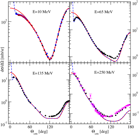
Figure 3: Comparison of data and predictions for the pd elastic scattering cross section $\frac{d\sigma}{d\Omega}$ obtained in the approach based on Eq. (25) and using elastic scattering transition amplitude (36), at the incoming proton lab. energy $E=10,65,135,$ and $250$ MeV. The cross sections were calculated with the screened Coulomb force ($R=40$ fm, $n=4$) and the AV18 nucleon-nucleon potential [25] restricted to the $j\leq 3$ partial waves. The pure Coulomb term $\left\langle{\Phi^{\prime}}|Pt_{c}P|{\Phi}\right\rangle$ was determined according to Eq. (39) (blue dashed line). At $E=10$ MeV the set $js3j7$ of $\left|{\alpha}\right\rangle$-states was used while for other energies the set $js3j3$. The red solid line is the corresponding nd elastic scattering cross section. The black circles, blue squares and red diamonds at $E=10$ MeV are pd elastic scattering cross section data of Ref. [30],  [31], and  [32], respectively. The black circles at $E=65$ MeV are pd data from  [33], at $E=135$ MeV from  [34], and at $E=250$ MeV from  [35]. The magenta squares at $E=250$ MeV are nd data from  [36].

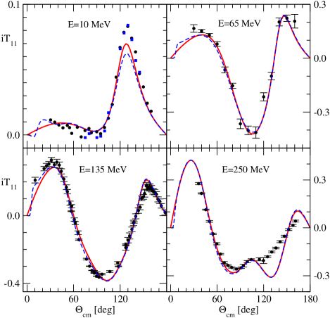
Figure 4: (color online) The same as in Fig. 3 but for the deuteron vector analyzing power $iT_{11}$. For the description of lines see Fig. 3. The black circles are pd data from  [37] at $E=10$ MeV,  [38] at $E=65$ MeV,  [39] at $E=135$ MeV, and  [40] at $E=250$ MeV. The blue squares at $E=10$ MeV are pd data from  [41].

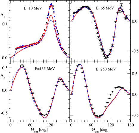
Figure 5: (color online) The same as in Fig. 3 but for the proton analyzing power $A_{y}$. For the description of lines see Fig. 3. The black circles are pd data from  [37] at $E=10$ MeV,  [33] at $E=65$ MeV,  [42] at $E=135$ MeV, and  [35] at $E=250$ MeV. The blue squares at $E=10$ MeV are pd data from  [31] and red diamonds from  [32].

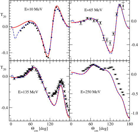
Figure 6: (color online) The same as in Fig. 3 but for the deuteron tensor analyzing power $T_{20}$. For the description of lines see Fig. 3. The black circles are pd data from  [41] at $E=10$ MeV,  [38] at $E=65$ MeV,  [39] at $E=135$ MeV, and  [40] at $E=250$ MeV.

In Figs. 3-6 we compare at different energies pd predictions of the first approach and using elastic scattering amplitude (33) containing only the first pair of Coulomb terms (taking the limiting screening value of $R=40$ fm and calculating the Coulomb term $\left\langle{\Phi}^{\prime}\right|Pt_{c}^{R}P\left|{\Phi}\right\rangle$ with the limiting off-shell Coulomb t-matrix of Eq. (39)), to available pd data for the elastic scattering cross section (Fig. 3), the deuteron vector analyzing power $iT_{11}$ (Fig. 4), the proton analyzing power $A_{y}$ (Fig. 5), and the deuteron tensor analyzing power $T_{20}$ (Fig. 6). To emphasise the importance and magnitude of Coulomb effects we provide also nd predictions for these observables. Large pp Coulomb force effects for elastic scattering observables are concentrated mainly at forward angles below $\theta_{c.m.}\approx 30^{o}$ and they diminish with an increasing energy. For the cross section the characteristic pattern caused by the pp Coulomb force is properly reproduced by the calculations. Also the forward angle data for $A_{y}$, $iT_{11}$, and $T_{20}$ are nicely reproduced. It follows that large discrepancies between pd cross section data and predictions at middle and backward c.m. angles, which grow with the increasing energy, are not caused by the pp Coulomb force and must be explained either by the action of three-nucleon forces (3NF’s) ($E=65$ and $135$ MeV)  [26] or through activation of mesonic degrees of freedom ($E=250$ MeV)  [27].

The above results were obtained omitting completely the second pair of Coulomb terms, namely the third and fifth term, in the elastic scattering transition amplitude (33). To answer the question, how are the elastic scattering observables affected by approximation (36) for the scattering amplitude, numerical calculation of both neglected terms are required. The computation of the first term in the second pair

$$-\left\langle{\vec{p}\vec{q}~{}}\right|\sum\limits_{\alpha^{\prime}}{\int{p^{\prime 2}dp^{\prime}q^{\prime 2}dq^{\prime}\left|{p^{\prime}q^{\prime}\alpha^{\prime}}\right\rangle\left\langle{p^{\prime}q^{\prime}\alpha^{\prime}}\right|}}t_{c}^{R}PG_{0}\sum\limits_{\alpha^{\prime\prime}}{\int{p^{\prime\prime 2}dp^{\prime\prime}q^{\prime\prime 2}dq^{\prime\prime}\left|{p^{\prime\prime}q^{\prime\prime}\alpha^{\prime\prime}}\right\rangle\left\langle{p^{\prime\prime}q^{\prime\prime}\alpha^{\prime\prime}}\right|}}T\left|{\Phi}\right\rangle$$

is straightforward but determination of the second one

$$\left\langle{\vec{p}\vec{q}~{}}\right|t_{c}^{R}PG_{0}\sum\limits_{\alpha^{\prime}}{\int{p^{\prime 2}dp^{\prime}q^{\prime 2}dq^{\prime}\left|{p^{\prime}q^{\prime}\alpha^{\prime}}\right\rangle\left\langle{p^{\prime}q^{\prime}\alpha^{\prime}}\right|}}T\left|{\Phi}\right\rangle,$$

which contains the 3-dimensional Coulomb t-matrix $t_{c}^{R}$, presents quite a formidable numerical task according to expression (D.9), (D.6), and (D.8) of Ref. [11]. We postpone direct numerical calculation of this term till a future study and here we would like to present some plausible arguments which justify omission of both terms in (33). To that end we investigated changes of elastic scattering observables induced by inclusion of the first term in the calculation of observables at our four energies with $js3j3$ set $\left|{\alpha}\right\rangle$. It turned out that at $E=65,135$, and $250$ MeV, the modifications are practically negligible for all $55$ elastic scattering observables. At the lowest investigated energy $E=10$ MeV, some spin observables were modified by $\approx 5-10~{}\%$. Changing the set $js3j3$ to $js3j7$ led to the similar picture at $10$ MeV. It permits us to conclude that the magnitude of the first term diminishes with the increasing energy and at the higher energies this term can be safely dropped. At the low energies its contribution is not overwhelmingly large. That together with the fact that also in elastic scattering amplitude (33) one expects a cancellation between contributions from the second pair of the Coulomb terms similar to that for the first pair, seems to justify the omission of the two terms discussed.

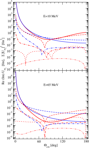
Figure 7: (color online) Comparison of the extended deuteron $\left\langle{\Phi^{\prime}}|Pt_{c}P|{\Phi}\right\rangle$ (Eq. (39)) and the point deuteron $A_{c}$ [29] pd scattering Coulomb amplitudes. The red and blue solid lines are sums, over all incoming and outgoing proton and deuteron spin projections, of the squares of the extended and point deuteron amplitudes, respectively. The blue short dashed and dashed-dotted lines (the red short-dashed and dashed-dotted) are absolute values of real (imaginary) parts of the point and extended deuteron amplitudes, respectively, for transition from the incoming proton ($-\frac{1}{2}$) and deuteron ($-1$) spin projections to the outgoing ($-\frac{1}{2}$) and ($-1$) ones. The red dotted and red dashed-double-dotted lines are absolute values of real and imaginary parts of the extended deuteron amplitude, respectively, for nondiagonal transition from the incoming proton ($-\frac{1}{2}$) and deuteron ($0$) spin projections to the outgoing ($-\frac{1}{2}$) and ($-1$) ones.

Last but not least, in Fig. 7 we compare at two lab. energies of the incoming proton $E=10$ and $65$ MeV the point deuteron pd Coulomb amplitude $A_{c}$  [29] with the extended deuteron one, $\left\langle{\Phi}|Pt_{c}R|{\Phi}\right\rangle$, calculated with the limiting Coulomb t-matrix of Eq. (39). While the $A_{c}$ is diagonal in incoming and outgoing proton and deuteron spin projections, the extended deuteron amplitude permits also nondiagonal terms, which however are few orders of magnitude smaller than the diagonal ones. The red and blue solid lines are sums, over all incoming and outgoing proton and deuteron spin projections, of the squares of the extended and point deuteron amplitudes, respectively. There is a nice agreement between both amplitudes in the most important region of angles up to $\approx 30^{o}$, not only for that sum but also for the magnitudes of their real parts. The imaginary parts are much more smaller. It is illustrated in Fig 7 for the case of a transition from $m_{d}^{in}=-1,m_{p}^{in}=-\frac{1}{2}$ to $m_{d}^{out}=-1,m_{p}^{out}=-\frac{1}{2}$. Also the non diagonal term for the extended deuteron, for transition from $m_{d}^{in}=0,m_{p}^{in}=-\frac{1}{2}$ to $m_{d}^{out}=-1,m_{p}^{out}=-\frac{1}{2}$, is shown.

III.2 Breakup reaction

The exclusive breakup reaction offers a rich spectrum of kinematically complete geometries with observables sensitive to underlying dynamics. We decided to focus on three geometries specified by a kinematical condition for momenta of the three outgoing nucleons. In the so called final-state-interaction (FSI) geometry the two outgoing nucleons have equal momenta. In neutron-deuteron (nd) breakup their strong interaction in the ${}^{1}S_{0}$ state leads to a characteristic cross section maximum occurring at the exact FSI condition, the magnitude of which is sensitive to the ${}^{1}S_{0}$ scattering length. In the symmetrical-space-star (SST) configuration the momenta of the three outgoing nucleons in the 3N center-of-mass (c.m.) have the same magnitudes and form a three-pointed ”Mercedes-Benz” star. That star lies in a plane inclined under an angle $\alpha$ with respect to the beam direction with momenta of the two outgoing and detected nucleons (in our case protons) lying symmetrically to the beam. The quasi-free-scattering (QFS) geometry refers to a situation where one of the nucleons is at rest in the laboratory system. In pd breakup the np or pp QFS configurations are possible, while for nd breakup np or neutron-neutron (nn) quasi-freely scattered pairs can emerge.

The characteristic feature of the exact approach of Refs.  [11] and  [12] as well as of our simplified one is the appearance in the breakup transition amplitude of a new term, $\left\langle\vec{p}_{0}\vec{q}\right|(1+P)t_{c}^{R}P\left|{\Phi}\right\rangle$, based on a 3-dimensional Coulomb t-matrix, $t_{c}^{R}$, analogous to the Rurherford term in the elastic pd scattering. The expression for this term given in Appendix C of Ref. [11] (Eq. (C.3)) shows that largest contributions from this term are expected in the region of the breakup phase space where the argument of the deuteron wave function, ${\varphi_{L}(|\vec{q}+\frac{1}{2}\vec{q}_{0}|)}$, vanishes. That condition $\vec{q}=-\frac{1}{2}\vec{q}_{0}$ occurs in the pp QFS, where the spectator neutron rests in the laboratory system (see also the discussion on p.185 of Ref. [5]). Therefore one expects large pp Coulomb force effects for that geometry. Also large Coulomb effects are expected in the pp FSI region, where two outgoing protons have equal momenta and interact strongly. For nn FSI this leads to a pronounced cross section maximum just at the nn FSI condition and in the case of pp FSI the Coulomb barrier should prevent such a maximum from forming.

In the following we start to investigate the breakup reaction using approach (25) with the set $js3j3$ and the breakup transition amplitude of Eq. (36). First we demonstrate the pattern of convergence to the screening limit in two exclusive geometries, QFS as well as FSI, and show that the final results do not depend on how specifically the on-shell breakup amplitudes, which undergo renormalization, are derived. We will apply renormalization to the on-shell breakup amplitudes obtained in two different ways. In the first approach the on-shell breakup amplitudes $\left\langle p_{0}q\alpha\right|T^{R}\left|{\Phi}\right\rangle$ ($\left\langle p_{0}q\alpha\right|t_{c}^{R}P\left|{\Phi}\right\rangle$) are obtained by interpolation from the off-shell ones $\left\langle pq\alpha\right|T^{R}\left|{\Phi}\right\rangle$ ($\left\langle pq\alpha\right|t_{c}^{R}P\left|{\Phi}\right\rangle$), with subsequent removal of the oscillating phase factor $e^{i\Phi^{R}_{n}}$ when calculating the breakup transition amplitude. In the second method we generate the half-shell pp t-matrix $t_{N+c}^{R}(p_{0},p^{\prime};E-\frac{3}{4m}q^{2})$ ($t_{c}^{R}(p_{0},p^{\prime};E-\frac{3}{4m}q^{2})$) and calculate the on-shell transition matrix elements $\left\langle p_{0}q\alpha\right|T^{R}\left|{\Phi}\right\rangle$ ($\left\langle p_{0}q\alpha\right|t_{c}^{R}P\left|{\Phi}\right\rangle$) according to Eq. (48). Here one has to use unrenormalized $t_{N+c}^{R}(p_{0},p^{\prime};E-\frac{3}{4m}q^{2})$ ($t_{c}^{R}(p_{0},p^{\prime};E-\frac{3}{4m}q^{2})$) and postpone again the renormalization to calculation of the breakup transition amplitude.

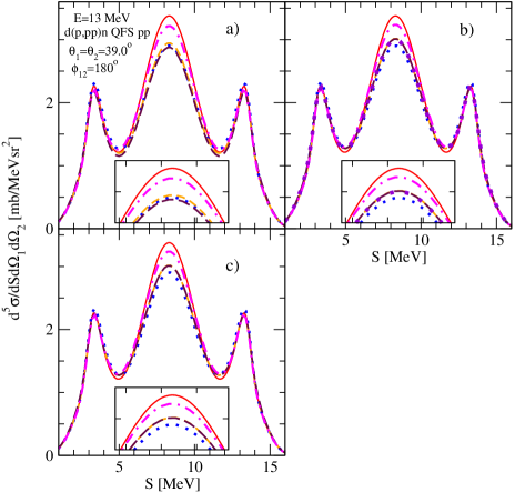
Figure 8: (color online) The convergence with respect to the cut-off radius R of the pd breakup cross section $\frac{d^{5}\sigma}{d\Omega_{1}d\Omega_{2}dS}$ shown as a function of the S-curve length for the pp QFS kinematically complete configuration at the incoming proton lab. energy $E=13$ MeV. The screening radii are ($n=4$): $R=5$ fm (blue dotted line), $R=10$ fm (magenta dashed-dotted line), $R=20$ fm (orange short-dashed line), $R=40$ fm (maroon long-dashed line). These cross sections were calculated using the approach based on Eq. (25) with the screened Coulomb force and the AV18 nucleon-nucleon potential [25] restricted to the $j\leq 3$ partial waves (set $js3j3$), taking the on-shell Faddeev amplitudes obtained in two different ways and applying renormalization when calculating the breakup transition amplitude. In a) unrenormalized on-shell amplitudes gained by interpolation from the off-shell ones were used. In b) the on-shell amplitudes of a) have been renormalized before calculating observables. In c) the on-shell amplitudes were calculated according to (48) with the unrenormalized pp part of $t_{N+c}^{R}$ ($t_{c}^{R}$) and renormalization was performed before calculating observables. The red solid line is the corresponding nd elastic scattering cross section. The violet dotted line in b) is the result with $R=40$ fm but the pure Coulomb term $\left\langle{\vec{p}_{0}\vec{q}}|(1+P)t_{c}P|{\Phi}\right\rangle$ determined with the $t_{c}$ of Eq. (55).

In Fig. 8 we present the pattern of convergence in the screening radius $R$ for the pp QFS. Taking unrenormalized on-shell breakup amplitudes obtained by an interpolation from the off-shell solutions of the Faddeev equations to the on-shell values $(p_{0},q)$ provides unrenormalized pp QFS cross sections which change with varying $R$ (Fig. 8a). Renormalizing these amplitudes stabilizes the cross sections for the screening radii $R\geq 20$ fm (see Fig. 8b). The limiting values of the pp QFS cross sections do not depend on the way the on-shell breakup amplitudes are determined (see Figs. 8b and 8c). These two methods lead to the same final pp QFS cross sections. That the screening limit has been achieved is confirmed in Fig. 8b, where the violet dotted line shows the result for $R=40$ fm with the pure Coulomb term $\left\langle{\vec{p}_{0}\vec{q}}|(1+P)t_{c}P|{\Phi}\right\rangle$ determined using the final 3-dimensional Coulomb t-matrix of Eq. (55).

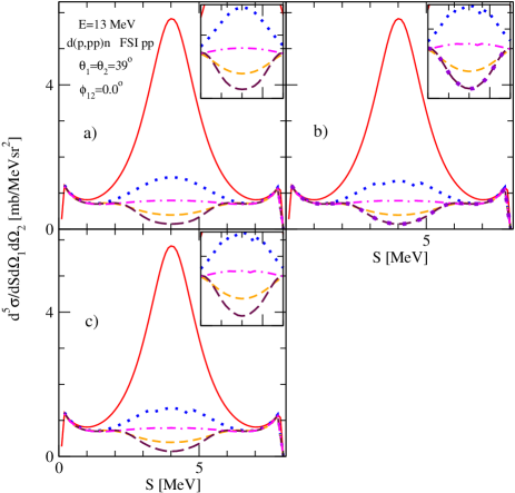
Figure 9: (color online) The same as in Fig. 8 but for the pp FSI kinematically complete configuration.

In Fig. 9 we present analogous investigation for the pp FSI configuration. The large effect of the pp Coulomb force is seen in the region of FSI, where, instead of a clear maximum present for nn FSI, the cross section is reduced practically to zero by the pp Coulomb barrier. The pattern of approaching the limiting value is similar as in the case of the pp QFS and final result also here does not depend on how the on-shell breakup amplitudes were derived. To get the final values of the cross section one needs to go to a larger screening radius than in the case of the pp QFS (see Fig.9b).

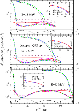
Figure 10: (color online) The pd breakup d(p,pp)n cross section calculated at the pp QFS condition for the incoming proton lab. energy $E=13,19,$ and $65$ MeV, as a function of the angle of the outgoing proton 1. The approach based on Eq. (25) with set of $js3j3$ partial waves and the screening radius $R=40$ fm ($n=4$) was used, with on-shell Faddeev amplitudes obtained by an interpolation from the off-shell ones, renormalized before calculating observables. The blue long-dashed line is the result with all three terms in Eq. (36). Also the result without renormalization is shown by the green dotted line. The maroon dotted and magenta dashed-dotted lines follow when the term with 3-dimensional $t_{c}^{R}$ Coulomb t-matrix and both terms with $t_{c}^{R}$ are omitted, respectively, and the black double-dotted-dashed line when only these two terms are kept. At bottom of each figure continuation of the black double-dotted-dashed line is shown in a compressed y-axis scale shown on the right side. The red solid line is the nd breakup cross section. In insets the lab. cross sections $d\sigma/d\Omega$ ($\frac{mb}{sr}$) for pp scattering at lab. energies $E=10,20,$ and $65$ MeV are shown as a function of the proton lab. angle. Here the red solid and blue dashed lines are the AV18 cross sections without and with pp Coulomb interaction, respectively.

In Fig. 8 non-negligible effects of renormalization (Fig. 8a and b), which raise the cross section by $\approx 5\%$ in the maximum, are seen for that particular pp QFS configuration. In order to investigate the renormalization as well as the pp Coulomb force effects for all pp QFS configurations, we looked at the pp quasi-free-scattering cross section exactly at the QFS condition (maximum of the cross section) as a function of the lab. angle of the first outgoing proton $\theta_{1}^{lab}$ ($d(p,p_{1}p_{2})n$). Since later we will compare theoretical predictions to available pp QFS cross section data at $E=9.5,13,19,22.7,$ and $65$ MeV, we show in Fig. 10 results of this investigation for three energies: $E=13,19,$ and $65$ MeV. At each energy at given $\theta_{1}^{lab}$ there are 2 solutions for the QFS condition, the second one (upper branch in Fig. 10) being not (or difficult) accessible to measurement due to too small energy of one of the outgoing protons. The full result with renormalization is given by the blue long-dashed line which compared with the green dotted line (without renormalization) reveals importance and the magnitude of renormalization. The non-negligible renormalization effects at $E=13$ MeV of the order of $\approx 5-8\%$ are seen only for $\theta_{1}^{lab}\in(10^{o},50^{o})$. At $19$ and $65$ MeV the renormalization causes in pp QFS only insignificant effects.

In order to get the information of the Coulomb force effects in Fig. 10 also the nd prediction is shown by the solid red line. The Coulomb effects are largest at $E=13$ MeV as evidenced by the nd results as well as by the maroon dotted line, resulting when the term with the 3-dimensional Coulomb t-matrix is omitted, or by magenta dashed-dotted line, when both Coulomb terms are absent. They diminish rapidly with growing energy, becoming practically negligible at $65$ MeV. It is interesting to note that the angular dependence of the pp QFS cross section resembles that of pd elastic scattering, with the characteristic increase at forward angles caused by the Coulomb term $\left\langle\vec{p}_{0}\vec{q}\right|(1+P)t_{c}^{R}P\left|{\Phi}\right\rangle$. Also the importance and magnitude of the Coulomb force effects in pp QFS resembles those in a free pp scattering (see insets in Fig. 10). To exemplify the cancellation effect between the first pair of Coulomb terms in the pp QFS breakup transition amplitude we show in Fig. 10 also cross sections (black double-dotted-dashed line) obtained with these two terms only. In the region of angles $\theta_{1}^{lab}\in(10^{o},40^{o})$ the resulting values of that cross section are about $\approx 10^{-1}\frac{mb}{MeV*sr^{2}}$ for that set of $|\alpha>$-states, what illustrates quite significant cancellation, however not so large as for the case of the pp FSI or pd SST (see below).

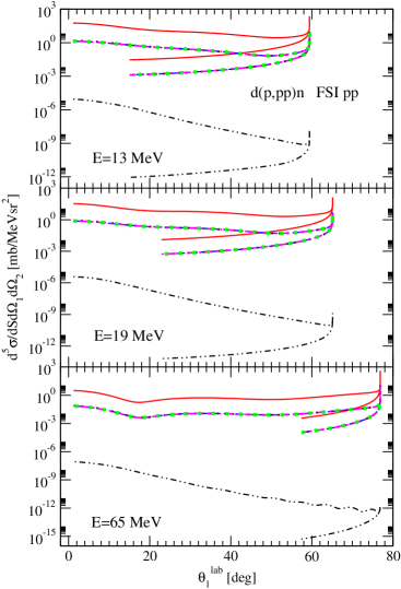
Figure 11: (color online) The same as in Fig. 10 but for the pd breakup d(p,pp)n cross section $d^{5}\sigma/d\Omega_{1}d\Omega_{2}dS$ calculated at the pp FSI condition ($\vec{p}_{1}=\vec{p}_{2}$).

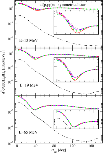
Figure 12: (color online) The same as in Fig. 10 but for the pd breakup d(p,pp)n cross section $d^{5}\sigma/d\Omega_{1}d\Omega_{2}dS$ calculated at the symmetrical-space-star condition (in the 3N c.m. system the momenta of the three outgoing nucleons are equal and form a symmetric three-point star in a plane inclined at an angle $\alpha_{cm}$ with respect to the incoming proton momentum).

In Figs. 11 and 12 results of a similar investigation are shown for pp FSI and pd SST, respectively. The action of the Coulomb barrier brings the pp FSI cross section close to zero for all pp FSI configurations. Regardless from their production angle $\theta_{1}^{lab}$, the renormalization effect is insignificant and the cancellation between two contributing Coulomb terms appears drastic (black double-dotted-dashed line). The pp FSI cross section is determined practically by only the first term in the breakup transition amplitude (36). For the SST configurations the largest effects of renormalization as well as of the pp Coulomb force are present at $E=13$ and $19$ MeV around $\alpha_{cm}\approx 40^{o}$. They become again negligible at $E=65$ MeV. When the star plane is perpendicular to the beam direction the renormalization effects are small. As for the pp FSI, the cancellation effects in the breakup transition amplitude for that configuration are very large.

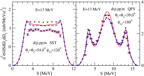
Figure 13: (color online) The pd complete breakup d(p,pp)n cross sections $d^{5}\sigma/d\Omega_{1}d\Omega_{2}dS$ for the SST and pp QFS configurations at $13$ MeV of the incoming proton lab. energy as a function of the arc-length of the S-curve. They are obtained with the screening radius $R=40$ fm ($n=4$) and set $js3j3$ partial waves, using approach based on Eq. (25) (blue short-dashed line) or (28) (maroon dotted line). In both approaches the 3-dimensional Coulomb t-matrix is determined according to (55). The on-shell Faddeev amplitudes obtained by interpolation from the off-shell ones are used and renormalized before calculating observables. The red solid line is the corresponding nd breakup cross section. The maroon circles are pd data from Ref. [43].

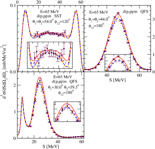
Figure 14: The same as in Fig. 13 but for the pd complete breakup d(p,pp)n cross sections $d^{5}\sigma/d\Omega_{1}d\Omega_{2}dS$ in SST and pp QFS at $65$ MeV. Here in both approaches the 3-dimensional Coulomb t-matrix was determined by solving the 3-dimensional Lippmann-Schwinger equation with the screening radius $R=40$ fm ($n=4$). In case of the approach based on Eq. (25) effects of using 3-dimensional Coulomb t-matrix determined according to (55) is shown by the orange dotted lines. The maroon circles are pd data from Ref. [44].

In Figs. 13 and 14 we show examples of comparison of our theoretical predictions to pd breakup cross section data at $E=13$ and $65$ MeV for SST ($\alpha_{cm}=90^{o}$) and pp QFS configurations. We show predictions of our two approaches, one based on Eq. (25) (blue short-dashed line) and second on Eq. (28) (maroon dotted line). At $13$ MeV they agree very well with each other for pp QFS, differing by $\approx 10\%$ for SST. Both disagree significantly with the pd SST cross section data, underestimating slightly pp QFS data. At $65$ MeV they are close to each other and agree quite well with the SST data, differing again only slightly from the pp QFS data. This is similar to what we have found for elastic scattering when comparing these two approaches and seems to support the validity of the assumption about the cancellation of the Coulomb terms in the first approach, at the same time indicating that using directly computed complex terms with 3-dimensional Coulomb t-matrix is hazardous.

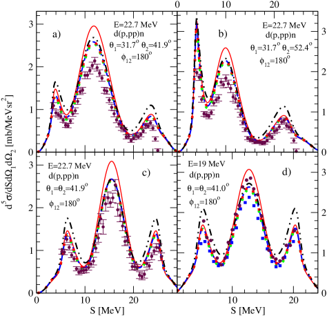
Figure 15: (color online) The pd complete breakup d(p,pp)n cross sections $d^{5}\sigma/d\Omega_{1}d\Omega_{2}dS$ for pp QFS configurations at $22.7$ MeV ( a), b), and c) ) and $19$ MeV ( d) ) of the incoming proton lab. energy, as a function of the arc-length of the S-curve. They were obtained with the screening radius $R=40$ fm ($n=4$) using approach based on Eq. (25) and set $js3j3$ of partial waves. The on-shell Faddeev amplitudes obtained by interpolation from the off-shell ones were used and renormalized before calculating observables with amplitude of Eq. (36) (blue short-dashed line). The green dotted line is a result without renormalization. The black double-dotted-dashed line shows the result when also the third term in (33) is included in the breakup transition amplitude. The red dotted line is obtained with the limiting $t_{c}$ of Eq. (55). The red solid line is the corresponding nd breakup cross section. The maroon circles are pd data from Ref. [45] for a), b), and c), and from Ref. [46] for d). The blue squares in d) are pd data from Ref. [46].

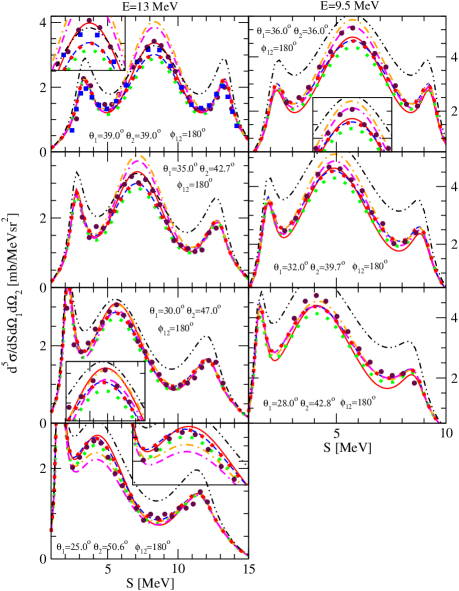
Figure 16: (color online) The same as in Fig. 15 but for the pp QFS configurations at $13$ MeV and $9.5$ MeV. The orange dashed-dotted and magenta double-dashed-dotted lines are renormalized and unrenormalized results, respectively, when both Coulomb terms are omitted in the breakup transition amplitude (36). The red solid line is the nd breakup cross section. The maroon circles are pd data from Ref. [47] and blue squares at $13$ MeV are pd data from Ref. [31].

In Ref. [47] a correct description of the low energy pp QFS cross section data was reported. That prompted us to reanalyze available low energy pp QFS cross section data and look for a possible reason of the slight discrepancy found at $13$ MeV in Fig. 13. In Fig. 15 we compare $E=19$ MeV data of Ref. [46] and $E=22.7$ MeV data of Ref. [45] to our theoretical predictions obtained with the renormalized and unrenormalized $js3j3$ on-shell breakup amplitudes of Eq.(36), received by interpolation from the off-shell ones (blue short-dashed and green dotted lines, respectively). The same comparison at $E=9.5$ and $13$ MeV for the data from Ref. [47] and at $13$ MeV for the data from Ref. [43], is presented in Fig. 16. To make sure that the screening limit have been achieved we show in both figures by the red dotted lines also the renormalized $R=40$ fm results obtained with the pure Coulomb term calculated according to (55).

A glance at both figures reveals again that the renormalization effects shrink with the growing energy. While at $9.5$ and $13$ MeV they are non-negligible and enhance the cross section bringing the theory closer to the data, at $19$ and $22.7$ MeV they are practically insignificant. It is interesting to notice that large effects of the pp Coulomb force at smaller energies have a pattern of contributions changing with pp QFS configuration (see the orange dashed-dotted and magenta double-dashed-dotted lines in Fig. 16, which show the results when both Coulomb terms are omitted). At $9.5$ and $13$ MeV theory slightly underestimates pp QFS cross sections in practically all configurations. At $19$ MeV theory lies between two available data sets and at $22.7$ MeV the data are clearly overestimated.

The contribution to a particular kinematically complete breakup configuration, specified by momenta of three outgoing nucleons, comes from only three sets $(p_{i},q_{i})$ of Jacobi-relative-momenta values, belonging to an ellipse of Eq. (40) in a $q-p$ plane. Performing exclusive breakup measurements one is restricted only to points from that curve, what makes the exclusive breakup reaction a very selective tool. In contrast to the breakup reaction, averaging over the relative momentum of nucleons forming the deuteron causes, that elastic pd scattering gets contributions from a large region in the $q-p$ plane, which does not overlap with the elliptic curve for the breakup reaction (see Fig. 1 in [28]). It follows that breakup observables should reveal greater sensitivity to the underlying dynamics than elastic pd scattering observables. This motivated us to investigate how the extension of the set $\left|{\alpha}\right\rangle$, which has only a small effect on elastic scattering observables, influences the pp QFS cross sections.

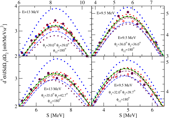
Figure 17: (color online) The pattern of convergence in the sets of partial waves around the QFS pp condition for cross sections in chosen configurations from Fig.16, calculated with the amplitude of Eq. (36). The meaning of the data symbols is the same as in Fig. 16. Equally colored dashed and dotted lines correspond to identical set of partial waves. For dashed lines all three terms in Eq. (36) contribute to the breakup amplitude while for dotted lines only the first term in (36) was taken into account. The sets of partial waves are: blue - $js3j3$, maroon - $js3j5$, red - $js3j7$. For the set $js3j8$ the color of lines are solid green and black dotted for the case when all three and only the first term were taken into account, respectively. The red circles show the cross sections calculated with the set js3j8 and all five terms of Eq. (33) included in the breakup amplitude.

In Fig.17 we show the pattern of convergence in partial wave expansion of the pp QFS cross section around QFS point for some pp QFS configurations from Fig.16. The differently colored dashed lines as well as the solid green line are cross sections based on solutions of the Faddeev equation (25) with different partial wave sets and transition amplitude containing all three terms in Eq. (36). The dotted lines show the cross sections resulting when only the first term in (36) was kept and the two Coulomb terms were omitted. The same colored lines correspond to the same set of $\left|{\alpha}\right\rangle$-states, with the exception of black dotted and solid green lines, which correspond to $js3j8$ set. Starting from the set $js3j3$, for which large effect of omitting the Coulomb terms is seen and separation between blue dotted and dashed lines is large, the difference between dashed and dotted lines diminishes rapidly with increasing $j$ and disappears for $js3j8$ set. Also the dashed lines themselves are converging to the prediction obtained for the set $js3j8$. Including additional partial waves with $j=9$ and higher does not change the results. It is clear that extending set $\left|{\alpha}\right\rangle$ improves the description of data. That points not only to the need for treatment of higher partial waves in breakup but the convergence of dotted and dashed results supports also our expectation about the stronger cancellation between contributing Coulomb terms with the increasing number of partial waves.

Last but not least we investigate the significance of additional two Coulomb contributions to the breakup amplitude of Eq. (33) (the third and fifth terms) omitted up to now, namely the terms

$$-\left\langle{\vec{p}\vec{q}~{}}\right|\sum\limits_{\alpha^{\prime}}{\int{p^{\prime 2}dp^{\prime}q^{\prime 2}dq^{\prime}\left|{p^{\prime}q^{\prime}\alpha^{\prime}}\right\rangle\left\langle{p^{\prime}q^{\prime}\alpha^{\prime}}\right|}}t_{c}^{R}PG_{0}\sum\limits_{\alpha^{\prime\prime}}{\int{p^{\prime\prime 2}dp^{\prime\prime}q^{\prime\prime 2}dq^{\prime\prime}\left|{p^{\prime\prime}q^{\prime\prime}\alpha^{\prime\prime}}\right\rangle\left\langle{p^{\prime\prime}q^{\prime\prime}\alpha^{\prime\prime}}\right|}}T\left|{\Phi}\right\rangle$$

and

$$\left\langle{\vec{p}\vec{q}~{}}\right|t_{c}^{R}PG_{0}\sum\limits_{\alpha^{\prime}}{\int{p^{\prime 2}dp^{\prime}q^{\prime 2}dq^{\prime}\left|{p^{\prime}q^{\prime}\alpha^{\prime}}\right\rangle\left\langle{p^{\prime}q^{\prime}\alpha^{\prime}}\right|}}T\left|{\Phi}\right\rangle~{}.$$

That their contribution can be important is visualised in Figs. 15 and 16, where the black double-dotted-dashed lines show the cross section obtained when in addition to three contributions in (36) also the term

$$-\left\langle{\vec{p}\vec{q}~{}}\right|\sum\limits_{\alpha^{\prime}}{\int{p^{\prime 2}dp^{\prime}q^{\prime 2}dq^{\prime}\left|{p^{\prime}q^{\prime}\alpha^{\prime}}\right\rangle\left\langle{p^{\prime}q^{\prime}\alpha^{\prime}}\right|}}t_{c}^{R}PG_{0}\sum\limits_{\alpha^{\prime\prime}}{\int{p^{\prime\prime 2}dp^{\prime\prime}q^{\prime\prime 2}dq^{\prime\prime}\left|{p^{\prime\prime}q^{\prime\prime}\alpha^{\prime\prime}}\right\rangle\left\langle{p^{\prime\prime}q^{\prime\prime}\alpha^{\prime\prime}}\right|}}T\left|{\Phi}\right\rangle$$

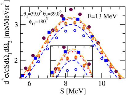
Figure 18: (color online) The pattern of convergence in the sets of partial waves around the QFS pp condition for cross section of the first configuration at $E=13$ MeV from Fig.16, calculated with the amplitude of Eq. (36) (lines) and (33) (circles). The meaning of the data symbols is the same as in Fig. 16. Equally colored lines and circles correspond to identical set of partial waves. For lines all three terms in (36) and for circles all five terms in (33) contribute to the breakup amplitude. The sets of partial waves are: blue (short-dashed) - $js3j3$, red (dotted) - $js3j5$, brown (long dashed) - $js3j7$, and orange (long dashed) - $js3j8$.

was included. The changes of the cross section are quite large at lower energies and become much smaller at $19$ and $22.7$ MeV, confirming again diminishing of the Coulomb force effects with growing energy. Since changes of the cross section induced by this term are non-negligible, it is unavoidable to include in the transition amplitude also the term $\left\langle{\vec{p}\vec{q}~{}}\right|t_{c}^{R}PG_{0}\sum\limits_{\alpha^{\prime}}{\int{p^{\prime 2}dp^{\prime}q^{\prime 2}dq^{\prime}\left|{p^{\prime}q^{\prime}\alpha^{\prime}}\right\rangle\left\langle{p^{\prime}q^{\prime}\alpha^{\prime}}\right|}}T\left|{\Phi}\right\rangle$. One would expect that, similarly as for the first pair of the two Coulomb terms in (33), also terms in the second pair would probably cancel each other when extending the set $|\alpha>$. To check it requires, however, a calculation of this nontrivial modification of the Rutherford term by the strong nucleon-nucleon interactions, as given in Appendix D of Ref.  [11] (Eqs. (D.6)-(D.8)). In Fig. 18 we show the convergence pattern in $j$ for the first pp QFS configuration at $13$ MeV, where circles represent cross sections obtained with all the five terms included in the breakup amplitude (33). To facilitate the comparison we also show again by different lines the convergence pattern with only three terms in the breakup amplitude (36). It is seen that indeed circles converge rapidly to the result which in the maximum of that pp QFS is $\approx 5\%$ smaller than prediction obtained with only the first pair of Coulomb terms in the breakup transition amplitude. It shows that the two contributions in the second pair of the Coulomb terms of the breakup transition amplitude (33) do not cancel each other completely in the QFS maximum.

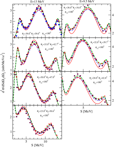
Figure 19: (color online) The pd complete breakup d(p,pp)n cross sections $d^{5}\sigma/d\Omega_{1}d\Omega_{2}dS$ for the configurations from Fig. 16, calculated using approach based on Eq. (25) and set $js3j8$ of partial waves, with on-shell Faddeev amplitudes obtained by interpolation from the off-shell ones, renormalized before calculating observables. The screening radius $R=40$ fm ($n=4$) was used and the green solid lines show the results with all three terms in (36) contributing to the breakup amplitude, while for the black dotted lines only the first term was taken into account. The red circles show the cross sections calculated with all five terms in (33) included in the breakup amplitude. For the sake of comparison also results with the set $js3j3$ and three terms in (36) contributing to the breakup amplitude, are shown (the blue short-dashed line). The red solid line is the corresponding nd cross section. The meaning of the data symbols is the same as in Fig. 16.

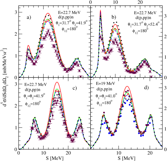
Figure 20: (color online) The same as in Fig. 19 but for the configurations from Fig. 15.

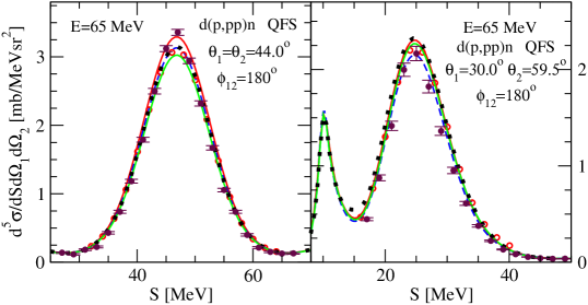
Figure 21: (color online) The same as in Fig. 19 but for the pp QFS configurations from Fig. 14.

In Figs.19, 20, and 21, we show converged results obtained with $js3j8$ set for all investigated here pp QFS configurations at $9.5$ and $13$, $19$ and $22.7$, and $65$ MeV, respectively. At $9.5$ and $13$ MeV the description of data by the three-term amplitude (36) (the green solid line)) is significantly improved when compared to $js3j3$ set predictions (the blue short-dashed line). Including in addition the second pair of the Coulomb terms lowers by $\approx 5\%$ cross sections in all the QFS maxima, deteriorating slightly the good description of data in that region, leaving it, however, without a change beyond the QFS peak region. At the higher energies the contribution from the second pair becomes insignificant and a nice agreement with data at $19$ and $65$ MeV is found. The large discrepancies to data at $22.7$ MeV remain.

IV Summary and conclusions

We formulated and applied a simplified approach to the exact treatment of the pp Coulomb force in the momentum space 3N Faddeev calculations, presented in Refs. [11] and  [12]. That exact treatment is based on a standard formulation for short range forces and relies on a screening of the long-range Coulomb interaction. It is, however, unhandy for applications since it contains two contributing terms with a 3-dimensional Coulomb t-matrix, which require an unrealistic amount of computer time and resources to compute them in practise. That prevents any application of the exact approach in full-fledged 3N calculations. Our simplified approach contains the main physical ingredients of the exact method but neglects these complex terms altogether, relying on their cancellation. We have applied it in a wide energy range of the incoming proton, using the AV18 NN potential to calculate elastic pd scattering and breakup observables. The main results are summarized as follows.

• We demonstrated and showed numerically that the elastic pd scattering amplitude has a well defined screening limit and therefore does not require any renormalization. This is an implication of the fact that only off-shell values of Jacobi momenta and consequently, only off-shell 2N t-matrices are required and enter in the determination of that amplitude. Well converged elastic pd cross sections and spin observables are obtained at finite screening radii. Additional support for the claim that infinite R limit is achieved, was provided by using directly the limiting analytical expression for the 3-dimensional off-shell Coulomb t-matrix when calculating the transition amplitude.

• Contrary to pd elastic scattering, for pd breakup it is unavoidable to perform renormalization of the breakup amplitudes. The reason is that in breakup only the amplitudes for on-shell values of Jacobi momenta are required, what demands in consequence also half-shell 2N t-matrices. The breakup amplitudes have two contributions, one driven by the interaction in the pp subsystem and second by that in the np subsystem. Only the first part requires renormalization. We demonstrated that the renormalization has to be performed during calculation of the breakup transition amplitude and the on-shell amplitudes themselves can be derived in two different ways which lead to the same results. We have shown that converged results for breakup can be achieved with finite screening radii. The importance of the renormalization depends on the energy of a 3N system and on the region in the breakup phase-space. It is diminishing with the growing energy, and remains very important at low energies, especially in the region of QFS condition.

• In our approach to breakup two new terms appear. One corresponds to the Rutherford pd Coulomb amplitude in elastic pd scattering. This term was found to be important in the region of QFS scattering. Calculating that term with the exact expression for a 3-dimensional half-on-shell Coulomb t-matrix provides an additional test that the screening limit for breakup is achieved. The second term is a correction to the first one due to strong interactions between nucleons. We found that its contribution reduces the low energy pp QFS cross sections by $\approx 5\%$ in the QFS maximum.

• We have checked the validity of the basic assumption underlying our simplified approach in the case of a restricted basis of partial wave states, for which it was possible to compute the first term with a 3-dimensional Coulomb t-matrix in the exact approach. Also results for contributions to the elastic scattering and breakup transition amplitudes, obtained with an extended basis of states, vindicate the cancellation effect between Coulomb terms. The presented results justify using our simplified approach, whose requirements for computer time and resources are comparable to standard nd calculations, in future applications. This insures that the pp Coulomb force effects for pd reactions can be calculated efficiently and quickly.

• We found that large Coulomb force effects are restricted to forward angles for the elastic pd scattering and to specific regions of the breakup phase-space. They seem generally to diminish rapidly with the increasing energy of the pd system.

The simplified approach proposed by us can be applied also in the case when in addition to pairwise forces a 3NF contributes to the 3N Hamiltonian. Since the structure of Faddeev equations is very similar an extension to 3N reactions with electromagnetic probes is straightforward.

References

• [1] E. O. Alt, W. Sandhas, and H. Ziegelmann, Phys. Rev. C 17, 1981 (1978).
• [2] E. O. Alt and W. Sandhas, in Coulomb Interactions in Nuclear and Atomic Few-Body Collisions, ed. by F.S. Levin and D. Micha (Plenum, New York 1996), p.1.
• [3] E. O. Alt and M. Rauh, Phys. Rev. C49, R2285 (1994).
• [4] E. O. Alt, A. M. Mukhamedzhanov, M. M. Nishonov, and A. I. Sattarov, Phys. Rev. C65, 064613 (2002).
• [5] W. Glöckle, H. Witała, D. Hüber, H. Kamada, J. Golak, Phys. Rep. 274, 107 (1996).
• [6] A. Kievsky, M. Viviani, and S. Rosati, Phys. Rev. C 52, R15 (1995).
• [7] A. Deltuva, A. C. Fonseca, and P. U. Sauer, Phys. Rev. C72, 054004 (2005).
• [8] A. Deltuva, A. C. Fonseca, and P. U. Sauer, Phys. Rev. C71, 054005 (2005).
• [9] A. Deltuva, A. C. Fonseca, and P. U. Sauer, Phys. Rev. C73, 057001 (2006).
• [10] E. Stephan et al., Phys. Rev. C76, 057001 (2007).
• [11] H. Witała, R. Skibiński, J. Golak, W. Glöckle, Eur. Phys. Journal A41, 369 (2009).
• [12] H. Witała, R. Skibiński, J. Golak, W. Glöckle, Eur. Phys. Journal A41, 385 (2009).
• [13] H. Witała, W. Glöckle, H.Kamada, Phys. Rev. C43, 1619 (1991).
• [14] J.C.Y. Chen and A.C. Chen, in Advances of Atomic and Molecular Physics, edited by D. R. Bates and J. Estermann ( Academic, New York, 1972), Vol. 8.
• [15] L. P. Kok, H. van Haeringen, P hys. Rev. C21, 512 (1980).
• [16] W. Glöckle, The Quantum Mechanical Few-Body Problem, Springer Verlag 1983.
• [17] W.F. Ford, Phys. Rev. 133, B1616 (1964).
• [18] W.F. Ford, J. Math. Phys. 7, 626 (1966).
• [19] M. Yamaguchi, H. Kamada, and Y. Koike, Prog. Theor. Phys. 114 , 1323 (2005).
• [20] J.R. Taylor, Nuovo Cimento B23, 313 (1974).
• [21] M.D. Semon and J.R. Taylor, Nuovo Cimento A26, 48 (1975).
• [22] M. Abramowitz, I.A. Stegun, (Editors) Handbook of Mathematical Functions, (Dover Publ., N.Y., 1972).
• [23] R. Skibiński, J. Golak, H. Witała, and W.Glöckle, Eur. Phys. Journal A40, 215 (2009).
• [24] L. P. Kok, H. van Haeringen, Phys. Rev. Lett. 46, 1257 (1981).
• [25] R. B. Wiringa, V. G. J. Stoks, R. Schiavilla, Phys. Rev. C51, 38 (1995).
• [26] E. Epelbaum et al., Eur. Phys. J. A 56, 92 (2020), and references therein.
• [27] H. Witała et al., Phys. Rev. C105, 054004 (2022), and references therein.
• [28] H. Witała, J.Golak, R.Skibiński, V. Soloviov, K.Topolnicki, and V. Urbanevych, Phys. Rev. C101, 054002 (2020).
• [29] H. van Haeringen, Charged Particle Interactions, Theory and Formulas, (Coulomb Press, Leyden, 1985).
• [30] W. Grüebler et al., Nucl. Phys. A398, 445 (1983).
• [31] G. Rauprich et. al., Few-Body Syst. 5, 67 (1988).
• [32] K. Sagara et al., Phys. Rev. C 50, 576 (1994).
• [33] H. Shimizu et al., Nucl. Phys. A 382, 242 (1982).
• [34] H. Sakai et al., Phys. Rev. Lett. 84, 5288 (2000).
• [35] K. Hatanaka et al., Phys. Rev. C 66, 044002 (2002).
• [36] Y. Maeda et al., Phys. Rev. C 76, 014004 (2007).
• [37] F. Sperisen et al., Nucl. Phys. A 422, 81 (1984).
• [38] H. Witała et al., Few-Body Syst. 15, 67 (1993).
• [39] K. Sekiguchi et al., Phys. Rev. C 65, 034003 (2002).
• [40] K. Sekiguchi et al., Phys. Rev. C 89, 064007 (2014).
• [41] M. Sawada et al., Phys. Rev. C 27, 1932 (1983).
• [42] K. Ermisch et al., Phys. Rev. C 71, 064004 (2005).
• [43] G. Rauprich et al., Nucl. Phys. A535, 313 (1991).
• [44] M. Allet et al., Few-Body Syst. C20, 27 (1996).
• [45] M. Zadro et al., Il Nuovo Cimento 107A, 185 (1994).
• [46] H. Patberg et al., Phys. Rev. C53, 1497 (1996).
• [47] Y. Eguchi et al., EPJ Web of Conferences 3, 04007 (2010), DOI:10.1051/epjconf/20100304007.
Refer to caption