Celestial Eikonal Amplitudes in the Near-Horizon Region

Karan Fernandes^a,b, Feng-Li Lin^a and Arpita Mitra^c

 ^aDepartment of Physics,
National Taiwan Normal University, Taipei, 11677, Taiwan

 ^bCenter of Astronomy and Gravitation, National Taiwan Normal University, Taipei 11677, Taiwan

 ^c Department of Physics, Pohang University of Science and Technology, Pohang 37673, Korea

E-mail: karanfernandes86@gmail.com, fengli.lin@gmail.com, arpitamitra89@gmail.com

Abstract

We investigate the celestial description of eikonal amplitudes mediated by soft gravitons in the near-horizon region of a Schwarzschild black hole. Our construction thus provides a celestial conformal field theory corresponding to a non-perturbative scattering process that accounts for event horizons on asymptotically flat spacetimes. We first construct the four-dimensional near-horizon eikonal amplitude from the known two-dimensional effective field theory amplitude, and then derive its celestial description from a Mellin transform in the near-horizon region. This celestial eikonal amplitude provides a result to all loop orders with a universal leading ultraviolet (UV) soft scaling behavior of the conformally invariant cross-ratio, and an infrared (IR) pole for the scaling dimension at each loop order. We argue these properties manifest soft graviton exchanges in the near-horizon region and consequently the soft UV behaviour of the amplitude.

1 Introduction

Aspects of holographic correspondence relating scattering amplitudes with correlation functions of a dual conformal field theory have been recently realized on the celestial sphere at null infinity of asymptotically flat spacetimes [1, 2, 3, 4, 5, 6, 7, 8, 9, 10, 11, 12, 13, 14, 15, 16, 17, 18, 19, 20, 21, 22, 23, 24, 25, 26, 27, 28, 29, 30, 31, 32, 33, 34, 35, 36, 37]. This correspondence follows from the isomorphism between the four-dimensional Lorentz group and those of the Mobius group for conformal transformations on the two-dimensional celestial sphere [38, 39, 40, 41, 42, 43]. In the case of asymptotic plane wave states, the boundary conformal primary wavefunction generally follows from the Fourier transform of the bulk-to-boundary propagator defined on hyperbolic foliations of Minkowski spacetime. The massless limit is realized as a Mellin transform of the plane wave, resulting in the energy dependence of bulk fields being traded for a scaling dimension dependence in the corresponding boundary operators. As a consequence, the resulting correlation functions of celestial conformal operators are manifest $SL(2,\mathbb{C})$ invariant observables in a boost eigenbasis, which are proposed as duals of $S$-matrix elements in an energy-momentum eigenbasis [2, 3, 4].

Celestial conformal field theories (CCFT) have been investigated primarily from perturbative flat-spacetime amplitudes. Soft theorems for scattering amplitudes are realized through conformal soft theorems [6, 9, 10], that constrain the operator product expansions of celestial correlation functions [11] and result from infinite dimensional symmetry algebras of CCFTs [22, 24, 25]. A remarkable property of CCFTs, on account of their involvement of boost scattering states, is that they invoke the entire energy spectrum of a theory and thus access their infrared (IR) and ultraviolet (UV) properties [20, 33]. CCFTs possess several properties similar to conformal field theories, including a conformal block expansion [23] and state-operator correspondence [29]. However, due to their correspondence with scattering amplitudes on flat spacetime, they differ with conformal field theories in certain respects. This includes the presence of complex scaling dimensions for normalizable states and a delta function over the $2$-dimensional cross ratio in CCFT correlation functions, the latter due to the translation invariance of scattering amplitudes in momentum space [20, 23, 27, 28]. More recent developments include investigations on CCFTs to leading loop orders [16, 37], leading backreaction effects [32] and their formulation on non-trivial asymptotically flat spacetimes [18, 19]. The celestial description of non-perturbative eikonal amplitudes was also initiated in [31] with results indicating a close relationship with eikonal amplitudes in AdS/CFT.

In this paper, we extend the analysis of [31] on eikonal amplitudes in flat spacetime to ones in the near-horizon region of a Schwarzschild black hole, with an impact parameter $x_{\perp}$ comparable to the Schwarzschild radius. This amplitude has been investigated in detail over recent years [44, 45, 46, 47, 48]. The motivation for such an amplitude can be traced back to eikonal amplitudes defined on flat spacetimes, which address trans-Planckian scattering processes with center of mass energies far greater than the Planck mass, i.e., $\sqrt{s}\gg M_{Pl}$ and correspondingly large impact parameters, i.e., $x_{\perp}\gg G_{N}\sqrt{s}$ with $G_{N}$ being the Newton constant. On the other hand, flat spacetime eikonal amplitudes are expected to diverge in the regime of $x_{\perp}\sim G_{N}\sqrt{s}$ due to strong gravitational effects associated with the formation of a Schwarzschild black hole with a radius of $G_{N}\sqrt{s}$. This can be interpreted as an IR divergence associated with absorptive soft graviton exchanges, thereby reflecting the need for soft graviton bremsstrahlung [49] to yield IR-finite results in accordance with Weinberg’s approach to IR divergences [50]. These properties motivate a possible eikonal description of the scattering process in the near-horizon region with a different kinematic regime, i.e. $x_{\perp}\sim G_{N}M$ with $M$ the mass of a background black hole, as done in [45, 46, 47]. The resultant near-horizon eikonal amplitude then provides a description in the case of impact parameters comparable to a Schwarzschild radius, with the eikonal phase dominated by soft graviton exchanges.

This provides an interesting setting for a CCFT investigation on two grounds. First, since the near-horizon region of a Schwarzschild black hole can be well approximated by a flat spacetime in the small angle approximation, high energy massless states in an eikonal scattering process near the horizon can be investigated using known CCFT approaches on flat spacetime. The underlying global conformal symmetries of CCFTs originate from the isometries of the flat spacetime. This then generalizes the known CCFTs originally defined in the full flat spacetime to those defined only in the near-horizon region of a Schwarzschild black hole. Secondly, due to the gravitational effects of the background black hole that manifest in the phase of near-horizon eikonal amplitude, we expect the resulting CCFT to be quite different from those for scattering on flat spacetime. The detailed dynamics for the near-horizon eikonal scattering have been studied in the aforementioned works [45, 46, 47]. In the boosted basis, the corresponding CCFT amplitudes can be expressed as the product of a universal conformal block for external-state conformal primaries with large conformal weights (inclusive of intermediate exchanges) and a conformally invariant function of cross-ratio $z=\frac{-t}{s}\ll 1$. The former provides a universal kinematic factor, while the latter captures the underlying dynamics of CCFTs or its parent theory in the momentum basis.

As we will show, the resultant eikonal phase obtained in [45, 46, 47] has a soft UV behavior, suggesting a possible UV completion in the near-horizon regime. We find a closed-form result for the near-horizon CCFT amplitudes, which to all loop orders has a leading scaling behaviour of $z^{-1}$. This can be noted as being softer than those for celestial eikonal amplitudes on flat spacetime with massive mediating particles, which at tree-level scales like $\left(\sqrt{z}\right)^{-\beta}$ [31]. Here, $\beta=\sum_{i=1}^{4}\Delta_{i}-4\gg 1$, with $\Delta_{i}$ being the scaling dimensions of the external boosted eigenstates. More significantly, the near-horizon CCFT has poles at $\beta=-2n$ with $n\in\mathbf{N}$ labeling the loop order. Since the loop order corresponds to the number of exchanged soft gravitons in the ladder diagrams, this implies these poles are IR divergences due to the exchange of soft gravitons in the eikonal limit. Interestingly the near-horizon CCFT is free from any poles for $\text{Re}\,\beta>0$, as might be expected from a generic UV complete field theory, with an expansion for the amplitude $\sum_{n=0}^{\infty}a_{n}^{\text{UV}}\omega^{-2n}$. These results are further consistent with the observation of [20, 33] that CCFT amplitudes for UV soft theories, such as those with a stringy Hagedorn spectrum, only have negative integer poles and correspond to production of microscopic black holes [51, 52, 53]. They may likewise be realized in a theory with only an IR soft expansion, with the amplitude going as $\sum_{n=0}^{\infty}a_{n}^{\rm IR}\omega^{2n}$. Thus, our results imply that the $\beta=-2n$ poles are more or less universal for strong gravity regimes, which can manifest either as black hole production or the existence of an event horizon.

The rest of our paper is organized as follows. In the next section, we first discuss the near-horizon geometry in the small angle approximation and describe its relevance to the scattering process we will consider. Following that, we review the derivation of the $2$-dimensional near-horizon eikonal amplitude from a perturbative analysis about the Schwarzschild background through a spherical harmonic decomposition of the fields. In section 3, we proceed to derive the near-horizon four-dimensional celestial eikonal amplitude. We first perform a partial resummation over the angles to derive the eikonal phase. As this amplitude involves massless external states, following the prescription in [31] we derive the near-horizon celestial eikonal amplitude from the Mellin transform. In section 4, we study the properties of the near-horizon celestial eikonal amplitudes. This involves its exact evaluation to all loop orders. From the results, we further extract the IR poles and the overall $z$ dependence and discuss their physical implications. We conclude with a discussion of our results and future directions in section 5.

2 Eikonal scattering amplitude on black hole horizon

In this section, we review the properties of fields around the near-horizon region of a Schwarzschild black hole needed for our consideration of eikonal amplitudes. We first recall that the near-horizon geometry in a small angle approximation can be described in terms of a flat spacetime metric. In this approximation, one may consider massless fields as effectively two-dimensional plane waves propagating along ingoing and outgoing null directions. While this pertains to a restricted class of solutions near the horizon, this is particularly relevant for near-horizon eikonal amplitudes, which we review in the second subsection.

2.1 Near-horizon geometry

The Schwarzschild spacetime has the following metric in static coordinates,

$$ds^{2}_{\text{Schwarzschild}}=-\left(1-\frac{R}{r}\right)dt^{2}+\left(1-\frac{R}{r}\right)^{-1}dr^{2}+r^{2}d\Omega^{2}_{2}$$ (1)

where $R=2G_{N}M$ is the Schwarzschild radius and $M$ is the black hole mass. To consider the near-horizon geometry, we perform a transformation to Kruskal coordinates, which is regular at the horizon and describes the maximally extended spacetime. This can be derived from the following definitions for $x^{-}$ and $x^{+}$,

$$x^{-}x^{+} =2R^{2}\left(1-\frac{r}{R}\right)e^{\frac{r}{R}-1}\;;$$

$$\frac{x^{-}}{x^{+}} =e^{\frac{t}{2R}}\qquad\text{Regions I and II}\,,$$

$$=-e^{\frac{t}{2R}}\quad\;\text{Regions III and IV}\,,$$ (2)

with the event horizons located at $x^{-}x^{+}=0$. This leads to 1 taking the form

$$ds^{2}=-2\frac{R}{r}e^{1-\frac{r}{R}}dx^{-}dx^{+}+r^{2}d\Omega^{2}_{2}\,,$$ (3)

with $r=r(x^{+}\,,x^{-})$. We will be interested in the leading contribution of the metric 3 in the $r\to R$ limit

$$ds^{2}_{\text{NH}}=-2dx^{-}dx^{+}+R^{2}d\Omega^{2}_{2}+\mathcal{O}(R^{-1})\,.$$ (4)

In further considering a small angle approximation, the spacetime can be transformed to a flat spacetime metric. More specifically if we consider $d\Omega^{2}_{2}=d\theta^{2}+\sin^{2}\theta d\phi^{2}$, then the transformations [44]

$$x^{-}=\frac{1}{\sqrt{2}}\left(T-Z\right)\;;\quad x^{+}=\frac{1}{\sqrt{2}}\left(T+Z\right)\;;\quad\theta=\frac{X}{R}+\frac{\pi}{2}\;;\quad\phi=\frac{Y}{R}$$ (5)

would result in 4 taking the form

$$ds^{2}_{\text{NH}}\to-dT^{2}+dX^{2}+dY^{2}+dZ^{2}\;.$$ (6)

Hence the small angle approximation of the near-horizon geometry recovers a flat spacetime. For scattering processes in the near-horizon region to be consistent with the small angle approximation and involving plane wave states, we may thus adopt the usual approach for CCFTs on flat spacetimes. As the near-horizon eikonal amplitude is a high energy forward scattering process involving massless plane waves as external states, a dual celestial description can be derived using the Mellin transform on the external states.

We point out two key differences with flat-spacetime CCFT constructions:

• The coordinate $T$ in 6 is rescaled by a factor of $\frac{1}{2R}$ (and a constant) relative to the ‘global time coordinate’ $t$ in 1. As such, while we will still denote the frequency as $\omega$ in the Mellin transform, it is related to the frequency at null infinity by a factor of $2R$.

• As evident from 4, the asymptotic conformal boundary of the spacetime is entirely a portion of the past and future event horizons, and not null infinity.

We also note there exist earlier holographic proposals based on AdS₃ spacelike foliations of the near-horizon geometry in the limit of approaching the non-degenerate horizon [54, 55] which realize the above features. In particular, the Schwarzschild spacetime is conformal to an optical metric with time rescaled by $\frac{1}{2R}$ and with the conformal boundary located at the event horizon. However, this formalism provides no particular advantage over known approaches in flat spacetime for investigating scattering processes in the near-horizon region 6 involving plane wave states.

The Schwarzschild radius as a relevant scale of the near-horizon region is important in the description of eikonal amplitudes to be discussed in the following subsection. The near-horizon scattering takes place over a finite interval of global time of the asymptotically flat spacetime. However, this corresponds to an intermediate scattering regime in the near-horizon region for impact parameters comparable to the Schwarzschild radius and timescales of order inverse Schwarzschild radius. The overall scattering process is sketched in Figure 1. This nevertheless corresponds to a unitary $S$-matrix involving near-horizon states defined entirely in the near-horizon region. The near-horizon eikonal amplitude provides the appropriate resummation over exchanged gravitons for high energy scattering, in a regime of impact parameters comparable to the Schwarzschild radius.

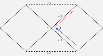
Figure 1: Scattering indicated for one incoming and outgoing particle of an eikonal process involving impact parameters smaller than $G_{N}M$. This process can be described on a Schwarzschild background with Schwarzschild radius $G_{N}M$. For impact parameters comparable to the Schwarzschild radius, the scattering is dominated by an eikonal process in the near-horizon region. Due to the small angle approximation, the region is about the bifurcation point O.

2.2 Near-horizon eikonal amplitude

The eikonal limit of trans-Planckian 2-2 scattering in flat spacetime, i.e., center-of-mass energy $\sqrt{s}$ is far larger than the Planckian mass $M_{PL}$ so that graviton exchanges dominate, requires a large impact parameter to suppress the transverse momentum transfer $q_{\perp}$. Besides, to avoid divergent results caused by gravitational collapse near the scattering center, the impact parameter $x_{\perp}\sim{\cal O}(\hbar/q_{\perp})$ should be far larger than the Schwarzschild radius associated with the center-of-mass energy, i.e., $x_{\perp}\gg G_{N}\sqrt{s}$ [56, 57]. The resultant eikonal amplitude (for massless particles) is [58, 59, 60]

$$i{\cal M}={i\kappa^{2}s^{2}\over q_{\perp}^{2}}{\Gamma(1-iG_{N}s)\over\Gamma(1+iG_{N}s)}\left({4\mu^{2}\over q_{\perp}^{2}}\right)^{-iG_{N}s}$$ (7)

with $\mu$ denoting an infrared cutoff. This amplitude has a semi-classical interpretation as 1-1 scattering of an ultra high energy massless particle against a null-like shockwave background which incorporates the backreaction [58]. This is consistent with the expectation of the eikonal limit, that is, the resummation of ladder graviton exchange results in a coherent background. Decomposing this eikonal amplitude in the partial-wave basis yields a unitary S-matrix for each mode represented by an eikonal phase,

$$\delta_{\ell}(s)={s\over 2}\log{\ell(\ell+1)\over s}\;.$$ (8)

This phase encodes the peculiar dynamics from the dominant soft graviton contributions in the ladder diagrams. Later, we will compare this phase to the one for the eikonal scattering in the near-horizon region.

From the discussion in the previous subsection, we see that the metric of the near-horizon region of the Schwarzschild black hole is approximately a flat metric with an implicit horizon scale in relation to the Rindler metric. This raises the possibility of formulating the eikonal scattering in the near-horizon region in a similar fashion to the approach on flat spacetime. Indeed, this idea had been proposed long ago [61, 62], and recently refined in further detail [45, 46, 47, 48, 63]. Due to being restricted about the near-horizon region, the kinematic constraints for eikonal scattering are quite different from those on flat spacetime. This especially concerns the impact parameter which is restricted to be $\ell_{PL}\ll x_{\perp}\approx R$, where $\ell_{PL}$ is the Planckian length and $R=2G_{N}M$ is the Schwarzschild radius. As shown in [46, 45], eikonal scattering (small angle scattering) in this regime requires $\sqrt{s}\gg\gamma M_{PL}$ with $M_{PL}$ the Planckian mass and $\gamma={M_{PL}\over M}$ an emerging dimensionless coupling between matter and graviton of the effective theory that results from integrating out the transverse directions. Due to the smallness of $\gamma$ for a typical macroscopic black hole, the new constraint on $s$ implies that the eikonal scattering can be non-Planckian in the near-horizon region. Consequently, this enables us to circumvent the breakdown of conventional eikonal techniques when dealing with scattering at small impact parameters.

The general picture that arises is the following. An eikonal scattering process that includes small impact parameters may be considered as a process on an asymptotically flat black hole spacetime. For impact parameters far larger than the Schwarzschild radius, we have the usual eikonal approximation with large impact parameters. However, as the impact parameter becomes comparable to that of the Schwarzschild radius, we have an eikonal scattering amplitude in the near-horizon regime, where the impact parameter is comparable to the Schwarzschild radius and with a phase dominated by the resummation over soft graviton modes. The eikonal amplitude including small impact parameters may thus be considered as a product over three amplitudes – from past infinity to the near-horizon region, the eikonal amplitude in the near-horizon region, and from the near-horizon region to future infinity. This is schematically depicted in Figure 1, and the amplitude that we will discuss is defined in the near-horizon region about the bifurcation point. In the following, we briefly review the derivation of the so-called “black hole eikonal phase” for near-horizon scattering with the aforementioned kinematic constraints on $x_{\perp}$ and $s$.

Starting with the Schwarzschild background metric given in 3,

$$ds^{2}_{NH}=g_{\mu\nu}dx^{\mu}dx^{\nu}=-2A(x^{-},x^{+})dx^{-}dx^{+}+r^{2}(x^{-},x^{+})d\Omega_{2}^{2}\;.$$ (9)

with

$$A(x^{-},x^{+})=2\frac{R}{r(x^{-},x^{+})}e^{1-\frac{r(x^{-},x^{+})}{R}}$$ (10)

we will consider the theory of linearized Einstein gravity minimally coupled with a massless scalar $\psi$ in this background,

$$S[h_{\mu\nu},\psi]=\int d^{4}x\sqrt{-g}~{}\Big{[}{1\over 4}R^{(1)}[h_{\mu\nu};g_{\mu\nu}]+\frac{1}{2}\psi~{}\Box\psi+\frac{1}{2}\kappa h^{\mu\nu}T_{\mu\nu}\Big{]}$$ (11)

where ${1\over 4}\sqrt{-g}~{}R^{(1)}[h_{\mu\nu};g_{\mu\nu}]$ is the $h_{\mu\nu}$-quadratic part of ${1\over 2\kappa^{2}}\sqrt{-(g+\kappa h)}~{}R[g_{\mu\nu}+\kappa h_{\mu\nu}]$, $\kappa=\sqrt{8\pi G_{N}}$, and $T_{\mu\nu}$ is the stress tensor of the scalar $\psi$

$$T_{\mu\nu}=\partial_{\mu}\psi\partial_{\nu}\psi-\frac{1}{2}g_{\mu\nu}g^{\rho\sigma}\partial_{\rho}\psi\partial_{\sigma}\psi\,.$$ (12)

Exploiting the background spherical symmetry one can decompose the metric and scalar fields in the partial-wave basis, i.e.,

$$h_{\mu\nu}=\sum_{\ell,m}h^{\text{odd}}_{\ell m,\mu\nu}Y^{m}_{\ell}+\sum_{\ell,m}h^{\text{even}}_{\ell m,\mu\nu}Y^{m}_{\ell}\;,\qquad\psi=\sum_{\ell,m}\psi_{\ell m}Y^{m}_{\ell}$$ (13)

with the additional choice of the usual Regge-Wheeler gauge,

$$h_{aA}^{\text{odd}}=-h_{a}\epsilon_{A}{}^{B}\partial_{B}Y^{m}_{\ell},\qquad h_{ab}^{\text{even}}=H_{ab}Y^{m}_{\ell},\qquad h_{AB}^{\text{even}}=K\gamma_{AB}Y^{m}_{\ell}$$ (14)

where $\gamma_{AB}$ and $\epsilon_{AB}$ are respectively the metric and Levi-Civita tensor on the 2-sphere, while $a,b$ are indices for the longitudinal null coordinates $x^{\pm}$. Spherical symmetry further ensures the decoupling of the even and odd modes. Moreover, the even parity nature of the scalar field yields no coupling to the odd modes from the interaction vertex. Therefore, only even parity graviton modes $K$ and $H_{ab}$ will be involved in the scattering of the massless scalar in the reduced theory.

Since the longitudinal part of the near-horizon metric is conformal to a flat metric, we can perform the following Weyl transformation and field redefinitions to yield canonical kinetic terms in the reduced theory

$$g_{ab}\rightarrow A(x^{-},x^{+})\eta_{ab},\qquad H_{ab}\rightarrow\frac{1}{r}A(x^{-},x^{+}){\mathbf{h}}_{ab},\qquad K\rightarrow\frac{1}{r}{\bf K},\qquad\psi\rightarrow\frac{1}{r}\phi\;,$$ (15)

which can be used to obtain a two-dimensional effective theory on integrating out the transverse degrees of freedom. By introducing a single traceless tensor mode, $\tilde{\mathbf{h}}^{ab}=\mathbf{h}^{ab}-\eta^{ab}({1\over 2}\mathbf{h}+{\bf K})$, for the 3-vertex coupling to two scalars, and carrying out a field redefinition $\tilde{{\bf K}}={\bf h}+\frac{2R^{2}}{\ell(\ell+1)+2}\left(\eta^{ab}\partial_{a}\partial_{b}-{1\over R^{2}}\ell(\ell+1)\right){\bf K}$, we can also remove the mixed contribution between ${\bf K}$ and $\mathbf{h}^{ab}$. However the corresponding graviton propagators are complicated due to the potentials arising from the Weyl scaling and field redefinitions 15. If we focus on the near-horizon region so that the metric becomes that of flat spacetime

$$A(x^{-},x^{+})\approx 1\;,\qquad\textrm{if}\quad r=R+{\cal O}(r-R)\;,$$ (16)

the resulting two-dimensional effective theory has considerably simpler properties. Upon Fourier transforming all the fields, the two-dimensional effective action takes on the following simple form [46, 48]:

$$S[\tilde{{\mathbf{h}}}^{ab},\tilde{{\bf K}},\phi] = {1\over 4}\int d^{2}k\;\Big{(}{\tilde{\mathbf{h}}}^{ab}{\bf P}^{-1}_{abcd}(k)\tilde{{\mathbf{h}}}^{cd}+\tilde{{\bf K}}{\bf P}^{-1}_{\bf K}\tilde{\bf K}\Big{)}+{1\over 2}\int d^{2}p\;\phi{\bf P}^{-1}_{\phi}(p)\phi$$ (17)

$$+\;\gamma\int d^{2}\Pi\;\tilde{\mathbf{h}}^{ab}(k)p_{1a}p_{2b}\phi_{0}(p_{1})\phi(p_{2})$$

where $d^{2}\Pi$ is a shorthand for $d^{2}kd^{2}p_{1}d^{2}p_{2}\;\delta^{(2)}(k+p_{1}+p_{2})$, and the dimensionless coupling for the 3-vertex is given by

$$\gamma:={\kappa\over R}={M_{PL}\over M}\;.$$ (18)

which arises due to considering a strict near-horizon limit. Note that one of the scalars in the 3-vertex is fixed to have zero angular momentum because the distributed angular momentum transfer among the external legs should be suppressed by the kinematics imposed by spherical symmetry. The propagators have the expressions

$${\bf P}_{\phi}(p)=\frac{1}{p^{2}+\mu^{2}-i\epsilon}\;,\qquad{\bf P}_{\bf K}=\frac{4R^{2}}{\ell(\ell+1)+2}\;,\qquad{\bf P}^{abcd}(k)={\bf P}^{abcd}_{\text{soft}}+{\bf P}^{abcd}_{\text{hard}}(k)\;,$$ (19)

where we decompose the tensor mode propagator into its soft ($k$-independent) and hard ($k$-dependent) parts as follows [48]:

$${\bf P}^{abcd}_{\text{soft}}=\frac{R^{2}}{\ell(\ell+1)+2}\left(\eta^{ab}\eta^{cd}-\eta^{ac}\eta^{bd}-\eta^{ad}\eta^{bc}\right)\;,$$ (20)

$${\bf P}^{abcd}_{\text{hard}}(k)=-\frac{\ell(\ell+1)+2}{\ell(\ell+1)-2}\frac{1}{k^{2}+\mu^{2}}(\eta^{ab}+k^{ab})(\eta^{cd}+k^{cd})$$ (21)

with

$$k^{ab}:=\frac{2R^{2}}{\ell(\ell+1)+2}(k^{a}k^{b}-{1\over 2}k^{2}\eta^{ab})\;.$$ (22)

The soft graviton exchange associated with ${\bf P}^{abcd}_{\text{soft}}$ will give a leading contribution to amplitudes. While integrating out the transverse part by using the orthogonality relations between spherical harmonics, all the fields in the effective field theory acquire an effective mass

$$\mu^{2}:={\ell(\ell+1)+1\over R^{2}}\;,$$ (23)

which can be thought of as an infrared regulator.

From the above effective theory in 17, we can obtain the Feynman rules to compute the amplitudes for the soft/hard graviton exchanges in 2-2 scattering of the scalar particles with two incoming momenta $p_{1}=(p_{1-},0)$ and $p_{2}=(0,p_{2+})$. This allows us to define the center-of-mass energy as,

$$s=-(p_{1}+p_{2})^{2}=2p_{1-}p_{2+}\;.$$ (24)

Since only the tensor mode is coupled to the scalars via 3-vertex, we just need to consider 2-2 scattering amplitude involving the exchange of tensor mode associated with graviton propagators ${\bf P}^{abcd}_{\text{hard}}$ and ${\bf P}^{abcd}_{\text{soft}}$. We denote the corresponding amplitudes as $M_{\rm hard}$ and $M_{\rm soft}$, respectively. Using the symmetry property: $k^{ab}=k^{ba}$ and $k^{ab}p_{1a}p_{2b}=0$ with our metric choice, one can find that

$$M_{\rm hard}\propto~{}{\gamma^{2}s^{2}\over s+\mu^{2}}\;.$$ (25)

and from the soft graviton exchange

$$M_{\rm soft}=(i\gamma p_{1a}p_{1b})(2{\bf P}^{abcd}_{\text{soft}})(i\gamma p_{2c}p_{2d})={\gamma^{2}R^{2}s^{2}\over(\ell^{2}+\ell+2)}\;.$$ (26)

Note that this soft amplitude is suppressed for large $\ell$, contrary to the large $\ell$ dominance of its counterpart in flat space. Two important properties can be inferred from the above results. Due to the effective mass involving the Schwarzschild radius, we have a modified regime for eikonal scattering in the near-horizon region

$$s\gg\mu^{2}\quad\textrm{or}\quad\sqrt{s}\gg\gamma M_{PL}\;.$$ (27)

In addition, in the large $s$ limit we always have

$${M_{\rm hard}\over M_{\rm soft}}\sim\mathcal{O}(s^{-1})\,.$$ (28)

Thus $M_{\rm hard}$ is a subleading contribution to $M_{\rm soft}$ in the large $s$ limit. As the soft graviton exchange dominates for all loop orders, we can re-sum the corresponding ladder diagrams to derive the leading contribution to the near-horizon eikonal amplitude [46]

$$iA^{\ell}_{\rm NH\;eikonal}=2s\left(e^{i\chi_{\ell}}-1\right)$$ (29)

where the associated eikonal phase is

$$\chi_{\ell}=\frac{\kappa^{2}s}{\ell^{2}+\ell+2}\;.$$ (30)

The $s$ and $\ell$ dependence of this phase differ from eikonal amplitudes on flat spacetimes 8. In the following section, we derive the four-dimensional description of this amplitude and its corresponding CCFT.

3 Near-horizon celestial eikonal amplitude

We will proceed by first deriving the four-dimensional near-horizon amplitude from the effective two-dimensional result discussed in the previous section. This requires summing over the partial wave result 30 in the small angle approximation using known techniques [64, 65]. We will then perform the Mellin transform on this momentum space amplitude to derive the near-horizon celestial amplitude.

3.1 Four-dimensional near-horizon eikonal amplitude from partial sum

The two-dimensional near-horizon eikonal amplitude result 29 can be used to derive a corresponding four-dimensional near-horizon eikonal amplitude in terms of a two-dimensional integral over transverse impact parameter space. We first define the partial wave amplitude from the eikonal phase $\chi_{\ell}$ given in 30,

$$f_{\text{NH eikonal}}=\frac{1}{2i\sqrt{s}}\sum_{\ell}(2\ell+1)\left(e^{i\chi_{\ell}}-1\right)P_{\ell}(\cos\theta)\,.$$ (31)

where $s$ is now the square of the center of mass energy in four-dimensional momentum space and $\theta$ is the angle between the incoming and scattered momenta. The four-dimensional amplitude, apart from the momentum conserving delta function, then follows from a known prescription for eikonal amplitudes [64] in the vanishing angle $\theta$ limit and is given by

$$A_{\text{NH eikonal}}=4\pi i\sqrt{s}f_{\text{NH eikonal}}\;.$$ (32)

The sum over $\ell$ in 31 can be traded for a two-dimensional integral over the transverse directions. This follows from the relation between the transverse direction and the angular momentum mode $\ell$ arising from the definition of angular momentum (squared) [66, 67]

$$\ell(\ell+1)=s|x_{\perp}|^{2}$$ (33)

Another ingredient is an integral representation for the Legendre polynomials for small-angle scattering. Thus we may always consider

$$P_{\ell}(\cos{\theta}) =\frac{1}{2\pi}\int_{0}^{2\pi}d\phi~{}\exp\left(i\,2\ell\sin\left(\frac{\theta}{2}\right)\cos{\phi}\right)\;,$$ (34)

$$\sin\left(\frac{\theta}{2}\right) =\frac{\sqrt{-t}}{2\sqrt{s}}=\frac{|p_{\perp}|}{2\sqrt{s}}\,,$$ (35)

where we used the known relation between Legendre polynomials and Bessel functions in the small angle approximation in 34, while 35 is the relation between the exchanged momentum and center of mass energy for small angle scattering.

On substituting 33 in 30, we find that the resultant eikonal phase receives its dominant contribution for large $\ell$ (or equivalently large $s$) and small $x_{\perp}$.

$$\exp(i\chi_{\ell})=\exp\left(\frac{i\kappa^{2}s}{s|x_{\perp}|^{2}+2}\right)$$ (36)

To illustrate the behavior of the phase we can carry out a perturbative expansion of 36 in the large $s$ approximation to find

$$\chi_{\ell}=\frac{\kappa^{2}}{|x_{\perp}|^{2}}+\mathcal{O}(s^{-1})\,,$$ (37)

which can be noted as differing from the corresponding graviton mediated eikonal amplitude on flat spacetime that grows with $s$ [60, 66] In the following, we retain the complete expression for the eikonal phase in 36, which capture all $\mathcal{O}(s^{-1})$ properties. However, as in all eikonal amplitudes, all corrections in the more subleading $\mathcal{O}\left(\sqrt{-\frac{t}{s}}\right)$ are ignored.

Substituting 33, 34 and 35 in 31, we find the partial wave amplitude result

$$f_{\text{NH eikonal}} =-\frac{i\sqrt{s}}{2\pi}\int d^{2}x_{\perp}\left[\exp\left(\frac{i\kappa^{2}s}{s|x_{\perp}|^{2}+2}\right)-1\right]e^{i\vec{p}_{\perp}.\vec{x}_{\perp}}+\mathcal{O}\left(\sqrt{-\frac{t}{s}}\right)\;.$$ (38)

Lastly, plugging back 38 in 32, we find the following result for the four-dimensional near-horizon eikonal amplitude

$$A_{\text{NH eikonal}}=2s\int d^{2}x_{\perp}\left[\exp\left(\frac{i\kappa^{2}s}{s|x_{\perp}|^{2}+2}\right)-1\right]e^{i\vec{p}_{\perp}.\vec{x}_{\perp}}\;.$$ (39)

This differs from the expression for the eikonal amplitude on asymptotically flat spacetimes through the eikonal phase. The two main differences lie in the dependence of the eikonal phase on $s$ and the impact parameter $x_{\perp}$. The eikonal phase for graviton-mediated scattering on asymptotically flat spacetimes grows with $s$ and holds for large impact parameters $x_{\perp}$, which is evident from substituting 8 in 33 [66]. In contrast, the subleading terms in the eikonal phase of the near-horizon scattering process decay with large $s$ (as indicated in 37) with the dominant contribution from $x_{\perp}\ll 1$ in units of the Schwarzschild radius. In other words, one can see from 37 that while we consider a high energy scattering process with $\frac{-t}{s}\ll 1$ near the horizon, the eikonal phase grows more dominant as we reduce the impact parameter. In the following subsection, we determine how this manifests in a celestial description and compare the result with the celestial eikonal amplitude on asymptotically flat spacetimes.

3.2 Near-horizon celestial eikonal amplitude

We have noted that the near-horizon geometry in the limit of approaching the horizon can be described by a flat spacetime metric. The near-horizon eikonal amplitude is a scattering process restricted to this region involving external massless plane wave states. Hence a near-horizon celestial description of this amplitude can result from a Mellin transform of the near-horizon eikonal amplitude through its action on the external states, following the same arguments as recently provided for flat spacetime eikonal amplitudes in [31].

We accordingly define the four-dimensional 2-2 near-horizon celestial eikonal amplitude as the Mellin transform of the near-horizon eikonal amplitude given in 39 including the momentum conserving delta function

$$\tilde{A}_{\text{NH eikonal}}=(2\pi)^{4}\left(\prod_{i=1}^{4}\int_{0}^{\infty}d\omega_{i}\omega_{i}^{\Delta_{i}-1}\right)A_{\text{NH eikonal}}~{}\delta^{(4)}\left(\sum_{i=1}^{4}p_{i}\right)\,.$$ (40)

We consider the momenta of the external states as considered in [31]. This involves an all-outgoing convention with

$$p_{i}=\eta_{i}\omega_{i}\hat{q}_{i}\;;\qquad i=1\,,\cdots 4$$ (41)

with $\eta_{i}=+1$ for the outgoing states $i=3,4$, $\eta_{i}=-1$ for the incoming states $i=1,2$, and $\hat{q}_{i}$ a null vector parameterized in terms of the following transverse and longitudinal components

$$\hat{q}_{i} =\left(1+q_{i}\,,q_{i,\perp}\,,1-q_{i}\right)=(1+z_{i}\bar{z}_{i},z_{i}+\bar{z}_{i},-i(z_{i}-\bar{z}_{i}),1-z_{i}\bar{z}_{i})\,,\qquad i=1,3$$ (42)

$$\hat{q}_{i} =\left(1+q_{i}\,,q_{i,\perp}\,,-1+q_{i}\right)={1\over z_{i}\bar{z}_{i}}(1+z_{i}\bar{z}_{i},z_{i}+\bar{z}_{i},-i(z_{i}-\bar{z}_{i}),1-z_{i}\bar{z}_{i})\,,\qquad i=2,4\,.$$ (43)

where ($z,\bar{z}$) is a point on the celestial sphere at the horizon. The massless condition $\hat{q}^{2}_{i}=0$ imposes $4q_{i}=|q_{i,\perp}|^{2}$, which relates the longitudinal component $q_{i}$ with the transverse component $q_{i,\perp}$, a two component vector. The constraints then turn into the expressions of $\hat{q}_{i}$’s in terms of $z_{i}$’s. Hence for an eikonal scattering process with $s\gg t$, we have $q_{i}\sim|q_{i,\perp}|^{2}\ll 1$, with $\omega_{1}\simeq\omega_{3}$ and $\omega_{2}\simeq\omega_{4}$. We use $\simeq$ to indicate an equivalence up to corrections subleading in $\mathcal{O}\left(q_{\perp}^{2}\right)$.

The above considerations for the external states further imply that for $i=1,3$ we have $p_{i}^{+}=p_{i}^{0}+p_{i}^{3}=2\eta_{i}\omega_{i}\gg p_{i,\perp}$ and $p_{i}^{-}=p_{i}^{0}-p_{i}^{3}\simeq 0$, while for $i=2,4$ we have $p_{i}^{-}=2\eta_{i}\omega_{i}\gg p_{i,\perp}$ and $p_{i}^{+}\simeq 0$. With the above definitions, the delta function in 40 takes the form

$$\delta^{(4)}\left(\sum_{i=1}^{4}p_{i}\right) =2\delta\left(p_{1}^{+}+p_{3}^{+}\right)\delta\left(p_{2}^{-}+p_{4}^{-}\right)\delta^{(2)}\left(\sum_{i=1}^{4}p_{i,\perp}\right)\;,$$

$$=\frac{1}{2}\delta\left(\omega_{1}-\omega_{3}\right)\delta\left(\omega_{2}-\omega_{4}\right)\delta^{(2)}\left(\sum_{i=1}^{4}\eta_{i}\omega_{i}q_{i,\perp}\right)\;.$$ (44)

Likewise, we have for the Mandelstam variables $s$ and $t$

$$s \simeq-2p_{1}^{+}p_{2}^{-}=4\omega_{1}\omega_{2}\;,$$

$$-t \simeq\left(p_{1,\perp}+p_{3,\perp}\right)^{2}=\left(\omega_{3}q_{3,\perp}-\omega_{1}q_{1,\perp}\right)^{2}\;.$$ (45)

Substituting 44 and 45 in 40, we get the following expression

$$\tilde{A}_{\text{NH Eikonal}} =4(2\pi)^{4}\int_{0}^{\infty}d\omega_{1}\int_{0}^{\infty}d\omega_{2}\,\omega_{1}^{\Delta_{1}+\Delta_{3}-1}\omega_{2}^{\Delta_{2}+\Delta_{4}-1}$$

$$\qquad\int d^{2}x_{\perp}\sum_{n=1}^{\infty}\frac{1}{n!}\left(\frac{i\kappa^{2}}{|x_{\perp}|^{2}+\frac{1}{2\omega_{1}\omega_{2}}}\right)^{n}e^{-i\omega_{1}q_{13,\perp}.x_{\perp}}\delta^{(2)}(\omega_{1}q_{13,\perp}+\omega_{2}q_{24,\perp})\,,$$ (46)

where we have written the eikonal phase as a series expansion and used the notation $q_{i,\perp}-q_{j,\perp}=q_{ij,\perp}$.

With the exponential representation for the two-dimensional delta function

$$\int d^{2}\bar{x}_{\perp}\exp\left(-ik\cdot\bar{x}_{\perp}\right)=(2\pi)^{2}\delta^{(2)}(k)\,,$$ (47)

we may express 46 as

$$\tilde{A}_{\text{NH Eikonal}} =4(2\pi)^{2}\int_{0}^{\infty}d\omega_{1}\int_{0}^{\infty}d\omega_{2}\,\omega_{1}^{\Delta_{1}+\Delta_{3}-1}\omega_{2}^{\Delta_{2}+\Delta_{4}-1}$$

$$\qquad\int d^{2}x_{\perp}\int d^{2}\bar{x}_{\perp}\sum_{n=1}^{\infty}\frac{1}{n!}\left(\frac{i\kappa^{2}}{|x_{\perp}|^{2}+\frac{1}{2\omega_{1}\omega_{2}}}\right)^{n}e^{-i\omega_{1}q_{13,\perp}.\left(x_{\perp}+\bar{x}_{\perp}\right)}e^{-i\omega_{2}q_{24,\perp}.\bar{x}_{\perp}}\,.$$ (48)

The second line in 48 can be further simplified. We first express all frequencies appearing in the eikonal phase as resulting from the action of celestial momentum operators on $\omega_{i}^{\Delta_{i}-1}$ for the incoming particles, $P_{i}^{\mu}=-\hat{q}_{i}^{\mu}e^{\partial_{\Delta_{i}}}$ for $i=1,2$ [8]. We can expand the eikonal phase as an infinite series

$$\left(|x_{\perp}|^{2}+\frac{1}{2\omega_{1}\omega_{2}}\right)^{-n}=\sum_{k=0}^{\infty}\;C_{n-1}^{k+n-1}x_{\perp}^{-2(n+k)}\left(-\frac{1}{2\omega_{1}\omega_{2}}\right)^{k}$$ (49)

with $C_{n-1}^{k+n-1}=\frac{(k+n-1)!}{k!(n-1)!}$. From the standard identity of the celestial momentum operator acting on the integrand of the Mellin transform [31, 8]

$$\omega_{1}^{\Delta_{1}+\Delta_{3}-1-k} =e^{-k\partial_{\Delta_{1}}}\omega_{1}^{\Delta_{1}+\Delta_{3}-1}\;,$$

$$\omega_{2}^{\Delta_{2}+\Delta_{4}-1-k} =e^{-k\partial_{\Delta_{2}}}\omega_{2}^{\Delta_{2}+\Delta_{4}-1}\;,$$ (50)

we have the relation

$$\left(\frac{i\kappa^{2}}{|x_{\perp}|^{2}+\frac{1}{2\omega_{1}\omega_{2}}}\right)^{n} \omega_{1}^{\Delta_{1}+\Delta_{3}-1}\omega_{2}^{\Delta_{2}+\Delta_{4}-1}$$

$$=\left(\frac{i\kappa^{2}}{|x_{\perp}|^{2}+\frac{1}{2}\exp(-\partial_{\Delta_{1}})\exp(-\partial_{\Delta_{2}})}\right)^{n}\omega_{1}^{\Delta_{1}+\Delta_{3}-1}\omega_{2}^{\Delta_{2}+\Delta_{4}-1}\;.$$ (51)

We hence see that a factor of $s=4\omega_{1}\omega_{2}$ can be interpreted as arising from the action of a shifting operator $4e^{\partial_{\Delta_{1}}}e^{\partial_{\Delta_{2}}}$ in the celestial basis following 3.2. We in addition consider the transformation $x_{\perp}+\bar{x}_{\perp}\to x_{\perp}$ resulting in an eikonal phase that depends on the transverse distance $x_{\perp}-\bar{x}_{\perp}$. By performing this transformation and using 51 in 48, we get the result

$$\tilde{A}_{\text{NH Eikonal}}=4(2\pi)^{2}\int d^{2}x_{\perp}\int d^{2}\bar{x}_{\perp}\sum_{n=1}^{\infty}\frac{1}{n!}\left(\frac{i\kappa^{2}}{|x_{\perp}-\bar{x}_{\perp}|^{2}+\frac{1}{2}\exp(-\partial_{\Delta_{1}})\exp(-\partial_{\Delta_{2}})}\right)^{n}$$

$$\qquad\qquad\qquad\int_{0}^{\infty}d\omega_{1}\omega_{1}^{\Delta_{1}+\Delta_{3}-1}e^{-i\omega_{1}q_{13,\perp}.x_{\perp}}\int_{0}^{\infty}d\omega_{2}\omega_{2}^{\Delta_{2}+\Delta_{4}-1}e^{-i\omega_{2}q_{24,\perp}.\bar{x}_{\perp}}$$

$$\qquad:=4(2\pi)^{2}\int d^{2}x_{\perp}\int d^{2}\bar{x}_{\perp}\left(e^{i\hat{\chi}_{\rm NH}}-1\right)\frac{i^{\Delta_{1}+\Delta_{3}}\Gamma\left(\Delta_{1}+\Delta_{3}\right)}{\left(-q_{13,\perp}\cdot x_{\perp}+i\epsilon\right)^{\Delta_{1}+\Delta_{3}}}\frac{i^{\Delta_{2}+\Delta_{4}}\Gamma\left(\Delta_{2}+\Delta_{4}\right)}{\left(-q_{24,\perp}\cdot\bar{x}_{\perp}+i\epsilon\right)^{\Delta_{2}+\Delta_{4}}}\,,$$ (52)

where in the last equation we defined the eikonal phase operator

$$\hat{\chi}_{\rm NH}:=\frac{\kappa^{2}}{|x_{\perp}-\bar{x}_{\perp}|^{2}+\frac{1}{2}\exp(-\partial_{\Delta_{1}})\exp(-\partial_{\Delta_{2}})}\;,$$ (53)

and made use of the identity

$$\int_{0}^{\infty}d\omega\omega^{\Delta-1}e^{-i\eta\omega q.x_{\perp}}=\frac{i^{\Delta}\Gamma\left(\Delta\right)}{\left(-q\cdot x_{\perp}+i\eta\epsilon\right)^{\Delta}}\;.$$ (54)

54 provides a definition of massless conformal primary wavefunctions for scattering on asymptotically flat spacetimes, while the form of 52 is very similar to the result for flat spacetime celestial eikonal amplitudes given in  [31]. The main difference with the flat spacetime result stems from the form of the eikonal phase operator 53. In [31] the eikonal phase operator for graviton mediated scattering takes the following form

$$\hat{\chi}_{\rm flat}\propto\kappa^{2}\exp(\partial_{\Delta_{1}})\exp(\partial_{\Delta_{2}})G_{\perp}(x_{\perp},\bar{x}_{\perp})$$ (55)

where $G_{\perp}(x_{\perp},\bar{x}_{\perp})$ is the transverse part of the propagator of exchange graviton. Comparing 53 and 55, we see that one difference concerns the action of $\exp(\partial_{\Delta_{1}})\exp(\partial_{\Delta_{2}})$, with the inverse dependence appearing in near-horizon eikonal amplitudes. In the following section, we will investigate 52 in more detail and compare our results with those of celestial eikonal amplitudes on asymptotically flat spacetimes.

4 Properties of the near-horizon celestial eikonal amplitude

Celestial amplitudes, on account of their involvement of boost eigenstates, are known to be sensitive to both UV and IR properties of scattering processes [20]. Lorentz and translation invariance on the celestial sphere further manifest in certain universal properties that celestial amplitudes must possess.

The near-horizon celestial eikonal amplitude 52 can be expanded as the sum of the Feynmann ladder diagrams, which are classified by the number of exchanged soft gravitons, i.e., denoted by $n$, or $(n-1)$ loops,

$$\tilde{A}_{\text{NH eikonal}}=\sum_{n=1}^{\infty}\tilde{A}_{\text{NH eikonal}}^{(n)}$$ (56)

with

$$\tilde{A}_{\text{NH eikonal}}^{(n)}=\frac{4(2\pi)^{2}}{n!}\int d^{2}x_{\perp}\int d^{2}\bar{x}_{\perp}\left(i\hat{\chi}_{\rm NH}\right)^{n}\frac{i^{\Delta_{1}+\Delta_{3}}\Gamma\left(\Delta_{1}+\Delta_{3}\right)}{\left(-q_{13,\perp}\cdot x_{\perp}+i\epsilon\right)^{\Delta_{1}+\Delta_{3}}}\frac{i^{\Delta_{2}+\Delta_{4}}\Gamma\left(\Delta_{2}+\Delta_{4}\right)}{\left(-q_{24,\perp}\cdot\bar{x}_{\perp}+i\epsilon\right)^{\Delta_{2}+\Delta_{4}}}\,.$$ (57)

The form of 57 is exact for all $n$. Below, we will argue that our result satisfies the expected universal properties of celestial amplitudes and is consistent with the defining properties of near-horizon eikonal amplitudes – that is it is mediated by soft graviton exchanges in the large $s$ limit.

We start with the integral representation of celestial eikonal amplitude from 46, incorporating the definition 56

$$\tilde{A}_{\text{NH eikonal}}^{(n)}= 4(2\pi)^{4}\int_{0}^{\infty}d\omega_{1}\omega_{1}^{\Delta_{1}+\Delta_{3}-1}\int_{0}^{\infty}d\omega_{2}\omega_{2}^{\Delta_{2}+\Delta_{4}-1}$$

$$\qquad\int d^{2}x_{\perp}\frac{1}{n!}\left(\frac{i\kappa^{2}}{|x_{\perp}|^{2}+\frac{1}{2\omega_{1}\omega_{2}}}\right)^{n}e^{-i\omega_{1}q_{13,\perp}\cdot x_{\perp}}\delta^{(2)}(\omega_{1}q_{13,\perp}+\omega_{2}q_{24,\perp})\;.$$ (58)

One of the properties of this celestial eikonal amplitude is that the integration over $x_{\perp}$ can be evaluated exactly to give the modified Bessel function of the second kind of integer order $n-1$,

$$\int d^{2}x_{\perp}\left(\frac{i\kappa^{2}}{|x_{\perp}|^{2}+\frac{1}{2\omega_{1}\omega_{2}}}\right)^{n}e^{-i\omega_{1}q_{13,\perp}\cdot x_{\perp}}=2\pi\frac{i^{n}\kappa^{2n}}{(n-1)!}\left(\omega_{1}|q_{13,\perp}|\sqrt{\frac{\omega_{1}\omega_{2}}{2}}\right)^{n-1}K_{n-1}\left(\sqrt{\frac{\omega_{1}}{2\omega_{2}}}|q_{13,\perp}|\right)$$ (59)

where we have used the known integral (cf 6.565.4 of [68])

$$\int_{0}^{\infty}\frac{J_{\nu}(bx)x^{\nu+1}}{(x^{2}+a^{2})^{\mu+1}}dx=\frac{a^{\nu-\mu}b^{\mu}}{2^{\mu}\Gamma(\mu+1)}K_{\nu-\mu}(ab),\quad-1<\text{Re}\,\nu<\text{Re}\,(2\mu+3/2);a,b>0\;.$$ (60)

Our analysis will be further considered in a center-of-mass frame with

$$|q_{\perp}|:=|q_{13,\perp}|=|q_{24,\perp}|\;,$$ (61)

Hence, on substituting 59 in 58 and performing the rescalings $\omega_{1}|q_{\perp}|\to\omega_{1}$ and $\omega_{2}|q_{\perp}|\to\omega_{2}$, we find

$$\tilde{A}_{\text{NH eikonal}}^{(n)}= 4(2\pi)^{5}\frac{i^{n}\kappa^{2n}}{n!(n-1)!}\left(|q_{\perp}|\right)^{-\beta-n-3}\int_{0}^{\infty}d\omega_{1}\omega_{1}^{\Delta_{1}+\Delta_{3}-1}\int_{0}^{\infty}d\omega_{2}\omega_{2}^{\Delta_{2}+\Delta_{4}-1}$$

$$\left(\omega_{1}\sqrt{\frac{\omega_{1}\omega_{2}}{2}}\right)^{n-1}K_{n-1}\left(\sqrt{\frac{\omega_{1}}{2\omega_{2}}}|q_{\perp}|\right)\delta^{(2)}(\omega_{1}n_{13,\perp}+\omega_{2}n_{24,\perp})\;,$$ (62)

where we defined the two dimensional vectors

$$n_{13,\perp}=(n_{13,\perp}^{1},n_{13,\perp}^{2}):={q_{13,\perp}\over|q_{\perp}|}\;,\qquad n_{24,\perp}=(n_{24,\perp}^{1},n_{24,\perp}^{2}):={q_{24,\perp}\over|q_{\perp}|}\;,$$ (63)

and

$$\beta:=\Delta_{1}+\Delta_{2}+\Delta_{3}+\Delta_{4}-4.$$ (64)

To further simplify 62, we consider the 2-2 scattering in the center of mass frame with the following parametrization for the transverse momenta in terms of the cross-ratio $z={-t\over s}$ [31],

$$q_{13,\perp}=(-(\sqrt{z}+\sqrt{\bar{z}}),i(\sqrt{z}-\sqrt{\bar{z}}))\;, \quad q_{24,\perp}=(\sqrt{z}+\sqrt{\bar{z}},i(\sqrt{z}-\sqrt{\bar{z}}))\;,$$ (65)

so that

$$|q_{\perp}|=2\sqrt{|z|}\;,\qquad n_{24,\perp}^{1}n_{13,\perp}^{2}=i\frac{z-\bar{z}}{|q_{\perp}|^{2}}=-n_{24,\perp}^{2}n_{13,\perp}^{1}\;.$$ (66)

In the parametrization of $\hat{q}_{i}$ of 42 and 43, this corresponds to the choice

$$z_{1}=0,\quad z_{2}=\infty,\quad z_{3}=\sqrt{z},\quad z_{4}=-{1\over\sqrt{z}}\;,$$ (67)

such that in the eikonal limit,

$$z={-t\over s}\approx{z_{13}z_{24}\over z_{12}z_{34}}\ll 1\;.$$ (68)

The two-dimensional delta function $\delta^{(2)}(\omega_{1}n_{13,\perp}+\omega_{2}n_{24,\perp})$ can be factored into a product of delta functions [31]

$$\delta^{(2)}(\omega_{1}n_{13,\perp}+\omega_{2}n_{24,\perp}) =\frac{1}{\omega_{1}}\delta\left(\omega_{2}+\omega_{1}\frac{n_{24,\perp}^{1}}{n_{13,\perp}^{1}}\right)\delta(n_{24,\perp}^{1}n_{13,\perp}^{2}-n_{24,\perp}^{2}n_{13,\perp}^{1})\;,$$

$$=\frac{|q_{\perp}|^{2}}{2\omega_{1}}\delta\left(\omega_{2}-\omega_{1}\right)\delta(z-\bar{z})\;,$$ (69)

where in the second line of 69 we made use of 65 and 66, along with the standard scaling property of the Dirac delta function. On carrying out the integral over $\omega_{2}$ in 62 and using $\delta(z-\bar{z})$ to write $|q_{\perp}|=2\sqrt{z}$, we find

$$\tilde{A}_{\text{NH eikonal}}^{(n)}= 2(2\pi)^{5}\frac{i^{n}\kappa^{2n}2^{-\beta-2}}{n!(n-1)!}2^{\frac{3}{2}(1-n)}K_{n-1}(\sqrt{2z})\left(\sqrt{z}\right)^{-\beta-n-1}\delta(z-\bar{z})\int_{0}^{\infty}d\omega_{1}\omega_{1}^{\beta+2n-1}\;.$$ (70)

Lastly, we can perform the $\omega_{1}$ integral by analytically continuing to the regime of large scaling dimension $\Delta_{i}\gg 1$ with the following result [17]

$$\int_{0}^{\infty}d\omega_{1}\omega_{1}^{\beta+2n-1}:=\bm{\delta}(i(\beta+2n))\;.$$ (71)

Thus the integral in 71 is well defined when we set $\beta=-2n+ib$. Hence, on substituting 71 in 70 we arrive at the final result

$$\tilde{A}_{\text{NH eikonal}}^{(n)}= 2(2\pi)^{6}\frac{i^{n}\kappa^{2n}2^{-\beta-2}}{n!(n-1)!}2^{\frac{3}{2}(1-n)}K_{n-1}(\sqrt{2z})\left(\sqrt{z}\right)^{-\beta-n-1}\delta(z-\bar{z})\bm{\delta}(i(\beta+2n))\;.$$ (72)

The contribution $2^{-\beta-2}\delta(z-\bar{z})$ in 72 is part of the universal kinematic contribution in all celestial amplitudes [21, 31]. The delta function over $z$ in particular manifests translation invariance on the celestial sphere. The scaling behavior of the amplitude will follow from $\left(\sqrt{z}\right)^{-\beta-n-1}K_{n-1}(\sqrt{2z})$, which as we now show, has a universal $n$-independent leading scaling behavior for all $\tilde{A}_{\text{NH eikonal}}^{(n\geq 2)}$. The leading contribution of $K_{n-1}(\sqrt{2z})$ at each order $n$ is given by

$$K_{n-1}(\sqrt{2z}) \approx-\frac{1}{2}(-\sqrt{2z})^{n-1}\partial_{z}^{n-1}\ln\left(\frac{z}{2}\right)\;.$$ (73)

We consider 73 in 72 at tree level ($n=1$) and higher loops more generally ($n\geq 2$). For the tree-level exchange, we find

$$\tilde{A}_{\text{NH eikonal}}^{(1)} =-(2\pi)^{6}i\kappa^{2}2^{-\beta-2}\ln\left(\frac{z}{2}\right)\left(\sqrt{z}\right)^{-\beta-2}\delta(z-\bar{z})\bm{\delta}(i(\beta+2))+\cdots\,,$$

$$=-(2\pi)^{6}i\kappa^{2}\ln\left(\frac{z}{2}\right)\delta(z-\bar{z})\bm{\delta}(i(\beta+2))+\mathcal{O}\left(\sqrt{z}\right)\,,$$ (74)

where we utilized $\bm{\delta}(i(\beta+2))$ in the second line of 74 and $\cdots$ in the first line represent contributions subleading in small $z$. The tree-level exchange is hence dominated by $z^{0}\ln z$. Similarly, for $n\geq 2$ by using 73 and $\bm{\delta}(i(\beta+2n))$ in 72, we find the result to be

$$\tilde{A}_{\text{NH eikonal}}^{(n\geq 2)} =(2\pi)^{6}\frac{i^{n}\kappa^{2n}}{(n-1)n!}2^{-\beta-(n+3)}\left(\sqrt{z}\right)^{-\beta-2(n+1)}\delta(z-\bar{z})\bm{\delta}(i(\beta+2n))+\cdots\,,$$

$$=(2\pi)^{6}\frac{i^{n}\kappa^{2n}}{(n-1)n!}2^{n-3}z^{-1}\delta(z-\bar{z})\bm{\delta}(i(\beta+2n))+\mathcal{O}\left(\left(\sqrt{z}\right)^{-1}\right)\;.$$ (75)

We hence find the universal leading behavior of $z^{-1}$ for all $n\geq 2$ loop orders in the near-horizon celestial eikonal amplitude. It is quite interesting to consider the dynamical interpretation of the factor $\bm{\delta}(i(\beta+2n))$ in 72. Recall that the same pole structures are also proposed and discussed for the celestial amplitudes of IR or UV soft theories [20]. For the IR soft ones, these poles appear after Mellin transforming the IR expansion of the amplitude in the momentum basis, i.e., $\sum_{n=0}^{\infty}a_{n}^{\rm IR}\omega^{2n}$. In a UV soft theory, such as string theory, the UV behavior is softened by the productions of Hagedorn stringy states, which can be understood as the microscopic black holes by the string/black hole correspondence [51, 52, 53]. This implies that the celestial amplitudes can capture both non-perturbative physics in both UV and IR sides through the characteristics of $\beta=-2n$ poles. In our case, we are considering the celestial eikonal amplitudes for which the $\beta=-2n$ appears with $n$ labeling the order of the loop/ladder diagrams. Thus, a natural interpretation of these poles is the dominance of the soft graviton exchanges, with $n$ corresponding to the number of soft gravitons appearing in the ladder diagrams. An additional consequence is the absence of poles for $\text{Re}\,\beta>0$ in a manner analogous to UV soft theories. In this sense, these poles are the manifestation of the IR divergence due to soft graviton exchanges in the near-horizon region. This implies that celestial amplitudes can capture non-perturbative effects of strong gravity due to either black hole production or the existence of an event horizon.

5 Summary and Conclusion

Eikonal amplitudes provide an important class of non-perturbative scattering processes that have been recently investigated in the celestial basis. In this paper, we considered the celestial description of eikonal amplitudes past the critical length scale for the impact parameter, which is taken to be large in the usual eikonal approximation. In this regime, the leading approximation to the eikonal amplitude is governed by a resummation over soft graviton exchanges in the near-horizon geometry of a Schwarzschild black hole. Hence, near-horizon celestial eikonal amplitudes provide an interesting case of non-perturbative scattering processes in the boost eigenbasis beyond those on flat spacetime.

The near-horizon eikonal amplitude [45, 46, 47] accounts for the leading backreaction about a Schwarzschild background and is a two-dimensional result following the integration over spherical harmonics. The resulting eikonal phase 30 is dominated by small $\ell$ modes and transverse directions $x_{\perp}$. In section 3 we first derived the corresponding four-dimensional eikonal amplitude through a partial sum of the two-dimensional result and subsequently performed a Mellin transform on the external states to derive the near-horizon celestial eikonal amplitude. The conformal primary wavefunctions describing the external states are the same as those for the celestial eikonal amplitude on flat spacetimes, which follows from the isometries of the near-horizon region in the small angle approximation being identical to those on flat spacetimes. However, the eikonal phase, which captures the interactions of the external states with the exchanged gravitons near the horizon, crucially differs from the flat spacetime eikonal phase. More specifically, the four-dimensional near-horizon eikonal amplitude is defined from impact parameters comparable to the Schwarzschild radius and a perturbative series in $s^{-1}$ around $s$ being infinite. This manifests the property that the near-horizon eikonal amplitude is mediated by soft graviton modes.

In section 4 we investigated the near-horizon celestial eikonal amplitude to derive the main results of our paper, namely an exact all-loop order result for the celestial amplitude. The result involves universal kinematic factors of celestial amplitudes on flat spacetime. This is expected from our consideration of the near-horizon region in the small angle approximation, which simply provides a flat spacetime for the scattering process. However, the dynamical content of the celestial amplitude differs considerably from celestial amplitudes on flat spacetime. One of these differences follows from the $\bm{\delta}(i(\beta+2n))$ contribution. While this behavior is consistent with the expectation of soft UV behavior in CCFT, the near-horizon celestial eikonal amplitude provides the specific representation of exchanged soft gravitons with loop order $n$. We, in addition, have a $\sqrt{z}^{-\beta-n-1}K_{n-1}(\sqrt{2z})$ term as an all-loop order contribution from the near-horizon eikonal phase. This term on expanding about $z\ll 1$, and in conjunction with $\bm{\delta}(i(\beta+2n))$, provides a universal leading $n$-independent behaviour for $\sqrt{z}$. Thus, the leading scaling behavior of the cross-ratio $z$ in the celestial amplitude result is independent of loop order.

There are several further avenues to explore in the context of near-horizon amplitudes. It will be interesting to go beyond the small angle approximation used for the near-horizon background. In particular, we expect a correction to the $2$-sphere part of the metric in 1, which are also known to influence near-horizon symmetries [69, 70, 71]. We expect the consideration of near-horizon eikonal amplitudes past the leading approximation at large $R$ to be useful in understanding the manifestation of near-horizon symmetries in celestial amplitudes. In addition, it will also be important to better understand the celestial correspondence between the 1-1 scattering of a massless scalar field on a shockwave background and the 2-2 graviton-mediated eikonal amplitude for massless external scalar fields. We expect this correspondence to hold for the near-horizon eikonal amplitude upon considering a shockwave in the near-horizon region.

Acknowledgement :

The work of KF is supported by Taiwan’s NSTC with grant numbers 111-2811-M-003-005 and 112-2811-M-003 -003-MY3. The work of FLL is supported by Taiwan’s NSTC with grant numbers 109-2112-M-003-007-MY3 and 112-2112-M-003-006-MY3. The work of AM is supported by the Ministry of Education, Science, and Technology (NRF- 2021R1A2C1006453) of the National Research Foundation of Korea (NRF).

References

- [1] C. Cheung, A. de la Fuente and R. Sundrum, 4D scattering amplitudes and asymptotic symmetries from 2D CFT, JHEP 01 (2017) 112, [1609.00732].
- [2] S. Pasterski, S.-H. Shao and A. Strominger, Flat Space Amplitudes and Conformal Symmetry of the Celestial Sphere, Phys. Rev. D 96 (2017) 065026, [1701.00049].
- [3] S. Pasterski and S.-H. Shao, Conformal basis for flat space amplitudes, Phys. Rev. D 96 (2017) 065022, [1705.01027].
- [4] S. Pasterski, S.-H. Shao and A. Strominger, Gluon Amplitudes as 2d Conformal Correlators, Phys. Rev. D 96 (2017) 085006, [1706.03917].
- [5] C. Cardona and Y.-t. Huang, S-matrix singularities and CFT correlation functions, JHEP 08 (2017) 133, [1702.03283].
- [6] L. Donnay, A. Puhm and A. Strominger, Conformally Soft Photons and Gravitons, JHEP 01 (2019) 184, [1810.05219].
- [7] S. Stieberger and T. R. Taylor, Strings on Celestial Sphere, Nucl. Phys. B 935 (2018) 388–411, [1806.05688].
- [8] S. Stieberger and T. R. Taylor, Symmetries of Celestial Amplitudes, Phys. Lett. B 793 (2019) 141–143, [1812.01080].
- [9] M. Pate, A.-M. Raclariu and A. Strominger, Conformally Soft Theorem in Gauge Theory, Phys. Rev. D 100 (2019) 085017, [1904.10831].
- [10] A. Puhm, Conformally Soft Theorem in Gravity, JHEP 09 (2020) 130, [1905.09799].
- [11] M. Pate, A.-M. Raclariu, A. Strominger and E. Y. Yuan, Celestial operator products of gluons and gravitons, Rev. Math. Phys. 33 (2021) 2140003, [1910.07424].
- [12] D. Nandan, A. Schreiber, A. Volovich and M. Zlotnikov, Celestial Amplitudes: Conformal Partial Waves and Soft Limits, JHEP 10 (2019) 018, [1904.10940].
- [13] A. Fotopoulos, S. Stieberger, T. R. Taylor and B. Zhu, Extended BMS Algebra of Celestial CFT, JHEP 03 (2020) 130, [1912.10973].
- [14] S. Banerjee, S. Ghosh and R. Gonzo, BMS symmetry of celestial OPE, JHEP 04 (2020) 130, [2002.00975].
- [15] A. Fotopoulos, S. Stieberger, T. R. Taylor and B. Zhu, Extended Super BMS Algebra of Celestial CFT, JHEP 09 (2020) 198, [2007.03785].
- [16] H. A. González, A. Puhm and F. Rojas, Loop corrections to celestial amplitudes, Phys. Rev. D 102 (2020) 126027, [2009.07290].
- [17] L. Donnay, S. Pasterski and A. Puhm, Asymptotic Symmetries and Celestial CFT, JHEP 09 (2020) 176, [2005.08990].
- [18] S. Pasterski and A. Puhm, Shifting spin on the celestial sphere, Phys. Rev. D 104 (2021) 086020, [2012.15694].
- [19] R. Gonzo, T. McLoughlin and A. Puhm, Celestial holography on Kerr-Schild backgrounds, JHEP 10 (2022) 073, [2207.13719].
- [20] N. Arkani-Hamed, M. Pate, A.-M. Raclariu and A. Strominger, Celestial amplitudes from UV to IR, JHEP 08 (2021) 062, [2012.04208].
- [21] A. Atanasov, W. Melton, A.-M. Raclariu and A. Strominger, Conformal block expansion in celestial CFT, Phys. Rev. D 104 (2021) 126033, [2104.13432].
- [22] A. Guevara, E. Himwich, M. Pate and A. Strominger, Holographic symmetry algebras for gauge theory and gravity, JHEP 11 (2021) 152, [2103.03961].
- [23] A. Atanasov, A. Ball, W. Melton, A.-M. Raclariu and A. Strominger, (2, 2) Scattering and the celestial torus, JHEP 07 (2021) 083, [2101.09591].
- [24] A. Strominger, w(1+infinity) and the Celestial Sphere, 2105.14346.
- [25] A. Strominger, Algebra and the Celestial Sphere: Infinite Towers of Soft Graviton, Photon, and Gluon Symmetries, Phys. Rev. Lett. 127 (2021) 221601.
- [26] S. Pasterski, M. Pate and A.-M. Raclariu, Celestial Holography, in Snowmass 2021, 11, 2021. 2111.11392.
- [27] S. Pasterski, Lectures on celestial amplitudes, Eur. Phys. J. C 81 (2021) 1062, [2108.04801].
- [28] A.-M. Raclariu, Lectures on Celestial Holography, 2107.02075.
- [29] E. Crawley, N. Miller, S. A. Narayanan and A. Strominger, State-operator correspondence in celestial conformal field theory, JHEP 09 (2021) 132, [2105.00331].
- [30] L. Donnay, A. Fiorucci, Y. Herfray and R. Ruzziconi, Carrollian Perspective on Celestial Holography, Phys. Rev. Lett. 129 (2022) 071602, [2202.04702].
- [31] L. P. de Gioia and A.-M. Raclariu, Eikonal approximation in celestial CFT, JHEP 03 (2023) 030, [2206.10547].
- [32] S. Pasterski and H. Verlinde, Chaos in celestial CFT, JHEP 08 (2022) 106, [2201.01630].
- [33] T. McLoughlin, A. Puhm and A.-M. Raclariu, The SAGEX review on scattering amplitudes chapter 11: soft theorems and celestial amplitudes, J. Phys. A 55 (2022) 443012, [2203.13022].
- [34] E. Casali, W. Melton and A. Strominger, Celestial amplitudes as AdS-Witten diagrams, JHEP 11 (2022) 140, [2204.10249].
- [35] S. Mizera and S. Pasterski, Celestial geometry, JHEP 09 (2022) 045, [2204.02505].
- [36] J. Cotler, N. Miller and A. Strominger, An integer basis for celestial amplitudes, JHEP 08 (2023) 192, [2302.04905].
- [37] L. Donnay, G. Giribet, H. González, A. Puhm and F. Rojas, Celestial open strings at one-loop, 2307.03551.
- [38] A. Strominger, On BMS Invariance of Gravitational Scattering, JHEP 07 (2014) 152, [1312.2229].
- [39] A. Strominger and A. Zhiboedov, Gravitational Memory, BMS Supertranslations and Soft Theorems, JHEP 01 (2016) 086, [1411.5745].
- [40] D. Kapec, V. Lysov, S. Pasterski and A. Strominger, Semiclassical Virasoro symmetry of the quantum gravity -matrix, JHEP 08 (2014) 058, [1406.3312].
- [41] D. Kapec, P. Mitra, A.-M. Raclariu and A. Strominger, 2D Stress Tensor for 4D Gravity, Phys. Rev. Lett. 119 (2017) 121601, [1609.00282].
- [42] A. Strominger, Lectures on the Infrared Structure of Gravity and Gauge Theory, 1703.05448.
- [43] H. T. Lam and S.-H. Shao, Conformal Basis, Optical Theorem, and the Bulk Point Singularity, Phys. Rev. D 98 (2018) 025020, [1711.06138].
- [44] G. ’t Hooft, The Scattering matrix approach for the quantum black hole: An Overview, Int. J. Mod. Phys. A 11 (1996) 4623–4688, [gr-qc/9607022].
- [45] N. Gaddam, N. Groenenboom and G. ’t Hooft, Quantum gravity on the black hole horizon, JHEP 01 (2022) 023, [2012.02357].
- [46] N. Gaddam and N. Groenenboom, Soft graviton exchange and the information paradox, 2012.02355.
- [47] P. Betzios, N. Gaddam and O. Papadoulaki, Black hole S-matrix for a scalar field, JHEP 07 (2021) 017, [2012.09834].
- [48] N. Gaddam and N. Groenenboom, A toolbox for black hole scattering, 2207.11277.
- [49] D. Amati, M. Ciafaloni and G. Veneziano, Higher Order Gravitational Deflection and Soft Bremsstrahlung in Planckian Energy Superstring Collisions, Nucl. Phys. B 347 (1990) 550–580.
- [50] S. Weinberg, Infrared photons and gravitons, Phys. Rev. 140 (1965) B516–B524.
- [51] L. Susskind, Some speculations about black hole entropy in string theory, hep-th/9309145.
- [52] G. T. Horowitz and J. Polchinski, A Correspondence principle for black holes and strings, Phys. Rev. D 55 (1997) 6189–6197, [hep-th/9612146].
- [53] F.-L. Lin, T. Matsuo and D. Tomino, Hagedorn Strings and Correspondence Principle in AdS(3), JHEP 09 (2007) 042, [0705.4514].
- [54] I. Sachs and S. N. Solodukhin, Horizon holography, Phys. Rev. D 64 (2001) 124023, [hep-th/0107173].
- [55] G. W. Gibbons and C. M. Warnick, Universal properties of the near-horizon optical geometry, Phys. Rev. D 79 (2009) 064031, [0809.1571].
- [56] G. Veneziano, String-theoretic unitary S-matrix at the threshold of black-hole production, JHEP 11 (2004) 001, [hep-th/0410166].
- [57] D. Amati, M. Ciafaloni and G. Veneziano, Towards an S-matrix description of gravitational collapse, JHEP 02 (2008) 049, [0712.1209].
- [58] G. ’t Hooft, Graviton Dominance in Ultrahigh-Energy Scattering, Phys. Lett. B 198 (1987) 61–63.
- [59] D. Amati, M. Ciafaloni and G. Veneziano, Classical and Quantum Gravity Effects from Planckian Energy Superstring Collisions, Int. J. Mod. Phys. A 3 (1988) 1615–1661.
- [60] D. N. Kabat and M. Ortiz, Eikonal quantum gravity and Planckian scattering, Nucl. Phys. B 388 (1992) 570–592, [hep-th/9203082].
- [61] T. Dray and G. ’t Hooft, The Gravitational Shock Wave of a Massless Particle, Nucl. Phys. B 253 (1985) 173–188.
- [62] T. Dray and G. ’t Hooft, The Effect of Spherical Shells of Matter on the Schwarzschild Black Hole, Commun. Math. Phys. 99 (1985) 613–625.
- [63] F. Feleppa, N. Gaddam and N. Groenenboom, Charged particle scattering near the horizon, 2309.05791.
- [64] M. Levy and J. Sucher, Eikonal approximation in quantum field theory, Phys. Rev. 186 (1969) 1656–1670.
- [65] Y. F. Bautista, A. Guevara, C. Kavanagh and J. Vines, Scattering in black hole backgrounds and higher-spin amplitudes. Part I, JHEP 03 (2023) 136, [2107.10179].
- [66] H. L. Verlinde and E. P. Verlinde, Scattering at Planckian energies, Nucl. Phys. B 371 (1992) 246–268, [hep-th/9110017].
- [67] E. P. Verlinde and H. L. Verlinde, High-energy scattering in quantum gravity, Class. Quant. Grav. 10 (1993) S175–S184.
- [68] I. S. Gradshteyn and I. M. Ryzhik, Table of Integrals, Series, and Products; Seventh Edition. 2007.
- [69] L. Donnay, G. Giribet, H. A. Gonzalez and M. Pino, Supertranslations and Superrotations at the Black Hole Horizon, Phys. Rev. Lett. 116 (2016) 091101, [1511.08687].
- [70] L. Donnay, G. Giribet, H. A. González and M. Pino, Extended Symmetries at the Black Hole Horizon, JHEP 09 (2016) 100, [1607.05703].
- [71] D. Grumiller, A. Pérez, M. M. Sheikh-Jabbari, R. Troncoso and C. Zwikel, Spacetime structure near generic horizons and soft hair, Phys. Rev. Lett. 124 (2020) 041601, [1908.09833].