Pre-Training and Fine-Tuning
Generative Flow Networks

Abstract

Generative Flow Networks (GFlowNets) are amortized samplers that learn stochastic policies to sequentially generate compositional objects from a given unnormalized reward distribution. They can generate diverse sets of high-reward objects, which is an important consideration in scientific discovery tasks. However, as they are typically trained from a given extrinsic reward function, it remains an important open challenge about how to leverage the power of pre-training and train GFlowNets in an unsupervised fashion for efficient adaptation to downstream tasks. Inspired by recent successes of unsupervised pre-training in various domains, we introduce a novel approach for reward-free pre-training of GFlowNets. By framing the training as a self-supervised problem, we propose an outcome-conditioned GFlowNet (OC-GFN) that learns to explore the candidate space. Specifically, OC-GFN learns to reach any targeted outcomes, akin to goal-conditioned policies in reinforcement learning. We show that the pre-trained OC-GFN model can allow for a direct extraction of a policy capable of sampling from any new reward functions in downstream tasks. Nonetheless, adapting OC-GFN on a downstream task-specific reward involves an intractable marginalization over possible outcomes. We propose a novel way to approximate this marginalization by learning an amortized predictor enabling efficient fine-tuning. Extensive experimental results validate the efficacy of our approach, demonstrating the effectiveness of pre-training the OC-GFN, and its ability to swiftly adapt to downstream tasks and discover modes more efficiently. This work may serve as a foundation for further exploration of pre-training strategies in the context of GFlowNets.

1 Introduction

Unsupervised learning on large stores of data on the internet has resulted in significant advances in a variety of domains (Howard and Ruder, 2018, Devlin et al., 2018, Radford et al., 2019, Henaff, 2020). Pre-training with unsupervised objectives, such as next-token prediction in auto-regressive language models (Radford et al., 2019), on large-scale unlabelled data enables the development of models that can be effectively fine-tuned for novel tasks using few samples (Brown et al., 2020). Unsupervised learning at scale allows models to learn good representations, which enables data-efficient adaptation to novel tasks, and is central to the recent development towards larger models.

On the other hand, in the context of amortized inference, Generative Flow Networks (GFlowNets; Bengio et al., 2021) enable learning generative models for sampling from high-dimensional distributions over discrete compositional objects. Inspired by reinforcement learning (RL), GFlowNets learn a stochastic policy to sequentially generate compositional objects with a probability proportional to a given reward, instead of reward maximization. Therefore, GFlowNets have found success in applications to scientific discovery problems to generate high-quality and diverse candidates (Bengio et al., 2021, Jain et al., 2023a, b) as well as alternatives to Monte-Carlo Markov chains and variational inference for modeling Bayesian posteriors (Deleu et al., 2022, van Krieken et al., 2022).

As a motivating example, consider the drug discovery pipeline. A GFlowNet can be trained to generate candidate RNA sequences that bind to a target using as reward the binding affinity of the RNA sequence with the target (Lorenz et al., 2011, Sinai et al., 2020) (which can be uncertain and imperfect based on the current understanding of the biological system and available experimental data). However, there is no way to efficiently adapt the GFlowNet to sample RNA sequences binding to a different target of interest that reflects new properties. Unlike human intelligence, GFlowNets currently lack the ability to leverage previously learned knowledge to efficiently adapt to new tasks with unseen reward functions, and need to be trained from scratch to learn a policy for matching the given extrinsic reward functions for different tasks. Inspired by the success of the unsupervised pre-training and fine-tuning paradigm in vision, language, and RL (Jaderberg et al., 2016, Sekar et al., 2020) domains, it is natural to ask how can this paradigm benefit GFlowNets. As a step in this direction, we propose a fundamental approach to realize this paradigm for GFlowNets.

In this paper, we propose a novel method for reward-free unsupervised pre-training of GFlowNets. We formulate the problem of pre-training GFlowNets as a self-supervised problem of learning an outcome-conditioned GFlowNet (OC-GFN) which learns to reach any outcome (goal) as a functional understanding of the environment (akin to goal-conditioned RL (Chebotar et al., 2021)). The reward for training this OC-GFN is defined as the success of reaching the outcome. Due to the inherent sparse nature of this task-agnostic reward, it introduces critical challenges for efficient training OC-GFN in complex domains, particularly with higher-dimensional outcomes and long-horizon problems, since it is difficult to reach the outcome to get a meaningful reward signal. To tackle these challenges, we introduce a novel contrastive learning procedure to train OC-GFN to effectively handle such sparse rewards, which induces an implicit curriculum for efficient learning that resembles goal relabeling (Andrychowicz et al., 2017). To enable efficient learning in long-horizon tasks, we further propose a goal teleportation scheme to effectively propagate the learning signal to each step.

A remarkable result is that one can directly convert this pre-trained OC-GFN to sample proportionally to a new reward function for downstream tasks (Bengio et al., 2023). It is worth noting that in principle, this can be achieved even without re-training the policy, which is usually required for fine-tuning in RL, as it only learns a reward-maximizing policy that may discard many useful information. Adapting the pre-trained OC-GFN model to a new reward function, however, involves an intractable marginalization over possible outcomes. We propose a novel alternative by learning a predictor that amortizes this marginalization, allowing efficient fine-tuning of the OC-GFN to downstream tasks. Our key contributions can be summarized as follows:

• We propose reward-free pre-training for GFlowNets as training outcome-conditioned GFlowNet (OC-GFN) that learns to sample trajectories to reach any outcome.

• We investigate how to leverage the pre-trained OC-GFN model to adapt to downstream tasks with new rewards, and we also introduce an efficient method to learn an amortized predictor to approximate an intractable marginal required for fine-tuning the pre-trained OC-GFN model.

• Through extensive experiments on the GridWorld domain, we empirically validate the efficacy of the proposed pre-training and fine-tuning paradigm. We also demonstrate its scalability to larger-scale and challenging biological sequence design tasks, which achieves consistent and substantial improvements over strong baselines, especially in terms of diversity of the generated samples.

2 Preliminaries

Given a space of compositional objects $\mathcal{X}$, and a non-negative reward function $R:\mathcal{X}\mapsto\mathbb{R}^{+}$, the GFlowNet policy $\pi$ is trained towards sampling objects $x\in\mathcal{X}$ from the distribution defined by $R(x)$, i.e., $\pi(x)\propto R(x)$. The compositional objects are each sampled sequentially, with each step involving the addition of a building block $a\in\mathcal{A}$ (action space) to the current partially constructed object $s\in\mathcal{S}$ (state space). We can define a directed acyclic graph (DAG) $\mathcal{G}=\{\mathcal{S},\mathcal{A}\}$ with the partially constructed objects forming nodes of $\mathcal{G}$, including a special empty state $s_{0}$. The edges are $s\rightarrow s^{\prime}$, where $s^{\prime}$ is obtained by applying an action $a\in\mathcal{A}$ to $s$. The complete objects $\mathcal{X}$ are the terminal (childless) nodes in the DAG. The generation of an object $x\in\mathcal{X}$ corresponds to complete trajectories in the DAG starting from $s_{0}$ and terminating in a terminal state $s_{n}=x$, i.e., $\tau=(s_{0}\rightarrow\dots\rightarrow x)$. We assign a non-negative weight, called state flow $F(s)$ to each state $s\in\mathcal{S}$. The forward policy $P_{F}(s^{\prime}|s)$ is a collection of distributions over the children of each state and the backward policy $P_{B}(s|s^{\prime})$ is a collection of distributions over the parents of each state. The forward policy induces a distribution over trajectories $P_{F}(\tau)$, and the marginal likelihood of sampling a terminal state is given by marginalizing over trajectories terminating in $x$, $P_{F}^{\top}(x)=\sum_{\tau=(s_{0}\rightarrow\dots\rightarrow x)}P_{F}(\tau)$. GFlowNets solve the problems of learning a parameterized policy $P_{F}(\cdot\mid\cdot;\theta)$ such that $P_{F}^{\top}(x)\propto R(x)$.

Training GFlowNets. We use the detailed balance learning objective (DB; Bengio et al., 2023) to learn the parameterized policies and flows based on Eq. (1), which considers the flow consistency constraint in the edge level (i.e., the incoming flow for edge $s\to s^{\prime}$ matches the outgoing flow). When it is trained to completion, the objective yields the desired policy.

$$\forall s\to s^{\prime}\in\mathcal{A},\quad\quad F(s)P_{F}(s^{\prime}|s)=F(s^{\prime})P_{B}(s|s^{\prime}).$$ (1)

As in reinforcement learning, exploration is a key challenge in GFlowNets. Generative Augmented Flow Networks (GAFlowNets; Pan et al., 2023b) incorporate intrinsic intermediate rewards represented as augmented flows in the flow network to drive exploration, where $r_{i}(s\to s^{\prime})$ is specified by intrinsic motivation (Burda et al., 2018), yielding the following variant of detailed balance.

$$\forall s\rightarrow s^{\prime}\in\mathcal{A},\quad\quad F(s)P_{F}(s^{\prime}|s)=F(s^{\prime})P_{B}(s|s^{\prime})+r(s\to s^{\prime}).$$ (2)

3 Related Work

Generative Flow Networks. Initially inspired by reinforcement learning, GFlowNets (Bengio et al., 2021, 2023) also have close connections to hierarchical variational inference (Malkin et al., 2023, Zimmermann et al., 2022). While several learning objectives have been proposed for improving credit assignment and sample efficiency in GFlowNets such as detailed balance (Bengio et al., 2023), sub-trajectory balance (Madan et al., 2022) and forward-looking objectives (Pan et al., 2023a), they need to be trained from scratch with a given reward function, which may limit its applicability to more practical problems. Owing to their flexibility, GFlowNets have been applied to wide range of problems where diverse high-quality candidates are need, such as molecule generation (Bengio et al., 2021), biological sequence design (Jain et al., 2022), combinatorial optimization (Zhang et al., 2023a, b), multi-objective (Jain et al., 2023b). As ammortized samplers, GFlowNets have been used for Bayesian structure learning (Deleu et al., 2022), neurosymbolic programming (van Krieken et al., 2022), and for variational EM (Hu et al., 2023). Extensions for continuous (Lahlou et al., 2023) and stochastic spaces (Pan et al., 2023c, Zhang et al., 2023c) have also been studied.

Unsupervised Pre-Training in Reinforcement Learning. Following the progress in language modeling and computer vision, there has been growing interest in pre-training reinforcement learning (RL) agents in an unsupervised stage without access to task-specific rewards for learning representations. Agents typically learn a set of different skills (Eysenbach et al., 2018, Hansen et al., 2019, Zhao et al., 2021, Liu and Abbeel, 2021), and then fine-tune the learned policy to downstream tasks. Contrary to reward-maximization, GFlowNets learn a stochastic policy to match the reward distribution. As we show in the next section, such a learned policy can be adapted to a new reward function even without re-training (Bengio et al., 2023).

Goal-Conditioned Reinforcement Learning. Different from standard reinforcement learning (RL) methods that learn policies or value functions based on observations, goal-conditioned RL (Kaelbling, 1993) also take goals into consideration by augmenting the observations with an additional input of the goal and have been studied in a number of prior works (Schaul et al., 2015, Nair et al., 2018, Veeriah et al., 2018, Eysenbach et al., 2020). Goal-conditioned RL is trained to greedily achieve different goals specified explicitly as input, making it possible for agents to generalize their learned abilities across different environments.

4 Pre-training and fine-tuning generative flow networks

In the original formulation, a GFlowNet need to be trained from scratch whenever it is faced with a previously unseen reward function. In this section, we aim to leverage the power of pre-training in GFlowNets for efficient adaptation to downstream tasks.

To tackle this important challenge, we propose a novel approach to frame the problem of pre-training GFlowNets as a self-supervised problem, by training an outcome-conditioned GFlowNet that learns to reach any input terminal state (outcome) without task-specific rewards. Then, we propose to leverage the power of the pre-trained GFlowNet model for efficiently fine-tuning it to downstream tasks with a new reward function.

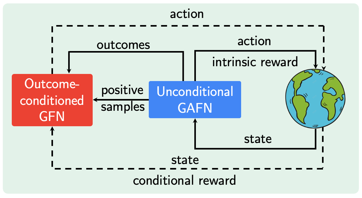
Figure 1: The unsupervised pre-training phase of outcome-conditioned GFlowNet.

4.1 Unsupervised Pre-Training Stage

As GFlowNets are typically learned with a given reward function, it remains an open challenge for how to pre-train them in a reward-free fashion. We propose a novel method for unsupervised pre-training of GFlowNets without task-specific rewards. We formulate the problem of pre-training GFlowNets as a self-supervised problem of learning an outcome-conditioned GFlowNet (OC-GFN) which learns to reach any input target outcomes, inspired by the success of goal-conditioned reinforcement learning in generalizing to a variety of tasks when it is tasked with different goals (Fang et al., 2022). We denote the outcome as $y=f(s)$, where $f$ is an identity function and $s$ is a terminal state, so the space of outcomes is the same as the state space $\mathcal{X}$. What makes OC-GFN special is that, when fully trained, given a reward $R$ a posterior as a function $r$ of the outcome, i.e., $R(s)=r(y)$, one can adapt the OC-GFN to sample from this reward, which can generalize to tasks with different rewards.

Algorithm 1 Reward-free Pre-training of Unsupervised GFlowNets.

0:  GAFlowNet $F^{U}(s),P_{F}^{U}(s^{\prime}|s),P_{B}^{U}(s|s^{\prime})$; fixed target network $\bar{\phi}$; predictor network $\phi$; Outcome-conditioned GFlowNet (OC-GFN) $F^{C}(s|y),P_{F}^{C}(s^{\prime}|s,y),P_{B}^{C}(s|s^{\prime},y)$

1:  for each training step $t=1$ to $T$ do

2:     Collect a trajectory $\tau^{+}=\{s_{0}^{+}\to\dots\to s_{n}^{+}\}$ with $P_{F}^{U}$

3:     // Update the outcome-conditioned GFlowNet model

4:     $y^{+}\leftarrow f(s^{+})$, $R(s_{n}^{+}|y^{+})\leftarrow\mathbbm{1}\{{f(s^{+}_{n})=y^{+}}\}\equiv 1$

5:     Update OC-GFN towards minimizing Eq. (5) with $\tau^{+}$ and $R(s_{n}^{+}|y^{+})$

6:     Collect a trajectory $\tau^{-}=\{s_{0}^{-}\to\dots\to s_{n}^{-}\}$ with $P_{F}^{C}$ conditioned on $y^{+}$

7:     $y^{-}\leftarrow f(s^{-})$, $R(s_{n}^{-}|y^{+})\leftarrow\mathbbm{1}\{{f(s^{-}_{n})=y^{+}}\}$

8:     Update OC-GFN towards minimizing Eq. (5) with $\tau^{-}$ and $R(s_{n}^{-}|y^{+})$

9:     // Update the unconditional GAFlowNet model

10:     Update GAFlowNet towards optimizing Eq. (2) based on $\tau^{+}$ and $r_{i}\leftarrow||\bar{\phi}(s)-\phi(s)||_{2}$

11:     Update the predictor network $\phi$ towards minimizing $||\bar{\phi}(s)-\phi(s)||_{2}$

4.1.1 Outcome-Conditioned GFlowNets (OC-GFN)

We extend the idea of flow functions and policies in GFlowNets to OC-GFN that can generalize to different outcomes $y$ in the outcome space, which is trained to achieve specified $y$. OC-GFN can be realized by providing an additional input $y$ to the flows and policies, resulting in outcome-conditioned forward and backward policies $P_{F}(s^{\prime}|s,y)$ and $P_{B}(s|s^{\prime},y)$, and flows $F(s|y)$. The resulting learning objective for OC-GFN for intermediate states is shown in Eq. (3).

$$F(s|y)P_{F}(s^{\prime}|s,y)=F(s^{\prime}|y)P_{B}(s|s^{\prime},y).$$ (3)

Outcome generation

We can train OC-GFN by conditioning outcomes-conditioned flows and policies on a specified outcome $y$, and we study how to generate them autotelicly. It is worth noting that we need to train it with full-support over $y$. We propose to leverage GAFN (Pan et al., 2023b) with the introduction of augmented flows that enable efficient reward-free exploration purely by intrinsic motivation (Burda et al., 2018). In practice, we generate diverse outcomes $y$ with GAFN, and provide them to OC-GFN to sample an outcome-conditioned trajectory $\tau=(s_{0},\cdots,s_{n})$. The resulting conditional reward is given as ${R}(s_{n}|y)=\mathbbm{1}\{{f(s_{n})=y}\}$. Therefore, OC-GFN receives a zero reward if it fails to reach the target outcome, and a positive reward otherwise, which results in learning an outcome achieving policy.

Contrastive training

However, it can be challenging to efficiently train OC-GFN in problems with large outcome spaces. This is because it can be hard to actually achieve the outcome and obtain a meaningful learning signal owing to the sparse nature of the rewards — most of the conditional rewards $R(s_{n}|y)$ will be zero if $f(s_{n})\neq y$ when OC-GFN fails to reach the target.

To alleviate this we propose a contrastive learning objective for training the OC-GFN. After sampling a trajectory $\tau^{+}=\{s_{0}^{+}\to\cdots\to s_{n}^{+}\}$ from unconditional GAFN, we first train an OC-GFN based on this off-policy trajectory by assuming it has the ability to achieve $y^{+}=s_{n}^{+}$ when conditioned on $y^{+}$. Note that the resulting conditional reward $R(s_{n}^{+}|y^{+})=\mathbbm{1}\{{f(s^{+}_{n})=y^{+}}\}\equiv 1$ in this case, as all correspond to successful experiences that provide meaningful learning signals to OC-GFN. We then sample another on-policy trajectory $\tau^{-}=\{s_{0}^{-}\to\cdots\to s_{n}^{-}\}$ from OC-GFN by conditioning it on $y^{+}$, and evaluate the conditional reward by $R(s_{n}^{-}|y^{+})=\mathbbm{1}\{{f(s^{-}_{n})=y^{+}}\}$. Although most of $R(s_{n}^{-}|y^{+})$ can be zero in large outcome spaces during early learning, we provide sufficient successful experiences in the initial phase, which is also related to goal relabeling (Andrychowicz et al., 2017). This can be viewed as an implicit curriculum for improving the training of OC-GFN.

Outcome teleportation

The contrastive training paradigm can significantly improve learning efficiency by providing a bunch of successful trajectories with meaningful learning signals, which tackles the particular challenge of sparse rewards during learning. However, the agent may still suffer from poor learning efficiency in long-horizon tasks, as it cannot effectively propagate the success/failure signal back to each step. We propose a novel technique, outcome teleportation, for further improving the learning efficiency of OC-GFN as in Eq. (4), which considers the terminal reward $R(x|y)$ for every transition.

$$F(s|y)P_{F}(s^{\prime}|s,y)=F(s^{\prime}|y)P_{B}(s|s^{\prime},y)R(x|y).$$ (4)

This formulation can efficiently propagate the guidance signal to each transition in the trajectory, which can significantly improve learning efficiency, particularly in high-dimensional outcome spaces, as investigated in Section 5.2. It can be interpreted as a form of reward decomposition in outcome-conditioned tasks with binary rewards. In practice, we train OC-GFN by minimizing the following loss function ${\mathcal{L}}_{{\text{O}C-GFN}}(\tau,y)$ in log-scale obtained from Eq. (5), i.e.,

$$\sum_{s\to s^{\prime}\in\tau}\left(\log F(s|y)+\log P_{F}(s^{\prime}|s,y)-\log F(s^{\prime}|y)-\log P_{B}(s|s^{\prime},y)-\log R(x|y)\right)^{2}.$$ (5)

Theoretical justification. We now justify that when OC-GFN is trained to completion, it can successfully reach any specified outcome. The proof can be found in Appendix A.1.

Proposition 4.1.

If $\mathcal{L}_{{\text{O}C-GFN}}(\tau,y)=0$ for all trajectories $\tau$ and outcomes $y$, then the outcome-conditioned forward policy $P_{F}(s^{\prime}|s,y)$ can successfully reach the target outcome $y$.

The resulting procedure for the reward-free unsupervised pre-training of OC-GFN is summarized in Algorithm 1 and illustrated Figure 1.

4.2 Supervised Fine-Tuning Stage

In this section, we study how to leverage the pre-trained OC-GFN model and adapt it for downstream tasks with new reward functions.

A remarkable aspect of GFlowNets is the ability to demonstrate the reasoning potential in generating a task-specific policy. By utilizing the pre-trained OC-GFN model with outcome-conditioned flows $F(s|y)$ and policies $P_{F}(s^{\prime}|s,y)$, we can directly obtain a policy that samples according to a new task-specific reward function $R(s)=r(y)$ according to Eq. (6), which is based on (Bengio et al., 2023). A detailed analysis for this can be found in Appendix A.2.

$$P_{F}^{r}(s^{\prime}|s)=\frac{\sum_{y}r(y)F(s|y)P_{F}(s^{\prime}|s,y)}{\sum_{y}r(y)F(s|y)}$$ (6)

Eq. (6) serves as the foundation for converting a pre-trained OC-GFN model to handle downstream tasks with new and even out-of-distribution rewards. Intriguingly, this conversion can be achieved without any re-training for OC-GFN on downstream tasks. This sets it apart from the typical fine-tuning process in reinforcement learning, which typically requires re-training to adapt a policy, since they generally learn reward-maximizing policies that may discard valuable information.

Directly estimating the above summation often necessitates the use of Monte-Carlo averaging for making each decision. Yet, this can be computationally expensive in high-dimensional outcome spaces if we need to calculate this marginalization at each decision-making step, which leads to slow thinking. To improve its efficiency in complex scenarios, it is essential to develop strategies that are both efficient while maintaining accurate estimations.

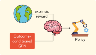
(a)

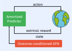
(b)

Figure 2: Left: Convert the outcome-conditioned GFlowNet to downstream tasks without re-training the networks. Right: An efficient amortized predictor in the supervised fine-tuning phase.

Algorithm 2 Supervised Fine-Tuning of Outcome-Conditioned GFlowNets.

1:  Initialize the numerator network $N(s^{\prime}|s)$ and the GFlowNet-like predictor network $Q(y|s^{\prime},s)$

2:  Obtain the pre-trained outcome-conditioned state $F(s|y)$ and forward policy $P_{F}(s^{\prime}|s,y)$

3:  for each training step $t=1$ to $T$ do

4:     Collect a trajectory $\tau=\{s_{0}\to\cdots s_{n}\}$ with $N(s^{\prime}|s)$

5:     Sample outcomes $y$ from a tempered/$\epsilon$-greedy version of $Q(\cdot|s^{\prime},s)$

6:     Update $N$ and $Q$ towards minimizing Eq. (9)

7:  Compute the policy $P_{F}^{r}(s^{\prime}|s)={N(s^{\prime}|s)}/{\sum_{s^{\prime}}N(s^{\prime}|s)}$

Learning an Amortized Predictor

In this section, we propose a novel approach to approximate this marginal by learning an amortized predictor.

Concretely, we propose to estimate the intractable sums in the numerator in Eq. (6) by a numerator network $N(s^{\prime}|s)\approx\sum_{y}r(y)F(s|y)P_{F}(s^{\prime}|s,y)$. This would allow us to efficiently estimate the intractable sum with the help of $N(s^{\prime}|s)$ that directly estimates $N(\cdot|s)$ for any state $s$, which could benefit from the generalizable structure of outcomes with neural networks. We can also obtain the corresponding policy by $P_{F}^{r}(s^{\prime}|s)=\frac{N(s^{\prime}|s)}{\sum_{s^{\prime}}N(s^{\prime}|s)}$. For learning the numerator network $N(\cdot|s)$, we need to have a sampling policy for sampling outcomes $y$ given states $s$ and next states $s^{\prime}$, which can be achieved by

$$Q(y|s^{\prime},s)=\frac{r(y)F(s|y)P_{F}(s^{\prime}|s,y)}{N(s^{\prime}|s)}.$$ (7)

Therefore, we have the following constraint according to Eq. (7)

$$N(s^{\prime}|s)Q(y|s^{\prime},s)=r(y)F(s|y)P_{F}(s^{\prime}|s,y),$$ (8)

based on which we derive the corresponding loss function by minimizing their difference by training in the log domain, i.e.,

$$\mathcal{L}_{\text{a}mortized}=\left(\log N(s^{\prime}|s)+\log Q(y|s^{\prime},s)-\log r(y)-\log F(s|y)-\log P_{F}(s^{\prime}|s,y)\right)^{2}.$$ (9)

Theoretical justification. In Proposition 4.2, we show that $N(s^{\prime}|s)$ can correctly estimate the summation when it is trained to completion and the distribution of outcomes $y$ has full support.

Proposition 4.2.

Suppose that $\forall(s,s^{\prime},y)$, $\mathcal{L}_{\text{a}mortized}(s,s^{\prime},y)=0$, then the amortized predictor $N(s^{\prime}|s)$ estimates $\sum_{y}r(y)F(s|y)P_{F}(s^{\prime}|s,y)$.

The proof can be found in Appendix A.3. Proposition 4.2 justifies the use of the numerator network as an efficient alternative for estimating the computationally intractable summation in Eq. (6).

Empirical validation. We now investigate the converted/learned sampling policy in the standard GridWorld domain (Bengio et al., 2021), which has a multi-modal reward function. More details about the setup is in Appendix B.1 due to space limitation. We visualize the last $2\times 10^{5}$ samples from different baselines including training GFN from scratch, OC-GFN with the Monte Carlo-based estimation with Eq. (6) and the amortized marginalization approach with Eq. (9).

As shown in Figure 3(b), directly training GFN with trajectory balance (Malkin et al., 2022) can suffer from the mode collapse problem and fail to discover all modes of the target distribution in Figure 3(a). On the contrary, we can directly obtain a policy from the pre-trained OC-GFN model that samples proportionally to the target rewards as shown in Figure 3(c), while fine-tuning OC-GFN with the amortized inference could also match the target distribution as in Figure 3(d), which validates its effectiveness in estimating the marginal.

(a)

(b)

(c)

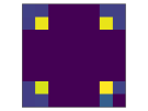
(d)

Figure 3: Distribution of $2\times 10^{5}$ samples from different baselines. (a) Target distribution. (b) GFN (from scratch). (c) OC-GFN (Monte Carlo-based). (d) OC-GFN (Amortizer-based).

Practical implementation. In practice, we can train the amortized predictor $N(\cdot|s)$ and the sampling policy $Q(\cdot|s^{\prime},s)$ in a GFlowNet-like procedure. We sample $(s,s^{\prime})$ with $N$ by interacting with the environment. This can also be realized by sampling from the large and diverse dataset $\mathcal{D}$ obtained in the pre-training stage. We then sample outcomes $y$ from the sampling policy $Q(\cdot|s^{\prime},s)$, which can incorporate its tempered version or with $\epsilon$-greedy exploration (Bengio et al., 2021) for obtaining rich distributions of $y$. We can then learn the amortized predictor and the sampling policy by one of these sampled experiences. Finally, we can derive the policy that will be converted to downstream tasks by $P_{F}^{r}(s^{\prime}|s)={N(s^{\prime}|s)}/{\sum_{s^{\prime}}N(s^{\prime}|s)}$. The resulting training algorithm is summarized in Algorithm 2 and the right part in Figure 2.

5 Experiments

In this section, we conduct extensive experiments to better understand the effectiveness of our approach and aim to answer the following key questions: (i) How do outcome-conditioned GFlowNets (OC-GFN) perform in the reward-free unsupervised pre-training stage? (ii) What is the effect of key modules? (iii) Can OC-GFN transfer to downstream tasks efficiently? (iv) Can they scale to complex and practical scenarios like biological sequence design?

5.1 GridWorld

We first conduct a series of experiments on GridWorld (Bengio et al., 2021) to understand the effectiveness of the proposed approach. In the reward-free unsupervised pre-training phase, we train a (unconditional) GAFN (Pan et al., 2023b) and an outcome-conditioned GFN (OC-GFN) on a map without task-specific rewards, where GAFN is trained purely from self-supervised intrinsic rewards according to Algorithm 1. We investigate how well OC-GFN learns in the unsupervised pre-training stage, while the supervised fine-tuning stage has been discussed in Section 4.2. Each algorithm is run for $3$ different seeds and the mean and standard deviation are reported. A detailed description of the setup and hyperparameters can be found in Appendix B.1.

Outcome distribution. We first evaluate the quality of the exploratory data collected by GAFN, as it is essential for training OC-GFN with a rich distribution of outcomes. We demonstrate the sample distribution from GAFN in Figure 4(a), which has great diversity and coverage, and validates its effectiveness in collecting unlabeled exploratory trajectories for providing diverse target outcomes for OC-GFN to learn from.

(a)

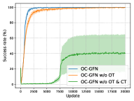
(b)

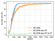
(c)

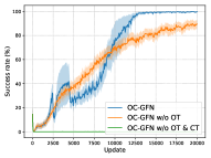
(d)

Figure 4: Results in GridWorld in different with different scales of the task. (a) Outcome distribution. (b)-(d) Success rate of OC-GFN and its variants in small, medium, and large maps, respectively.

Outcome reaching performance. We then investigate the key designs in pre-training OC-GFN by analyzing its success rate for achieving target outcomes. We also ablate key components to investigate the effect of contrastive training (CT) and outcome teleportation (OT). The success rates of OC-GFN and its variants are summarized in Figures 4(b)-(d) in different sizes of the map from small to large. As shown, OC-GFN can successfully learn to reach specified outcomes with a success rate of nearly $100\%$ at the end of training in maps with different sizes. Disabling the outcome teleportation component (OC-GFN w/o OT) leads to lower sample efficiency, in particular in larger maps. Further deactivating the contrastive training process (OC-GFN w/o OT & CT) fails to learn well as the size of the outcome space grows, since the agent can hardly collect successful trajectories for meaningful updates. This indicates that both contrastive training and outcome teleportation are important for successfully training OC-GFN in large outcome spaces. It is also worth noting that outcome teleportation can significantly boost learning efficiency in problems with a combinatorial explosion of outcome spaces (e.g., sequence generation in the following sections).

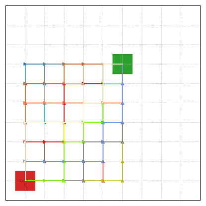
(a)

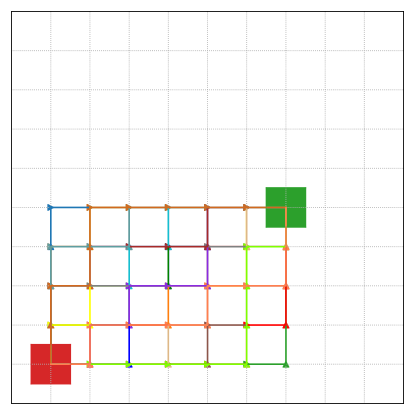
(b)

Figure 5: Visualization of the behaviors of OC-GFN.

Outcome-conditioned behaviors. We now visualize the learned behaviors of OC-GFN in Figure 5, where the red and green squares denote the starting point and the goal, respectively. We find that OC-GFN can not only reach different specified outcomes with a high success rate, but also discover diverse trajectories leading to a specified outcome $y$ with the forward policy $P_{F}$. OC-GFN is able to generate diverse trajectories, which is different from typical goal-conditioned reinforcement learning approaches (Schaul et al., 2015) that usually only learn a single solution to the goal state. This ability can be very helpful for generalizing to downstream tasks with similar structure but subtle changes (e.g., obstacles in the maze) (Kumar et al., 2020).

5.2 Bit Sequence Generation

We study the bit sequence generation task (Malkin et al., 2022), where the agent generates sequences of length $n$ in a left-to-right manner. At each time step, the agent appends a $k$-bit “word" from a vocabulary $V$ to the current state. We follow the same procedure for pre-training OC-GFN without task-specific rewards as in Section 5.1 with more details in Appendix B.1.

Analysis of the unsupervised pre-training stage. We first analyze how well OC-GFN learns in the unsupervised pre-training stage by investigating its success rate for achieving specified outcomes in bit sequence generation problems with different scales including small, medium, and large. As shown in Figures 6(a)-(c), OC-GFN can successfully reach outcomes, leading to a high success rate as summarized in Figure 6(d). It is also worth noting that it fails to learn when the outcome teleportation module is disabled due to the particularly large outcome spaces. In such highly challenging scenarios, the contrastive training paradigm alone does not lead to efficient learning.

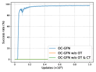
(a) Small.

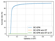
(b) Medium.

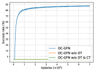
(c) Large.

Size   Success rate
Small	$98.37\pm 0.33$%
Medium	$97.22\pm 1.70$%
Large	$93.75\pm 2.04$%

(d) Summary.

Figure 6: Success rates in the bit sequence generation task with different scales of the task.

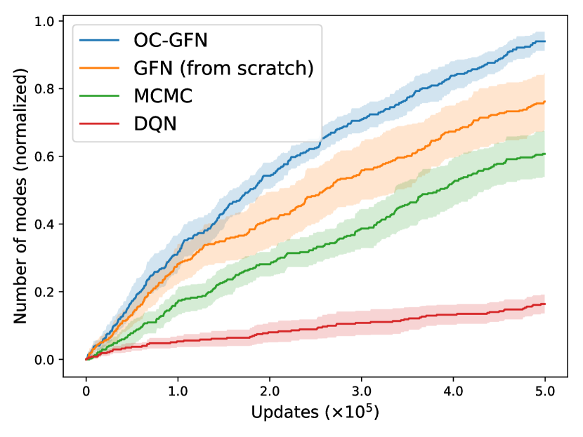
Figure 7: Results in bit sequence generation.

Analysis of the Supervised Fine-Tuning Stage. After we justified the effectiveness of training OC-GFN in the unsupervised pre-training stage, we study whether fine-tuning the model with the amortized approach can enable faster mode discovery when adapting to downstream tasks (as described in Appendix B.1). We compare the proposed approach against strong baselines including training a GFN from scratch (Bengio et al., 2023), Metropolis-Hastings-MCMC (Dai et al., 2020), and Deep Q-Networks (DQN) (Mnih et al., 2015). We evaluate each method in terms of the number of modes discovered during the course of training as in previous works (Malkin et al., 2022). We summarize the normalized (between $0$ and $1$ to facilitate comparison across tasks) number of modes averaged over each downstream task in Figure 7, while results for each individual downstream task can be found in Appendix B.2 due to space limitation.

We find that OC-GFN significantly outperforms baselines in mode discovery in both efficiency and performance, while DQN gets stuck and does not discover diverse modes due to the reward-maximizing nature, and MCMC fails to perform well in problems with larger state spaces.

5.3 TF Bind Generation

We study a more practical task of generating DNA sequences with high binding activity with targeted transcription factors (Jain et al., 2022). The agent appends a symbol from the vocabulary to the current state (a partially constructed sequence) at each step. We consider $30$ different downstream tasks studied in (Barrera et al., 2016), which conducted biological experiments to determine the binding properties between a range of transcription factors and every conceivable DNA sequence.

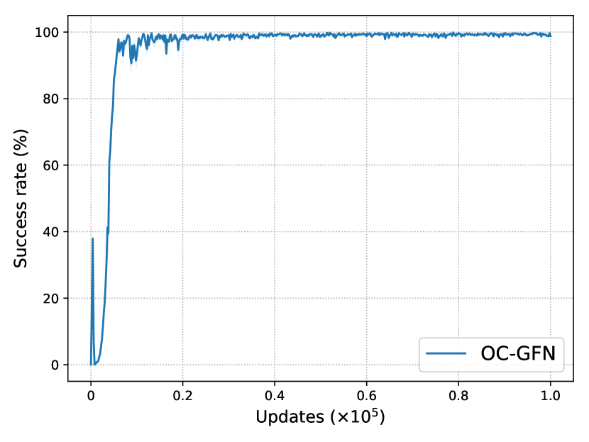
(a)

Figure 8: The success rate of OC-GFN in TF Bind generation.

Analysis of the unsupervised pre-training stage. We analyze how well OC-GFN learns by evaluating its success rate. Figure 8 shows that OC-GFN can successfully achieve the targeted goals with a success rate of nearly $100\%$ in the practical task of generating DNA sequences.

Analysis of the supervised fine-tuning stage. We investigate how well OC-GFN can transfer to downstream tasks for generating TF Bind 8 sequences. We tune the hyperparameters on the task PAX3_R270C_R1, and evaluate the baselines on the other $29$ downstream tasks. We investigate the learning efficiency and performance in terms of the number of modes and the top-$K$ scores during the course of training. The results in $2$ downstream tasks are shown in Figure 9, with the full results in Appendix B.3 due to space limitation. Figures 9(a)-(b) illustrate the number of discovered modes while Figures 9(c)-(d) shows the top-$K$ scores. We find that the proposed approach discovers more diverse modes faster and achieves higher top-$K$ ($K=100$) scores compared to baselines. We summarize the rank of each baseline in all $30$ downstream tasks (Zhang et al., 2021) in Appendix B.3, where OC-GFN ranks highest compared with other methods. We further visualize in Figure 9(e) the t-SNE plots of the TF Bind 8 sequences discovered by transferring OC-GFN with the amortized approach and the more expensive but competitive training of a GFN from scratch. As shown, training a GFN from scratch only focuses on limited regions while the OC-GFN has a greater coverage.

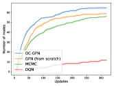
(a)

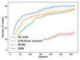
(b)

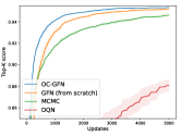
(c)

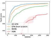
(d)

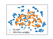
(e)

Figure 9: Results in the TF Bind sequence generation task in different downstream tasks.

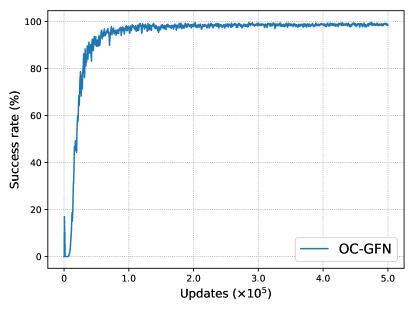
(a)

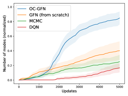
(b)

Figure 10: Results in RNA generation. Left: success rate. Right: number of modes (normalized).

5.4 RNA Generation

We study the performance of the proposed method in a larger task of generating RNA sequences that bind to a given target introduced in (Lorenz et al., 2011). We follow the same procedure as in Section 5.3, with additional details provided in Appendix B.1. We consider four different downstream tasks from ViennaRNA (Lorenz et al., 2011), each considering the binding energy with a different target as a reward.

The left part in Figure 10 shows that OC-GFN achieves a success rate of almost $100\%$ at the end of the pre-training stage. The right part in Figure 10 summarizes the averaged normalized (between $0$ and $1$ to facilitate comparison across tasks) performance in terms of the number of modes averaged over four downstream tasks, where the performance for each individual task is shown in Appendix B.4. We observe that OC-GFN is able to achieve much higher diversity than baselines, indicating that the pre-training phase enables the OC-GFN to explore the state space much more efficiently.

5.5 Antimicrobial Peptide Generation

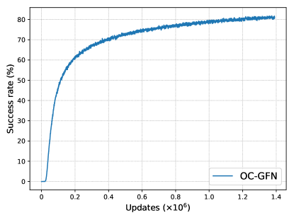
(a) Success rate.

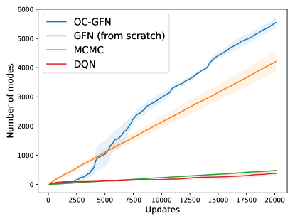
(b) Number of modes.

Figure 11: Results in AMP generation.

To demonstrate the scalability of our approach to even more challenging and complex scenarios, we also evaluate it on the biological task of generating antimicrobial peptides (AMP) with lengths $50$ (Jain et al., 2022) (resulting in an outcome space of $20^{50}$ candidates).

Figure 11(a) demonstrates the success rate of OC-GFN for achieving target outcomes, which can still reach a high success rate in particularly large outcome spaces with our novel training paradigm according to contrastive learning and fast goal propagation. Figure 11(b) shows the number of modes discovered, where OC-GFN provides consistent improvements, which validates the efficacy of OC-GFN to successfully scale to much larger-scale tasks.

6 Conclusion

In this paper, we propose a novel method for unsupervised pre-training of GFlowNets through an outcome-conditioned GFlowNet, coupled with a new approach to efficiently fine-tune the pre-trained model for downstream tasks. Our work opens the door for GFlowNets to be pre-trained for fine-tuning for downstream tasks by leveraging learned shared structure. Empirical results on the standard GridWorld domain validate the effectiveness of the proposed approach in successfully achieving targeted outcomes and the efficiency of the amortized predictor. We also conduct extensive experiments in the more complex and challenging biological sequence design tasks to demonstrate its practical scalability. The proposed method greatly improves learning performance compared with strong baselines including training a GFlowNet from scratch, particularly in tasks which are challenging for GFlowNets to learn.

Appendix A Proofs

A.1 Proof of Proposition 4.1

Proposition 4.1 If $\mathcal{L}_{\text{OC-GFN}}(\tau,y)=0$ for all trajectories $\tau$ and outcomes $y$, then the outcome-conditioned forward policy $P_{F}(s^{\prime}|s,y)$ can successfully reach any target outcome $y$.

Proof.

As $\mathcal{L}_{\text{OC-GFN}}(\tau,y)=0$ is satisfied for all trajectories $\tau=\{s_{0},\cdots,s_{n}=x\}$ and outcomes $y$, we have that

$$F(s_{0}|y)\prod_{t=0}^{n-1}P_{F}(s_{t+1}|s_{t},y)=\prod_{t=0}^{n-1}R(x|y)P_{B}(s_{t+1}|s_{t},y).$$ (10)

Since $R(x|y)$ is either $1$ or $0$ in outcome-condition tasks, we get that

$$F(s_{0}|y)\prod_{t=0}^{n-1}P_{F}(s_{t+1}|s_{t},y)=R(x|y)\prod_{t=0}^{n-1}P_{B}(s_{t+1}|s_{t},y).$$ (11)

Then, the probability of reaching the target outcome $y$ is

$$P(x=y|y)=\sum_{\tau,s_{n}=y}P(\tau|y).$$ (12)

By definition, we have that

$$P(\tau|y)=\prod_{t=0}^{n-1}P_{F}(s_{t+1}|s_{t},y).$$ (13)

Therefore, we get that

$$P(x=y|y)=\sum_{\tau,s_{n}=y}\prod_{t=0}^{n-1}P_{F}(s_{t+1}|s_{t},y).$$ (14)

Combing Eq. (11) with Eq. (13), and due to the law of total probability, we obtain that

$$F(s_{0}|y)P(x=y|y)=\sum_{\tau,s_{n}=y}\prod_{t=0}^{n-1}P_{B}(s_{t+1}|s_{t},y)=1.$$ (15)

With the same analysis for the case where the agent fails to reach the target outcome $y$, i.e., $x\neq y$, we have that

$$\forall x\neq y,\quad F(s_{0}|y)P(x|y)=0.$$ (16)

Combing Eq. (15) with Eq. (16), we have that $P(x=y|y)=1$, i.e., the outcome-conditioned forward policy $P_{F}(s^{\prime}|s,y)$ can successfully reach any target outcome $y$.

∎

A.2 Analysis of the Conversion Policy

We now elaborate on more details about the effect of Eq. (6) in the text based on (Bengio et al., 2023).

When the outcome-conditioned GFlowNet (OC-GFN) is trained to completion, the following flow consistency constraint in the edge level is satisfied for intermediate states.

$$F(s|y)P_{F}(s^{\prime}|s,y)=F(s^{\prime}|y)P_{B}(s|s^{\prime},y)$$ (17)

We define the state flow function as $F^{r}(s)=\sum_{y}r(y)F(s|y)$, and the backward policy as

$$P_{B}^{r}(s|s^{\prime})=\frac{\sum_{y}r(y)F(s^{\prime}|y)P_{B}(s|s^{\prime},y)}{\sum_{y}r(y)F(s^{\prime}|y)},$$ (18)

while the forward policy is defined in Eq. (6), i.e.,

$$P_{F}^{r}(s^{\prime}|s)=\frac{\sum_{y}r(y)F(s|y)P_{F}(s^{\prime}|s,y)}{\sum_{y}r(y)F(s|y)}$$ (19)

Then, we have

$$F^{r}(s)P_{F}^{r}(s^{\prime}|s)=\sum_{y}r(y)F(s|y)P_{F}(s^{\prime}|s,y),$$ (20)

and

$$F^{r}(s^{\prime})P_{B}^{r}(s|s^{\prime})=\sum_{y}r(y)F(s^{\prime}|y)P_{B}(s|s^{\prime},y).$$ (21)

Combining the above equations, we have that

$$F^{r}(s)P_{F}^{r}(s^{\prime}|s)=F(s^{\prime})^{r}P_{B}^{r}(s|s^{\prime}),$$ (22)

which corresponds to a new flow consistency constraint in the edge level. A more detailed proof can be found in (Bengio et al., 2023).

Discussion about applicability

It is also worth noting that OC-GFN should be built upon the detailed balance objective (Bengio et al., 2023) discussed in Section 2 or other variants which learn flows (e.g., sub-trajectory balance (Madan et al., 2022), flow matching (Bengio et al., 2021)). Instead, the trajectory balance objective (Malkin et al., 2022), does not learn a state flow function necessary for converting the pre-trained OC-GFN model to the new policy $\pi_{r}$.

A.3 Proof of Proposition 4.2

Proposition 4.2 Suppose that $\forall(s,s^{\prime},y)$, $\mathcal{L}_{\text{a}mortized}(s,s^{\prime},y)=0$, then the amortized predictor $N(s^{\prime}|s)$ estimates $\sum_{y}r(y)F(s|y)P_{F}(s^{\prime}|s,y)$.

Proof.

As $\mathcal{L}_{\text{amortized}}(s,s^{\prime},y)=0$ for all states $s$, next states $s^{\prime}$, and outcomes $y$, we have that

$$\forall s,s^{\prime},y,\quad N(s^{\prime}|s)Q(y|s^{\prime},s)=r(y)F(s|y)P_{F}(s^{\prime}|s,y).$$ (23)

Therefore, by summing over all possible outcomes $y$ on both sides, we obtain that

$$\forall s,s^{\prime},\quad\sum_{y}N(s^{\prime}|s)Q(y|s^{\prime},s)=\sum_{y}r(y)F(s|y)P_{F}(s^{\prime}|s,y).$$ (24)

As $\sum_{y}Q(y|s^{\prime},s)=1$, we get that

$$\forall s,s^{\prime},\quad N(s^{\prime}|s)=\sum_{y}r(y)F(s|y)P_{F}(s^{\prime}|s,y).$$ (25)

Based on the above analysis, we get that the amortized predictor $N(s^{\prime}|s)$ estimates the marginal $\sum_{y}r(y)F(s|y)P_{F}(s^{\prime}|s,y)$.

∎

Appendix B Experimental Details

All baseline methods are implemented based on the open-source implementation, where we follow the default hyperparameters and setup as in (Bengio et al., 2021). The code will be released upon publication of the paper.

B.1 Experimental Setup

GridWorld

We employ the same standard reward function for GridWorld from (Bengio et al., 2021) as in Eq. (26), where the target reward distribution is shown in Figure 3(a) with $4$ modes located near the corners of the maze.

$$R(x)=\frac{1}{2}\prod_{i}\mathbb{I}\left(0.25<\left|x_{i}/H-0.5\right|\right)+2\prod_{i}\mathbb{I}\left(0.3<\left|x_{i}/H-0.5\right|<0.4\right)+10^{-6}.$$ (26)

The GFlowNet model is a feedforward network consisting of two hidden layers with $256$ hidden units per layer using LeakyReLU activation. We use a same network structure for the outcome-conditioned GFlowNet model, except that we concatenate the state and outcome as input to the network. For the unconditional GAFlowNet model, we follow (Pan et al., 2023b) and leverage random network distillation as the intrinsic reward mechanism. The coefficient for intrinsic rewards is set to be $1.0$ (which purely learns from intrinsic motivation without task-specific rewards). We also use a same network structure for the amortized predictor network. We train all models with the Adam (Kingma and Ba, 2015) optimizer (learning rate is $0.001$) based on samples from a parallel of $16$ rollouts in the environment.

Bit Sequence Generation

We consider generating bit sequences with fixed lengths based on (Malkin et al., 2022). The GFlowNet model is a feedforward network that consists of $2$ hidden layers with $2048$ hidden units with ReLU activation. The exploration strategy is $\epsilon$-greedy with $\epsilon=0.0005$, while we set the sampling temperature to $1.0$, and use a reward exponent of $3$. The learning rate for training the GFlowNet model is $5\times 10^{-3}$ with the Adam optimizer, with a batch size of $16$. We use a same network structure for the outcome-conditioned GFlowNet model and the amortized predictor network. We train all models for $50000$ iterations, using a parallel of $16$ rollouts in the environment.

TF Bind and RNA Generation

For the TFBind-8 generation task, we follow the same setup as in (Jain et al., 2022). The vocabulary consists of $4$ nucleobases, and the trajectory length is $8$ and $14$. The GFlowNet model is a feedforward network that consists of $2$ hidden layers with $2048$ hidden units and ReLU activation. The exploration strategy is $\epsilon$-greedy with $\epsilon=0.001$, while the reward exponent is $3$. The learning rate for training the GFlowNet model is $1e-4$, with a batch size of $32$. We train all models for $5000$ iterations.

AMP Generation

We basically follow the same setup for the antimicrobial peptide generation task as in Malkin et al. (2022), Jain et al. (2022), where we consider generating AMP sequence with length $50$. The GFlowNet model is an MLP that consists of $2048$ hidden layers with $2$ hidden units with ReLU activation. The exploration strategy is $\epsilon$-greedy with $\epsilon=0.01$, while the sampling temperature is set to $1$, and uses a reward exponent of $3$. The lr for training the GFlowNet model is $0.001$, and the batch size is $16$.

B.2 Additional Results on the Bit Sequence Generation Task

As shown in Figures 12(a)-(c), OC-GFN is more efficient at discovering modes and discovers more modes, compared with baselines in different scales of the task, from small to large. DQN gets stuck and does not discover diverse modes due to the reward-maximizing nature of regular reinforcement learning algorithms, while MCMC fails to perform well in problems with larger state spaces. Besides different scales of the problem, we also consider different downstream tasks as in Figures 12(d)-(e), which further demonstrate the effectiveness of OC-GFN in the supervised fine-tuning stage.

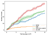
(a)

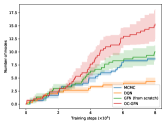
(b)

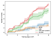
(c)

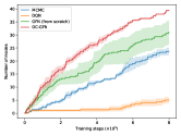
(d)

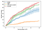
(e)

Figure 12: Results in the bit sequence generation task in different with different scales of the task.

B.3 Additional Results on the TF Bind Generation Task

The full results in the TF Bind generation task are demonstrated in Figure 14 for the $30$ downstream from (Lorenz et al., 2011). The mean rank averaged over all tasks is summarized in Table 1, where OC-GFN significantly outperforms baselines and is able to discover more modes in a more efficient way.

Table 1: Mean rank of each baseline in all downstream tasks (the lower the better).

	DQN	MCMC	GFN (from scratch)	OC-GFN
Number of modes	$4.00$	$2.77$	$1.97$	1.27
Top-$K$ reward	$4.00$	$2.80$	$2.00$	1.20

B.4 Additional Results on the RNA Generation Task

The full results in the RNA sequence generation task are demonstrated in Figure 13 for the four downstream from (Lorenz et al., 2011), where OC-GFN significantly outperforms baseline methods achieving better diversity in a more efficient manner.

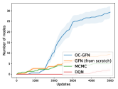
(a)

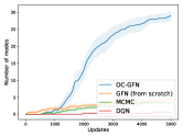
(b)

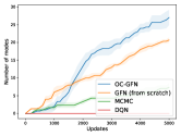
(c)

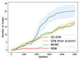
(d)

Figure 13: Full Results in the RNA generation task.

(a)

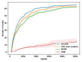
(b)

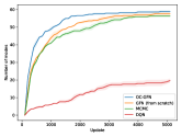
(c)

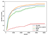
(d)

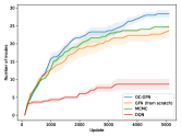
(e)

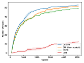
(f)

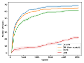
(g)

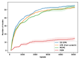
(h)

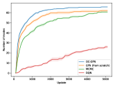
(i)

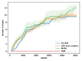
(j)

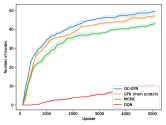
(k)

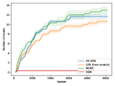
(l)

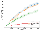
(m)

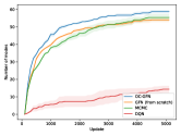
(n)

(o)

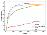
(p)

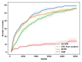
(q)

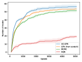
(r)

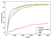
(s)

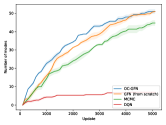
(t)

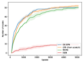
(u)

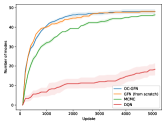
(v)

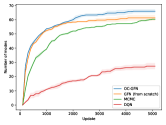
(w)

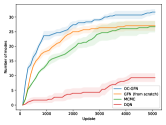
(x)

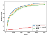
(y)

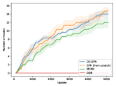
(z)

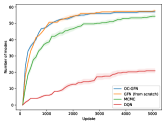
(aa)

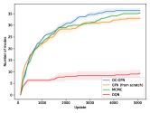
(ab)

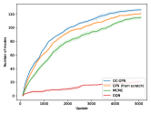
(ac)

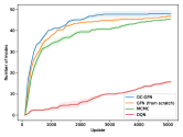
(ad)

Figure 14: Full Results in the TF Bind generation task.

Appendix C Limitations and future directions

We address the potential challenge of sparse rewards in training outcome-conditioned GFlowNet in the unsupervised pre-training stage with a contrastive learning procedure based on the concept of goal relabeing. It is an interesting future direction for considering smoother rewards or other techniques for addressing this problem. In addition, it is also promising to consider continuous outcomes in future works (which has the potential to tackle even larger-scale problems), while our work mainly focuses on discrete outcomes.

References

- Andrychowicz et al. (2017) Marcin Andrychowicz, Filip Wolski, Alex Ray, Jonas Schneider, Rachel Fong, Peter Welinder, Bob McGrew, Josh Tobin, OpenAI Pieter Abbeel, and Wojciech Zaremba. Hindsight experience replay. Advances in neural information processing systems, 30, 2017.
- Barrera et al. (2016) Luis A Barrera, Anastasia Vedenko, Jesse V Kurland, Julia M Rogers, Stephen S Gisselbrecht, Elizabeth J Rossin, Jaie Woodard, Luca Mariani, Kian Hong Kock, Sachi Inukai, et al. Survey of variation in human transcription factors reveals prevalent dna binding changes. Science, 351(6280):1450–1454, 2016.
- Bengio et al. (2021) Emmanuel Bengio, Moksh Jain, Maksym Korablyov, Doina Precup, and Yoshua Bengio. Flow network based generative models for non-iterative diverse candidate generation. Neural Information Processing Systems (NeurIPS), 2021.
- Bengio et al. (2023) Yoshua Bengio, Salem Lahlou, Tristan Deleu, Edward J. Hu, Mo Tiwari, and Emmanuel Bengio. Gflownet foundations. Journal of Machine Learning Research, 24(210):1–55, 2023. URL http://jmlr.org/papers/v24/22-0364.html.
- Brown et al. (2020) Tom Brown, Benjamin Mann, Nick Ryder, Melanie Subbiah, Jared D Kaplan, Prafulla Dhariwal, Arvind Neelakantan, Pranav Shyam, Girish Sastry, Amanda Askell, et al. Language models are few-shot learners. Advances in neural information processing systems, 33:1877–1901, 2020.
- Burda et al. (2018) Yuri Burda, Harrison Edwards, Amos Storkey, and Oleg Klimov. Exploration by random network distillation. arXiv preprint arXiv:1810.12894, 2018.
- Chebotar et al. (2021) Yevgen Chebotar, Karol Hausman, Yao Lu, Ted Xiao, Dmitry Kalashnikov, Jake Varley, Alex Irpan, Benjamin Eysenbach, Ryan Julian, Chelsea Finn, et al. Actionable models: Unsupervised offline reinforcement learning of robotic skills. arXiv preprint arXiv:2104.07749, 2021.
- Dai et al. (2020) Hanjun Dai, Rishabh Singh, Bo Dai, Charles Sutton, and Dale Schuurmans. Learning discrete energy-based models via auxiliary-variable local exploration. Advances in Neural Information Processing Systems, 33:10443–10455, 2020.
- Deleu et al. (2022) Tristan Deleu, António Góis, Chris Emezue, Mansi Rankawat, Simon Lacoste-Julien, Stefan Bauer, and Yoshua Bengio. Bayesian structure learning with generative flow networks. Uncertainty in Artificial Intelligence (UAI), 2022.
- Devlin et al. (2018) Jacob Devlin, Ming-Wei Chang, Kenton Lee, and Kristina Toutanova. Bert: Pre-training of deep bidirectional transformers for language understanding. arXiv preprint arXiv:1810.04805, 2018.
- Eysenbach et al. (2018) Benjamin Eysenbach, Abhishek Gupta, Julian Ibarz, and Sergey Levine. Diversity is all you need: Learning skills without a reward function. International Conference on Learning Representations (ICLR), 2018.
- Eysenbach et al. (2020) Benjamin Eysenbach, Ruslan Salakhutdinov, and Sergey Levine. C-learning: Learning to achieve goals via recursive classification. arXiv preprint arXiv:2011.08909, 2020.
- Fang et al. (2022) Kuan Fang, Patrick Yin, Ashvin Nair, and Sergey Levine. Planning to practice: Efficient online fine-tuning by composing goals in latent space. In 2022 IEEE/RSJ International Conference on Intelligent Robots and Systems (IROS), pages 4076–4083. IEEE, 2022.
- Hansen et al. (2019) Steven Hansen, Will Dabney, Andre Barreto, Tom Van de Wiele, David Warde-Farley, and Volodymyr Mnih. Fast task inference with variational intrinsic successor features. arXiv preprint arXiv:1906.05030, 2019.
- Henaff (2020) Olivier Henaff. Data-efficient image recognition with contrastive predictive coding. In International conference on machine learning, pages 4182–4192. PMLR, 2020.
- Howard and Ruder (2018) Jeremy Howard and Sebastian Ruder. Universal language model fine-tuning for text classification. In Proceedings of the 56th Annual Meeting of the Association for Computational Linguistics (Volume 1: Long Papers), pages 328–339, 2018.
- Hu et al. (2023) Edward J Hu, Nikolay Malkin, Moksh Jain, Katie E Everett, Alexandros Graikos, and Yoshua Bengio. Gflownet-em for learning compositional latent variable models. In International Conference on Machine Learning, pages 13528–13549, 2023.
- Jaderberg et al. (2016) Max Jaderberg, Volodymyr Mnih, Wojciech Marian Czarnecki, Tom Schaul, Joel Z Leibo, David Silver, and Koray Kavukcuoglu. Reinforcement learning with unsupervised auxiliary tasks. In International Conference on Learning Representations, 2016.
- Jain et al. (2022) Moksh Jain, Emmanuel Bengio, Alex Hernandez-Garcia, Jarrid Rector-Brooks, Bonaventure F.P. Dossou, Chanakya Ekbote, Jie Fu, Tianyu Zhang, Micheal Kilgour, Dinghuai Zhang, Lena Simine, Payel Das, and Yoshua Bengio. Biological sequence design with GFlowNets. International Conference on Machine Learning (ICML), 2022.
- Jain et al. (2023a) Moksh Jain, Tristan Deleu, Jason Hartford, Cheng-Hao Liu, Alex Hernandez-Garcia, and Yoshua Bengio. Gflownets for ai-driven scientific discovery. Digital Discovery, 2023a.
- Jain et al. (2023b) Moksh Jain, Sharath Chandra Raparthy, Alex Hernandez-Garcia, Jarrid Rector-Brooks, Yoshua Bengio, Santiago Miret, and Emmanuel Bengio. Multi-objective gflownets. In International Conference on Machine Learning, pages 14631–14653, 2023b.
- Kaelbling (1993) Leslie Pack Kaelbling. Learning to achieve goals. In IJCAI, volume 2, pages 1094–8. Citeseer, 1993.
- Kingma and Ba (2015) Diederik P Kingma and Jimmy Ba. Adam: A method for stochastic optimization. International Conference on Learning Representations (ICLR), 2015.
- Kumar et al. (2020) Saurabh Kumar, Aviral Kumar, Sergey Levine, and Chelsea Finn. One solution is not all you need: Few-shot extrapolation via structured maxent rl. Advances in Neural Information Processing Systems, 33:8198–8210, 2020.
- Lahlou et al. (2023) Salem Lahlou, Tristan Deleu, Pablo Lemos, Dinghuai Zhang, Alexandra Volokhova, Alex Hernández-Garcıa, Léna Néhale Ezzine, Yoshua Bengio, and Nikolay Malkin. A theory of continuous generative flow networks. In International Conference on Machine Learning, pages 18269–18300. PMLR, 2023.
- Liu and Abbeel (2021) Hao Liu and Pieter Abbeel. Aps: Active pretraining with successor features. In International Conference on Machine Learning, pages 6736–6747. PMLR, 2021.
- Lorenz et al. (2011) Ronny Lorenz, Stephan H Bernhart, Christian Höner Zu Siederdissen, Hakim Tafer, Christoph Flamm, Peter F Stadler, and Ivo L Hofacker. ViennaRNA package 2.0. Algorithms for molecular biology, 6(1):26, 2011.
- Madan et al. (2022) Kanika Madan, Jarrid Rector-Brooks, Maksym Korablyov, Emmanuel Bengio, Moksh Jain, Andrei Nica, Tom Bosc, Yoshua Bengio, and Nikolay Malkin. Learning GFlowNets from partial episodes for improved convergence and stability. arXiv preprint 2209.12782, 2022.
- Malkin et al. (2022) Nikolay Malkin, Moksh Jain, Emmanuel Bengio, Chen Sun, and Yoshua Bengio. Trajectory balance: Improved credit assignment in GFlowNets. Neural Information Processing Systems (NeurIPS), 2022.
- Malkin et al. (2023) Nikolay Malkin, Salem Lahlou, Tristan Deleu, Xu Ji, Edward Hu, Katie Everett, Dinghuai Zhang, and Yoshua Bengio. Gflownets and variational inference. International Conference on Learning Representations (ICLR), 2023.
- Mnih et al. (2015) Volodymyr Mnih, Koray Kavukcuoglu, David Silver, Andrei A Rusu, Joel Veness, Marc G Bellemare, Alex Graves, Martin Riedmiller, Andreas K Fidjeland, Georg Ostrovski, et al. Human-level control through deep reinforcement learning. nature, 518(7540):529–533, 2015.
- Nair et al. (2018) Ashvin V Nair, Vitchyr Pong, Murtaza Dalal, Shikhar Bahl, Steven Lin, and Sergey Levine. Visual reinforcement learning with imagined goals. Advances in neural information processing systems, 31, 2018.
- Pan et al. (2023a) Ling Pan, Nikolay Malkin, Dinghuai Zhang, and Yoshua Bengio. Better training of gflownets with local credit and incomplete trajectories. arXiv preprint arXiv:2302.01687, 2023a.
- Pan et al. (2023b) Ling Pan, Dinghuai Zhang, Aaron Courville, Longbo Huang, and Yoshua Bengio. Generative augmented flow networks. International Conference on Learning Representations (ICLR), 2023b.
- Pan et al. (2023c) Ling Pan, Dinghuai Zhang, Moksh Jain, Longbo Huang, and Yoshua Bengio. Stochastic generative flow networks. arXiv preprint arXiv:2302.09465, 2023c.
- Radford et al. (2019) Alec Radford, Jeffrey Wu, Rewon Child, David Luan, Dario Amodei, Ilya Sutskever, et al. Language models are unsupervised multitask learners. OpenAI blog, 1(8):9, 2019.
- Schaul et al. (2015) Tom Schaul, Daniel Horgan, Karol Gregor, and David Silver. Universal value function approximators. In International conference on machine learning, pages 1312–1320. PMLR, 2015.
- Sekar et al. (2020) Ramanan Sekar, Oleh Rybkin, Kostas Daniilidis, Pieter Abbeel, Danijar Hafner, and Deepak Pathak. Planning to explore via self-supervised world models. In International Conference on Machine Learning, pages 8583–8592. PMLR, 2020.
- Sinai et al. (2020) Sam Sinai, Richard Wang, Alexander Whatley, Stewart Slocum, Elina Locane, and Eric Kelsic. Adalead: A simple and robust adaptive greedy search algorithm for sequence design. arXiv preprint, 2020.
- van Krieken et al. (2022) Emile van Krieken, Thiviyan Thanapalasingam, Jakub M Tomczak, Frank van Harmelen, and Annette ten Teije. A-nesi: A scalable approximate method for probabilistic neurosymbolic inference. arXiv preprint arXiv:2212.12393, 2022.
- Veeriah et al. (2018) Vivek Veeriah, Junhyuk Oh, and Satinder Singh. Many-goals reinforcement learning. arXiv preprint arXiv:1806.09605, 2018.
- Zhang et al. (2023a) David W Zhang, Corrado Rainone, Markus Peschl, and Roberto Bondesan. Robust scheduling with gflownets. arXiv preprint arXiv:2302.05446, 2023a.
- Zhang et al. (2021) Dinghuai Zhang, Jie Fu, Yoshua Bengio, and Aaron Courville. Unifying likelihood-free inference with black-box optimization and beyond. arXiv preprint arXiv:2110.03372, 2021.
- Zhang et al. (2023b) Dinghuai Zhang, Hanjun Dai, Nikolay Malkin, Aaron Courville, Yoshua Bengio, and Ling Pan. Let the flows tell: Solving graph combinatorial optimization problems with gflownets. arXiv preprint arXiv:2305.17010, 2023b.
- Zhang et al. (2023c) Dinghuai Zhang, Ling Pan, Ricky TQ Chen, Aaron Courville, and Yoshua Bengio. Distributional gflownets with quantile flows. arXiv preprint arXiv:2302.05793, 2023c.
- Zhao et al. (2021) Rui Zhao, Yang Gao, Pieter Abbeel, Volker Tresp, and Wei Xu. Mutual information state intrinsic control. arXiv preprint arXiv:2103.08107, 2021.
- Zimmermann et al. (2022) Heiko Zimmermann, Fredrik Lindsten, Jan-Willem van de Meent, and Christian A. Naesseth. A variational perspective on generative flow networks. arXiv preprint 2210.07992, 2022.