Hidden Turbulence in van Gogh’s The Starry Night

Abstract

Turbulence or turbulence-like patterns are often depicted in art, such as The Starry Night by Vincent van Gogh. For a long time, it was debated whether the flow in this famous oil painting follows Kolmogorov’s turbulence theory or not. In this work, we show that a Kolmogorov-like spectrum can be obtained if we make the phenomenological assumption that a certain number of "whirls/eddies" are satisfied, which provides a wide range of scales. The scaling range is then expected to extend from the smallest whirls to the largest ones. This results in a $-5/3$ Kolmogorov-like power law in the Fourier power spectrum of the luminance. Additionally, a "$-1$"-like spectrum is observed below the smallest whirls, which can be interpreted in the framework of Batchelor scalar turbulence with a Schmidt number much greater than one. The hidden turbulence is then recovered for The Starry Night.

I Introduction

Turbulence or patterns similar to turbulence are ubiquitous in nature. They are observed not only in nature, such as high Reynolds flows,(Frisch, 1995) active movement of the high concentration of bacteria,(Wensink et al., 2012; Qiu et al., 2016) finance activity,(Mantegna and Stanley, 1996; Schmitt, Schertzer, and Lovejoy, 2000; Li and Huang, 2014) to list a few, but also in arts, such as the famous painting The Yellow River Breaches Its Course attributed to 13th-century Chinese artist Yuan Ma,(Zhou, 2021; Warhaft, 2022), a series draw of water flows by Leonardo da Vinci in 1500s,(Frisch, 1995; Chen, Yang, and Jiang, 2019; Raissi, Yazdani, and Karniadakis, 2020; Marusic and Broomhall, 2021; Colagrossi et al., 2021) The Great Wave off Kanagawa by Hokusai in 1831,(Ornes, 2014) The Starry Night by van Gogh in 1890,(Aragón et al., 2008; Olson, 2014; Beattie and Kriel, 2019; Finlay, 2020) to name a few. For a long time, it was debated whether the flow in van Gogh’s painting satisfies Kolmogorov’s turbulence theory or not.(Aragón et al., 2008; Beattie and Kriel, 2019; Finlay, 2020)

To describe a turbulent flow, Richardson (1922) advocated his cascade picture of the turbulent phenomenon in his seminal work “Weather Prediction by Numerical Process" that

big whirls have little whirls
that feed on their velocity
and little whirls have lesser whirls
and so on to viscosity in the molecule sense

This phenomenological cascading picture has been now widely accepted for describing the kinetic energy (i.e., the square of velocity) qualitatively transferred from large scale structures to small scale ones in turbulent flows, known as the forward energy cascade. Frisch (1995); Alexakis and Biferale (2018); Zhou (2021) Later in 1941, Kolmogorov proposed his famous theory of locally homogeneous and isotropic turbulence to quantitatively characterize the scale-dependent feature of the turbulent flows at high Reynolds number that a scaling range, namely inertial range $k_{L}\ll k\ll k_{\eta}$, has power-law behavior as,

$$E(k)\propto\epsilon^{2/3}k^{-5/3},$$ (1)

where $\epsilon$ is the mean energy dissipation rate per unit; $k$ is the wavenumber, and $k_{\eta}$ and $k_{L}$ are the Kolmogorov and system scales.(Kolmogorov, 1941) This theory, now known as the Kolmogorov 1941 theory of turbulence (K41 for short), is the first theory to provide quantitatively prediction of turbulent flows, and is thus treated as the cornerstone for understanding turbulent flows. (Frisch, 1995; Pope, 2000; Tsinober, 2009; Alexakis and Biferale, 2018) To pursue the Kolmogorov law $-5/3$, several requirements must be satisfied. For example, there should be enough scale separation, which is often quantified by the Reynolds number $\mathrm{Re}=uL/\nu$, where $u$ and $L$ are the characteristic velocity and length scale; $\nu$ is the kinetic viscosity of the fluid. $\mathrm{Re}$ has been interpreted as the ratio between the inertial force and the viscosity force.(Tennekes and Lumley, 1972; Frisch, 1995) Therefore, the velocity scaling behavior has been treated as one of the most important features of high Reynolds number flows.(Frisch, 1995; Tennekes and Lumley, 1972; Tsinober, 2009) The Kolmogorov prediction of five-thirds scaling was widely verified experimentally and numerically. The reader is referred to the recent paper by Alexakis and Biferale (2018); Zhou (2021) for a review of this topic.

Note that the Reynolds number is not the only parameter that characterizes the scale separation. For instance, in recent years, turbulence-like phenomena have been reported for low Reynolds numbers or flows that are nearly zero Reynolds numbers, where a large-scale separation is still satisfied, and the turbulence-like scaling behavior is thus emerging. Such systems are the so-called elastic turbulence,(Groisman and Steinberg, 2000) bacterial turbulence or mesoscale turbulence,(Wensink et al., 2012; Wang and Huang, 2017) lithosphere deformation, (Jian et al., 2019) to name a few. Their Reynolds numbers are in the range $\mathcal{O}(10^{-24})\lesssim\mathrm{Re}\lesssim\mathcal{O}(10^{-1})$.

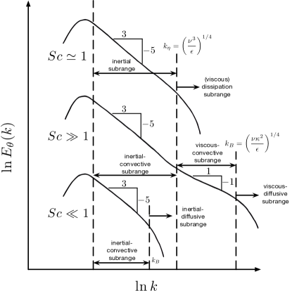
Figure 1: (Color online) Spectra of scalar $E_{\theta}(k)$ for different Schmidt numbers $Sc$. The Kolmogorov scale $k_{\eta}$ and the Batchelor scale $k_{B}$ are illustrated as a vertical dashed line. When $Sc\gg 1$, the so-called Batchelor spectrum $E_{\theta}(k)\propto k^{-1}$ is expected in the range $k_{\eta}\ll k\ll k_{B}$. The figure is reproduced from Tennekes and Lumley (1972).

Concerning a passive scalar $\theta$, e.g., saying dye, temperature, etc., transported by a turbulent velocity field, its small-scale feature is determined by the so-called Schmidt number $\mathrm{Sc}=\nu/\kappa$, where $\kappa$ is the mass diffusive coefficient. It is the ratio between the momentum and mass diffusivity.(Tennekes and Lumley, 1972; Pope, 2000) Three regimes are identified for different $\mathrm{Sc}$, that is, $\mathrm{Sc}\ll 1$, $\mathrm{Sc}=\mathcal{O}(1)$ and $\mathrm{Sc}\gg 1$, respectively. Essentially, $\mathrm{Sc}$ characterizes the scale ratio between the Kolmogorov scale $k_{\eta}$ of the fluid viscosity and the Batchelor scale $k_{B}$ of the passive scalar since mathematically we have $\mathrm{Sc}=(k_{\eta}/k_{B})^{2}$. The power-law behavior of its Fourier power spectrum $E_{\theta}(k)$ is expected for each case. For example, the same scaling behavior of the law $-5/3$ as the velocity behavior in the scaling range $k_{L}\ll k\ll k_{B}$ is expected for $\mathrm{Sc}=\mathcal{O}(1)$ with $k_{B}\simeq k_{\eta}$, which is written as,

$$E_{\theta}(k)\propto\epsilon^{-1/3}\epsilon_{\theta}k^{-5/3},$$ (2)

where $\epsilon_{\theta}$ is the scalar dissipation. This is the so-called Kolmogorov-Obukhov-Corrsin scaling (KOC for short). Obukhov (1949); Corrsin (1951); Warhaft (2000); Sreenivasan (2019) For the regime $\mathrm{Sc}\ll 1$, one still expects the $-5/3$ scaling, but with a shorter inertial-convective subrange than in the KOC case since $k_{B}<k_{\eta}$. A special case is obtained for $\mathrm{Sc}\gg 1$ by Batchelor (1959) that beyond the inertial-convective subrange, there exists an additional viscous-convective subrange $k_{\eta}\ll k$, its Fourier power spectrum is written as,

$$E_{\theta}(k)\propto k^{-1}\exp\left(-(k/k_{B})^{2}\right),$$ (3)

When $k_{\eta}\ll k\ll k_{B}$, an asymptotic behavior suggests a power-law behavior as below,

$$E_{\theta}(k)\propto k^{-1},$$ (4)

These three regimes are summarized in Fig. 1, which is a reproduction of the Figure 8.11 from the classical book by Tennekes and Lumley (1972). Note that the simultaneous observation of the KOC-like $-5/3$ scaling and Batchelor’s $-1$ scaling of passive scalars is difficult because of several reasons for both experiments and simulations. For instance, to pursue both scaling behavior for one decade of scales, one at least needs 3 orders of scale separations in experiment, or 4 orders in numerical simulations since the viscous-diffusive subrange should be well resolved, which are infeasible.(Sreenivasan, 2019) Several attempts have been performed to verify Batchelor’s $-1$ scaling either experimentally or numerically.(Gibson and Schwarz, 1963; Wu et al., 1995; Antonia and Orlandi, 2003; Yeung et al., 2004; Amarouchene and Kellay, 2004; Sreenivasan, 2019; Götzfried et al., 2019; Mohaghar, Dasi, and Webster, 2020; Bedrossian, Blumenthal, and Punshon-Smith, 2022) As mentioned above, it is difficult to realize the $-1$ scaling due to the requirement of a large scale separation. For example, the $-5/3$ Kolmogorov law or KOC scaling is often associated with turbulent flows with a high Reynolds number,(Frisch, 1995) while the Batchelor $-1$ scaling requires that the scalar is locally uniform in space and time when $k\ll k_{\eta}$.(Batchelor, 1959) Thus, controversial results have been reported by several authors.(Sreenivasan, 2019)

One might be curious about the degree to which the flows in those artworks differ from natural flows. For example, using a physics-informed deep learning framework capable of encoding the Navier-Stokes equations into neural networks, Raissi, Yazdani, and Karniadakis (2020) successfully extracted the velocity and pressure fields from Leonardo da Vinci’s painting of turbulent flows. Colagrossi et al. (2021) reproduced the physics behind one of Leonardo da Vinci’s drawings, that is, a water jet impacts a pool, using a smoothed particle hydrodynamic model. They concluded that "He was able to extract essential phenomena of complex air-water flows and accurately describe each flow feature independently from the others, both in his drawings and in their accompanying notes." Krechetnikov (2022a) found that fluid flows in classical paintings are scientific inaccuracies due to a limited understanding of fluid dynamics or deliberately artistic choices.(Krechetnikov, 2022b) Concerning The Starry Night, Aragón et al. (2008) found that the increment of the luminance shows a clear scale invariant, in which their pdfs can be reproduced using the formula from the turbulence community. (Beattie and Kriel, 2019) showed that the corresponding Fourier power spectrum, rather than the Kolmogorov $-5/3$ scaling, is close to $E(k)\propto k^{-2}$, which could be interpreted in the theory of compressible turbulence. However, Finlay (2020) stated that the midrange wavenumber spectrum tends to -1, which is far from the K41. These results seem to contradict each other, partially because only part of the picture is analyzed, in which some of whirls are excluded, see Fig. 2 (b).

In this work, The Starry Night is analyzed after a mask of the church, mountain and village. Both the Fourier power spectrum and the second-order structure function are estimated. Their scaling behaviors are then compared with the prediction of the Batchelor scalar turbulence theory.

II Data and Method

II.1 High Resolution of The Starry Night

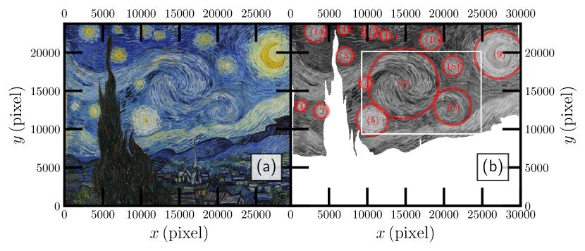
Figure 2: (Color online) (a) a high-resolution van Gogh’s Starry Night obtained from https://artsandculture.google.com with a size $92.1$\mathrm{c}\mathrm{m}$\times 73.7$\mathrm{c}\mathrm{m}$$ and $30,000\times 23,756$ pixels each. Visually, the sky seems to be flowing with swirling eddies. (b) The gray version of the Starry Night, where the region studied by Beattie and Kriel (2019); Finlay (2020) is illustrated by a white square. The non-flow part is masked manually.

The Starry Night is an oil-on-canvas painting by the Dutch postimpressionist painter Vincent van Gogh. Painted in June 1889, it depicts the view from the east-facing window of his asylum room at Saint-Rémy-de-Provence (south of France), just before sunrise, with the addition of an imaginary village. It has been in the permanent collection of the Museum of Modern Art in New York City since 1941, acquired through the Lillie P. Bliss Bequest. Widely regarded as Vincent van Gogh’s magnum opus. The Starry Night is one of the most recognized paintings in western art. Figure 2 shows a high-resolution version of The Starry Night provided by Google Art Project https://artsandculture.google.com with a size $92.1$\mathrm{c}\mathrm{m}$\times 73.7$\mathrm{c}\mathrm{m}$$ and $30,000\times 23,756$ pixels, corresponding to a spatial resolution $\delta x=30\,\mu m$. Visually, fourteen eddies (moon is also included) with different sizes that can be recognized by naked eyes with diameters roughly in the range $4.2\lesssim d\lesssim 27.6\,$\mathrm{c}\mathrm{m}$$ (i.e., $1,400\lesssim d\lesssim 9,200$ pixels), see Tab. 1 in the Appendix. The raw data are converted from red-green-blue to gray to preserve all structures and to exclude the influence of the non-flow-like part, e.g., the church, mountain, and village, they are masked out in the following analysis, see Fig. 2 (b). Moreover, the typical spatial scale of the brushstroke is found to be in the range $0.09\lesssim r\lesssim 1.5\,$\mathrm{c}\mathrm{m}$$ (i.e., $30\lesssim r\lesssim 500$ pixels) for the width and $1.2\lesssim r\lesssim 6\,$\mathrm{c}\mathrm{m}$$ (that is, $400\lesssim r\lesssim 2000\,$ pixels) for the length; see Fig. A.1 in the appendix.

II.2 Methods

II.2.1 Fourier Power Spectrum

As mentioned above that when the flow is turbulent, a power-law behavior of the velocity is expected. In this work, the Fourier power spectrum is estimated via the Wiener-Khinchine theorem since the masked data with missing part, see Fig. 2 (b). The Wiener-Khinchine theorem states that the Fourier power spectrum $E(k)$ of the luminance and the autocorrelation function $\rho(r)$ are a Fourier transform pair, which is written as,

$$E(k)=\int\rho(r)\exp(-j2\pi kr)\mathrm{\,d}r,\,\rho(r)=\int E(k)\exp(j2\pi kr)\mathrm{\,d}k,$$ (5)

where $j=\sqrt{-1}$ is a complex unit, $k=1/r$ is the wavenumber and $r$ is the distance between two points. In practice, the autocorrelation function $\rho(r)$ can be estimated for the case with missing data, in which an additional step is involved to correct the missing data effect, see detail in Ref. Gao et al., 2021. In case of the scale invariant, one expects a power-law behavior of $E(k)$, which is written as,

$$E(k)\propto k^{-\beta},$$ (6)

where $\beta$ is the scaling exponent that can be determined experimentally or theoretical considerations that mentioned above.

II.2.2 Second-order Structure Functions

To characterize the scale invariant in physical space, the second-order structure-function is introduced here as,

$$S_{2}(r)=\langle\Delta_{r}\theta(x)^{2}\rangle\propto r^{\zeta(2)}$$ (7)

where $\theta$ is the luminance; $\Delta_{r}\theta(x)=\theta(x+r)-\theta(x)$ is the scalar difference over distance $r$; $\zeta(2)$ are the second-order scaling exponents if the power law behavior of $E(k)$ holds. A scaling relation $\beta=1+\zeta(2)$ is expected for $1<\beta<3$ (Frisch, 1995; Schmitt and Huang, 2016). However, as discussed by Huang et al. (2010, 2013), due to several reasons, for instance, contamination by the energetic large-scale structure (e.g., ramp-cliff structures in scalar turbulence(Warhaft, 2000; Huang et al., 2011)), ultraviolet or infrared effects, to name a few, it is often violated (Warhaft, 2000; Huang et al., 2010, 2013), see more discussion in Ref. Schmitt and Huang, 2016. Note that for the case of $\mathrm{Sc}\gg 1$, Batchelor theory of scalar turbulence predicts a scaling value of $\beta=1$, and the power law mentioned above in Eq.(7) is then violated due to the ultraviolet effect. Instead of the power law behavior, his theory predicts a log-law, which is written as,

$$S_{2}(r)\propto\alpha\ln(r)$$ (8)

where $r_{B}\ll r\ll r_{\eta}$.

III Results

III.1 Fourier Power Spectrum

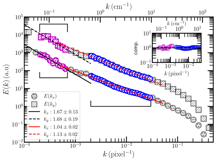
Figure 3: (Color online) Experimental Fourier power spectrum $E(k)$, where the solid and dashed line indicate power-law behavior on the range $6.7\times 10^{-2}\lesssim k\lesssim 2.3\times 10^{-1}\,$\mathrm{c}\mathrm{m}^{-1}$$ (i.e., $2\times 10^{-4}\lesssim k\lesssim 7\times 10^{-4}$ pixel^-1) and $6.7\times 10^{-1}\lesssim k\lesssim 10\,$\mathrm{c}\mathrm{m}^{-1}$$ (i.e., $2\times 10^{-3}\lesssim k\lesssim 3\times 10^{-2}$ pixel^-1). For display clarity, the curve of $E(k_{y})$ has been vertical shifted by multiplying 10. The inset shows the compensated curves using the fitted scaling exponents $\beta$ to emphasize the power-law behavior.

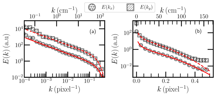
Figure 4: (Color online) Experimental verification of Eq. (3), where solid and dashed lines are least squares fit in the range $6.7\times 10^{-1}\lesssim k\lesssim 1.34\times 10^{2}\,$\mathrm{c}\mathrm{m}^{-1}$$ (i.e., $2\times 10^{-3}\lesssim k\lesssim 4\times 10^{-1}$ pixel^-1): (a) log-log view to highlight the $k^{-1}$, (a) semilog-y view to highlight the tail $\exp\left(-\left(k/k_{B}\right)^{2}\right)$. For display clarity, the curve of $E(k_{y})$ has been vertical shifted by multiplying 10.

The Fourier power spectra $E(k)$ are estimated along horizontal ($x$) and vertical ($y$) directions using the algorithm described in Sec. II.2.1. Figure 3 shows the experimental $E(k)$, where a dual power-law behavior is visible. As mentioned above, the spatial size of the whirls is in the range $4.2\lesssim d\lesssim 27.6\,$\mathrm{c}\mathrm{m}$$ (i.e., $1400\lesssim d\lesssim 9200$ pixels). Therefore, we fit the scaling exponent in the range $6.7\times 10^{-2}\lesssim k\lesssim 2.3\times 10^{-1}\,$\mathrm{c}\mathrm{m}^{-1}$$ (i.e., $2\times 10^{-4}\lesssim k\lesssim 7\times 10^{-4}\,\mathrm{pixel^{-1}}$), corresponding to the range $4.5\lesssim r\lesssim 15\,$\mathrm{c}\mathrm{m}$$ (i.e., $1,500\lesssim r\lesssim 5,000\,$ pixels), for both the horizontal and vertical directions. The experimental scaling exponents are found to be $\beta_{x}=1.67\pm 0.13$ and $\beta_{y}=1.68\pm 0.19$, where the $95\%$ fit confidence is provided by the least squares fit algorithm. These values agree well with the one predicted by the K41/KOC theory, since the scaling range chosen here follows the requirement of the cascade picture that all possible whirls/eddies are included.(Richardson, 1922; Kolmogorov, 1941; Frisch, 1995) .

The experiment scaling exponent of the second power law is estimated in the wavenumber range $6.7\times 10^{-1}\lesssim k\lesssim 10\,$\mathrm{c}\mathrm{m}^{-1}$$ (i.e., $2\times 10^{-3}\lesssim k\lesssim 3\times 10^{-2}\,\mathrm{pixel^{-1}}$), corresponding to the spatial scale in the range $0.1\lesssim r\lesssim 1.5\,$\mathrm{c}\mathrm{m}$$ (i.e., $30\lesssim r\lesssim 500$ pixels). The measured scaling exponents are $\beta_{x}=1.04\pm 0.02$ and $\beta_{y}=1.13\pm 0.02$, (Finlay, 2020) very close to Batchelor "-1" scaling. To highlight the observed scaling behavior, the compensated curve using fitted parameters is shown in Fig. 3 as inset, where clear plateaus are observed. To experimentally verify Eq.3, the least squares fit algorithm to the experiment curve $E(k)$ is performed in the range $6.7\times 10^{-1}\lesssim k\lesssim 1.34\times 10^{2}\,$\mathrm{c}\mathrm{m}^{-1}$$ (i.e., $2\times 10^{-3}\lesssim k\lesssim 4\times 10^{-1}\,\mathrm{pixel^{-1}}$). Visually, Eq. (3) fits well the experimental curve with a Batchelor-like parameter $k_{B}=67\pm 6\,$\mathrm{c}\mathrm{m}^{-1}$$, corresponding to a five pixels, see Fig. 4 (a). To highlight the exponential part $\exp\left(-\left(k/k_{B}\right)^{2}\right)$, $E(k)$ is also reproduced in a semilog-y view, see Fig. 4 (b), confirming the validation of Eq. (3).

III.2 Second-order Structure Functions

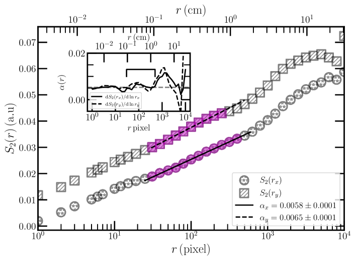
Figure 5: (Color online) Experimental verification of Eq. (8), where solid and dashed lines are least squares fit in the range $0.1\lesssim r\lesssim 1.5\,$\mathrm{c}\mathrm{m}$$ (i.e., $30\lesssim r_{x}\lesssim 500$ pixels) and $0.1\lesssim r\lesssim 0.9\,$\mathrm{c}\mathrm{m}$$ (i.e., $30\lesssim r_{y}\lesssim 300$ pixels). For display clarity, the curve of $S_{2}(r_{y})$ has been vertical shifted by adding $0.01$. The inset shows the local slope $\mathrm{\,d}S_{2}(r)/\mathrm{\,d}\ln(r)$, where the solid horizontal line indicates the range $0.1\lesssim r\lesssim 1.5\,$\mathrm{c}\mathrm{m}$$. The horizontal dash line indicates a mean value $0.0054$ in the range $0.003\lesssim r\lesssim 1.5\,$\mathrm{c}\mathrm{m}$$ (i.e., $1\lesssim r\lesssim 500$ pixels).

As mentioned above, the power law behavior of the second-order structure functions might be violated or strongly biased since we have the ultraviolet effect (e.g., $\beta\simeq 1$ in the range $6.7\times 10^{-2}\lesssim k\lesssim 2.3\times 10^{-1}\,$\mathrm{c}\mathrm{m}^{-1}$$, corresponding to $0.1\lesssim r\lesssim 1.5\,$\mathrm{c}\mathrm{m}$$). Therefore, instead of Eq. (7), the log-law in Eq. (8) is examined. Figure 5 shows the estimated second-order structure functions $S_{2}(r)$. A clear logarithmic law is evident with slopes $0.0058$ and $0.0065$ fitting in the range $0.1\lesssim r\lesssim 1.5\,$\mathrm{c}\mathrm{m}$$ (i.e., $30\lesssim r_{x}\lesssim 500$ pixels) and $0.1\lesssim r\lesssim 0.9\,$\mathrm{c}\mathrm{m}$$ (i.e., $30\lesssim r_{y}\lesssim 300$ pixels), respectively. Note that these ranges of scales agree well with the range of brushstroke widths. The local slope $\mathrm{\,d}S_{2}(r)/\mathrm{\,d}\ln(r)$ is also estimated numerically using a finite center difference; see the inset in Fig. 5. Generally speaking, the local slope has a plateau with a value of $\overline{\alpha}=0.0054\pm 0.009$ in the range $0.003\lesssim r\lesssim 1.5\,$\mathrm{c}\mathrm{m}$$ (i.e., $1\lesssim r\lesssim 500$ pixels). Note that $\alpha(r_{x})$ and $\alpha(r_{y})$ have the same evolution trend with slight difference. It seems that Batchelor’s scalar turbulence theory is a good candidate for interpreting the above results phenomenologically.

IV Discussions

To have Kolmogorov’s $-5/3$ scaling law, a certain number of whirls/eddies should be involved in their statistics to have a wide distribution of scales and so-called interactions among them. Concerning the famous The Starry Night, our results show strong evidence of the $-5/3$ scaling law in the range $6.7\times 10^{-2}\lesssim k\lesssim 2.3\times 10^{-1}\,$\mathrm{c}\mathrm{m}^{-1}$$ when all whirls/eddies are included in our analysis. This is because not only the size distribution of whirls/eddies, but also their relative distance follow the real flow. In other words, Vincent van Gogh had a precise physical mind of turbulent flows. Here, the observed $-5/3$ scaling is due to this mimic of the natural flow.

To satisfy the requirement of the application of Batchelor’s scalar turbulence theory, one should have the Schmidt number $\mathrm{Sc}\gg 1$ and a stationary flow if the flow exists.(Batchelor, 1959) The latter condition is automatically satisfied, since during both preparing the oil and painting the processes are slow enough. We estimate the Reynolds and Schmidt numbers as follows.

IV.1 Estimation of Reynolds number

The characteristic length of the brushstroke is around $4.5\,$\mathrm{c}\mathrm{m}$$. Assuming that the typical time for each brushstroke is $1\,$\mathrm{s}\mathrm{e}\mathrm{c}$$, we see that the typical velocity during the drawing is around $u\simeq 4.5\,$\mathrm{c}\mathrm{m}\mathrm{/}\mathrm{s}$$. So we can estimate the Reynolds number $Re=uL/\nu_{\mathrm{eff}}\simeq 30\propto\mathcal{O}(10)$, where $L$ is the typical spatial scale of $4.5\,$\mathrm{c}\mathrm{m}$$ (i.e., $1500\,$pixels), $\nu_{\mathrm{eff}}$ is the effective kinetic viscosity estimated above. Therefore, in the conventional view, turbulent statistics are not expected, such as the scaling behavior or intermittency effect of high-order statistics. As mentioned above, the observed 5/3 scaling law is due to the fact that not only the size of whirls/eddies but also their relative distances are physical.

IV.2 Estimation of Schmidt number from Fourier spectrum

Note that the observation of the 5/3 scaling law of the Fourier power spectrum is in the range $6.7\times 10^{-2}\lesssim k\lesssim 2.3\times 10^{-1}\,\mathrm{cm^{-1}}$, corresponding to a scale range $4.5\lesssim r\lesssim 15\,\mathrm{cm}$. The Kolmogorov-like scale $\eta_{k}\ll 4.5\,\mathrm{cm}$. The Batchelor-like scaling is observed in the range $6.7\times 10^{-1}\lesssim k\lesssim 10\,\mathrm{cm^{-1}}$, corresponding to a scale range $0.1\lesssim r\lesssim 1.5\,\mathrm{cm}$. The Batchelor-like scale $k_{B}\simeq 67\,\mathrm{cm^{-1}}$ , corresponding to $\eta_{B}\simeq 0.015\,\mathrm{cm}$; see Fig. 4. If we take $1.5\,$\mathrm{c}\mathrm{m}$$ as the Kolmogorov scale, the low bound of the Schmidt number can therefore be estimated as $\mathrm{Sc}=\left(\eta_{k}/\eta_{B}\right)^{2}\simeq\left(1.5/0.015\right)^{2}=\mathcal{O}(10^{4})$.

IV.3 Estimation of Schmidt number from thermal dynamics

According to the Wikipedia,, The Starry Night is an oil-on-canvas painting by Vincent van Gogh in 1889. At that time, the painting oil was made of stone powder and linseed oil. Using classical thermal dynamics knowledge, the effective viscosity and mass diffusive coefficient can be estimated as follows.

Concerning stone powder in linseed oil, we can use a model called the Einstein equation to estimate its effective kinematic viscosity,(Einstein, 1906) which is written as,

$$\mu_{\mathrm{eff}}=\mu_{\mathrm{f}}(1+2.5\phi),$$ (9)

where $\mu_{\mathrm{eff}}$ is the effective dynamic viscosity of the suspension, $\mu_{f}$ is the dynamic viscosity of the fluid, and $\phi$ is the volume fraction of the particles in the suspension. It is an empirical relationship that relates the effective viscosity of a suspension to the properties of the particles and the fluid. When combining the mass ratio of stone powder and linseed oil is $1:1$, the effective viscosity is then,

$$\mu_{\mathrm{eff}}=\mu_{\mathrm{f}}(1+2.5\frac{\rho_{f}}{\rho_{f}+\rho_{s}})$$ (10)

Substituting the given dynamic viscosity of linseed oil $0.06\,$\mathrm{P}\mathrm{a}\cdot\mathrm{s}$$, the density of linseed oil $0.93\,$\mathrm{g}\mathrm{/}\mathrm{c}\mathrm{m}^{3}$$,the density of stone $2.5\,$\mathrm{g}\mathrm{/}\mathrm{c}\mathrm{m}^{3}$$, we get:

$$\mu_{\mathrm{eff}}=1.68\mu_{\mathrm{f}}=1.007\times 10^{-1}\,$\mathrm{P}\mathrm{a}\cdot\mathrm{s}$$$

The effective kinetic viscosity is then estimated as

$$\nu_{\mathrm{eff}}=\frac{\mu_{\mathrm{eff}}}{\rho_{\mathrm{eff}}}\simeq 7.405\times 10^{-5}$\mathrm{m}^{2}\mathrm{/}\mathrm{s}$$$

where the effective fluid density is calculated as $\rho_{\mathrm{eff}}\simeq 1360\,$\mathrm{k}\mathrm{g}\mathrm{/}\mathrm{m}^{3}$$.

Moreover, the diffusion coefficient of a spherical particle in a liquid can be estimated using the Stokes-Einstein equation,(Einstein, 1905; Sadoon, Oliver, and Wang, 2022) which is written as,

$$\kappa=\frac{kT}{6\pi\mu_{\mathrm{f}}r}$$ (11)

where $D$ is the diffusion coefficient, $k$ is the Boltzmann constant, $T$ is the temperature, $\mu_{\mathrm{f}}$ is the dynamic viscosity of the liquid, and $r$ is the radius of the spherical particle. We estimate here an order of the Schmidt number; therefore, we do not consider a non-spherical particle or a mixture of particle sizes, where more complex models may be required. Assuming an average particle radius of $r=10\,$\mu\mathrm{m}$$ and a dynamic viscosity of the linseed oil at room temperature ($T=293.15\,$\mathrm{K}$$) of $3.36\times 10^{-5}\,$\mathrm{P}\mathrm{a}\cdot\mathrm{s}$$, the mass diffusivity of the stone powder in the linseed oil can be estimated to be around $\kappa\simeq 1.6\times 10^{-14}$\mathrm{m}^{2}\mathrm{/}\mathrm{s}$$. Finally, we have an estimation of Schmidt number as,

$$\mathrm{Sc}=\frac{\nu_{\mathrm{eff}}}{\kappa}\simeq 4.63\times 10^{9}=\mathcal{O}(10^{9})$$

This value is above the value of the low bound estimated from Fourier power spectrum. It is important to note that the above estimation assumes that the particles are small enough so that they do not interact with each other, which may not be the case for more concentrated suspensions or for particles with complex shapes.

IV.4 Batchelor scalar turbulence

As mentioned above, the prediction of "-1" scaling by the Batchelor scalar turbulence theory is difficult to realize not only in the meaning of the experiment but also in numerical simulation. Several attempts have been made to verify this theory. For example, Amarouchene and Kellay (2004) observed the Batchelor scaling for the thickness fluctuation of fast-flowing soap films. However, to fit the experiment spectrum curve, instead of Batchelor’s original proposal $k^{-1}\exp\left(-\left(k/k_{B}\right)^{2}\right)$, an exponential tail is considered, that is, $k^{-1}\exp\left(-k/k_{B}\right)$, the form proposed by Kraichnan (1968) when the fluctuation of the strain is taken into account. Here we can fit the experiment curve using his original proposal, since the requirement of an application of his scalar turbulence theory is satisfied.

V Conclusion

In summary, we show in this work that if we strictly follow the requirement of the turbulence theory, the turbulence-like statistics can be recovered for The Starry Night, e.g., the Kolmogorov $-5/3$ scaling, Batchelor $-1$ scaling for the Fourier power spectrum, etc. Or, in other words, Vicent van Gogh had a very careful observation of the turbulent flow that not only the size of whirls/eddies, but also their relative distance in The Starry Night do correct mimic the law of physics. Furthermore, the full Batchelor spectrum (i.e., Eq. (3)) is evident when the spatial scale is below the visual whirls/eddies. This is because during the preparation of the painting oil and the drawing process, the characteristic Reynolds number is low and the diffusivity is dominant. Moreover, the second-order structure function also follows the theoretical prediction, showing a log-dependence. Therefore, the hidden turbulence in The Starry Night is recovered and explained using turbulent theories.

AUTHOR DECLARATIONS

Conflict of Interest

The authors have no conflicts to disclose.

Author Contributions

Y.X. Huang: Conceptualization (lead); Formal analysis (lead); Investigation (lead); Writing - review & editing (lead). Y.X. Ma: Formal analysis (supporting); Methodology (supporting); Writing - review & editing (supporting). S.D. Huang: Formal analysis (supporting); Investigation (supporting); Writing - review & editing (supporting). W.T. Cheng: Formal analysis (supporting); Investigation (supporting); Writing - review & editing (supporting). F.G. Schmitt: Formal analysis (supporting); Investigation (supporting); Writing - review & editing (supporting).

VI DATA AVAILABILITY

The data that support the findings of this study are available at https://artsandculture.google.com. A copy of the source code for the present analysis is available at https://github.com/lanlankai.

Appendix A Typical Spatial Scales

As aforementioned, the detection of the scaling range should follow the requirement of the turbulent theory that enough structures should be involved. Here, we count the typical spatial scale manually for both visualized whirls and brush strokes.

A.0.1 Spatial scales of whirls

The spatial sizes of fourteen whirls/eddies are estimated by naked eyes. Their diameters, location, and area are list in Tab. 1. Following Richardson’s picture of the cascade, the Kolmogorov 1941 scaling is then expected in the range $1,400\lesssim r\lesssim 9,200$ pixels (i.e., $4.3\lesssim r\lesssim 28.2\,$\mathrm{c}\mathrm{m}$$), corresponding to a wavenumber in range $1\times 10^{-4}\lesssim k\lesssim 7\times 10^{-4}\,\mathrm{pixel^{-1}}$ (i.e., $3\times 10^{-2}\lesssim r\lesssim 2\times 10^{-1}\,$\mathrm{c}\mathrm{m}$^{-1}$).

Table 1: Eddy geometric property checked manually by naked eyes. The diameters of the whirls/eddies are roughly on the range $1,400\sim 9,200$ pix (i.e., $4.3\sim 28.2,$\mathrm{c}\mathrm{m}$$), corresponding to a scale ratio around $\simeq 6.8$. The Kolmogorov-like five-third scaling law is expected in this range.

No.	$D$ (pix/$\mathrm{c}\mathrm{m}$)	location x (pixel)	location y (pixel)	area (pixel2/$$\mathrm{c}\mathrm{m}$^{2}$)
1	1,500/4.6	1,356	10,740	1,730,000/16.3
2	1,900/5.8	3,996	11,386	2,790,000/26.3
3	2,200/6.8	7,106	4,173	3,850,000/36.3
4	1,700/5.3	9,790	7,750	2,130,000/20.1
5	4,100/12.6	10,628	12,560	1,320,000/12.4
6	4,800/14.7	21,130	10,837	18,340,000/172.9
7	9,200/28.2	14,698	7,817	67,250,000/633.8
8	2,600/8.0	21,163	5,532	5,480,000/51.6
9	6,300/19.3	27,140	4,017	31,470,000/296.6
10	2,800/8.6	18,275	2,053	6,230,000/58.7
11	1,400/4.3	12,372	1,591	1,580,000/14.9
12	2,000/6.1	10,332	970	3,160,000/29.8
13	1,500/4.6	6,905	724	1,770,000/16.7
14	2,800/8.6	3,222	1,036	5,990,000/56.5

A.0.2 Spatial scales of brushstrokes

The spatial scale of brushstrokes are estimated manually with a minimum and maximum width around $30\,$ and $500\,$pixels (i.e., $9.2\times 10^{-2}\lesssim r\lesssim 1.5\,$\mathrm{c}\mathrm{m}$$). Figure A.1 shows an example for three typical whirls/eddies. The Batchelor’s "-1" law is then expected in this range.

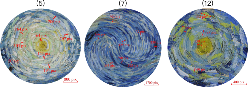
Figure A.1: (Color online) Manually check the width of brushstrokes for the Nos. (5), (7) and (12) eddies of the high resolution case. The width is found roughly on the range $50\sim 400$ pix (i.e., $1.5\times 10^{-1}\lesssim r\lesssim 1.2\,$\mathrm{c}\mathrm{m}$$). The variation of the luminance on this range is partially due to the preparation of painting oil, diffusion of the solid particles.

References

- Frisch (1995) U. Frisch, Turbulence: the legacy of AN Kolmogorov (Cambridge University Press, 1995).
- Wensink et al. (2012) H. H. Wensink, J. Dunkel, S. Heidenreich, K. Drescher, R. E. Goldstein, H. Löwen, and J. M. Yeomans, “Meso-scale turbulence in living fluids,” Proc. Natl. Acad. Sci. 109, 14308–14313 (2012).
- Qiu et al. (2016) X. Qiu, L. Ding, Y. Huang, M. Chen, Z. Lu, Y. Liu, and Q. Zhou, “Intermittency measurement in two-dimensional bacterial turbulence,” Phys. Rev. E 93, 062226 (2016).
- Mantegna and Stanley (1996) R. Mantegna and H. Stanley, “Turbulence and financial markets,” Nature 383, 587–588 (1996).
- Schmitt, Schertzer, and Lovejoy (2000) F. Schmitt, D. Schertzer, and S. Lovejoy, “Multifractal fluctuations in finance,” Int. J. Theor. Appl. Fin. 3, 361–364 (2000).
- Li and Huang (2014) M. Li and Y. Huang, “Hilbert–Huang Transform based multifractal analysis of China stock market,” Physica A 406, 222–229 (2014).
- Zhou (2021) Y. Zhou, “Turbulence theories and statistical closure approaches,” Phys. Rep. 935, 1–117 (2021).
- Warhaft (2022) Z. Warhaft, “The art of turbulence,” American Scientist 110, 360–367 (2022).
- Chen, Yang, and Jiang (2019) G. Chen, S. Yang, and N. Jiang, “Leonardo da vinci and fluid mechanics,” Mech. Eng. (in Chinese) 41, 634 (2019).
- Raissi, Yazdani, and Karniadakis (2020) M. Raissi, A. Yazdani, and G. E. Karniadakis, “Hidden fluid mechanics: Learning velocity and pressure fields from flow visualizations,” Science 367, 1026–1030 (2020).
- Marusic and Broomhall (2021) I. Marusic and S. Broomhall, “Leonardo da Vinci and fluid mechanics,” Ann. Rev. Fluid Mech. 53, 1–25 (2021).
- Colagrossi et al. (2021) A. Colagrossi, S. Marrone, P. Colagrossi, and D. Le Touzé, “Da vinci’s observation of turbulence: A french-italian study aiming at numerically reproducing the physics behind one of his drawings, 500 years later,” Phys. Fluids 33 (2021), 10.1063/5.0070984.
- Ornes (2014) S. Ornes, “Science and culture: Dissecting the great wave,” Proc. Natl. Acad. Sci. 111, 13245–13245 (2014).
- Aragón et al. (2008) J. L. Aragón, G. G. Naumis, M. Bai, M. Torres, and P. K. Maini, “Turbulent luminance in impassioned van Gogh paintings,” J. Math. Imaging Vision 30, 275–283 (2008).
- Olson (2014) D. W. Olson, Celestial Sleuth: Using Astronomy to Solve Mysteries in Art, History and Literature (Springer, 2014).
- Beattie and Kriel (2019) J. Beattie and N. Kriel, “Is the Starry Night turbulent?” arXiv preprint (2019), 10.48550/arXiv.1902.03381.
- Finlay (2020) W. H. Finlay, “The midrange wavenumber spectrum of van Gogh’s Starry Night does not obey a turbulent inertial range scaling law,” J. Turbul. 21, 34–38 (2020).
- Richardson (1922) L. Richardson, Weather prediction by numerical process (Cambridge University Press, Cambridge, England,, 1922).
- Alexakis and Biferale (2018) A. Alexakis and L. Biferale, “Cascades and transitions in turbulent flows,” Phys. Rep. 767, 1–101 (2018).
- Kolmogorov (1941) A. N. Kolmogorov, “Local structure of turbulence in an incompressible fluid at very high Reynolds numbers,” Dokl. Akad. Nauk SSSR 30, 301 (1941).
- Pope (2000) S. Pope, Turbulent Flows (Cambridge University Press, 2000).
- Tsinober (2009) A. Tsinober, An informal conceptual introduction to turbulence (Springer Verlag, 2009).
- Tennekes and Lumley (1972) H. Tennekes and J. L. Lumley, A First Course in Turbulence (MIT Press, 1972).
- Groisman and Steinberg (2000) A. Groisman and V. Steinberg, “Elastic turbulence in a polymer solution flow,” Nature 405, 53–55 (2000).
- Wang and Huang (2017) L. Wang and Y. Huang, “Intrinsic flow structure and multifractality in two-dimensional bacterial turbulence,” Phys. Rev. E 95, 052215 (2017).
- Jian et al. (2019) X. Jian, W. Zhang, Q. Deng, and Y. Huang, “Turbulent lithosphere deformation in the tibetan plateau,” Phys. Rev. E 99, 062122 (2019).
- Obukhov (1949) A. M. Obukhov, “Structure of the temperature field in a turbulent flow,” Izv. Acad. Nauk SSSR Ser. Geog. Geofiz 13, 58–69 (1949).
- Corrsin (1951) S. Corrsin, “On the spectrum of isotropic temperature fluctuations in an isotropic turbulence,” J. Appl. Phys. 22, 469 (1951).
- Warhaft (2000) Z. Warhaft, “Passive scalars in turbulent flows,” Annu. Rev. Fluid Mech. 32, 203–240 (2000).
- Sreenivasan (2019) K. R. Sreenivasan, “Turbulent mixing: A perspective,” Proc. Natl. Acad. Sci. 116, 18175–18183 (2019).
- Batchelor (1959) G. K. Batchelor, “Small-scale variation of convected quantities like temperature in turbulent fluid part 1. general discussion and the case of small conductivity,” J. Fluid Mech. 5, 113–133 (1959).
- Gibson and Schwarz (1963) C. Gibson and W. Schwarz, “The universal equilibrium spectra of turbulent velocity and scalar fields,” J. Fluid Mech. 16, 365–384 (1963).
- Wu et al. (1995) X. Wu, B. Martin, H. Kellay, and W. Goldburg, “Hydrodynamic convection in a two-dimensional couette cell,” Phys. Rev. Lett. 75, 236 (1995).
- Antonia and Orlandi (2003) R. Antonia and P. Orlandi, “Effect of schmidt number on small-scale passive scalar turbulence,” Appl. Mech. Rev. 56, 615–632 (2003).
- Yeung et al. (2004) P. Yeung, S. Xu, D. Donzis, and K. Sreenivasan, “Simulations of three-dimensional turbulent mixing for schmidt numbers of the order 1000,” Flow Turbul. Combust. 72, 333–347 (2004).
- Amarouchene and Kellay (2004) Y. Amarouchene and H. Kellay, “Batchelor scaling in fast-flowing soap films,” Phys. Rev. Lett. 93, 214504 (2004).
- Götzfried et al. (2019) P. Götzfried, M. S. Emran, E. Villermaux, and J. Schumacher, “Comparison of lagrangian and eulerian frames of passive scalar turbulent mixing,” Phys. Rev. Fluids 4, 044607 (2019).
- Mohaghar, Dasi, and Webster (2020) M. Mohaghar, L. P. Dasi, and D. R. Webster, “Scalar power spectra and turbulent scalar length scales of high-schmidt-number passive scalar fields in turbulent boundary layers,” Phys. Rev. Fluids 5, 084606 (2020).
- Bedrossian, Blumenthal, and Punshon-Smith (2022) J. Bedrossian, A. Blumenthal, and S. Punshon-Smith, “The batchelor spectrum of passive scalar turbulence in stochastic fluid mechanics at fixed reynolds number,” Comm. Pure Appl. Math. 75, 1237–1291 (2022).
- Krechetnikov (2022a) R. Krechetnikov, “Depictions of fluid phenomena in art,” Nat. Phys. 18, 1256–1259 (2022a).
- Krechetnikov (2022b) R. Krechetnikov, “Fluids in art:" the water’s language was a wondrous one, some narrative on a recurrent subject…",” arXiv preprint (2022b), 10.48550/arXiv.2208.05511.
- Gao et al. (2021) Y. Gao, F. G. Schmitt, J. Y. Hu, and Y. X. Huang, “Scaling analysis of the China France Oceanography SATellite along-track wind and wave data,” J. Geophys. Res. Oceans 126, e2020JC017119 (2021).
- Schmitt and Huang (2016) F. G. Schmitt and Y. Huang, Stochastic Analysis of Scaling Time Series: From Turbulence Theory to Applications (Cambridge Univ Press, 2016).
- Huang et al. (2010) Y. Huang, F. Schmitt, Z. Lu, P. Fougairolles, Y. Gagne, and Y. Liu, “Second-order structure function in fully developed turbulence,” Phys. Rev. E 82, 026319 (2010).
- Huang et al. (2013) Y. Huang, L. Biferale, E. Calzavarini, C. Sun, and F. Toschi, “Lagrangian single particle turbulent statistics through the Hilbert-Huang Transforms,” Phys. Rev. E 87, 041003(R) (2013).
- Huang et al. (2011) Y. Huang, F. Schmitt, J.-P. Hermand, Y. Gagne, Z. Lu, and Y. Liu, “Arbitrary-order Hilbert spectral analysis for time series possessing scaling statistics: comparison study with detrended fluctuation analysis and wavelet leaders,” Phys. Rev. E 84, 016208 (2011).
- Note (1) https://en.wikipedia.org.
- Einstein (1906) A. Einstein, “Eine neue bestimmung der moleküldimensionen,” Annalen der Physik 4 (1906), 10.1002/andp.19063240204.
- Note (2) We estimate here the order of Schmidt number, therefore the value of this ratio does not change our conclusion.
- Einstein (1905) A. Einstein, “Üon the movement of particles suspended in resting liquids required by the molecular kinetic theory of heat ä [adp 17, 549 (1905)],” Annals of Physics 322, 549 (1905).
- Sadoon, Oliver, and Wang (2022) A. A. Sadoon, W. F. Oliver, and Y. Wang, “Revisiting the temperature dependence of protein diffusion inside bacteria: Validity of the stokes-einstein equation,” Phys. Rev. Lett. 129, 018101 (2022).
- Kraichnan (1968) R. H. Kraichnan, “Small-scale structure of a scalar field convected by turbulence,” Phys. Fluids 11, 945–953 (1968).