Non-perturbative mass renormalization effects in
non-relativistic quantum electrodynamics

Abstract

This work lays the foundation to accurately describe ground-state properties in multimode photonic environments and highlights the importance of the mass renormalization procedure for ab initio quantum electrodynamics simulations. We first demonstrate this for free particles, where the energy dispersion is employed to determine the mass of the particles. We then show how the multimode photon field influences various ground and excited-state properties of atomic and molecular systems. For instance, we observe the enhancement of localization for the atomic system, and the modification of the potential energy surfaces of the molecular dimer due to photon-mediated long-range interactions. These phenomena get enhanced under strong light-matter coupling in a cavity environment and become relevant for the emerging field of polaritonic chemistry. We conclude by demonstrating how non-trivial ground-state effects due to the multimode field can be accurately captured by approximations that are simple and numerically feasible even for realistic systems.

I Introduction

In recent years, a multitude of seminal experimental and theoretical breakthroughs involving atoms, molecules, and solids embedded in photonic structures have ushered in the rapidly developing fields of polaritonic chemistry Ruggenthaler et al. (2018); Flick et al. (2018); Ruggenthaler et al. (2023) and cavity quantum materials Schlawin et al. (2022); Ebbesen (2016); Garcia-Vidal et al. (2021). The common and important aspect of these fields is the capability of modifying or controlling the properties of matter in an unprecedented way by coupling it strongly to the vacuum modes of a photonic structure. Some examples of the experimental and theoretical works include the possibility of building polariton lasers Kéna-Cohen and Forrest (2010), control photochemical reactions Hutchison et al. (2012); Galego et al. (2016) and energy transfer Coles et al. (2014); Schäfer et al. (2019); Zhong et al. (2016), enhancement of harmonic generation from polaritonic states Chervy et al. (2016); Barachati et al. (2018); Welakuh and Narang (2023, 2022a), modification of ground-state chemical reactions via vibrational strong coupling Thompson et al. (2006); Schäfer et al. (2022); Thomas et al. (2019), or cavity-control of condensed matter properties Peter et al. (2005); Latini et al. (2021); Liu et al. (2015); Appugliese et al. (2022); Paravicini-Bagliani et al. (2019); Rokaj et al. (2022a, 2023a). Also, the coupled light-matter system can be tuned to exhibit significantly different properties even at room temperature Chikkaraddy et al. (2016); Ojambati et al. (2019). The variety of these different effects (which is by no means a comprehensive list) shows the complexity that results from a strongly coupled light-matter system. It is clear that the theoretical description of these effects is far from trivial as it requires knowledge and methods ranging from materials science, quantum chemistry, quantum optics and many-body physics.

The theoretical tools employed to explain the experimental results are commonly quantum optical models (e.g., Tavis-Cummings or Dicke-model) Dicke (1954); Tavis and Cummings (1968), and only recently first-principles approaches for coupled light-matter systems have been developed Ruggenthaler et al. (2014); Flick et al. (2015); Haugland et al. (2020); Riso et al. (2022). These approaches, often formulated for a continuum of photonic modes, commonly make the few- or even single-effective-mode approximation in practice Galego et al. (2017); Gonzalez-Ballestero et al. (2016). While this approximation is often well-justified, there are many effects that need a multi-mode description Ruggenthaler et al. (2023). Examples include radiative dissipation and finite-lifetime effects, such as the Purcell effect Purcell (1995), dispersive forces (Casimir and van der Walls forces) Casimir and Polder (1948) or renormalization effects such as the Lamb-shift Bethe and Salpeter (1957). In the case of quantum optical models many multi-mode effects have been studied in detail Weisskopf and Wigner (1930); Bužek et al. (1999); Flick et al. (2017), yet due to the reduced nature of the matter degrees of freedom (an apriori reduction to a few effective levels), renormalization and its connection with bare matter quantities has been studied less. For the case of first-principles methods, however, it has been pointed out that the necessary renormalization of the masses of the charged particles can have a strong effect Spohn (2004); Ruggenthaler et al. (2023). Given the fact that the electromagnetic environment in a cavity is drastically different than free space, because the photon density of states, electromagnetic spectrum and light-matter coupling are modified, it becomes necessary to investigate how multimode renormalization effects in the cavity emerge under strong coupling. Having in mind the recent successes in experimentally modifying chemical reactions and material properties, these effects could be part of the solution to the conundrum of how photon-field fluctuations can influence atoms, molecules and solid-state systems. In order to quantify the effects on equilibrium states, a non-perturbative investigation that solves the coupled light-matter problem exactly is needed.

Such a study is, however, far from trivial and we need to make some initial assumptions to make it tractable. Firstly, since we are mainly interested in the effect of optical wavelengths on bound-state systems, we make the long-wavelength approximation (also called dipole-approximation or optical limit Cohen‐Tannoudji et al. (1989); Spohn (2004)). This is the common standard in most cases of polaritonic chemistry and material sciences Ruggenthaler et al. (2018); Schlawin et al. (2022); Ebbesen (2016). In this case the connection between the necessary regularization of the light-matter interaction, which in its simplest form is merely a cutoff at some highest energy, and the bare mass of low-energy quantum-electrodynamics (QED) Spohn (2004) is known analytically from perturbation theory Hainzl and Seiringer (2002). This (together with choosing different gauges) allows us to verify the accuracy of our numerical simulations when going from free particles to bound-state systems. Secondly, in order to represent the continuum of modes numerically, we require a dense sampling of the relevant energy range. For a non-perturbative simulation this becomes exceptionally demanding for three-dimensions. We will therefore restrict to a one-dimensional continuum of modes and respective atomic and molecular models Flick et al. (2017); Landau and Lifshitz (1977); Albareda et al. (2021). We will comment on the range of validity of these two assumptions and on the implications of our results for general situations later.

Having set the stage, we in the following first discuss free-space mass-renormalization in non-perturabtive QED. This introduces the concept of a bare mass in a way that is most closely connected to the common renormalization procedure of perturbative QED Hainzl and Seiringer (2002); Mandl and Shaw (2010). We demonstrate how the mass renormalization procedure introduces the experimentally observable renormalized mass and correctly obtains the energy dispersion from a quantum mechanics calculation. Going beyond this standard setting we then show how the continuum of modes influences the ground state of atomic and molecular systems. Interestingly we find that the renormalized (effective) mass approximation, as employed in matter-only quantum mechanics, shows relatively strong deviations from the full multi-mode simulations. The discrepancies become more pronounced when going to the molecular case. These results highlight an important feature of multimode light-matter interaction for bound matter systems were the lower-lying modes of the sampled electromagnetic continuum couples strongly and influences equilibrium properties when compared to the higher-lying modes. We then show how modifying the electromagnetic vacuum by, e.g., an optical cavity, can affect the ground state properties of atomic and molecular systems. For the atomic model we find that the ground state density of the electron gets an enhancement of localization due to the interaction with the multimode cavity field. For the molecular $H_{2}$ model we observe the modification of the ground state PES due to cavity-mediated long-range interactions. These results are important for the emerging field of polaritonic chemistry and could potentially guide future developments in the cavity control of chemistry. Finally we demonstrate how many of the counter-intuitive and non-trivial ground-state effects can be captured by a specifically-chosen effective few-mode or dipole-self-energy approximation. These approximations allow to capture multi-mode induced ground-state modifications in realistic material systems.

II Theoretical framework

We start by presenting the non-relativistic limit of QED to describe the interaction of the electrons, photons and nuclei. This description of the coupled light-matter system considers transverse fields with wavelengths that are substantially larger than the matter system so that the long-wavelength limit Cohen‐Tannoudji et al. (1989) is applicable. In this non-relativistic setting, the dynamics of the coupled system is described by the velocity (momentum) form of the Pauli-Fierz Hamiltonian Rokaj et al. (2018); Spohn (2004):

$$\hat{H}_{\text{V}} =\sum\limits_{l=1}^{N_{e}}\frac{1}{2m}\left(-i\hbar\boldsymbol{\nabla}_{\textbf{r}_{l}}-\frac{|e|}{c}\hat{\textbf{A}}\right)^{2}+\frac{1}{2}\sum\limits_{l\neq j}^{N_{e}}w(|\hat{\textbf{r}}_{l}-\hat{\textbf{r}}_{j}|)$$

$$\quad+\sum\limits_{l=1}^{N_{n}}\frac{1}{2M_{l}}\left(-i\hbar\boldsymbol{\nabla}_{\textbf{R}_{l}}+\frac{Z_{l}|e|}{c}\hat{\textbf{A}}\right)^{2}$$

$$\quad+\frac{1}{2}\sum\limits_{l\neq j}^{N_{n}}Z_{l}Z_{j}w(|\hat{\textbf{R}}_{l}-\hat{\textbf{R}}_{j}|)+\sum_{\alpha=1}^{N_{p}}\hbar\omega_{\alpha}\left(\hat{a}^{\dagger}_{\alpha}\hat{a}_{\alpha}+\tfrac{1}{2}\right)$$

$$\quad-\sum\limits_{l=1}^{N_{e}}\sum\limits_{j=1}^{N_{n}}Z_{j}w(|\hat{\textbf{r}}_{l}-\hat{\textbf{R}}_{j}|),$$ (1)

where the positive parameters $m$ and $M_{l}$ are the bare masses of the $N_{e}$ electrons and $N_{n}$ nuclei, respectively. The electrons and nuclei are respectively described by the coordinates, $\hat{\textbf{r}}_{l}$ and $\hat{\textbf{R}}_{l}$, and $w$ is the longitudinal interaction between the charged particles. In free space and in three dimensions it is the usual Coulomb interaction $w(|\hat{\textbf{r}}-\hat{\textbf{r}}^{\prime}|)=e^{2}/4\pi\varepsilon_{0}|\hat{\textbf{r}}-\hat{\textbf{r}}^{\prime}|$. The energy of the quantized electromagnetic field is given in terms of the photon creation $\hat{a}^{\dagger}_{\alpha}$ and annihilation $\hat{a}_{\alpha}$ operators with associated mode frequency $\omega_{\alpha}$ for each mode $\alpha$ of an arbitrarily large but finite number of photon modes $N_{p}$. The vector potential is $\hat{\textbf{A}}=\sum_{\alpha=1}^{N_{p}}c\,\boldsymbol{\lambda}_{\alpha}\sqrt{\hbar/2\omega_{\alpha}}\left(\hat{a}_{\alpha}+\hat{a}_{\alpha}^{\dagger}\right)$ where $\boldsymbol{\lambda}_{\alpha}=\sqrt{1/\epsilon_{0}V_{\alpha}}\textbf{e}_{\alpha}$ is the coupling parameter and $V_{\alpha}$ is the mode volume of the mode $\alpha$. The collective index $\alpha\equiv(\textbf{k}s)$ is used denote the photon wavevector and the two transversal polarization directions $s=1,2$. We note that when sampling the photon modes, we cannot go to arbitrary high photon momenta $|\textbf{k}|\rightarrow\infty$, otherwise the Pauli-Fierz Hamiltonian in the long-wavelength approximation will be ill-defined Spohn (2004). This mathematical fact is quite easy to understand on physical grounds, since arbitrarily high momenta directly contradict the basic assumption of the long-wavelength approximation. Any microscopic length scale would be resolved with arbitrarily high frequencies. To circumvent this, the contributions of the photon continuum needs to be regularized by introducing an ultraviolet cutoff Spohn (2004); Hainzl and Seiringer (2002).

It is important to note that the coupled light-matter system can be studied using the unitary equivalent form of Eq. (1) Rokaj et al. (2018), the so-called length form of the Pauli-Fierz Hamiltonian given as:

$$\hat{H}_{\text{L}} =-\frac{\hbar^{2}}{2m}\sum\limits_{l=1}^{N_{e}}\boldsymbol{\nabla}_{\textbf{r}_{l}}^{2}-\sum\limits_{l=1}^{N_{n}}\frac{\hbar^{2}}{2M_{l}}\boldsymbol{\nabla}_{\textbf{R}_{l}}^{2}+\frac{1}{2}\sum\limits_{l\neq j}^{N_{e}}w(|\hat{\textbf{r}}_{l}-\hat{\textbf{r}}_{j}|)$$

$$\quad+\frac{1}{2}\sum\limits_{l\neq j}^{N_{n}}Z_{l}Z_{j}w(|\hat{\textbf{R}}_{l}-\hat{\textbf{R}}_{j}|)\!-\!\sum\limits_{l=1}^{N_{e}}\sum\limits_{j=1}^{N_{n}}Z_{j}w(|\hat{\textbf{r}}_{l}-\hat{\textbf{R}}_{j}|)$$

$$\quad+\frac{1}{2}\sum_{\alpha=1}^{M}\left[\hat{p}^{2}_{\alpha}+\omega^{2}_{\alpha}\left(\hat{q}_{\alpha}\!-\!\frac{\boldsymbol{\lambda}_{\alpha}}{\omega_{\alpha}}\cdot\hat{\boldsymbol{\mu}}\right)^{2}\right],$$ (2)

where the total dipole is $\hat{\boldsymbol{\mu}}=-\sum_{l=1}^{N_{e}}|e|\,\hat{\textbf{r}}_{l}+\sum_{l=1}^{N_{n}}Z_{l}e\hat{\textbf{R}}_{l}$, $\hat{q}_{\alpha}$ is the displacement coordinate and $\hat{p}_{\alpha}=-i\hbar\tfrac{\partial}{\partial\hat{q}_{\alpha}}$ its conjugate momentum. We can define new creation and annihilation operators also for the length gauge, but we note that they are not the original photonic operators as defined above in the velocity gauge but are mixed light-matter objects Rokaj et al. (2018); Schäfer et al. (2020). The explicit interaction of the matter degrees of freedom with the photons as in Eqs. (1) and (2), requires that we work with the bare masses. The reason being that the masses in Eqs. (1) and (2) are not the observable (or physical) mass that is used in standard quantum mechanics. By quantum mechanics we are referring to the dynamics of only interacting electrons and nuclei described by the Hamiltonian

$$\hat{H}_{\text{QM}} =-\frac{\hbar^{2}}{2m_{e}}\sum\limits_{l=1}^{N_{e}}\boldsymbol{\nabla}_{\textbf{r}_{l}}^{2}-\sum\limits_{l=1}^{N_{n}}\frac{\hbar^{2}}{2M_{n,l}}\boldsymbol{\nabla}_{\textbf{R}_{l}}^{2}$$

$$\quad+\frac{1}{2}\sum\limits_{l\neq j}^{N_{e}}w(|\hat{\textbf{r}}_{l}-\hat{\textbf{r}}_{j}|)+\frac{1}{2}\sum\limits_{l\neq j}^{N_{n}}Z_{l}Z_{j}w(|\hat{\textbf{R}}_{l}-\hat{\textbf{R}}_{j}|)$$

$$\quad-\sum\limits_{l=1}^{N_{e}}\sum\limits_{j=1}^{N_{n}}Z_{j}w(|\hat{\textbf{r}}_{l}-\hat{\textbf{R}}_{j}|)\,,$$ (3)

where $m_{e}$ and $M_{n,l}$ are the renormalized or observable masses of the electrons and nuclei, respectively. In the quantum mechanics setting, the observable mass of the particles is derived from non-relativistic QED by tracing out the photon degrees and including their contributions $m_{pt}$ and $M_{l,pt}$ approximately in $m_{e}$ and $M_{n,l}$. This leads to a relation between the bare and the observable masses of the form Spohn (2004); Hainzl and Seiringer (2002); Craig and Thirunamachandran (1998)

$$m_{e} =m+m_{pt}\,,$$ (4)

$$M_{n,l} =M_{l}+M_{pt,l}\,.$$ (5)

The photon-induced masses $m_{pt}$ and $M_{pt,l}$ are interpreted respectively as the masses acquired by the electrons and nuclei due to the interaction with the photon field Craig and Thirunamachandran (1998), and the bare masses $m$ and $M_{l}$ are chosen to represent the contribution from the matter degrees that depends on how the electromagnetic modes decay for increasing photon frequencies Hainzl and Seiringer (2002). In the following we want to investigate the influence of the bare masses on important properties of atomic and molecular systems, specifically if we change the environment due to an optical cavity. But before we do so, let us consider how commonly the bare and the observable masses are related Craig and Thirunamachandran (1998); Spohn (2004); Hainzl and Seiringer (2002).

III Free particles coupled to the electromagnetic continuum

To elucidate how non-relativistic QED and quantum mechanics are commonly related we consider the dispersion relation of free charged particles. We will use the case of free electrons in the following, but note that we can merely replace the charges and bare masses in the different formulas and also find the corresponding forms for the nuclei. We describe the free electrons coupled to the modes from Eq. (1) by dropping all the terms of the nuclei and its coupling to the photon field as well as setting the longitudinal interactions $w$ to zero. Employing periodic boundary conditions for electrons, the electronic eigenstates are plane waves and the exact, nonperturbative spectrum of the non-interacting electrons was found analytically in Ref. Rokaj et al. (2022b) and is given by

$$E_{\textbf{k}}(N_{p}) =\frac{\hbar^{2}}{2m}\left(\sum_{j=1}^{N_{e}}\textbf{k}_{j}^{2}-\frac{1}{N_{e}}\sum_{\alpha=1}^{N_{p}}\frac{\omega_{d}^{2}}{\Omega_{\alpha}^{2}}(\tilde{\textbf{e}}_{\alpha}\cdot\textbf{K})^{2}\right)$$

$$\quad+\sum_{\alpha=1}^{N_{p}}\hbar\Omega_{\alpha}\left(n_{\alpha}+\frac{1}{2}\right)\,,$$ (6)

where $\Omega_{\alpha}$ and $\tilde{\textbf{e}}_{\alpha}$ are the new normal modes and the new polarization vectors, the diamagnetic frequency of the system is defined as $\omega_{d}=\sqrt{{N_{e}e^{2}}/{\epsilon_{0}mV_{\alpha}}}$ and $\textbf{K}=\sum_{j=1}^{N_{e}}\textbf{k}_{j}$ is the sum of all electronic momenta. To obtain the quantum mechanics eigenspectrum for the non-interacting free electron gas from Eq. (6), we can subsume the contributions of the photonic degrees and its interaction with the electronic system into the observable mass and express the eigenspectrum defined in Eq. (6) as

$$E_{\textbf{k}}=\frac{\hbar^{2}}{2m_{e}}\sum_{j=1}^{N_{e}}\textbf{k}_{j}^{2}\,.$$ (7)

In non-relativistic QED, the observable mass for free electrons is defined via the energy dispersion of the electrons around $\textbf{k}=0$ and is given by the formula Chen (2008); Fröhlich and Pizzo (2010):

$$m_{e}=\left[\frac{1}{\hbar^{2}}\frac{\partial^{2}E_{\textbf{k}}(N_{p})}{\partial\textbf{k}_{i}^{2}}\right]^{-1}\,.$$ (8)

Next, applying Eq. (8) to Eq. (6) we obtain the renormalized mass for the free electron gas given by

$$m_{e} =\frac{m}{1-g(N_{p})}\quad\text{where}\quad g(N_{p})=\frac{1}{N_{e}}\sum_{\alpha=1}^{N_{p}}\frac{\omega_{d}^{2}}{\Omega_{\alpha}^{2}}(\tilde{\textbf{e}}_{\alpha}\cdot\textbf{e}_{i})^{2}.$$ (9)

We note that $i=x,y,z$ and $g(N_{p})$ is the total multimode coupling to the electromagnetic field. Equation (9) provides an analytic expression of the connection between the bare mass $m$ and observable mass $m_{e}$ from a non-perturbative description. In the case that we consider a locally isotropic and homogeneous density of modes, such as in free space, where $\omega_{k}=c|\textbf{k}_{n}|$, $\textbf{k}_{n}=2\pi|\textbf{n}|/L$ for $\textbf{n}\in\mathbb{Z}_{0}$ and $V_{\alpha}=V=L^{3}$ the full quantization volume, we can connect to well-known results from renormalization theory Spohn (2004). The cutoff (or some other form of regularization) is needed to avoid the divergence of the observable mass, which for a single electron in three dimensions is found to be at exceedingly high energies corresponding to the energetic regime of quantum chromodynamics (QCD) Rokaj et al. (2022b). It is important to mention that in the case were we consider a one-dimensional coupling between the free electrons and the full free-space photon continuum, the multi-mode coupling $g(N_{p})$ to the photon modes approaches unity, $g(N_{p})\to 1$, resulting to a diverging $m_{e}$ Rokaj et al. (2022b). To tame the diverging $m_{e}$ in renormalization theory, the bare mass $m$ becomes cutoff-dependent and is promoted into $m(N_{p})$ such that to exactly cancel the diverging term $1/(1-g(N_{p}))$. For that purpose one takes $m(N_{p})=m_{e}(1-g(N_{p}))$ where $m_{e}$ is the measured observable electron mass. In addition we would like to highlight that, strictly speaking, in a general, non-isotropic photonic environment the observable mass would become direction dependent, as can be seen from Eq. (8). We will, however, in the following consider one-dimensional models and hence will ignore this subtle yet important point, and only comment on it at the end of this work. In the following we will use adapted units (a.u.) such that $e=(4\pi\epsilon_{0})^{-1}=\hbar=m=1$. These units are not atomic units since we choose the bare electronic mass $m$ to be equal to one, and hence the units are adapted to the cutoff/scale of the model.

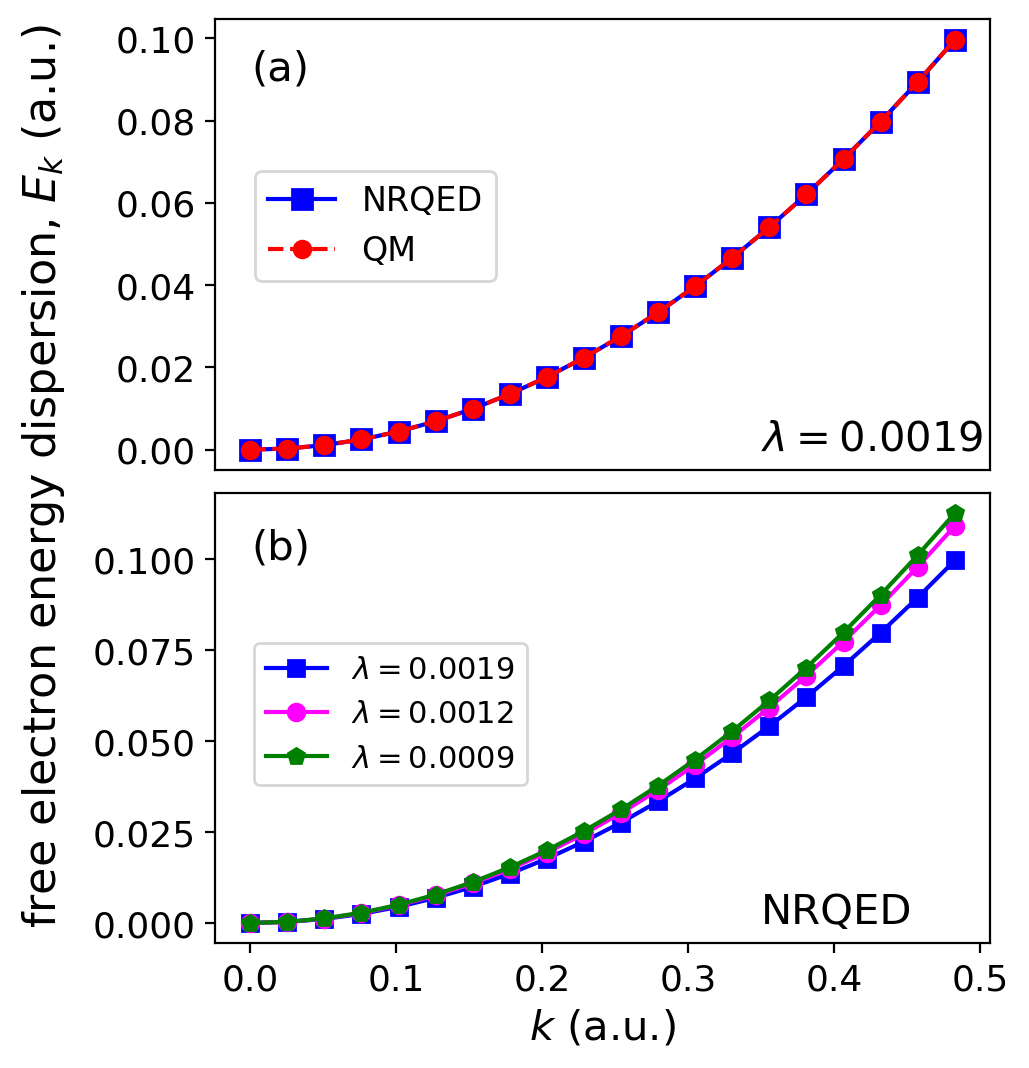
Figure 1: (a) The energy dispersion of a free electron in the NRQED setting when coupled to 200 photon modes and the corresponding QM case where the renormalized mass $m_{e}$ is used. Both settings show a quantitative agreement and we note this holds for different coupling strengths. (b) A comparison of the energy dispersion of NRQED for different $\lambda$’s where the dispersion relation is less confined for increasing $\lambda$.

Now, we will consider a situation of a free electron restricted to one dimension interacting with a discretized electromagnetic continuum. From this model, we want to demonstrate the working principles of the mass renormalization procedure and from this, obtain the observable mass of the interacting light-matter system in our corresponding quantum mechanics model. We will consider only the photon modes with polarization along the dimension the free particle is allowed to move. We choose the discretized photon continuum such that the range of its frequencies cover the desired energy range of the free electron and bound matter systems (discussed in Sec. IV). In this case, we introduce a lower and upper energy cutoffs which are respectively, 0.01 a.u. and 0.5 a.u. The upper cutoff is well within the validity of the dipole approximation. The lower cutoff is needed to treat the matter and the light sector consistently. Although non-perturbative NRQED has no infra-red divergence Spohn (2004), the consistent treatment of the $\omega\rightarrow 0$ needs extra care and we discuss this in a little more detail at the end of this section. Here we choose the lower cutoff in agreement with the matter grid by having $l=2\pi/k_{min}$. We sample the one-dimensional electromagnetic continuum by including explicitly 200 photon modes with equidistant energy spacing per mode of 0.00246 a.u. (see App. A for details on the photon continuum). This specified continuum of modes describes the local photonic density of states that we consider for the light-matter coupled system. In this setting of the coupled light-matter system, we compute the dispersion relations of Eq. (6), what we term as results from non-relativistic quantum electrodynamics (NRQED), and the dispersion relations of Eq. (7), what we call results from quantum mechanics (QM).

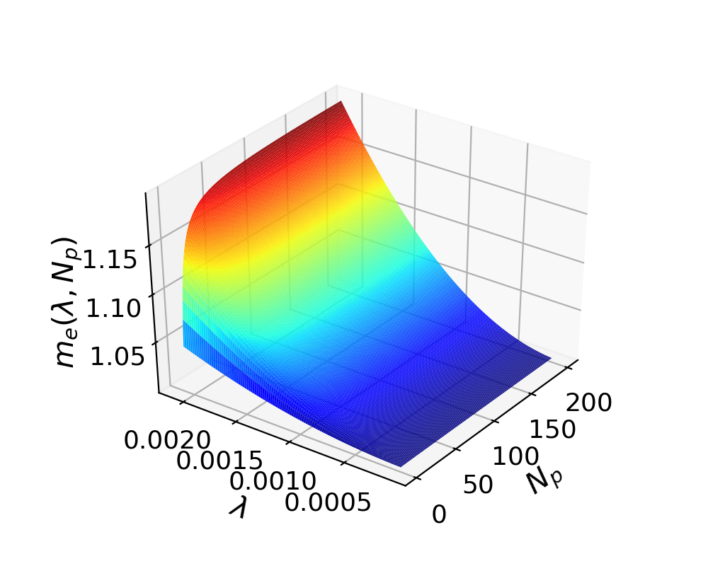
Figure 2: The dependence of the renormalized mass on the coupling parameter $\lambda$ and number of photon modes $N_{p}$. For fixed coupling and increasing number of modes the mass slowly diverges. For fixed number of modes and increasing coupling, the mass is shown to increase.

To obtain the dispersion relation of the QM setting requires that we perform a mass renormalization which accounts for the interaction between the free electron and the photon continuum. This procedure involves computing the observable mass as given in Eq. (8). In Fig. (1a), we show a comparison of the energy dispersion obtained from the NRQED and QM settings. We clearly find that the NRQED spectrum agrees quantitatively with the QM spectrum which highlights a clear connection between the non-relativistic QED and the quantum mechanics setting when the photonic degrees are traced out and included in the renormalized mass. The results at the same time demonstrates the validity and working principles of the mass renormalization procedure in the long-wavelength approximation. For the different coupling parameters $\lambda$, which for larger values indicate a stronger interaction with the photonic continuum, we find that the energy dispersion becomes less confined as shown in Fig. (1b). This is as a result of the photon-induced mass $m_{pt}$ as the free particle interacts with the photon field. Table (1) shows the physical masses for different $\lambda$ and from which the photon-induced mass $m_{pt}$ can be deduced according to Eq. (4).

Coupling parameter, $\lambda\;$	Renormalized mass, $m_{e}$
$0.0019$	$1.1683661411$
$0.0012$	$1.0673464565$
$0.0009$	$1.0336732282$

Table 1: The values of the renormalized mass $m_{e}$ obtained from Eq. (9) for different coupling strengths $\lambda$ when coupled to 200 photon modes. The value of the bare mass used is $m=1$.

In Fig. (2) we show how the observable mass depends on the coupling parameter $\lambda$ and the number of photon modes $N_{p}$ (i.e. increasing photonic density of states and energy cutoff). We find that for a fixed coupling (e.g., $\lambda=0.0020$) and increasing number of photon modes the observable mass increases and is expected to diverge when $g(N_{p})\rightarrow 1$ if the full continuum of photonic modes is spanned. On the other hand, for a fixed number of modes (e.g., $N_{p}=200$) and increasing coupling, the observable mass is shown to increase.

At this point it is important to highlight, that even in one dimension, the perturbative correction to the free-particle dispersion due the photon field is infrared divergent. The multimode coupling to second order perturbation theory has no upper bound (see Appendix B) and due to this, the perturbative correction becomes arbitrarily negative and leads to an instability as the particle dispersion from positive turns negative. Thus, perturbation theory violates the boundedness of the Pauli-Fierz Hamiltonian from below Spohn (2004); Rokaj et al. (2018). In contrast, the non-perturbative multimode coupling from the exact solution has an upper bound and it does not exceed unity, $g(N_{p})\leq 1$ (see Appendix B). Thus, the non-perturbative dispersion of the free particle is always positive and thus the system remains stable Rokaj et al. (2022b). This point highlights the importance of non-perturbative treatments of light-matter coupled systems. At the same time hints towards the idea proposed by Van Hove Van Hove (1952) that divergences in quantum field theory might be not be a generic propery but only due to perturbation theory.

Let us finally remark on the lower (infrared) cutoff and the consistency between light and matter. As is clear from the gauge coupling prescription the fields are directly related to the matter wave functions Ruggenthaler et al. (2023). So the matter grid determines which modes are possible. While we here have considered free particles, and the size of $L$ is somewhat arbitrary, we aim at considering bound-state systems, for which the dipole approximation is designed for. So the size of the simulation box is chosen such that all the relevant observables for the bound-state are well converged. The free-space case is numerically very instructive to understand that a mismatch between light and matter basis set leads to unphysical results. For instance, allowing for modes that are much smaller in energy than the minimal momentum eigenstate of matter results in a wrong dispersion relation that becomes flat (see App. C for an example). This again shows that length-scales do matter in QED, even if in the mathematically exact theory no divergence is found for soft photons Spohn (2004).

IV The bound matter system coupled to the electromagnetic continuum

The previous section considered the case of a free charged particle interacting with a discretized continuum of isotropic photonic modes. We will now consider the case of a bound matter system interacting with the same discretized continuum of modes and investigate some effects the photon modes have on several physical properties of the coupled system. For our investigation of the bound system, we chose to work with the length form of the Pauli-Fierz Hamiltonian given by Eq. (2). A practical advantage of the length gauge Hamiltonian is that for a real-space description of the bound matter system, the spectrum converges faster as opposed to the velocity gauge due to the different bilinear light-matter interaction terms of the different gauges Han and Madsen (2010); Bandrauk et al. (2013). For this reason, we choose to work with the length gauge Hamiltonian in the following. It is crucial to mention that the relation between the bare mass $m$ and the observable mass $m_{e}$ is the same in both gauges. The energy dispersion of the free electron in the length-gauge has exactly the same form as the one obtained in the velocity gauge. We demonstrate this fact for the single particle case in App. C. At this point we would like to emphasize that to obtain the free particle dispersion in the length-gauge the dipole self-energy is absolutely crucial. Without the dipole self-energy there is no translationally invariant direction in the electron-photon configuration space, i.e., translational invariance is broken Rokaj et al. (2018). As a consequence the free particle energy dispersion cannot be obtained at all. This makes evident the importance of the dipole self-energy for the mass renormalization procedure.

To obtain physical observables of the coupled light-matter system, we solve the stationary eigenvalue problem $\hat{H}|\Psi_{n}\rangle=E_{n}|\Psi_{n}\rangle$ of the Pauli-Fierz Hamiltonian of Eq. (2) and the quantum mechanics setting of Eq. (3) numerically exact and compare the results. In the QM setting for the bound systems, the contributions due to the interaction with a discretized continuum is accounted for by using the observbale mass obtained in Tab. (1) for the different couplings. We will consider two examples, the first being an atomic system and the other a molecular system that both interact with the electromagnetic continuum.

IV.1 The atomic light-matter system

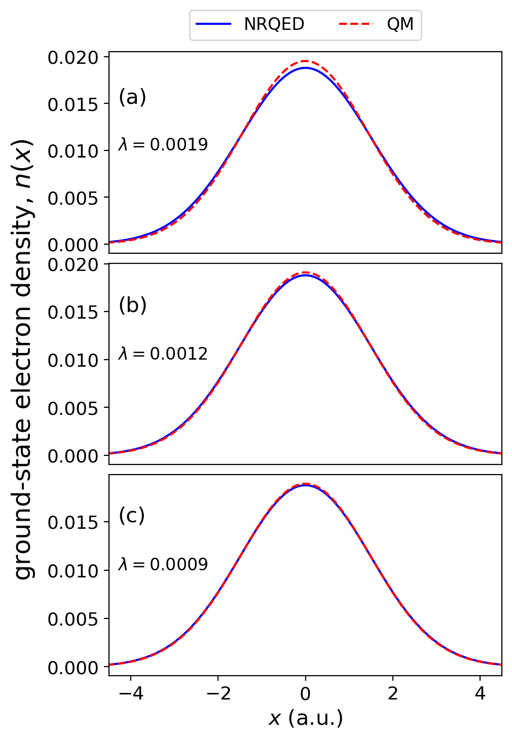
Figure 3: A comparison of the electronic ground-state density between between the NRQED and QM settings for a bound electron coupled to 200 photon modes. Panels (a-c) show the comparison for different coupling strengths $\lambda$ where the QM results deviate from NRQED due to how the bound system interacts with the descretized photonic continuum.

An important quantity of a matter system is the ground-state density as it describes the localization properties of matter. We investigate this property for the case of a one-dimensional atomic model (see App. D for the details of the model) coupled to the electromagnetic continuum. The atomic system interacts with the discretized continuum of photon modes discussed in Sec. III. For this setting of the coupled light-matter system, we compute the ground-state electron density and make a comparison between the NRQED and QM settings. In the setting of a bound system, we expect to obtain a good quantitative agreement between NRQED and QM as in the free electron case in Sec. III. However, we find that this is not the case as illustrated in Fig. (3) for the different light-matter coupling strengths. Instead, we find that the results from QM deviates from NRQED as the system in its ground-state becomes more bound as indicated by the increased amplitude and shrinking of the width of the density profile. In this setting of a bound system interacting with a continuum, it is interesting to find that the mass renormalization procedure that gives the QM setting does not agree with the NRQED results.

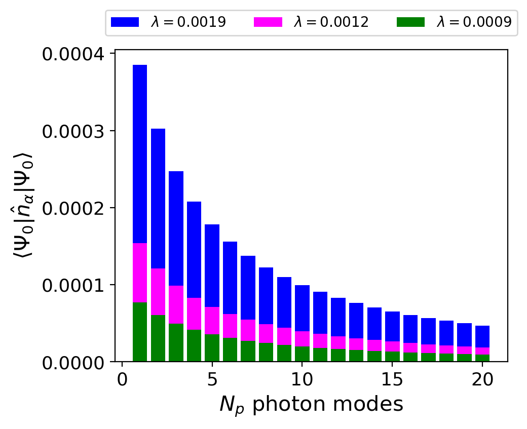
Figure 4: The photon occupation of the electron-photon ground-state for the atomic system coupled to a discretized continuum sampled with $N_{p}=200$ photon modes. Only the occupations of the first 20 low lying photon modes are shown where the lowest modes couple strongly and the occupation increases with the coupling strength. Each bar represents the contribution of each photon mode to the photon occupation.

The reason for this deviation is that by introducing a binding potential the localized electronic states do not couple equally to all the modes of the discretized electromagnetic continuum as opposed to the free space case studied above. Since the energy dispersion of Fig. (1) is actually an excited state property, it probes a larger part of the photonic continuum of modes. Hence, the resulting observable mass obtained from Eq. (8) (see values in Tab. (1)) includes a large contribution from the high-lying modes of the electromagnetic continuum. Therefore, using this renormalized mass in Eq. (3) leads to the deviations seen in Fig. (3). This is elucidated clearly in the second point were we illustrate how the different photon modes interact with the atomic system by computing the mean photon occupation per photon mode defined in the velocity gauge as $n_{\alpha}=\langle\Psi_{0}|\hat{n}_{\alpha}|\Psi_{0}\rangle$ where $\hat{n}_{\alpha}=\hat{a}_{\alpha}^{\dagger}\hat{a}_{\alpha}$ and $|\Psi_{0}\rangle$ is the correlated electron-photon ground-state. For different light-matter couplings $\lambda$, we show in Fig. (4) the mean photon occupation for the lowest lying 20 of the 200 photon modes. Clearly, the lower lying photon modes have more photon occupation as they interact more with the atomic system when compared to the high-lying modes. Also, we find that the stronger the coupling $\lambda$ the higher the photon occupation and the decreasing trend of photon occupation for higher lying photon frequencies applies for the different $\lambda$’s. From these results we can deduce that ground-state properties will saturate with increasing photon modes with higher frequencies (i.e., increasing photonic cutoff).

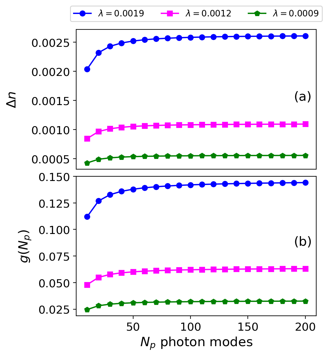
Figure 5: (a) The integrated ground-state density difference $\Delta n$ between the NRQED and QM settings when coupled to different photon modes in the range 10 to 200 and increasing coupling $\lambda$. (b) The dependence of the multimode mode coupling on the photon number of photon modes for different light-matter coupling.

To demonstrate this, we compute the integrated ground-state electron density difference defined as $\Delta n=\int dx|n(x)-n^{\prime}(x)|$ where $n(x)$ and $n^{\prime}(x)$ are the densities of two different settings. Since NRQED is the reference result, we compute this quantity for NRQED and QM for increasing number of modes (increasing cutoff) from 10 to 200 modes in steps of 10 modes and increasing coupling $\lambda$. This comparison is shown in Fig. (5a) where we find that “NRQED$-$QM” (density of NRQED minus QM) saturate for increasing photon modes for the different couplings. From the results of Figs. (3) and (5a), we also infer that the atomic system becomes more bound (increased localization) for increasing photon modes (photonic cutoff energy). A conclusion that can be drawn from the results of Figs. (4) and (5a) is that for the bound system not all photon modes are equally important since the effect of coupling to the ground-state becomes smaller for higher photon frequencies. This implies that the bound system saturates faster than the free particle as a function of the number of modes $N_{p}$. It is interesting to highlight that the multimode coupling $g(N_{p})$ for different light-matter coupling have a similar dependence on the number of photon modes as the integrated ground-state density up to a multiplicative prefactor as shown in Fig. (5b). We would like to mention that the enhanced localization as a result of mass renormalization, has been reported even with a single cavity mode for a many-particle system in a harmonic trap Rokaj et al. (2023b). In this case the localization phenomenon was significantly enhanced due to the collective coupling of the system and cavity-mediated interactions. A further important point to make here is that, as opposed to the free-space case, where Eq. (9) shows that a finite cutoff/regularization needs to be kept, for ground states, even in the long-wavelength approximation NRQED might be cutoff-independent for a fixed bare mass value.

IV.1.1 Impact of Mass Renormalization on excited-state properties

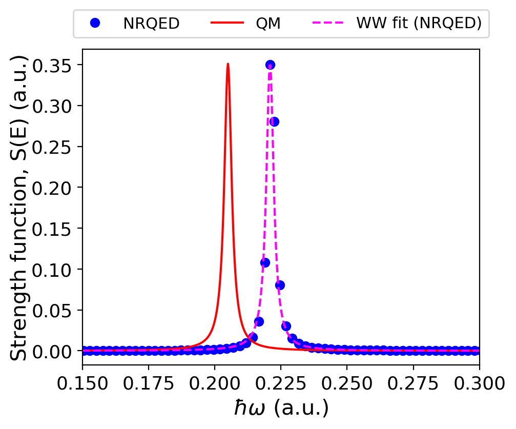
Figure 6: The absorption spectrum of the NRQED setting without applying an artificial broadening and the corresponding fitted spectrum with Wigner-Weisskopf (WW) theory (magenta) with a Lorentzian broadening of $\hbar\gamma=0.0034$ a.u. The same broadening and WW theory is employed to obtain the absorption spectrum of the QM setting (red).

We have so far considered only ground-state properties for the atomic system interacting with the discretized electromagnetic continuum. Now, we focus on excited-state properties of this coupled system. One common quantity which is normally computed is the absorption spectrum of the system which we determined here by computing the dipole strength function $S(\omega)=\sum_{n}2\omega_{n}|\langle\Psi_{0}|\hat{x}|\Psi_{n}\rangle|^{2}\delta(\omega-\omega_{n})$ where $\hat{x}$ is the electronic dipole operator of the one-dimensional atomic system. For this quantity, we make a comparison for the different settings of NRQED and QM as shown in Fig. (6) where we employ Wigner-Weisskopf theory to fit the NRQED results and subsequently obtain the spectrum of the QM setting. Similar to the ground-state results, we find that the QM deviates from NRQED in peak position. The reason for this can be partly attributed to how the discretized continuum of modes interact with the atomic system and affect ground-state properties such that a transition from the ground-state to the first excited state leads to this deviation. We expect that for higher-lying excitations in the absorption spectrum, the NRQED and QM settings should agree since the excited states become more delocalized and should probe a large part of the continuum as in the free electron case discussed above. A noticeable difference is that the absorption peak of QM is red-shifted in the spectrum relative to NRQED. From the analytic expression of the energies of the atomic system given in Eq. (28), we deduce that for a larger mass (i.e. the observable mass), the energies become more negative (strongly bound) which causes the red shift relative to NRQED peak. In passing, we note that for a more dense sampling of the discretized continuum of modes as done in Refs. Flick et al. (2019); Welakuh et al. (2022); Welakuh and Narang (2022b), we will obtain a smooth Lorenztian profile for the NRQED case that naturally occurs due to the continuum of modes.

IV.2 The molecular light-matter system

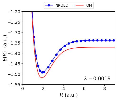
Figure 7: A comparison of the ground-state PoPESs showing a deviation between the QM and NRQED results. The PoPES for NRQED is the case when coupled to 50 photon modes and QM uses the observable mass due to the same photonic density of states.

We now investigate how molecular properties are affected when a molecular system interacts with the discretized continuum of photon modes. As a molecular system, we consider a one-dimensional model of a hydrogen molecule (see App. E for details) that interacts with the discretized continuum of photon modes discussed in Sec. III. For the calculations of the molecular light-matter system, we couple the molecule to the lowest 50 photon modes since they are the most important for bound systems as discussed above. A common and widely studied property of a molecule is its potential energy surface (PES) which describes the relationship between the molecular geometry, for example, the relative positions of the participating atoms, and the molecular energy. For the case of coupled light-matter systems we have similar objects. Since we have three natural subsystems, i.e., nuclei, electrons and photons, we can perform the Born-Huang expansion that underlies the PES concept in different ways. In our case, where the frequency range is chosen to affect the electronic degrees of freedom (as we show in the SI, the basic frequency of the nuclear degrees of freedom is $\omega_{e}\approx 0.02$ a.u. which is within the lower frequencies of the sampled continuum), we can use a grouping of the photonic degrees of freedom with the electronic ones. This leads to polaritonic PES (PoPES) Feist and Garcia-Vidal (2015), where the nuclei (in our case indicated by the internuclear separation $R$) feel the photonic continuum of modes via the changes in the PoPES.

We now show in Fig. (7) the ground-state PoPES for the different settings, were the QM result deviates from the NRQED result. This result is similar to the atomic light-matter system discussed above were the lower-lying modes of the continuum couple strongly compared to the higher-lying modes which causes the deviation when the calculated renormalized mass (in Tab. (1)) is used in the QM setting. To support this, we show in Fig. (17) that the ground-state density of NRQED and QM, were we find that the QM result shows that the molecular system at the equilibrium position becomes more bound compared to the NRQED result similar to the atomic light-matter results in Fig. (3a). We note that we have removed the vacuum contribution of the zero-point energy due to the 50 photon modes from the PoPES of NRQED. That means, we have normal-ordered and discarded an overall constant energy contribution.

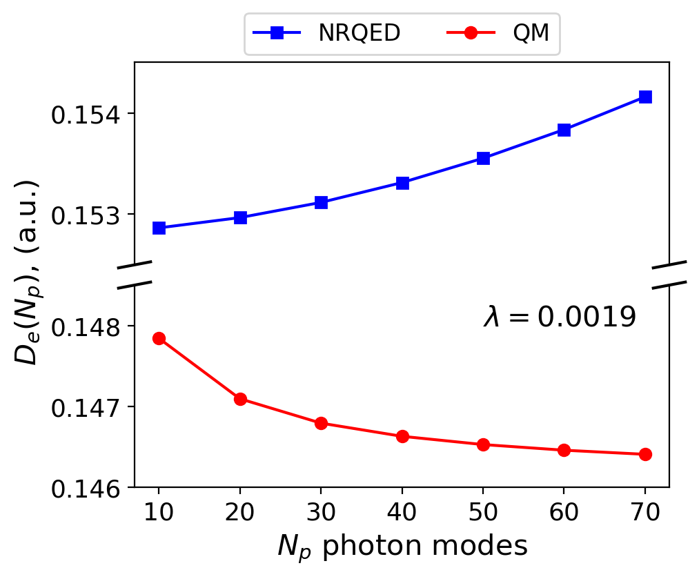
Figure 8: The photon-mode-dependent dissociation energy plotted as function of photon modes for the NRQED and QM settings. The NRQED setting indicates that it is increasing difficult to break a bond for increasing $N_{p}$ while QM shows the opposite behavior.

Another important information that can be obtained from Fig. (7) is the bond dissociation energy $D_{e}$ of the molecule. The results on how the dissociation energy of the H₂ molecule changes with increasing photonic energy cutoff (number of photon modes) is shown in Fig. (8). For up to 70 photon modes, the photon-mode-dependent dissociation energy for NRQED and QM has an opposite behavior. For NRQED the dissociation energy increases with increasing energy cutoff which implies that it is more difficult to break a chemical bond when the molecule is made to interact strongly with the electromagnetic continuum while QM shows the opposite behavior. Just as in the atomic light-matter system, a similar conclusion can be drawn for the molecular case were we note that not all photon modes are equally important. Thus, the effect of coupling to the ground-state becomes smaller for higher photon frequencies which leads to differences with the QM setting due to the renormalized mass obtained from the free electron light-matter setting.

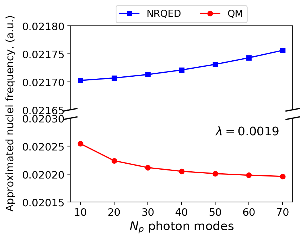
Figure 9: A comparison of the harmonic-approximated frequency of the ground-state PoPES between NRQED and QM as a function of the number of photon modes $N_{p}$. The approximated harmonic frequency for $N_{p}=0$ is $\omega_{e}=0.020455$ a.u.

As we have seen, the PoPES is changed due to the interaction with the photon modes. To quantify the effect of the modes on the nuclear degrees further we next consider the change in vibrational frequencies in the $H_{2}$ molecule. Since we have chosen a Born-Huang grouping of the electrons with the photons, the effect of the many modes is mediated via the changes in the PoPES. We note that for free interacting protons coupled to the electromagnetic continuum, we obtain an analogous dispersion energy as in Eq. (6) with a diamagnetic frequency that is dependent on the nuclear charge. From the energy dispersion the renormalized proton mass can be obtained and with this we can investigate how the nuclear degrees are influenced due to coupling to the electromagnetic continuum in a QM setting. In Fig. (9) we show the results of the harmonic-approximated vibrational frequency dependence on the sampled photon continuum (see App. F for details). We find for NRQED that the approximate harmonic vibrational frequency increases with the number of photon modes indicating that the nuclear degrees of the ground-state PoPES becomes more bound while the QM setting shows the opposite behavior. The behavior of the approximate harmonic frequency is reminiscent of the dissociation energy in Fig. (8) since it is proportional to the square-root of $D_{e}$. We can thus conclude that the nuclear degrees of freedom are influenced in a similar way to the electronic degrees where only the lower-lying photon modes play a significant role.

In addition, the fact that the PES of the $H_{2}$ molecule is modified indicates that the photon field modifies the long-range interactions between the atomic dimer. The intuition that the mediated forces are of long-range nature is due to the fact that if we fit the PESs, with and without coupling to the photon field, we find that the defining parameters ($D_{e},a,\textrm{and}\;\omega_{e}$) of the Morse model are modified when the molecule is coupled to light. The Morse model effectively describes the long-range interactions between the pair of atoms, which are responsible for the formation of the molecule. Thus, it becomes evident that the photon field makes an impact on these long-range interactions.

IV.3 Cavity-modifications of the ground state

In this section we focus on how enhancing the coupling between the bound matter system and the electromagnetic continuum can lead to the modification of ground-state properties. There are several methods by which the coupling to the electromagnetic continuum can be enhanced, e.g., using a planar cavity as a photonic structure. Here, we distinguish two settings how the discretized photon continuum interacts with matter. The first setting is the reference “free-space” case were the discretized continuum is weakly coupled to matter and we chose $\lambda=0.0009$ to designate the free-space coupling. In the second setting, the discretized continuum can be made to strongly interact with matter as realized within planar optical cavities by decreasing the mode volume to enhance the coupling. In this cavity setup, we enhance the coupling to the discretized continuum by increasing the coupling parameter $\lambda=0.0012,0.0019$. As we learned from the Sec. III, we need to have the matter and the photonic degrees of freedom to be consistent. We therefore only consider the photonic density of states in the relevant frequency range, where there are matter states that can be affected by the photons. We do not consider how the photonic density of states is changed outside of this frequency range, from where the extra density of states is taken from. We will investigate the properties only in the NRQED setting.

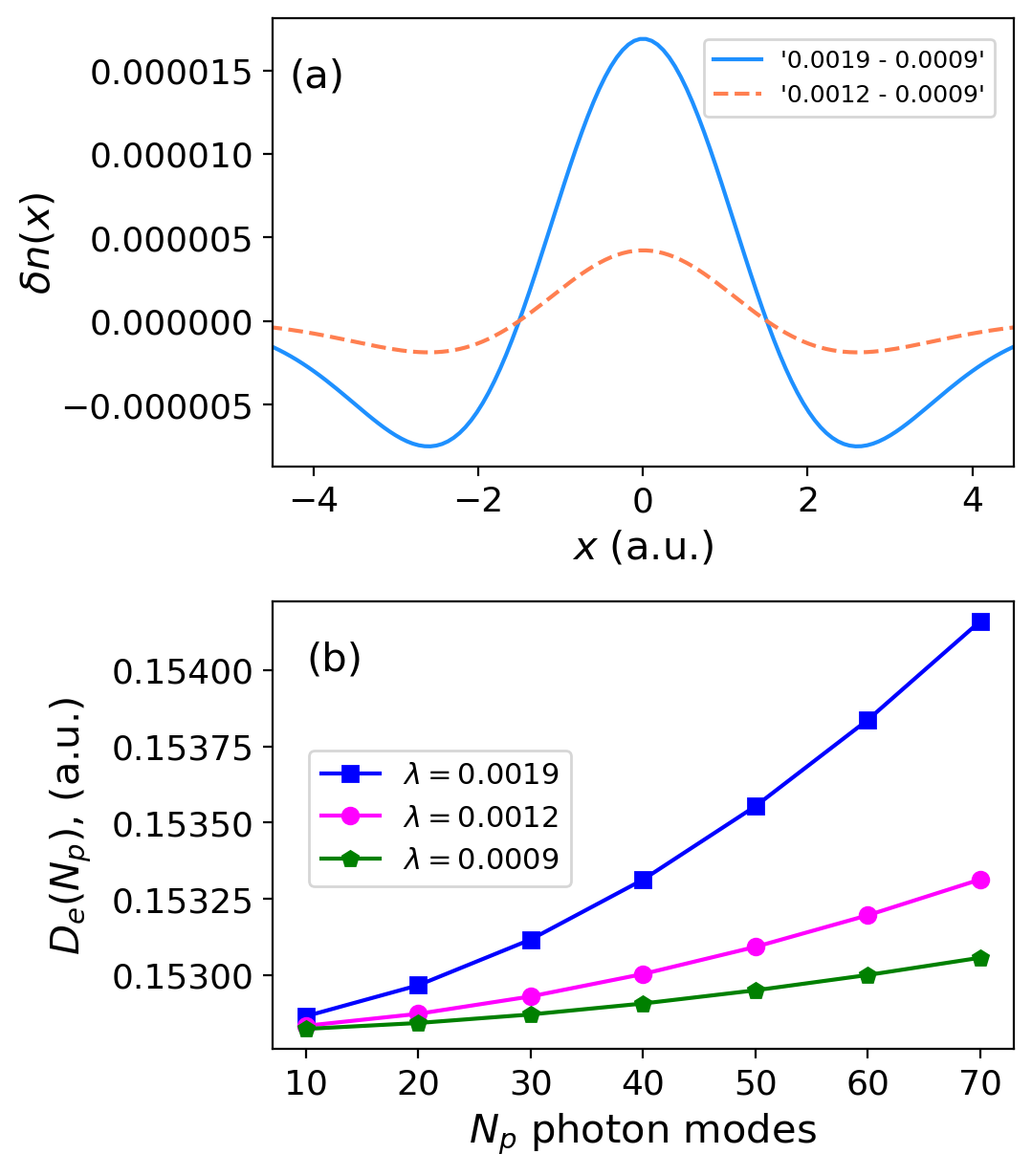
Figure 10: (a) The ground-state density difference $\delta n(x)$ between the cavity and free space case for two cases (blue: “$0.0019-0.0009$”) and (orange: “$0.0012-0.0009$”). (b) A comparison of the photon-mode-dependnet dissociation energy for different light-matter coupling.

In Fig. (10), we show the results of the atomic and molecular light-matter systems for the free space and the cavity settings. For the atomic system in Fig. (10a), we compute the difference between the ground-state density $\delta n(x)$ of the free space case ($\lambda=0.0009$) and when we enhance the coupling to the discretized continuum with cavity with couplings ($\lambda=0.0012,0.0019$). Although relatively small, we find that there are cavity-induced modifications of the ground-state density (i.e. atomic system is more bound) when we change the photonic continuum using a cavity. For the molecular light-matter in Fig. (10b), we show the photon-mode-dependent dissociation energy of the ground-state PoPES where we find that it becomes more difficult to break a chemical bond when the cavity mode enhances the coupling to discretized continuum. These results highlights that ground-state properties of bound systems can be modified when the coupling to the photonic continuum is enhanced, for example, using an optical cavity.

V Approximation strategies for multi-mode ground-state modifications

The effects that we have found for our simple models are expected to arise in realistic systems when the electromagnetic continuum of modes interact with a bound matter system. A non-perturbative simulation of this setting becomes computationally demanding especially when including explicitly the electromagnetic continuum. Here, we present different ways to capture approximately the effects that arises due to the coupling to the continuum which can be considered a prerequisite for making relevant predictions in practice.

V.1 Quantum mechanics with a self-polarization contribution

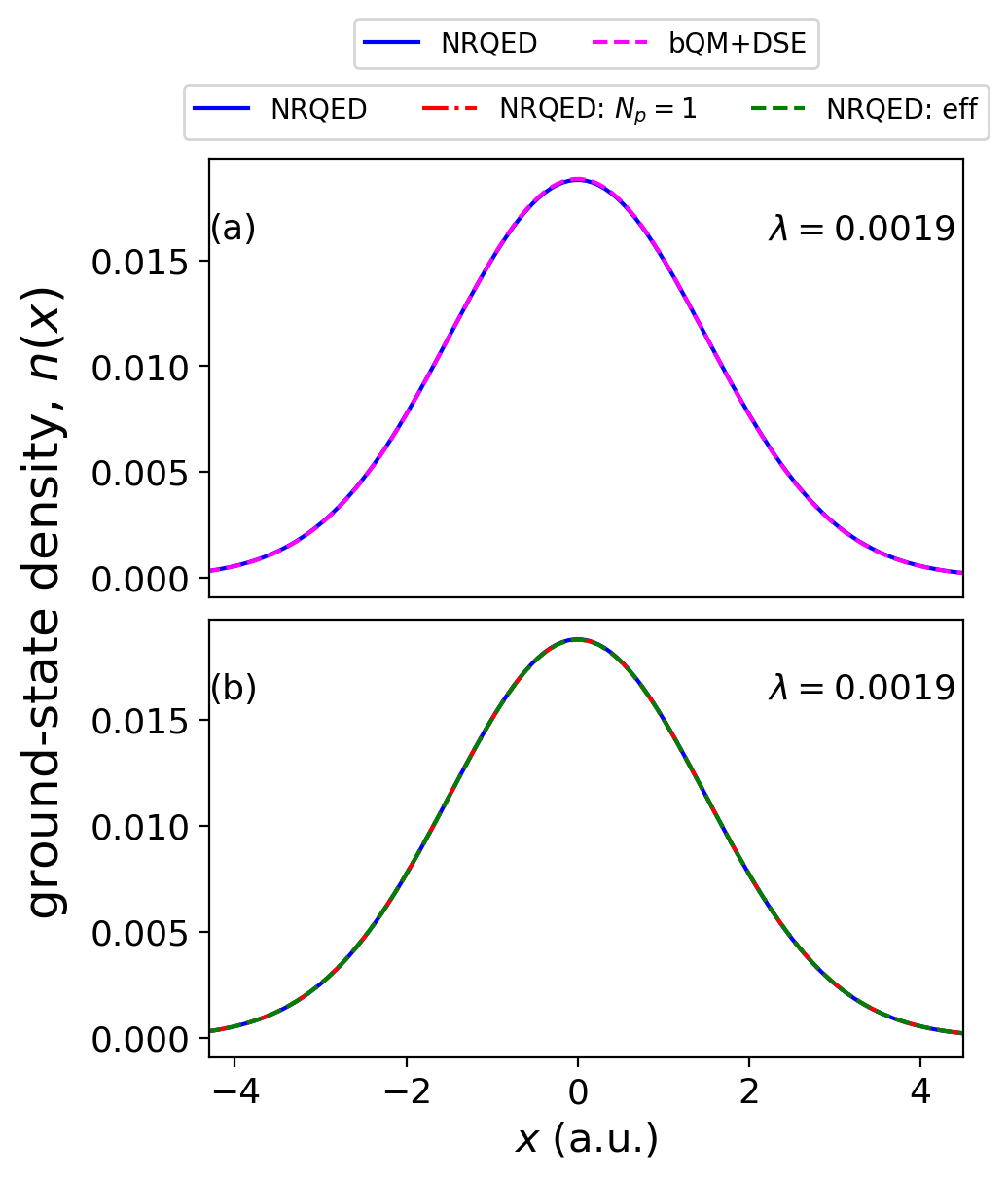
Figure 11: (a) The ground-state electron density of the atomic system for NRQED compared to that of the bQM$+$DSE approximation when coupled to 200 photon modes. The results are quantitatively the same with $\Delta n=1.8\times 10^{-5}$. (b) A similar quantitative agreement between NRQED and the single mode approximations for the atomic ground-state density.

In the first approach, the approximation is applied to the length gauge Hamiltonian by keeping only the self-polarization term of the transverse contributions of the Hamiltonian. As we will show, this is particularly valid for ground-state properties of the coupled system, were we can drop the bilinear light-matter interaction term since for the most part, it affects more the excited state properties of the coupled system. In this approximation, we will drop all the terms of Eq. (2) that have explicit dependence on the displacement coordinate $\hat{q}_{\alpha}$ and conjugate momentum $\hat{p}_{\alpha}$ to obtain the bare quantum mechanics including the dipole-self energy (bQM$+$DSE) Hamiltonian given as follows

$$\hat{H}_{\text{bQM+DSE}} =\hat{H}_{\text{bQM}}+\frac{1}{2}\sum_{\alpha=1}^{N_{p}}\left(\boldsymbol{\lambda}_{\alpha}\cdot\hat{\boldsymbol{\mu}}\right)^{2},$$ (10)

where the transversal contribution from the electromagnetic field are only accounted for using the dipole self-polarization term (last term of Eq. (10). Here, we denote the $\hat{H}_{\text{bQM}}$ the bare quantum mechanics Hamiltonian where the bare mass is used instead of the renormalized mass since we are still coupling to the electromagnetic field via the DSE term. This approximation becomes reasonable once we have $\langle\boldsymbol{\lambda}_{\alpha}\cdot\hat{\boldsymbol{\mu}}\rangle=0$ and thus due to the zero field condition also $\langle\hat{q}_{\alpha}\rangle=0$. Else we need to keep the contributions of the displacement field to exactly cancel the polarization field Flick and Narang (2018); Schäfer et al. (2020). We will apply this approximation to the bound light-matter systems where in the case of the atomic system, we compare the electronic ground-state density from the NRQED setting to the bQM$+$DSE. For the molecular system, we compare the ground-state PES from the NRQED to the bQM$+$DSE settings.

For the atomic light-matter system, we show in Fig. (11a) a comparison of the results obtained for the ground-state electron densities of NRQED and bQM$+$DSE when the atomic system is coupled to 200 photon modes. We find that on the plotted scale, they are quantitatively the same and we obtain an integrated ground-state density difference between the two cases of $\Delta n=1.8\times 10^{-5}$. When we vary the photon modes included in the computation of the ground-state, we obtain a result that is quantitatively the same to the red plot of Fig. (5). This result demonstrates that including the transversal contribution of the electromagnetic field only with DSE term is capable of describing the ground-state properties in non-resonant light-matter interactions. Next, for the molecular light-matter system we consider the case when the molecule is coupled to the lowest 50 of the 200 photon modes. In Fig. (12a) we show a comparison between the ground-state PES of the bQM$+$DSE and NRQED where both are shown to agree quantitatively. The result demonstrates that the bQM$+$DSE approximation is sufficient for describing also molecular light-matter properties in the ground-state of the coupled system.

V.2 Effective Single Mode Description

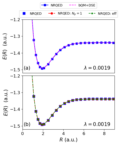
Figure 12: (a) The ground-state PES when coupled to 50 photon modes for NRQED which agrees quantitatively with the bQM$+$DSE approximation. (b) A comparison of the same NRQED ground-state PES to the effective one mode approximations with the same quantitative agreement.

In the second approach, the approximation we describe is widely applied in polaritonic chemistry and cavity quantum materials Schlawin et al. (2022); Ebbesen (2016); Garcia-Vidal et al. (2021), were we make the usual assumption that we can describe the multimode cavity by one effective photon mode. After making this approximation, one usually computes ground-state or excited-state properties of the strongly coupled light-matter system. Here, we will apply such an approximation in two different ways. For the first approach, we select only one of the 200 photon modes and couple to the bound system as described by Eq. (2). Out of the 200 modes, we choose the $N_{p}\!=\!1$, i.e., the lowest frequency mode with cavity frequency $\omega_{\alpha=1}\!=\!0.01$ a.u. and coupling $\lambda=0.0019$ which is the strongly coupled mode as shown in Fig. (4). In the second approach, we take an average of the entire sampled photon modes to obtain one effective mode. For example, the case were 200 modes are sampled, the effective cavity frequency is $\omega_{\text{eff}}\!=\!0.255$ a.u. and the corresponding average over the light-matter parameter is $\lambda=\lambda_{\text{eff}}=0.0019$. For the atomic system, we look at ground-state properties of the two approaches by computing the electronic ground-state density of the atomic system and for the molecular system we look at the dissociation energy of the ground-state PES.

Starting with the atomic light-matter system, in Fig. (12b) we show for the ground-state density how the two approaches compare to the NRQED including 200 photon modes. We find that the (NRQED: $N_{p}=1$) and (NRQED: eff) are quantitatively the same when compared to NRQED. Also, for the molecular light-matter interacting system, we find in Fig. (11b) the same quantitative agreement for both single mode approximation when compared to the ground-state PES of NRQED. These results demonstrate that modeling the multi-mode cavity with one effective mode can capture ground-state effects of a multi-mode photonic cavity which is of practical importance when working with realistic systems interacting with a continuum of modes.

VI Summary, Conclusion and Outlook

We have investigated non-perturbatively how the coupling to a continuum of modes leads to mass-renormalization effects in ab initio QED. Starting with the free charged particles interacting with a photonic continuum of modes, we demonstrated the free-space mass renormalization procedure and highlighted how it connects two levels of theory (QM and NRQED) by the energy dispersion. We showed how the experimentally observable mass depends on the number of photon modes (local photonic density of states) and increasing light-matter interaction strength. For a non-perturbative mass renormalization of a bound system coupled to light, we found that the NRQED and QM settings do not agree for both its equilibrium and excited-state properties. This occurs because the bound system interacts differently with the electromagnetic continuum as opposed to the free particle case. That is, out of the sampled discretized continuum only a few of the lowest lying photon modes play a significant role when interacting with a bound system. Finally, we demonstrated how approximations like the effective few-mode or dipole-self-energy approximation can capture non-trivial ground-state effects. Specifically, we showed for the ground-state density and PES of the respective atomic and molecular systems quantitative agreements with the numerically exact results. While these considerations were restricted to simple one-dimensional model of NRQED, we expect that similar mass-renormalization effects are ubiquitous in light-matter interactions. Understanding these inherently non-perturbative effects could help us to get a further theoretical control-knob on the properties of matter in photonic environments. Besides this more practically relevant implications, the obtained theoretical insights could provide a different viewpoint on the renormalization effects that show up in interacting quantum field theories.

In this work we have considered a simple one-dimensional model setup of NRQED. Naturally the question arises, whether similar effects will be found in real three dimensional ab initio systems. Based on the previous section, where we have shown that one can recover qualitatively similar results with simple bQM$+$DSE or single-mode approximations, it seems obvious that these effects will be found also for realistic systems. The bQM$+$DSE and few-mode simulations can nowadays be done routinely Flick et al. (2019). The main difference when going to three dimensions will be the anisotropy of the renormalized masses. The cavity breaks the simple free-space symmetries and it will be interesting how these symmetry-breaking can influence real systems. The renormalization effects will also change if we go beyond the long-wavelength approximation. Although in free-space there is a fundamental difference between minimal-coupling and the long-wavelength approximation, i.e., dipole approximation is not non-perturbatively renormalizable and for the full Pauli-Fierz Hamiltonian it might be possible similar to the Nelson model Spohn (2004); Hiroshima and Spohn (2005), the saturation effect for bound states might point towards a very similar behavior of the long-wavelength and the minimal-coupling situation. Also, based on the success of the dipole approximation for bound systems, it seems reasonable to assume that in such cases the differences are commonly small. Clearly, there are many cases where one expects stark differences, such as due to self-organization in a cavity or when large momenta are transferred between light and matter. Overall we believe, however, that the obtained model results are a very good indicator when similar effects will appear in real ab initio systems.

Appendix A Numerical Details

We outline the numerical details to treat the coupled matter-photon system. First, for the matter Hamiltonian of the one-dimensional atomic system, we represent the single bound electron on a uniform real-space grid of $N_{x}=3000$ grid points with grid spacing $\Delta x=0.0707$ a.u. while applying an eighth-order finite-difference scheme for the momentum operator and Laplacian. Next, we perform an exact diagonalization of the Hamiltonian and obtain the spectrum of the system (converged eigen-energies $E_{i}$ and eigen-states $|\psi_{i}\rangle$). Now, using the completeness relation $\sum_{i=1}^{\infty}|\psi_{i}\rangle\langle\psi_{i}|=\hat{\mathbb{1}}$, the operators of the matter system can be expressed as Loudon (2000)

$$\hat{H}_{\text{M}} =\sum_{i=1}E_{i}|\psi_{i}\rangle\langle\psi_{i}|,\;\;\hat{\textbf{p}}=\sum_{i=1}\sum_{j=1}\langle\psi_{i}|\hat{\textbf{p}}|\psi_{j}\rangle|\psi_{i}\rangle\langle\psi_{j}|,\;$$

$$\hat{\textbf{R}} =\sum_{i=1}\sum_{j=1}\langle\psi_{i}|\hat{\textbf{R}}|\psi_{j}\rangle|\psi_{i}\rangle\langle\psi_{j}|,$$

where the indices $i,j$ runs over the number of matter states considered. We consider $N_{s}=10$ lowest energy states to couple to the electromagnetic field. For the photonic subsystem, each photon mode is represented in a basis of Fock number states. In order to be able to treat the discretized photonic continuum numerically exact, we sample $N_{p}=200$ photon modes where we truncate the Fock space and consider only the vacuum state, the $N_{p}$ one-photon states, and the $(N_{p}^{2}+N_{p})/2$ two-photon states as in Ref. Flick et al. (2017). This implies the dimension of the photonic continuum is $1+N_{p}+(N_{p}^{2}+N_{p})/2=20301$. Coupling to $N_{s}=10$ lowest energy states of the atomic system give a matter-photon dimension of $10\times 20301=203010$.

For the hydrogen molecule (H₂) in 1D, we used a grid $(0,9]$ au for the internuclear separation with a uniform grid spacing $\Delta R=0.1$ a.u. For the electron coordinates ($\hat{x}_{1}$ and $\hat{x}_{2}$), we represent both electrons on a uniform real-space grid of $N_{x_{1}}=N_{x_{2}}=200$ grid points with grid spacing $\Delta x_{1}=\Delta x_{2}=0.35$ a.u. We perform exact numerical diagonalizations to obtain the spectrum. We couple to the discrete photonic continuum as described above.

Appendix B Perturbative and Exact Free Particle Dispersion and Continuum Behaviors

In this section we compute the free particle dispersion in 1D perturbatively and we compare to the exact non-perturbative solution. Following Ref. Craig and Thirunamachandran (1998) the first non-trivial correction to the free particle dispersion in three dimensions is

$$\Delta E=\frac{e^{2}}{m^{2}}\sum_{\mathbf{p}^{\prime},\mathbf{k},\alpha}\frac{\hbar\mathbf{e}_{\alpha}(\mathbf{k})\cdot\mathbf{e}_{\alpha}(\mathbf{k})}{2\epsilon_{0}c|\mathbf{k}|V}\frac{\langle\phi_{\mathbf{p}}|p_{i}|\phi_{\mathbf{p}^{\prime}}\rangle\langle\phi_{\mathbf{p}^{\prime}}|p_{j}|\phi_{\mathbf{p}}\rangle}{\mathbf{p}^{2}/2m-\mathbf{p^{\prime}}^{2}/2m-\hbar c|\mathbf{k}|}.$$

In our effective one-dimensional model the polarization vectors are all parallel and the correction to the energy dispersion simplifies

$$\Delta E=\frac{e^{2}}{m^{2}}\sum_{p^{\prime},k}\frac{\hbar}{2\epsilon_{0}c|k|V}\frac{\langle\phi_{p}|p|\phi_{p^{\prime}}\rangle\langle\phi_{p^{\prime}}|p|\phi_{p}\rangle}{p^{2}/2m-{p^{\prime}}^{2}/2m-\hbar c|k|}\,.$$ (12)

Then, we use the property for the plane waves $\langle\phi_{p}|p|\phi_{p^{\prime}}\rangle=p\delta_{pp^{\prime}}$, we sum over $p^{\prime}$ and we find

$$\Delta E=-p^{2}\frac{e^{2}}{m^{2}c^{2}}\frac{1}{2\epsilon_{0}V}\sum_{k}\frac{1}{k^{2}}\,.$$ (13)

To perform then the summation over all photonic momenta $k$ we promote the sum into an integral by taking the thermodynamic limit. For this purpose we write the mode volume as $V=AL$ and we have

$$\Delta E=-p^{2}\frac{e^{2}}{m^{2}c^{2}}\frac{1}{4\pi\epsilon_{0}A}\int^{\Lambda_{u}}_{\Lambda_{l}}\frac{dk}{k^{2}}\,,$$ (14)

where $\Lambda_{u}$ and $\Lambda_{l}$ are the limits of integration. After the integration we find

$$\Delta E=-\frac{p^{2}}{2m}\frac{e^{2}}{2m\pi\epsilon_{0}A}\left(\frac{1}{\Lambda_{l}}-\frac{1}{\Lambda_{u}}\right)=-\frac{p^{2}}{2m}g(\Lambda_{u},\Lambda_{l}).$$

From the expression of the multimode coupling constant $g(\Lambda_{u},\Lambda_{l})$ it is clear that the perturbative correction is not divergent in the ultraviolet (UV) since the limit $\Lambda_{u}\rightarrow\infty$ can be taken safely and the term $1/\Lambda_{u}$ goes to zero. This can be understood from Fig. 13 where we plot the perturbative coupling $g(\Lambda_{u},\Lambda_{l})$ normalized by the prefactor $e^{2}/2m\pi\epsilon_{0}A$ and for a fixed lower cutoff $\Lambda_{l}$. The coupling constant increases rapidly and asymptotically reaches a fixed value which is $\frac{e^{2}}{2m\pi\epsilon_{0}A}\frac{1}{\Lambda_{l}}$ which means that the perturbative multimode coupling converges with the UV cutoff $\Lambda_{u}$. However, the perturbative coupling diverges if the lower cutoff is taken to zero,

$$\lim_{\Lambda_{l}\to 0}g(\Lambda_{u},\Lambda_{l})\rightarrow\infty\,.$$ (16)

This implies that the perturbative coupling is divergent in the infrared (IR) part of the electromagnetic spectrum. As a consequence the perturbative correction to the free particle dispersion $\Delta E$ becomes arbitrarily negative and thus the perturbative computation leads to an instability as the particle dispersion from positive turns negative. Thus, perturbation theory violates the boundedness of the Pauli-Fierz Hamiltonian from below and the perturbative free particle spectrum no longer has a minimum.

In contrast to the perturbative computation, the physical picture emerging from the non-perturbative solution of the free particle is different Rokaj et al. (2022b). In Fig. 14 we plot the exact non-perturbative multimode coupling constant $g(N_{p})$ as a function of the number of photon modes $N_{p}$ as given from Eq. (6). We see that $g(N_{p})$ has effectively the same dependence with respect to the amount of photon modes as the perturbative coupling $g(\Lambda_{u},\Lambda_{l})$ with respect to the upper cutoff $\Lambda_{u}$. They both increase rapidly and then reach a plateau. However, with the respect to the lower photonic cutoff their behaviors are drastically different. The non-perturbative coupling constant $g(N_{p})$ has an upper bound and never exceeds 1, even for very large values of the ratio $\omega_{d}/\omega=10,15$. We note that $\omega$ here denotes the lowest frequency considered in the photonic spectrum. From Fig. 14 it is clear that if we fix $\omega_{d}$ then for arbitrarily small $\omega$ the multimode coupling can reach unity but never exceeds it. In contrast to the perturbative coupling, the exact coupling never diverges and as consequence the free particle dispersion is stable (positive) and always well defined. This is decisive and fundamental difference between perturbation theory and the exact solution which highlights the importance of non-perturbative treatment of the light-matter interaction.

The fact that the exact coupling does not diverge even for lowest mode going to zero, $\omega\rightarrow 0$, can be understood from the single-mode case ($N_{p}=1$) where $g(1)$ is given analytically Rokaj et al. (2022b),

$$g(1)=\frac{\omega^{2}_{d}}{\omega^{2}+\omega^{2}_{d}}.$$ (17)

In one dimension the diamagnetic frequency is $\omega^{2}_{d}=e^{2}/(m_{e}\epsilon_{0}L)$, and the lowest mode for periodic boundary conditions is $\omega=2\pi c/L$. Taking the size of the system to infinity $L\to\infty$ then $\omega^{2}\sim 1/L^{2}$ goes faster to zero than $\omega_{d}^{2}\sim 1/L$ and consequently $g(1)\to 1$.

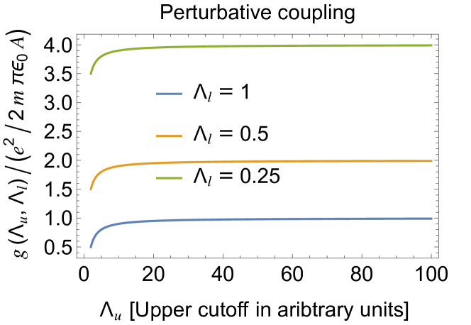
Figure 13: Normalized perturbative light-matter coupling $g(\Lambda_{u},\Lambda_{l})$ for different values of the lower cutoff $\Lambda_{l}$. The coupling constant increases rapidly and asymptotically reaches a fixed value which is inversely proportional to the lower cutoff $\Lambda_{l}$. For $\Lambda_{l}\to 0$ the perturbative coupling diverges.

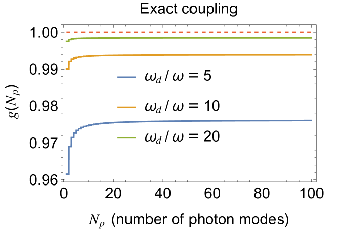
Figure 14: Non-perturbative multimode coupling $g(N_{p})$ as obtained from the exact solution for the free particle in Eq. (6) as a function of the number of photon modes $N_{p}$, for different values of the ratio $\omega_{d}/\omega$. The coupling constant increases rapidly and asymptotically reaches a plateau. The value of the plateau depends on the ratio $\omega_{d}/\omega$ but it never goes beyond unity.

Finally, it is important to mention that despite the fact that the free particle dispersion is always well defined and the coupling bounded, the observable mass $m_{e}=m/(1-g(N_{p}))$ as defined in Eq. (8) diverges when $g(N_{p})\rightarrow 1$. To tame the diverging $m_{e}$ in renormalization theory, the bare mass $m$ becomes cutoff-dependent and is promoted into $m(N_{p})$ such that to exactly cancel the diverging term $1/(1-g(N_{p}))$. For that purpose one takes $m(N_{p})=m_{e}(1-g(N_{p}))$ where $m_{e}$ is the measured physical electron mass. An important feature of our non-perturbative formula for the mass renormzalization is that the bare masses is always positive $m(N_{p})\geq 0$ because the total coupling $g(N_{p})\leq 1$ has an upper bound.

Appendix C Free Electron in the Length Gauge

In this appendix we provide the solution for single free particle coupled to one photon mode in the length gauge. Our purpose is to show that the renormalized dispersion of the electron in velocity and length gauges is the same. The Hamiltonian of one electron interacting with one photon mode in the length gauge is Rokaj et al. (2018)

$$\hat{H}_{\text{L}}=\frac{\hat{\textbf{p}}^{2}}{2m}+\frac{1}{2}\left[\hat{p}^{2}+\omega^{2}\left(\hat{q}\!-\!\frac{e\boldsymbol{\lambda}}{\omega}\cdot\hat{\textbf{r}}\right)^{2}\right],$$ (18)

We choose the polarization of the mode to be in the $x$ direction, $\boldsymbol{\lambda}=\lambda\mathbf{e}_{x}$, and in one spatial dimension we have

$$\hat{H}_{\text{L}}=-\frac{\hbar^{2}}{2m}\frac{\partial^{2}}{\partial x^{2}}-\frac{\hbar^{2}}{2}\frac{\partial^{2}}{\partial q^{2}}+\frac{\omega^{2}}{2}\left(q-\frac{\lambda}{\omega}x\right)^{2},$$ (19)

First we perform the scaling transformation $\bar{x}=e\lambda x/\omega$ and we introduce the parameter $\bar{m}=m\omega^{2}/\lambda^{2}$

$$\hat{H}_{L}=-\frac{\hbar^{2}}{2\bar{m}}\frac{\partial^{2}}{\partial\bar{x}^{2}}-\frac{\hbar^{2}}{2}\frac{\partial^{2}}{\partial q^{2}}+\frac{\omega^{2}}{2}\left(q-\bar{x}\right)^{2}.$$ (20)

The Hamiltonian can be solved by going into the mixed coordinates

$$w=\frac{\bar{m}\bar{x}+q}{\bar{m}+1}\;\;\textrm{and}\;\;u=q-\bar{x},$$ (21)

where it takes the simple form

$$\hat{H}_{\text{L}}=-\frac{\hbar^{2}}{2(\bar{m}+1)}\frac{\partial^{2}}{\partial w^{2}}-\frac{(\bar{m}+1)\hbar^{2}}{2\bar{m}}\frac{\partial^{2}}{\partial u^{2}}+\frac{\omega^{2}}{2}u^{2}.$$ (22)

In the above Hamiltonian we have a freely propagating polaritonic mode along the $w$ coordinate and harmonically confined mode along the $u$ coordinate. The $w$-dependent eigenfunctions are plane waves $f_{k_{w}}(w)=e^{\textrm{i}k_{w}w}$ while the eigenfunctions of the $u$ mode are Hermite functions $\Phi_{n}(u)$. Then, the energy spectrum of the system is

$$E_{k_{w},n}=\frac{\hbar^{2}k^{2}_{w}}{\bar{m}+1}+\hbar\widetilde{\omega}\left(n+\frac{1}{2}\right).$$ (23)

We note that the coordinates $w$ and $u$ are independent as they mutually commute $[\partial_{w},\partial_{u}]=[\partial_{w},u]=[\partial_{u},w]=0$. Comparing now the spectrum above of the free electron in the length gauge to the one derived in the velocity gauge given in Eq. (6) we see that they are not exactly the same. The length gauge spectrum $E_{k_{w},n}$ depends on the polaritonic quantum number $k_{w}$ while the spectrum in the velocity gauge on the quantum number $k_{x}$. Naturally, the question that arises is: How are $k_{x}$ and $k_{w}$ related?

To figure this out we will use the relation between the differential operators of $\partial_{x}$ and $\partial_{w}$. From the chain rule and neglecting the contribution of the photonic coordinate $q$ we have

$$\frac{\partial}{\partial w}=\frac{\partial\bar{x}}{\partial w}\frac{\partial x}{\partial\bar{x}}\ \frac{\partial}{\partial x}=\frac{\omega}{\lambda}\frac{\partial}{\partial x}\;\Longrightarrow\;k_{w}=\frac{\omega}{\lambda}k_{x}.$$ (24)

Substituting the relation above into Eq. (23) we find for the length gauge spectrum

$$E_{k_{x},n}=\frac{\hbar^{2}k^{2}_{x}}{2m}\left(1-\frac{\omega^{2}_{d}}{\widetilde{\omega}^{2}}\right)+\hbar\widetilde{\omega}\left(n+\frac{1}{2}\right).$$ (25)

The above result reproduces precisely the single-particle dispersion coupled to a single photon mode obtained in the velocity gauge in Ref. Rokaj et al. (2022b). This shows that the same free particle dispersion and the corresponding renormalized mass can be consistently obtained from both gauges.

We now revisit the issue of a mismatch between light and matter if both systems are not chosen consistently. To illustrate this, we keep a fixed length scale for the free particle as done in Sec. III and also keep the same sampling of 200 photon modes with cutoffs 0.01 and 0.5 au. We now sample a different discretized continuum with 200 photon modes but with cutoffs 0.001 and 0.05 au. Here, the upper cutoff is much lower than the energy of the first excitation of the free particle. For both continua, the coupling of the photon modes to the free particle is fixed to $\lambda=0.0019$. A comparison of the energy dispersion is shown in Fig. (15) where we find that the NRQED case with the upper cutoff (0.05 au) is off from the NRQED case with upper cutoff (0.5 au). The reason for this mismatch is that the photonic modes are all excited before the first electronic state can be populated making the matter degrees less important in the coupled system. This result shows that choosing length-scales consistently is very important in QED.

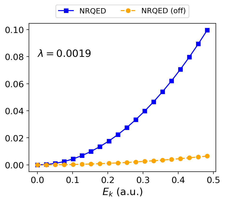
Figure 15: A comparison of the energy dispersion between two different sampling of the discretized photonic continuum. NRQED is the result presented in Fig. (1a) and NRQED (off) is the case where the upper cutoff is $0.05$ au.

Appendix D Model of a one-dimensional atom

The one-dimensional atomic system we consider features a single electron bound by a potential $V(x)$. The quantum mechanical Hamiltonian describing this system is given by

$$\hat{H}_{\text{atom}} =-\frac{\hbar^{2}}{2m_{e}}\frac{\partial^{2}}{\partial x^{2}}+V(x)\,.$$ (26)

Here we choose as binding potential in Eq. (26) a potential of the form

$$V(x) =-\frac{e^{2}}{4\pi\epsilon_{0}}\frac{v_{0}}{\cosh^{2}(k_{0}x)}\,,$$ (27)

where $v_{0}$ and $k_{0}$ are parameters that control the depth of the potential. For a single electron in the binding potential, the analytic spectrum of Eq. (26) is given as Landau and Lifshitz (1977)

$$E_{n} =-\frac{\hbar^{2}k_{0}^{2}}{8m_{e}}\left(\sqrt{1+\frac{8m_{e}v_{0}k_{e}}{\hbar^{2}k_{0}^{2}}}-(1+2n)\right)^{2},$$ (28)

where the quantum numbers are $n\in\mathbb{N}$ and $k_{e}=e^{2}/4\pi\epsilon_{0}$. The number of bound states can be controlled using $v_{0}$ and $k_{0}$. For our calculations we choose $v_{0}=10$ and $k_{0}=0.05$ which gives us 10 bound states of interest. We use the analytic results to benchmark our numerical implementation which agree perfectly.

Appendix E Model of a one-dimensional H₂ molecule

Our example of a molecular system considers the model for the H₂ molecule where the motion of all particles is restricted to one spatial dimension and the center-of-mass motion of the molecule can be separated off Lively et al. (2021); Albareda et al. (2021); Kreibich et al. (2001). The relevant coordinates of this model are the internuclear separation, $R$, and the electronic coordinates, $x_{1}$ and $x_{2}$. The Hamiltonian of the model system is given below

$$\hat{H}_{\text{mol}} =-\frac{1}{2\mu_{n}}\frac{\partial^{2}}{\partial R^{2}}+\frac{1}{R}+\frac{1}{\sqrt{(x_{1}-x_{2})^{2}+a_{\text{ee}}}}$$

$$\quad+\sum_{i=1}^{2}\left(-\frac{1}{2\mu_{\text{e}}}\frac{\partial^{2}}{\partial x_{i}^{2}}-\frac{1}{\sqrt{(x_{i}-R/2)^{2}+a_{\text{en}}}}\right.$$ (29)

$$\qquad\qquad\quad\left.-\frac{1}{\sqrt{(x_{i}+R/2)^{2}+a_{\text{en}}}}\right),$$

where $\mu_{\text{e}}=2M_{n}/(2M_{n}+1)$ and $\mu_{n}=M_{n}/2$ are the reduced observable electronic and nuclei masses, respectively. We take the proton mass to be $M_{n}=1836\,m_{e}$. The electron-electron and electron-nuclear interaction terms are represented by soft-Coulomb potentials where the soft-Coulomb parameters take values $a_{\text{ee}}\!=\!2$ and $a_{\text{en}}\!=\!1$. For the model, the PESs are defined by the following electronic eigenvalue problem: $\hat{H}_{\text{el}}(x_{1},x_{2};R)\Phi_{k}(x_{1},x_{2};R)=E_{k}(R)\Phi_{k}(x_{1},x_{2};R)$ where $\hat{H}_{\text{el}}=\hat{H}_{\text{H}_{2}}-\hat{T}_{n}$ where $\hat{T}_{n}=-\frac{1}{2\mu_{n}}\frac{\partial^{2}}{\partial R^{2}}$. We show the first five numerically exact PESs in Fig. (16) for the case where we do not couple to the photonic continuum (i.e. for $N_{p}=0$). The mean nuclear equilibrium position is $R_{\text{eq}}=1.9$ a.u. with the corresponding ground-state energy $E_{0}=-1.4843$ a.u. Applying the harmonic approximation to the ground-state PES as in App. F we obtain the harmonic frequency $\omega_{e}=0.020455$ a.u. of the nuclear degrees.

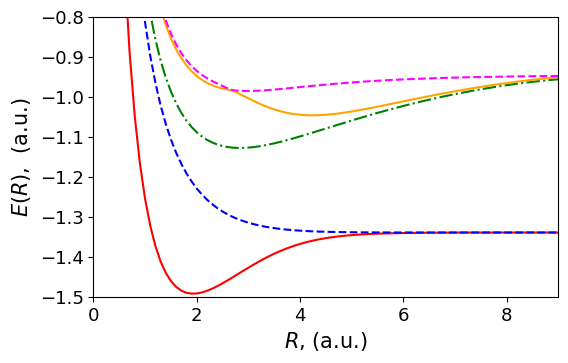
Figure 16: The first five numerically exact PESs of the 1D hydrogen molecule H₂ for $N_{p}=0$. The harmonic approximation to the ground-state PES has the harmonic frequency $\omega_{e}=0.020455$ a.u. for the nuclear degrees.

We note that when we couple the molecule to the discretized continuum, we used the bare proton mass $M=1836\,m$ where the bare electronic mass is $m=1$. At the equilibrium position, we compute the ground-state density for NRQED and QM for the case when the renormalized mass is obtained with the lowest 50 of the 200 sampled photon modes. In Fig. (17), we show the ground-state density where the QM case is more bound when compared to the NRQED. The reason for this is discussed in Sec. IV.1 of the main text.

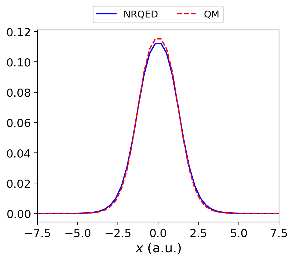
Figure 17: A comparison of the ground-state density of the H₂ molecule at the equilibrium position $R_{\text{eq}}=1.9$ a.u. between NRQED and QM for the case of $N_{p}=50$ photon modes.

Appendix F Morse and harmonic approximation to the H₂ PES

In this section we provide details of the Morse and harmonic approximation to the numerical exact ground-state H₂ PoPES of the NRQED and QM settings. To do this, we first consider the Morse potential

$$V_{\text{M},i}(R)=D_{e,i}\left(e^{-a_{i}(R-R_{\text{eq}})}-1\right)^{2}+C_{i}\,,$$ (30)

where the parameter “$a$” controls the ‘width’ of the potential (i.e., the smaller “$a$” is, the larger the well), $C$ is a constant shift in the PES and $i=\{\textrm{NRQED},\textrm{QM}\}$. Since we have access to all the parameters of Eq. (30) except for the $a$ parameter, this makes the fitting procedure easier. To fit the Morse potential to the exact results of NRQED and QM settings, we employ the “curve_fit” function of scipy and the corresponding $a$ parameter values of NRQED and QM are given in Tab. (2). The results of the fit are plotted in Fig. (18).

Level of theory	Morse parameter $a$	Harmonic frequency $\omega_{e}$
QM	$1.1306567$	$0.0202009$
NRQED	$1.18811731$	$0.0217312$

Table 2: The values of the $a$ parameter of the Morse potential resulting from the fit and the deduced harmonic frequency $\omega_{e}$ for the case of $N_{p}=50$ photon modes. The units are in (a.u.).

Since we are interested in the influence the continuum has on the nuclear degrees, we connect the $a$ parameter to the nuclei mass by employing the harmonic potential fit to the Morse potential around the equilibrium $R_{\text{eq}}$. The harmonic potential is given by

$$V_{\text{H},i}(R)=\frac{1}{2}k_{i}\left(R-R_{\text{eq}}\right)^{2}+C_{i}\,,$$ (31)

where $k$ is the force constant of the bond which is related to the reduced nuclei mass as $k=\mu_{n}\,\omega_{e}^{2}$ and $\omega_{e}$ is the vibrational frequency of the potential. From the above considerations, we have the relation $k=2D_{e}a^{2}$ from which we have $\omega_{e}=\sqrt{2D_{e}a^{2}/\mu_{n}}$.

To obtain the approximate vibrational harmonic frequency of the NRQED setting, we used the bare proton mass $M=1836\,m$ where the bare electronic mass is $m=1$. The renormalized proton mass is deduced from the energy dispersion for free interacting protons coupled to the electromagnetic continuum. The energy dispersion is similar to Eq. (6) where the diamagnetic frequency has a dependence on the nuclear charge.

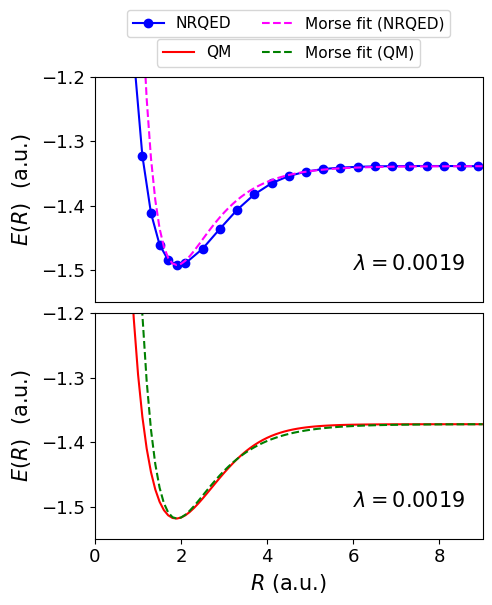
Figure 18: Morse potential fit to the numerical exact ground-state PES of the H₂ molecule for NRQED and QM for the case of $N_{p}=50$ photon modes.

References

- Ruggenthaler et al. (2018) Michael Ruggenthaler, Nicolas Tancogne-Dejean, Johannes Flick, Heiko Appel, and Angel Rubio, “From a quantum-electrodynamical light–matter description to novel spectroscopies,” Nature Reviews Chemistry 2, 0118 (2018).
- Flick et al. (2018) Johannes Flick, Nicholas Rivera, and Prineha Narang, “Strong light-matter coupling in quantum chemistry and quantum photonics,” Nanophotonics 7, 1479–1501 (2018).
- Ruggenthaler et al. (2023) Michael Ruggenthaler, Dominik Sidler, and Angel Rubio, “Understanding polaritonic chemistry from ab initio quantum electrodynamics,” Chem. Rev. (2023), 10.1021/acs.chemrev.2c00788.
- Schlawin et al. (2022) Frank Schlawin, D. M. Kennes, and Michael A. Sentef, “Cavity quantum materials,” Appl. Phys. Rev. 9, 011312 (2022).
- Ebbesen (2016) Thomas W. Ebbesen, “Hybrid light–matter states in a molecular and material science perspective,” Accounts of Chemical Research 49, 2403–2412 (2016).
- Garcia-Vidal et al. (2021) Francisco J. Garcia-Vidal, Cristiano Ciuti, and Thomas W. Ebbesen, “Manipulating matter by strong coupling to vacuum fields,” Science 373, 178 (2021).
- Kéna-Cohen and Forrest (2010) S. Kéna-Cohen and S. R. Forrest, “Room-temperature polariton lasing in an organic single-crystal microcavity,” Nat. Photonics 4, 371–375 (2010).
- Hutchison et al. (2012) James A. Hutchison, Tal Schwartz, Cyriaque Genet, Eloïse Devaux, and Thomas W. Ebbesen, “Modifying chemical landscapes by coupling to vacuum fields,” Angewandte Chemie International Edition 51, 1592–1596 (2012).
- Galego et al. (2016) Javier Galego, Francisco J. Garcia-Vidal, and Johannes Feist, “Suppressing photochemical reactions with quantized light fields,” Nature Communications 7, 13841 (2016).
- Coles et al. (2014) David M. Coles, Yanshen Yang, Yaya Wang, Richard T. Grant, Robert A. Taylor, Semion K. Saikin, Alán Aspuru-Guzik, David G. Lidzey, Joseph Kuo-Hsiang Tang, and Jason M. Smith, “Strong coupling between chlorosomes of photosynthetic bacteria and a confined optical cavity mode,” Nature Communications 5, 5561 (2014).
- Schäfer et al. (2019) Christian Schäfer, Michael Ruggenthaler, Heiko Appel, and Angel Rubio, “Modification of excitation and charge transfer in cavity quantum-electrodynamical chemistry,” PNAS 116, 4883–4892 (2019).
- Zhong et al. (2016) Xiaolan Zhong, Thibault Chervy, Shaojun Wang, Jino George, Anoop Thomas, James A. Hutchison, Eloise Devaux, Cyriaque Genet, and Thomas W. Ebbesen, “Non-radiative energy transfer mediated by hybrid light-matter states,” Angewandte Chemie International Edition 55, 6202–6206 (2016).
- Chervy et al. (2016) Thibault Chervy, Jialiang Xu, Yulong Duan, Chunliang Wang, Loïc Mager, Maurice Frerejean, Joris A. W. Münninghoff, Paul Tinnemans, James A. Hutchison, Cyriaque Genet, Alan E. Rowan, Theo Rasing, and Thomas W. Ebbesen, “High-efficiency second-harmonic generation from hybrid light-matter states,” Nano Lett. 16, 7352–7356 (2016).
- Barachati et al. (2018) Fábio Barachati, Janos Simon, Yulia A. Getmanenko, Stephen Barlow, Seth R. Marder, and Stéphane Kéna-Cohen, “Tunable third-harmonic generation from polaritons in theultrastrong coupling regime,” ACS Photonics 5, 119–125 (2018).
- Welakuh and Narang (2023) Davis M. Welakuh and Prineha Narang, “Tunable and efficient harmonic generation from strongly coupled light-matter system,” ACS Photonics 10, 383–393 (2023).
- Welakuh and Narang (2022a) Davis M. Welakuh and Prineha Narang, “Nonlinear optical processes in centrosymmetric systems by strong- coupling-induced symmetry breaking,” arXiv:2203.00691 (2022a), 10.48550/arXiv.2202.11117.
- Thompson et al. (2006) James K. Thompson, Jonathan Simon, Huanqian Loh, and Vladan Vuletić, “A high-brightness source of narrowband, identical-photon pairs,” Science 313, 74–77 (2006).
- Schäfer et al. (2022) Christian Schäfer, Johannes Flick, Enrico Ronca, Prineha Narang, and Angel Rubio, “Shining light on the microscopic resonant mechanism responsible for cavity-mediated chemical reactivity,” Nat Commun 13, 7817 (2022).
- Thomas et al. (2019) A. Thomas, L. Lethuillier-Karl, K. Nagarajan, R. M. A. Vergauwe, J. George, T. Chervy, A. Shalabney, E. Devaux, C. Genet, J. Moran, and T. W. Ebbesen, “Tilting a ground-state reactivity landscape by vibrational strong coupling,” Science 363, 615–619 (2019).
- Peter et al. (2005) E. Peter, P. Senellart, D. Martrou, A. Lemaître, J. Hours, J. M. Gérard, and J. Bloch, “Exciton-photon strong-coupling regime for a single quantum dot embedded in a microcavity,” Phys. Rev. Lett. 95, 067401 (2005).
- Latini et al. (2021) Simone Latini, Dongbin Shin, Shunsuke A. Sato, Christian Schäfer, Umberto De Giovannini, Hannes Hübener, and Angel Rubio, “The ferroelectric photo ground state of srtio¡sub¿3¡/sub¿: Cavity materials engineering,” Proceedings of the National Academy of Sciences 118, e2105618118 (2021).
- Liu et al. (2015) Xiaoze Liu, Tal Galfsky, Zheng Sun, Fengnian Xia, Erh chen Lin, Yi-Hsien Lee, Stéphane Kéna-Cohen, and Vinod M. Menon, “Strong light–matter coupling in two-dimensional atomic crystals,” Nature Photonics 9, 1749–4893 (2015).
- Appugliese et al. (2022) F. Appugliese, J. Enkner, G. L. Paravicini-Bagliani, M. Beck, C. Reichl, W. Wegscheider, G. Scalari, C. Ciuti, and J. Faist, “Breakdown of topological protection by cavity vacuum fields in the integer quantum Hall effect,” Science 375, 1030–1034 (2022).
- Paravicini-Bagliani et al. (2019) G. L. Paravicini-Bagliani, F. Appugliese, E. Richter, S. Fallahi, F. Valmorra, J. Keller, M. Beck, N. Bartolo, C. Rössler, T. Ihn, K. Ensslin, C. Ciuti, G. Scalari, and J. Faist, “Magneto-transport controlled by Landau polariton states,” Nat. Phys. 15, 186–190 (2019).
- Rokaj et al. (2022a) Vasil Rokaj, Markus Penz, Michael A. Sentef, Michael Ruggenthaler, and Angel Rubio, “Polaritonic hofstadter butterfly and cavity control of the quantized hall conductance,” Phys. Rev. B 105, 205424 (2022a).
- Rokaj et al. (2023a) Vasil Rokaj, Jie Wang, John Sous, Markus Penz, Michael Ruggenthaler, and Angel Rubio, “On the topological protection of the quantum hall effect in a cavity,” (2023a), arXiv:2305.10558 [cond-mat.mes-hall] .
- Chikkaraddy et al. (2016) Rohit Chikkaraddy, Bart de Nijs, Felix Benz, Steven J. Barrow, Oren A. Scherman, Edina Rosta, Angela Demetriadou, Peter Fox, Ortwin Hess, and Jeremy J. Baumberg, “Single-molecule strong coupling at room temperature in plasmonic nanocavities,” Nature 535, 127–130 (2016).
- Ojambati et al. (2019) Oluwafemi S. Ojambati, Rohit Chikkaraddy, William D. Deacon, Matthew Horton, Dean Kos, Vladimir A. Turek, Ulrich F. Keyser, and Jeremy J. Baumberg, “Quantum electrodynamics at room temperature coupling a single vibrating molecule with a plasmonic nanocavity,” Nat Commun 10, 1049 (2019).
- Dicke (1954) R. H. Dicke, “Coherence in spontaneous radiation processes,” Phys. Rev. 93, 99 (1954).
- Tavis and Cummings (1968) Michael Tavis and Frederick W. Cummings, “Exact solution for an n-molecule–radiation-field hamiltonian,” Phys. Rev. 170, 379–384 (1968).
- Ruggenthaler et al. (2014) Michael Ruggenthaler, Johannes Flick, Camilla Pellegrini, Heiko Appel, Ilya V. Tokatly, and Angel Rubio, “Quantum-electrodynamical density-functional theory: Bridging quantum optics and electronic-structure theory,” Phys. Rev. A 90, 012508 (2014).
- Flick et al. (2015) Johannes Flick, Michael Ruggenthaler, Heiko Appel, and Angel Rubio, “Kohn-sham approach to quantum electrodynamical density-functional theory: Exact time-dependent effective potentials in real space,” Proc. Natl. Acad. Sci. U. S. A. 112, 15285–15290 (2015).
- Haugland et al. (2020) Tor S. Haugland, Enrico Ronca, Eirik F. Kjonstad, Angel Rubio, and Henrik Koch, “Coupled cluster theory for molecular polaritons: Changing ground and excited states,” Phys. Rev. X 10, 041043 (2020).
- Riso et al. (2022) Rosario R. Riso, Tor S. Haugland, Enrico Ronca, and Henrik Koch, “Molecular orbital theory in cavity qed environments,” Nat Commun 13, 1368 (2022).
- Galego et al. (2017) Javier Galego, Francisco J. Garcia-Vidal, and Johannes Feist, “Many-molecule reaction triggered by a single photon in polaritonic chemistry,” Phys. Rev. Lett. 119, 136001 (2017).
- Gonzalez-Ballestero et al. (2016) Carlos Gonzalez-Ballestero, Johannes Feist, Eduardo Gonzalo Badía, Esteban Moreno, and Francisco J. Garcia-Vidal, “Uncoupled dark states can inherit polaritonic properties,” Phys. Rev. Lett. 117, 156402 (2016).
- Purcell (1995) E. M. Purcell, “Spontaneous emission probabilities at radio frequencies,” in Confined Electrons and Photons: New Physics and pplications (Springer US, Boston, MA, 1995) pp. 839–839.
- Casimir and Polder (1948) H. B. G. Casimir and D. Polder, “The influence of retardation on the london-van der waals forces,” Phys. Rev. 73, 360–372 (1948).
- Bethe and Salpeter (1957) Hans A. Bethe and Edwin E. Salpeter, Quantum Mechanics of One- and Two-Electron Atoms (Springer-Verlag Berlin, Heidelberg, 1957).
- Weisskopf and Wigner (1930) V. Weisskopf and E. Wigner, “Berechnung der natürlichen linienbreite auf grund der diracschen lichttheorie,” Zeitschrift für Physik 63, 54–73 (1930).
- Bužek et al. (1999) V. Bužek, G. Drobný, Min Gyu Kim, M. Havukainen, and P. L. Knight, “Numerical simulations of atomic decay in cavities and material media,” Phys. Rev. A 60, 582–592 (1999).
- Flick et al. (2017) Johannes Flick, Michael Ruggenthaler, Heiko Appel, and Angel Rubio, “Atoms and molecules in cavities, from weak to strong coupling in quantum-electrodynamics (qed) chemistry,” Proceedings of the National Academy of Sciences 114, 3026–3034 (2017).
- Spohn (2004) Herbert Spohn, Dynamics of charged particles and their radiation field (Cambridge university press, 2004).
- Cohen‐Tannoudji et al. (1989) Claude Cohen‐Tannoudji, Jacques Dupont‐Roc, and Gilbert Grynberg, Photons and Atoms: Introduction to Quantum Electrodynamics (John Wiley & Sons, Inc., 1989).
- Hainzl and Seiringer (2002) Christian Hainzl and Robert Seiringer, “Mass renormalization and energy level shift in non-relativistic qed,” Adv. Theor. Math. Phys 6, 847–871 (2002).
- Landau and Lifshitz (1977) I. D. Landau and E. M. Lifshitz, Quantum Mechanics Non-Relativistic Theory, 3rd ed. (Pergamon Press, Oxford, 1977).
- Albareda et al. (2021) Guillermo Albareda, Kevin Lively, Shunsuke A. Sato, Aaron Kelly, and Angel Rubio, “Conditional wave function theory: A unified treatment of molecular structure and nonadiabatic dynamics,” Journal of Chemical Theory and Computation 17, 7321–7340 (2021).
- Mandl and Shaw (2010) Franz Mandl and Graham Shaw, Quantum Field Theory (Wiley, 2010).
- Rokaj et al. (2018) Vasil Rokaj, Davis M Welakuh, Michael Ruggenthaler, and Angel Rubio, “Light–matter interaction in the long-wavelength limit: no ground-state without dipole self-energy,” Journal of Physics B: Atomic, Molecular and Optical Physics 51, 034005 (2018).
- Schäfer et al. (2020) Christian Schäfer, Michael Ruggenthaler, Vasil Rokaj, and Angel Rubio, “Relevance of the quadratic diamagnetic and self-polarization terms in cavity quantum electrodynamics,” ACS Photonics 7, 975–990 (2020).
- Craig and Thirunamachandran (1998) D.P. Craig and T. Thirunamachandran, Molecular Quantum Electrodynamics: An Introduction to Radiation-molecule Interactions, Dover Books on Chemistry Series (Dover Publications, 1998).
- Rokaj et al. (2022b) Vasil Rokaj, Michael Ruggenthaler, Florian G. Eich, and Angel Rubio, “The free electron gas in cavity quantum electrodynamics,” Phys. Rev. Research 4, 013012 (2022b).
- Chen (2008) Thomas Chen, “Infrared renormalization in nonrelativistic qed and scaling criticality,” J. Funct. Anal. 254, 2555–2647 (2008).
- Fröhlich and Pizzo (2010) Jürg Fröhlich and Alessandro Pizzo, “Renormalized electron mass in nonrelativistic qed,” Commun. Math. Phys. 294, 439–470 (2010).
- Van Hove (1952) Leon Van Hove, “Les difficultés de divergences pour un modèle particulier de champ quantifié,” Physica 18, 145–159 (1952).
- Han and Madsen (2010) Yong-Chang Han and Lars Bojer Madsen, “Comparison between length and velocity gauges in quantum simulations of high-order harmonic generation,” Phys. Rev. A 81, 063430 (2010).
- Bandrauk et al. (2013) A. D. Bandrauk, F. Fillion-Gourdeau, and E. Lorin, “Atoms and molecules in intense laser fields: gauge invariance of theory and models,” J. Phys. B: At. Mol. Opt. Phys. 46, 153001 (2013), 10.1088/0953-4075/46/15/153001.
- Rokaj et al. (2023b) Vasil Rokaj, Simeon I. Mistakidis, and H. R. Sadeghpour, “Cavity induced collective behavior in the polaritonic ground state,” SciPost Phys. 14, 167 (2023b).
- Flick et al. (2019) Johannes Flick, Davis M. Welakuh, Michael Ruggenthaler, Heiko Appel, and Angel Rubio, “Light-matter response in nonrelativistic quantum electrodynamics,” ACS Photonics 6, 2757–2778 (2019).
- Welakuh et al. (2022) Davis M. Welakuh, Johannes Flick, Michael Ruggenthaler, Heiko Appel, and Angel Rubio, “Frequency-dependent sternheimer linear-response formalism for strongly coupled light-matter systems,” J. Chem. Theory Comput. 18, 4354–4365 (2022).
- Welakuh and Narang (2022b) Davis M. Welakuh and Prineha Narang, “Transition from lorentz to fano spectral line shapes in non-relativistic quantum electrodynamics,” ACS Photonics 9, 2946–2955 (2022b).
- Feist and Garcia-Vidal (2015) Johannes Feist and Francisco J. Garcia-Vidal, “Extraordinary exciton conductance induced by strong coupling,” Phys. Rev. Lett. 114, 196402 (2015).
- Flick and Narang (2018) Johannes Flick and Prineha Narang, “Cavity-correlated electron-nuclear dynamics from first principles,” Phys. Rev. Lett. 121, 113002 (2018).
- Hiroshima and Spohn (2005) Fumio Hiroshima and Herbert Spohn, “Mass renormalization in nonrelativistic quantum electrodynamics,” Journal of Mathematical Physics 46, 042302 (2005).
- Loudon (2000) Rodney Loudon, The Quantum Theory of Light (Oxford University Press, 2000).
- Lively et al. (2021) Kevin Lively, Guillermo Albareda, Shunsuke A. Sato, Aaron Kelly, and Angel Rubio, “Simulating vibronic spectra without born–oppenheimer surfaces,” J. Phys. Chem. Lett. 12, 3074–3081 (2021).
- Kreibich et al. (2001) Thomas Kreibich, Manfred Lein, Volker Engel, and E. K. U. Gross, “Even-harmonic generation due to beyond-born-oppenheimer dynamics,” Phys. Rev. Lett. 87, 103901 (2001).