Probing the early Milky Way with GHOST spectra of an extremely metal-poor star in the Galactic disk

Abstract

Pristine_183.6849+04.8619 (P1836849) is an extremely metal-poor ([Fe/H]$=-3.3\pm 0.1$) star on a prograde orbit confined to the Galactic disk. Such stars are rare and may have their origins in protogalactic fragments that formed the early Milky Way, in low mass satellites accreted later, or forming in situ in the Galactic plane. Here we present a chemo-dynamical analysis of the spectral features between $3700-11000$ Å from a high-resolution spectrum taken during Science Verification of the new Gemini High-resolution Optical SpecTrograph (GHOST). Spectral features for many chemical elements are analysed (Mg, Al, Si, Ca, Sc, Ti, Cr, Mn, Fe, Ni), and valuable upper limits are determined for others (C, Na, Sr, Ba). This main sequence star exhibits several rare chemical signatures, including (i) extremely low metallicity for a star in the Galactic disk, (ii) very low abundances of the light $\alpha$-elements (Na, Mg, Si) compared to other metal-poor stars, and (iii) unusually large abundances of Cr and Mn, where [Cr, Mn/Fe]${}_{\rm NLTE}>+0.5$. A comparison to theoretical yields from supernova models suggests that two low mass Population III objects (one 10 M_⊙ supernova and one 17 M_⊙ hypernova) can reproduce the abundance pattern well (reduced $\chi^{2}<1$). When this star is compared to other extremely metal-poor stars on quasi-circular, prograde planar orbits, differences in both chemistry and kinematics imply there is little evidence for a common origin. The unique chemistry of P1836849 is discussed in terms of the earliest stages in the formation of the Milky Way.

1 Introduction

Low-metallicity stars are among the oldest stars in the Galaxy. Cosmological simulations suggest that these pristine stars formed within 2–3 Gyr after the Big Bang, preferentially in low-mass protogalactic systems (e.g.,  Starkenburg et al., 2017b; El-Badry et al., 2018; Sestito et al., 2021). As the Milky Way (MW) grows, these protogalactic systems contribute their stars, gas, and dark matter contents throughout the proto-MW, including some into planar orbits that will later form the disk (Sestito et al., 2021; Santistevan et al., 2021). Low-mass systems accreted later are expected to disperse their stars primarily into the halo (Bullock & Johnston, 2005; Johnston et al., 2008), though simulations show that they can also contribute stars with nearly circular orbits on the Galactic disk (Abadi et al., 2003; Scannapieco et al., 2011; Sestito et al., 2021; Santistevan et al., 2021). Contributions to the disk are also possible from an in-situ component of stars formed from the deposited gas (Abadi et al., 2003; Navarro et al., 2018; Yu et al., 2021), and even the chaotic pre-disk epochs when stars are born in irregular configurations (e.g.,  Belokurov & Kravtsov, 2022, 2023). Some simulations suggest the transition from "bursty" to "steady" star formation occurs after a stable hot gaseous halo surrounds the MW progenitor, impacting the gas accretion mechanisms, such that a coherent disk forms via dissipative accretion, i.e., when the angular momentum of the accreting gas is aligned with the forming galaxy disk (e.g., Sales et al., 2012; Stern et al., 2021; Hafen et al., 2022). This later formation means that "steady" star formation in the disk would occur from pre-enriched gas.

Nevertheless, some extremely metal-poor (EMP, [Fe/H]$<-3$) stars have been found confined to the Galactic plane (e.g.,  Sestito et al., 2019, 2020; Venn et al., 2020; Kielty et al., 2021; Fernández-Alvar et al., 2021; Cordoni et al., 2021). It is not clear if these stars occupy the extreme metal-poor extension of the thin disk or the high rotating tail of hotter MW structures like the thick disk or the halo. A comparison of EMP stars with planar orbits on prograde vs retrograde orbits does show a net preference for prograde stars in both observations (Sestito et al., 2020) and simulations (Sestito et al., 2021; Santistevan et al., 2021). If true, it could suggest an additional source of prograde EMP stars compared to retrograde stars, which are almost certainly accreted from protogalactic fragments and low mass satellites during the early Galactic assembly. For example, it is possible that some quasi-circular prograde planar EMP stars may have formed in situ at very early times in the formation of the Galactic proto-disk. Alternatively, a dwarf galaxy whose orbit was brought into the disk and circularized before being tidally disrupted could have added its stars to the proto-Galactic disk.

While dynamics alone might not help us to clearly identify planar stars that formed in situ, chemo-dynamical analyses can provide more clues. The most chemically pristine stars in the Milky Way are expected to have been enriched by only one or a few Population III (Pop III) supernovae or hypernovae events (e.g.,  Frebel, Kirby & Simon, 2010; Heger et al., 2012; Ishigaki et al., 2018). Recently, the aluminum abundance in metal-poor stars has been proposed as a way to disentangle stars that formed in situ from those accreted from satellites (e.g.,  Das, Hawkins & Jofré, 2020; Belokurov & Kravtsov, 2022). However this indicator is limited to stars with [Fe/H]$>-2$. At lower metallicities, differences in the [Al/Fe] (and most other light element ratios) are less distinct between different stellar populations (e.g., Yong et al., 2013, 2021; Aoki et al., 2013; Skúladóttir et al., 2021). Below [Fe/H]=$-3$, it has been suggested that neutron-capture elements may differ between EMP stars in ultra-faint dwarf (UFD) galaxies when compared with similar stars in the Galactic halo and classical dwarf galaxies (e.g., Jablonka et al., 2015; Ji et al., 2019; Sitnova et al., 2021), particularly the [Sr/Ba] ratios. If EMP stars have been enriched by a very small number of supernovae, then the ultimate goal would be to use this information to trace their origins back to their host. This is work in progress, as nucleosynthetic yields and our understanding of galaxy formation and early star formation improve.

Currently, only seven EMP stars with quasi-circular prograde planar orbits have had their detailed chemical abundances analysed; SDSS J102915$+$172927 (Caffau et al., 2011, 2012), 2MASS J1808202$-$5104378 (Schlaufman et al., 2018; Mardini et al., 2022a), four stars from the SkyMapper survey (when orbits from Cordoni et al. 2021 are cross matching with abundances from Yong et al. 2021), and Pristine_183.6849+04.8619 (P1836849, Venn et al. 2020). P1836849 was discovered as part of the spectroscopic follow-up studies to the Pristine survey (Starkenburg et al., 2017a), a narrow-band imaging survey using MegaCam at the Canada-France-Hawaii Telescope. Using a specialized Ca ii HK filter in combination with broad-band photometry, the Pristine survey has demonstrated high efficiency in the detection of metal-poor stars (i.e., $>$56 percent accuracy at ${\rm[Fe/H]}\leq-2.5$, Youakim et al., 2017; Aguado et al., 2019; Martin et al., 2023). P1836849 was noted as an EMP with a quasi-circular prograde orbit (Venn et al., 2020), which, as discussed above, is uncommon amongst EMP stars.

In this paper, we present a new orbital and chemical analysis of P1836849. New spectra were taken during the System Verification observations of the new Gemini High-resolution Optical SpecTrograph (GHOST, Pazder et al., 2020) at Gemini South as described in Section 2. GHOST is the ideal instrument as it has very high efficiency and wide spectral coverage (3700 - 11000 Å), making it possible to estimate precise abundances for a large number of elements. The potential of GHOST spectroscopy has been made clear by the analysis of two stars in the Reticulum II dwarf galaxy (Hayes et al., 2023) and one metal-poor star in the Milky Way that was either accreted from a low mass satellite or formed in one of the low-mass building blocks of the proto-Galaxy (Sestito et al., 2023a). The determination of new orbital and stellar parameters are described in Section 3. Our spectral line analyses and chemical abundance determinations from model atmospheres are described in Sections 4 and 5. A comparison to other prograde EMP stars in the disk, EMP stars in the MW halo and nearby low-mass galaxies, and theoretical nucleosynthetic yields are presented in Section 6, as the basis for our discussion on the origins of this star. Overall, we note that the higher efficiency and larger wavelength coverage of GHOST makes this an excellent instrument for the determination of precision chemical abundances and radial velocities for stars in the Local Group (i.e., G$\lesssim$19, dependent on the signal-to-noise requirements).

Table 1: The long and short names of the EMP quasi-circular planar stars, and their Gaia DR3 source IDs and photometric indices (G and BP$-$RP). Reddening (A_V) for the first three stars is from Schlafly & Finkbeiner (2011) and used to calculate our heliocentric distances (see text). ^∗Reddening and distances for the last four stars are taken from Cordoni et al. (2021).

Target	Short name	source ID	G	BP$-$RP	AV	D
			(mag)	(mag)	(mag)	(kpc)
Pristine_183.6849+04.8619	P1836849	3894267325687326592	14.82	0.62	0.05	$1.20\pm 0.12$
SDSS J102915+172927	SDSS J102915	3890626773968983296	16.53	0.79	0.07	$1.49\pm 0.32$
2MASS J18082002-5104378	2MASS J18082002	6702907209758894848	11.75	0.91	0.31	$0.59\pm 0.01$
SMSS J133308.90-465407.9	SMSS J133308	6083921475163462528	12.22	1.28	0.10	$3.83\pm 0.96^{*}$
SMSS J190556.70-454724.2	SMSS J190556	6710975288644549760	12.90	1.22	0.07	$6.19\pm 1.54^{*}$
SMSS J190836.24-401623.5	SMSS J190836	6717349947823371776	13.10	1.27	0.10	$5.62\pm 0.66^{*}$
SMSS J232121.57-160505.4	SMSS J232121	2406023396270909440	12.53	0.95	0.02	$1.10\pm 0.20^{*}$

2 Data

2.1 Target Selection

During early testing and calibration of the Pristine survey, spectroscopic observations of bright (V$<15$) metal-poor candidates were observed with the Canada-France-Hawaii Telescope’s ESPaDoNS high resolution spectrograph (Donati et al., 2006). Out of 115 metal-poor candidates analysed by Venn et al. (2020), one target, Pristine_183.6849+04.861 (P1836849), was found to have an unusual chemical and kinematic behaviour. Orbital analysis using Gaia DR2 (Gaia Collaboration et al., 2016, 2018) showed that P1836849 has a quasi-circular orbit (eccentricity $\epsilon\sim 0.3$) with a relatively small maximum height from the MW plane (Z_max = 1.2 kpc). The object is close to the Sun (distance $\sim 1.05$ kpc) and to its apocentre (R${}_{\rm apo}=8.4$ kpc; see Table 3). Despite its low metallicity ([Fe/H]$=-3.25$; see Section 4), this star was unlikely to be a MW halo interloper because of its low Mg and low Na abundances ([Mg/Fe] $=0.13$, [Na/Fe] $=-0.18$; although these were NLTE corrected abundances, and consistent with the NLTE corrected abundances of other EMP MW halo stars examined by Venn et al. 2020). At the time, it was proposed as an accreted object early in the Galaxy’s lifetime. Here, we update the analysis of P1836849, starting with its basic information from Gaia DR3 (Gaia Collaboration et al., 2023) provided in Table 1.

Table 2: GHOST science and calibration exposures for P1836849 (Program ID: GS-2023A-SV-101). These observations were taken in the standard resolution, single object mode, with 2x2 binning.

Filetype	Arm	texp	Nexp	SNR @$\lambda$
		(s)		(Å)
Science
GS-2023A-SV-101-19-001	Blue	1800	x2	60 @4130
	Red	1200	x3	90 @6500
Calibrations
GS-CAL20230511-15-001	arc	720	–	–
GS-CAL20230511-14-001	flat	30	–	–
GS-CAL20230511-20-001	2x2 bias	–	–	–
GS-CAL20230510-1-001	1x1 bias	–	–	–

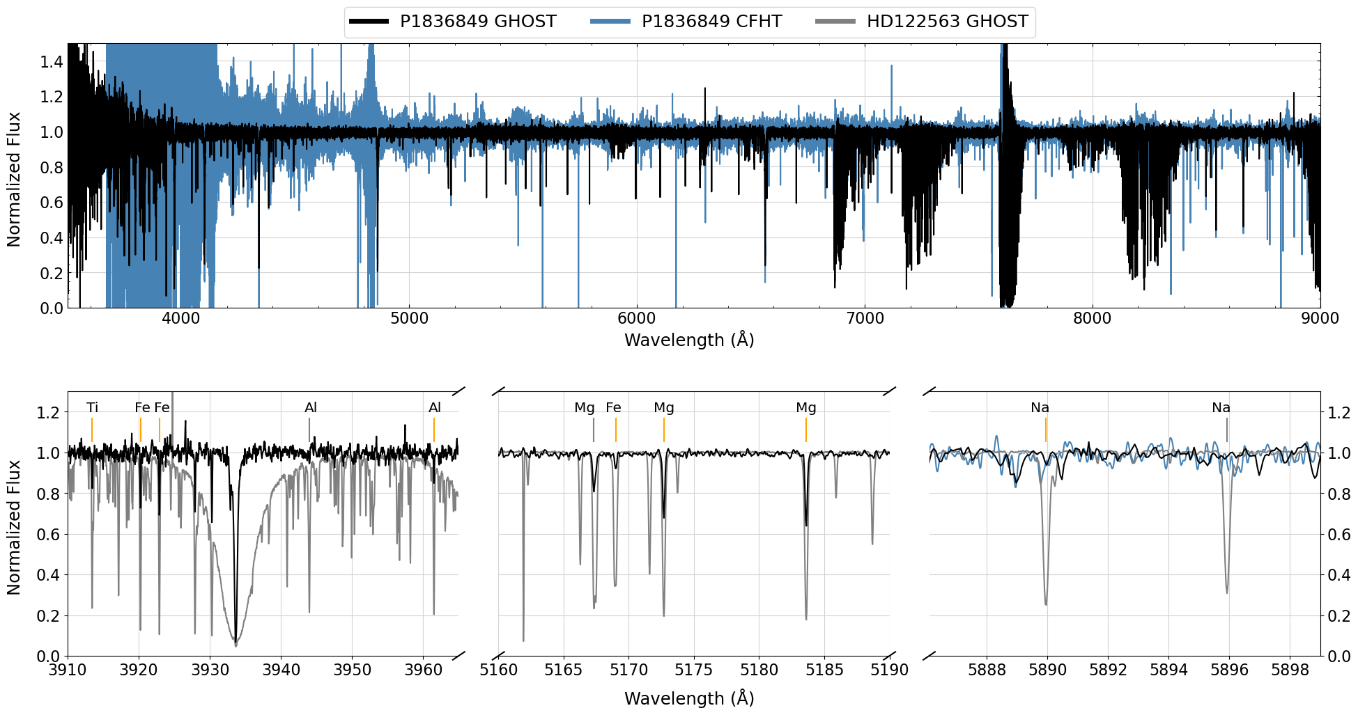
Figure 1: Top panel: Spectrum of P1836849 from Gemini-GHOST (black, [Fe/H]$=-3.3$) is compared to the CFHT-ESPaDoNS observation (blue), over a wide spectral region from $3500-9000$ Å. Lower panel: Three spectral windows show Ti ii, Fe i, and Al i lines from $3910-3965$ Å, the Mg i and Fe i lines from $5150-5200$ Å, and the absence of the Na d lines in P1836849 from $5885-5900$ Å. A GHOST spectrum for HD 122563 (grey, note [Fe/H]$=-2.8$) is shown for comparison in the lower panels. We also show the CFHT spectrum for P1836849 near the Na d lines only to emphasize the weakness of these features. Spectral lines used in our chemical analysis are as marked in orange.

2.2 GHOST observations

P1836849 was observed on 10 May 2023, during the System Verification run of the new GHOST spectrograph (Ireland et al., 2012; McConnachie et al., 2022). The instrument setup chosen was the standard resolution mode (SR: $R\sim 50,000$) and target mode IFU1:Target—IFU2:Sky. Each IFU in this SR mode includes 7 hexagonal fibers in a compact arrangement projected to 1.2 arcseconds on-sky. These fibres are then aligned to form a pseudo-slit which enters the spectrograph, delivering light to two cameras (red and blue). This design means no light losses at the slit edges, thereby delivering all the light within 1.2" to the spectrograph. The nominal wavelength coverage of the two cameras is $360-542$ nm (blue) and $517-1000$ nm (red), however some light is transmitted beyond these boundaries but with rapidly decreasing quantum efficiencies. As seen in Table 2, multiple exposures were taken with 2x2 binning (i.e., CCD binning in the spatial and spectral directions, and in both the red and blue channels). These exposures were taken at a mean air mass AM = 1.49, and the Moon was $\sim 75\%$ illuminated.

The spectra were processed using the GHOST Data Reduction pipeline v1.0 (GHOST DR - originally described by Ireland et al. 2018 and Hayes et al. 2022), which was modified by the DRAGONS (Labrie et al., 2022) team during the commissioning of GHOST. DRAGONS (Data Reduction for Astronomy from Gemini Observatory North and South) is a Python-based, open-source platform for the reduction and processing of astronomical data at Gemini. With the calibration files also listed in Table 2, this pipeline completed all the steps for the reduction of spectroscopic data from 2D CCD images (i.e., bias/flat corrections, wavelength calibration, sky subtraction, barycentric correction, extraction of individual orders, and variance-weighted stitching of the spectral orders), including the more complicated file management inherent to GHOST observations. The GHOST DR delivered 1D spectra for each of the blue (3) and red (5) exposures. For each region, we combined the exposures using the median flux, then normalized using asymmetric k-sigma clipping (over 10 Å regions). Unfortunately, one of the blue and two of the red exposures appeared to have no flux, reducing the number of blue exposures to 2 (from 3) and red exposures to 3 (from 5). In a final step, the combined blue and red spectra were further combined with a weighted average in the (small, $517-542$ nm) overlapping region, and taking into account the variance of each spectrum.

The final spectrum was corrected for radial velocity offsets, determined using iraf/fxcor (Tody, 1986, 1993) and a template spectrum of the EMP standard star HD122563 (from GHOST; see Hayes et al. 2023). For this step, the spectral region for RV fitting was reduced to 3900 - 6600 Å to avoid increasing noise at the shortest wavelengths and variations in the telluric features at longer wavelengths. The heliocentric corrected radial velocity for P1836849 from GHOST is RV $=38.9\pm 0.1{\rm\,km\ s^{-1}}$, which is in good agreement (2$\sigma$) with RV $=40.0\pm 0.5{\rm\,km\ s^{-1}}$ from the CFHT spectrum.

Compared to the CFHT spectrum, the GHOST spectrum has equal or much higher SNR at all wavelengths; see Figure 1 (top panel). The CFHT spectrum is comprised of 2x 2400 s exposures designed for SNR $\sim 30$ near the Mg i b 5170 Å, whereas the GHOST spectrum includes only 2x 1800 s exposures in the same spectral region for SNR $\sim 90$. The bottom panels in Figure 1 compare the GHOST spectrum of our main sequence star P1836849 to the GHOST spectrum of the EMP standard red giant star HD122563 ([Fe/H] $=-2.8$, T_eff $=4642$ K, logg $=1.26$; Hayes et al. 2023) in three regions. It seems that P1836849 is more metal-poor than HD122563, however its atmosphere is also warmer and denser which weakens and broadens the spectral lines independent of metallicity. In the bottom right panel of Figure 1, we also include the CFHT spectrum for P1836849 (blue) to emphasize that the Na i d lines are not present, but provide valuable upper limits (see Section 5). The apparent noise in the GHOST spectrum in this region is due to imperfect telluric line removal (partially due to weather conditions and partially due to the air mass for this $\sim$equatorial target).

For our GHOST spectrum of P1836849, the SNR values range from (25: 60: 90) near (3800: 4100: 6500 Å). Most importantly, the GHOST spectrum extends very blueward (to 3700 Å), which allows us to reach important spectral features such as Al i 3961 Å, Eu ii 4129 Å, Sr ii 4077 and 4215 Å, Ba ii 4554 Å, and CH 4300 Å. Even if these spectral lines are not detected, they can provide valuable upper limits useful for chemo-dynamical analyses of EMP stars.

3 Orbital and Stellar Parameters

Distance and stellar parameters have been updated from those reported in Venn et al. (2020) using Gaia DR3 (Gaia Collaboration et al., 2023) and improvements in our methodology described here.

3.1 Astrometric distance

The astrometric distances of P1836849, SDSS J102915, and 2MASS J18082002 are derived using their exquisite Gaia DR3 parallaxes in a Bayesian framework. The posterior probability distribution function is obtained multiplying a Gaussian likelihood on the parallax, shifted by the zero-point offset (Lindegren et al., 2021), and a Galactic halo stellar density distribution prior (see Sestito et al., 2019, for further details).

Table 3: Stellar and orbital parameters. Stellar parameter uncertainties from this paper are discussed in Section 3.3. The references are (a) This work, (b) Venn et al. (2020), (c) Caffau et al. (2012), (d) Sestito et al. (2019), (e) Mardini et al. (2022a), (f) Schlaufman et al. (2018), (g) Cordoni et al. (2021) and Yong et al. (2021).

Star	Teff	log(g)	[Fe/H]	RV	Rapo	Rperi	Zmax	ecc	Ref
	(K)			(${\rm\,km\ s^{-1}}$)	(kpc)	(kpc)	(kpc)
P1836849	$6478\pm 247$	$4.41\pm 0.11$	$-3.25\pm 0.11$	$38.5\pm 0.1$	$8.39\pm 0.04$	$3.75\pm 0.23$	$1.28\pm 0.10$	$0.38\pm 0.03$	a
	$6491\pm 42$	$4.44\pm 0.03$	$-3.16\pm 0.07$	$40.0\pm 0.5$	$8.5\pm 0.1$	$4.5\pm 0.1$	$1.2\pm 0.1$	$0.30\pm 0.01$	b
SDSS	$5784\pm 189$	$4.76\pm 0.23$	–	–	$8.76\pm 0.21$	$7.32\pm 0.11$	$2.36\pm 0.60$	$0.09\pm 0.02$	a
J102915	$5800\pm 75$	$3.9\pm 0.3$	$-4.89\pm 0.06$	$-34.5\pm 0.1$	–	–	–	–	c
	$5764\pm 57$	$4.7\pm 0.1$	–	–	$10.93\pm 0.23$	$8.62\pm 0.05$	$2.37\pm 0.23$	$0.12\pm 0.01$	d
2MASS	$5630\pm 143$	$3.46\pm 0.06$	–	–	$7.52\pm 0.01$	$4.80\pm 0.04$	$0.13\pm 0.01$	$0.22\pm 0.01$	a
J18082002	$5665$	$3.34$	$-3.85$	$16.7\pm 0.1$	7.8	5.2	0.6	$0.22\pm 0.01$	e
	$6124\pm 44$	$3.5\pm 0.1$	–	–	$7.60\pm 0.05$	$6.33\pm 0.11$	$0.165\pm 0.006$	$0.09\pm 0.01$	d
	$5400\pm 100$	$3.0\pm 0.2$	$-4.07\pm 0.07$	$16.5\pm 0.1$	$7.66\pm 0.02$	$5.56\pm 0.07$	$0.126\pm 0.004$	$0.158\pm 0.005$	f
SMSS J133308	–	–	–	–	$6.40\pm 0.18$	$3.95\pm 0.36$	$1.69\pm 0.53$	$0.24\pm 0.03$	a
	$4900\pm 100$	$1.75\pm 0.3$	$-2.79\pm 0.3$	$-16.0\pm 0.8$	$6.57^{+0.24}_{-0.08}$	$5.03^{+0.53}_{-0.17}$	$1.58^{+0.59}_{-0.48}$	$0.13^{+0.01}_{-0.03}$	g
SMSS J190556	–	–	–	–	$3.44\pm 0.62$	$2.09\pm 0.55$	$2.31\pm 0.64$	$0.23\pm 0.06$	a
	$4850\pm 100$	$1.62\pm 0.3$	$-2.73\pm 0.3$	$-45\pm 2.3$	$4.61^{+0.89}_{-0.38}$	$2.95^{+0.89}_{-1.27}$	$2.77^{+0.62}_{-0.72}$	$0.22^{+0.21}_{-0.03}$	g
SMSS J190836	–	–	–	–	$3.67\pm 0.29$	$2.92\pm 0.34$	$2.06\pm 0.31$	$0.12\pm 0.03$	a
	$4825\pm 100$	$1.51\pm 0.3$	$-3.33\pm 0.3$	$-44.2\pm 1.1$	$5.93^{+0.20}_{-0.07}$	$3.05^{+0.51}_{-0.58}$	$2.91^{+0.63}_{-0.45}$	$0.29^{+0.11}_{-0.07}$	g
SMSS J232121	–	–	–	–	$9.49\pm 0.43$	$4.99\pm 0.31$	$1.38\pm 0.05$	$0.31\pm 0.05$	a
	$5450\pm 100$	$3.23\pm 0.3$	$-3.03\pm 0.3$	$-39.1\pm 1.0$	$10.38^{+0.55}_{-0.62}$	$5.86^{+0.46}_{-0.35}$	$1.44^{+0.29}_{-0.30}$	$0.28^{+0.05}_{-0.06}$	g

The new heliocentric distance for P1836849 is within $1.08\sigma$ of the distance determined using Gaia DR2 data (Venn et al., 2020), however the older distance used a more complex Bayesian method that combined astrometric and photometric data with an extremely metal-poor set of MESA/MIST isochrones (Choi et al., 2016; Dotter, 2016), a prior on the Galactic stellar density distribution, and a prior on the age of the metal-poor stars to give a probability distribution function on the distance, as fully described in Sestito et al. 2019. By excluding the use of isochrones with the high precision Gaia DR3 parallax, then we can avoid systematics in the poorly constrained metal-poor isochrones (e.g., Heiter et al., 2015; Karovicova et al., 2020).

The Gaia DR3 parallax and the new derived heliocentric distances are reported in Table 1.

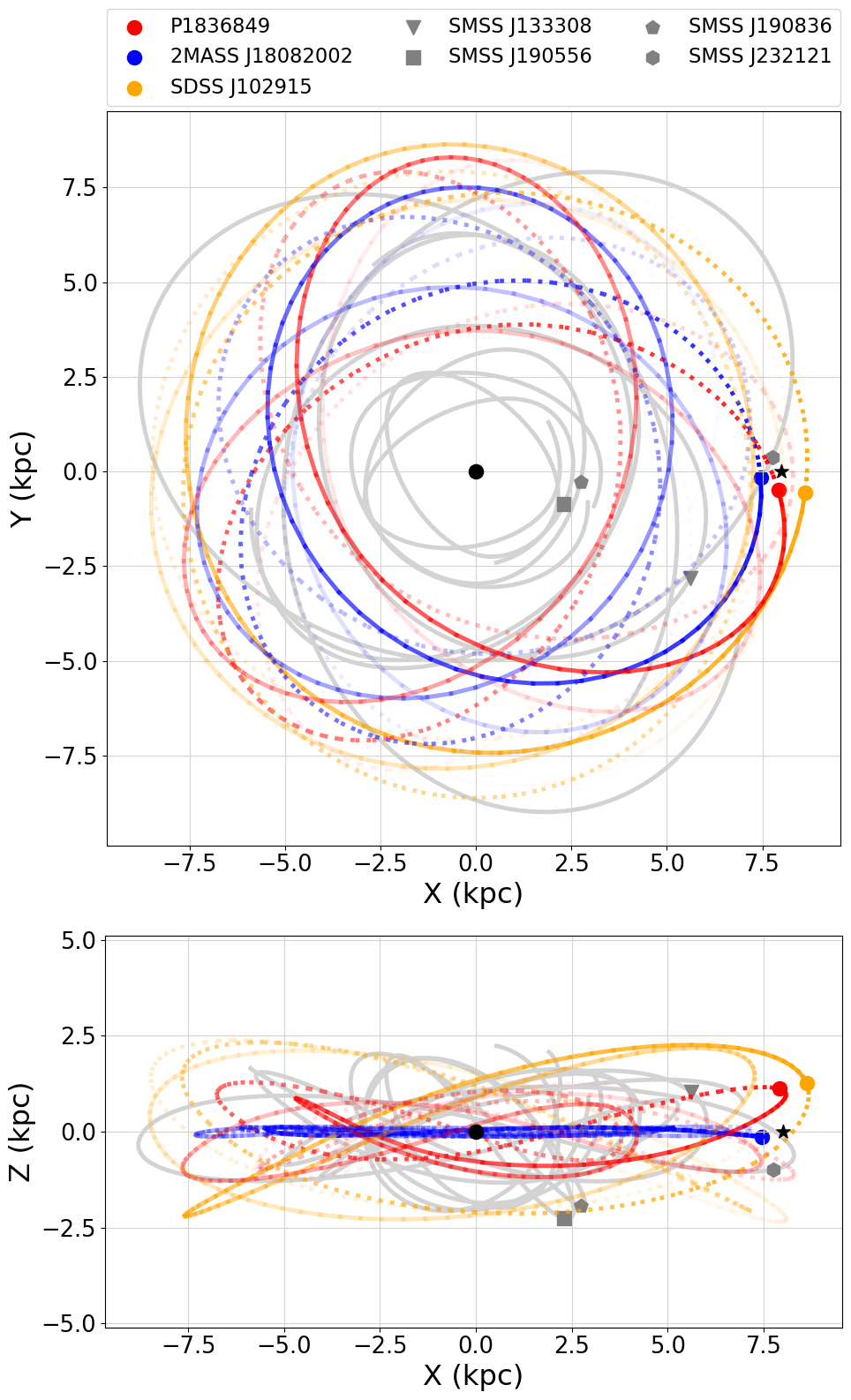
Figure 2: Galactic orbital motion. Top panel: Galactic Y vs. X. Bottom panel: Galactic Z vs. X. The positions at the present time of P1836849, SDSS J102915, and 2MASS J18082002 are marked by the red, orange, and blue circles, respectively. Solid and dotted lines of similar colour denote the orbits integrated backwards and forwards. The orbits for the four SkyMapper stars are shown in grey (solid lines only, though their orbits are also integrated backwards and forwards). Their current positions are noted as grey symbols. Black circle and black star mark the position of the Galactic centre and of the Sun.

3.2 Orbital parameters

The 6D kinematic data for P1836849 has been updated from Gaia DR2 to Gaia DR3 values, including the new astrometric distance, and the new RV determined from the GHOST spectrum (see Table 3). Orbital parameters are derived using galpy (Bovy, 2015), where the same Galactic gravitational potential as in Sestito et al. (2019) and Venn et al. (2020) has been adopted. This briefly consists in the MWPotential2014 with an increased dark matter halo mass of $1.2\times 10^{12}\rm M_{\odot}$ (Bland-Hawthorn & Gerhard, 2016). Uncertainties on the orbital parameters are derived from a Monte Carlo simulation on the input parameters (distance, RV, proper motion, coordinates), drawing them from Gaussian distributions for 1000 times. Then, the median and the standard deviation are used to represent the measurement of a parameter and its uncertainty. Present and previous orbital parameters are listed in Table 3. The apocentric distance and the maximum height from the plane are in agreement within less than $1\sigma$ from the previous measurements. The new pericentric distance is smaller than previously inferred, resulting in a slightly higher eccentricity. In both cases, the star has a prograde motion.

As a comparison, the orbital parameters of SDSS J102915 and of 2MASS J18082002 are also re-derived using Gaia DR3 and the methods described above; summarised in Table 3. These two stars were found in a very similar kinematical configuration as of our target (Schlaufman et al., 2018; Sestito et al., 2019; Mardini et al., 2022a). The updated apocentric and pericentric distances of SDSS J102915 are now smaller than previously inferred with Gaia DR2 (Sestito et al., 2019), and these updates have only small effects on the orbit eccentricity and its maximum height from the plane. The updates for 2MASS J18082002 result in a smaller pericenter and larger eccentricity (Schlaufman et al., 2018; Sestito et al., 2019), also seen by Mardini et al. (2022a), and its orbit has a remarkably small maximum height from the plane ($\sim 0.13{\rm\,kpc}$). The new Galactic orbits for the three stars are shown in Figure 2, integrating forwards and backwards by 0.5 Gyr each.

Finally, we add the four SkyMapper stars to Figure 2, using their Gaia DR3 positions and proper motions in our potential, with distances and radial velocities from Cordoni et al. (2021). For clarity, all four orbits are marked with grey solid lines, but their orbits are also integrated backwards and forwards by 0.1-0.2 Gyr each (for clarity). Only one of the SkyMapper stars is near the main-sequence (SMSS J232121, a sub-giant), placing it in the solar neighbourhood at present, similar to P1836849, SDSS J102915, and 2MASS J18082002.

3.3 Stellar parameters

A first estimate of the effective temperature (T_eff) for P1836849 was determined using the colour-temperature relation for Gaia photometry from Mucciarelli, Bellazzini & Massari (2021). This calibration was selected based on their inclusion of very metal-poor stars (from González Hernández & Bonifacio, 2009) and has been very successful when applied to the analyses of extremely metal-poor stars (e.g.,  Kielty et al., 2021; Waller et al., 2023; Sestito et al., 2023b). A first estimate of the surface gravity (log $g$) is determined using the Stefan-Boltzmann equation (e.g., see Venn et al., 2017; Kraft & Ivans, 2003) and assuming the first estimate on T_eff. These estimates were iterated several times for a convergence on the final T_eff and log $g$ (see Sestito et al., 2023b, for a full description). Uncertainties are derived with a Monte Carlo simulation, drawing all the input parameters (distance, G, BP$-$RP, A_V, [Fe/H] - as well as the correlated uncertainties of T_eff and logg) from a Gaussian distribution for $10^{5}$ times. A flat mass distribution between 0.5 to 0.8 ${\rm\,M_{\odot}}$ is assumed in the surface gravity uncertainty. A 10% uncertainty in extinction is adopted throughout.

Stellar parameters and uncertainties for P1836849 are reported in Table 3. These new stellar parameters are within the $1\sigma$ errors of the previous estimates by Venn et al. 2020. However, the uncertainties on the effective temperature are larger compared to the previous estimates based on isochrones. This is a concomitance of two effects. The first is that methodologies based on isochrones can underestimate the intrinsic systematic errors in the theoretical models. The second is due to the photometric temperature calibration itself, where Sestito et al. (2023b) showed that the large uncertainty only occurs for the hotter stars in the upper main sequence and the sub-giant branch. Microturbulence ($\xi=1.3{\rm\,km\ s^{-1}}$) was adopted from the calibrations for metal-poor dwarfs by (Sitnova et al., 2015).

Effective temperatures and surface gravities were also re-determined for SDSS J102915 and 2MASS J18082002. For SDSS J102915, the updated stellar parameters are in agreement with the inference based method using Gaia DR2 (Sestito et al., 2019), confirming the star is a dwarf. For 2MASS J18082002, the temperature is now in agreement with the values from Mardini et al. (2022a) and Schlaufman et al. (2018), while the surface gravity confirms its sub-giant nature.

4 Spectral Line Analyses

Chemical abundances in P1836849 were determined from individual spectral lines. Spectral lines were selected from the recent GRACES and ESPaDoNS analyses of metal-poor halo stars (Venn et al., 2020; Kielty et al., 2021; Lucchesi et al., 2022), and updated with a search of the P1836849 GHOST spectrum for additional lines from spectrum syntheses (described below). All atomic data and additional spectral lines were taken from the recent version of linemake atomic and molecular line database (Placco et al., 2021), see Tables 5 and 6. We note that hyperfine structure (HFS) components were only significant for our results for two spectral lines: Sc ii 4246.822 Å and Mn i 4030.746 Å.

Chemical abundances have been determined from a classical model atmospheres analysis using the stellar parameters in Table 3. Model atmospheres are from MARCS (Gustafsson et al., 2008), and we restrict the analysis to relatively unblended and weak spectral lines (i.e., equivalent width EW $<130$ mÅ). Chemical abundances are compared to the Sun using standard notation, and solar abundances from Asplund et al. (2009).

4.1 Spectrum Syntheses

The 1D LTE radiative transfer code MOOG (Sneden, 1973; Sobeck et al., 2011) was used to synthesise the stellar spectra using the stellar parameters as described above. This method was carried out in three steps: (1) a model atmosphere was generated with the initial parameters: T_eff, log $g$, and $\xi$ as described in Section 3, and an initial metallicity of [Fe/H]$=-3.2$. The iron lines were synthesised for a preliminary metallicity estimate, and the model atmosphere updated with the new metallicity. This process was repeated until the metallicity output matched the input (typically only twice). (2) A new synthesis of all elements was generated which included line abundances and upper limits for all of the clean spectral lines. (3) NLTE (below) and HFS corrections were applied. Each synthetic spectrum was broadened in MOOG to match the observed spectrum; we found that a Gaussian smoothing kernel with FWHM $=0.17$ was a good match to the GHOST spectral resolution and internal thermal broadening for this main sequence star. If the spectral features were well fit, then we calculated an abundance for that line from the syntheses. If not, then a 3$\sigma$ maximum equivalent width was used to calculate an upper limit on the abundances (i.e., this was applied to Na, Sr, Ba, and Eu). This method was also used to synthesise the CH molecular feature near 4300 Å  (see Section 5.1 for details).

4.2 Checking the stellar parameters

It is possible to check the stellar parameters from spectroscopic features, in particular; a flat distribution of A(Fe i) as a function of (i) excitation potential ($\chi$) indicates an appropriate effective temperature, (ii) wavelength indicates appropriate sky subtraction and data reduction, (iii) line strength indicates an appropriate microturbulence value ($\xi$), and (iv) an ionisation balance between Fe i and Fe ii is typically employed to determine the optimal surface gravity.

Our analysis of P1836849 found a slope d[A(Fe i)/$\chi$] $<0.1$ dex eV^-1, which falls well within 1$\sigma$ of the [Fe i/H] measurements. A similar result was obtained even after applying NLTE corrections, thus confirming our adopted T_eff. No statistically significant slope was found for A(Fe i) vs wavelength or line strengths. The latter confirms our microturbulence value, which was set from the empirical relation for cool dwarfs from Sitnova et al. (2015) that depends on surface gravity - however, our surface gravity value itself is less certain, as [Fe i/H] = [Fe ii/H] +0.2 (LTE) or +0.3 (NLTE). Recent findings by Karovicova et al. (2020) indicate that A(Fe i) can deviate by as much as +0.7 dex from A(Fe ii) in very metal-poor red giants, but only approximately $+0.1\pm 0.1$ dex for EMP dwarf stars, like P1836849. Thus, our offset of +0.2 to +0.3 dex based on only a few A(Fe ii) lines seems reasonable, and we refrain from adjusting the surface gravity values any further. We consider our stellar parameters to be appropriate.

Table 4: Averaged LTE and NLTE chemical abundances, and final total uncertainty $\sigma$ (which has been divided by the square root of the number of lines N). NLTE corrections are from the following References: (a) Lind, Bergemann & Asplund (2012), (b) Lind et al. (2011), (c) Bergemann et al. (2017), (d) Bergemann et al. (2013), (e) Mashonkina et al. (2017), (f) Bergemann (2011), (g) Bergemann & Cescutti (2010), (h) Bergemann et al. (2019), (i) Nordlander & Lind (2017). *Fe species are [X/H] instead of [X/Fe].

Species	[X/Fe]	$\sigma$	N	[X/Fe]	REF
	LTE			NLTE
Fe i*	$-3.22$	$0.05$	39	$-3.08$	a
Fe ii*	$-3.42$	$0.11$	3	$-3.41$	a
CH	$<+0.80$	$-$	$-$	$-$	$-$
Na i	$<-0.62$	$0.15$	3	$<-0.80$	b
Mg i	$0.05$	$0.11$	4	$0.03$	c
Al i	$-0.60$	$0.15$	1	$-0.23$	i
Si i	$0.25$	$0.15$	1	$0.22$	d
Ca i	$0.05$	$0.12$	1	$0.20$	e
Sc ii	$0.24$	$0.15$	1	$-$	$-$
Ti ii	$0.58$	$0.12$	7	$0.51$	f
Cr i	$0.07$	$0.12$	2	$0.50$	g
Mn i	$-0.08$	$0.15$	1	$0.41$	h
Ni i	$0.30$	$0.15$	1	$-$	$-$
Sr ii	$<-0.10$	$-$	2	$-$	$-$
Ba ii	$<-0.50$	$-$	1	$-$	$-$
Eu ii	$<+3.40$	$-$	1	$-$	$-$

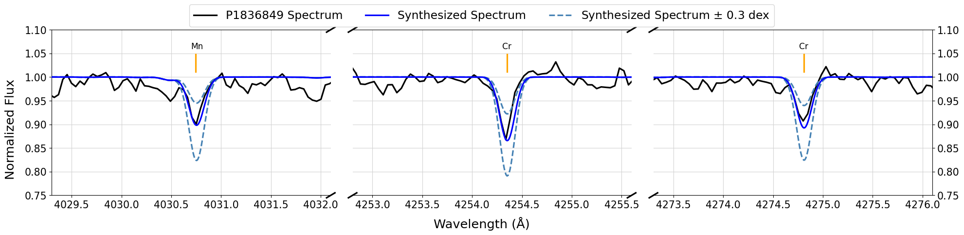
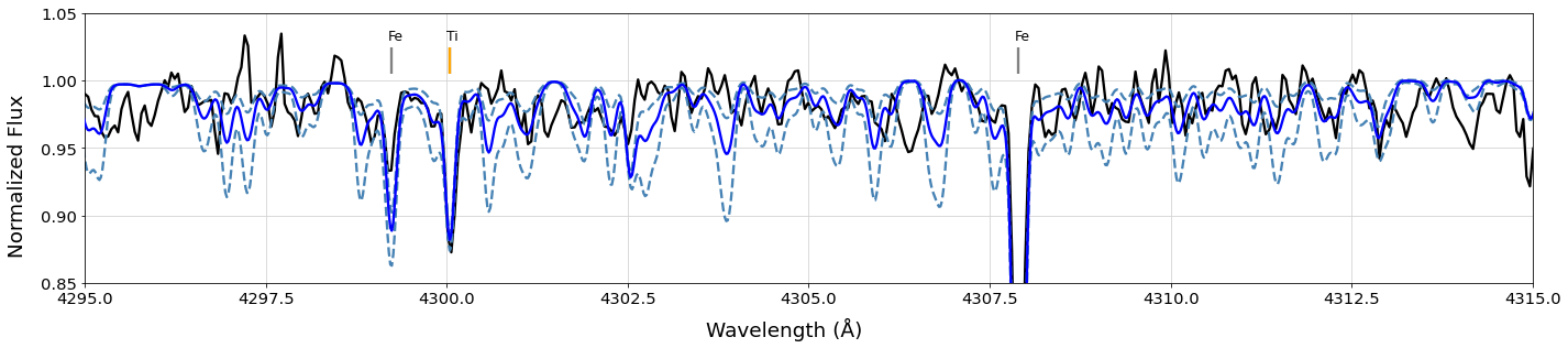
Figure 3: Upper Panels: The Mn i and two Cr i lines used in this analysis are shown, including our best fit syntheses, and $\Delta$[X/Fe] $\pm 0.3$. Though the lines are weak ($\lesssim 30$ mÅ each), they are clear and well modelled. Lower Panel: The G-band including our best upper-limit syntheses, with ¹²C/¹³C$=40$ (EMP dwarf, e.g., Spite, Spite & Barbuy 2021) and [C/Fe]$=+0.8$. Two more syntheses show $\Delta$[C/Fe]$\pm 0.3$. One Ti ii line used in this analysis (orange) and two Fe i lines not used (grey) are also indicated. The plot is zoomed in for clarity.

5 Chemical abundances analysis

The wavelength coverage of GHOST allows us to observe spectral lines of carbon, $\alpha$-, odd-Z, Fe-peak, and neutron-capture process elements. In total, 61 spectral features are measured in this analysis of P1836849, which is significantly more than the nine lines in total analysed by Venn et al. (2020). A search for additional clean, unblended spectral lines did not produce any more suitable for an abundance analysis. The chemical abundances and uncertainties are presented in Table 4.

5.1 Carbon

Carbon was examined from spectrum synthesis of CH near 4300 Å using the updated molecular line list from Masseron et al. (2014) available in linemake. We also adopted ¹²C/¹³C$=40$ based on the recent finding for the EMP subgiant HD 140283 (Spite, Spite & Barbuy, 2021). We found no evidence for a carbon enrichment, with an upper-limit of [C/Fe] $<+0.8$; see Fig. 3 (note that the wing of H$\gamma$ extends to this region and has been removed in both the observed and synthetic spectra for this plot). Examination of the N and O abundances showed negligible effects. Changes in the isotopic ratio of $\Delta$(¹²C/¹³C)$\pm 10$ resulted in $\Delta$[C/Fe]$=\mp 0.1$. Due to the high temperature and gravity of this star, our non-detection of carbon is primarily due to the feasibility of the line formation itself, and not the SNR of the GHOST spectrum.

5.2 $\alpha$-elements

The $\alpha$-elements with detectable spectral lines in P1836849 are Mg i (4), Si i (1), Ca i (1), and Ti ii (7). The A(Mg i) is an average of the abundances from 2 lines of the Mg i Triplet ($\lambda\lambda 5172.68,5183.60$ Å, the third line is blended with iron and ignored) and 2 lines in the blue spectrum (at 3829.35 Å and 3832.30 Å). The latter two lines are amongst the strongest lines in our analyses, and Mg i 3832.30 Å is in a noisy region of spectrum, yet both have EW $\lesssim 130$ mÅ and are not extremely sensitive to the microturbulence ($\xi$) values, thus we have kept them in our analysis. Only one line of Si i is detected at $3905.52$ Å. Similarly, only the resonance line of Ca i at $4226.72$ Å was detected, both sufficiently weak and in a clean spectral region. We do not include an analysis for calcium of the strong Ca ii Triplet, as each line has EW $\gtrsim 150$ mÅ. Ti ii was observable from 7 weak spectral lines ranging between $3913.4$ and $4571.9$ Å.

5.3 Odd-Z elements

The abundances of odd-Z elements have a strong dependence on the metallicities of their progenitors, seen as a strong odd-even effect in low metallicity stars (e.g., Nomoto, Kobayashi & Tominaga, 2013). We were able to measure only two spectral lines of odd-Z elements; Al i 3961.52 Å and Sc ii 4246.82 Å. The former is shown in Figure 1 and the latter spectral feature has hyperfine structure that is included in our spectrum synthesis analysis. We also examined the Na i Doublet ($\lambda\lambda 5889.95$ and 5895.92 Å), but could not clearly detect the lines. As shown in Figure 1, there is significant telluric contamination near the Na d feature as this target (DEC=+5^o) was observed through a high airmass at Gemini-South (strong atmospheric bands can also be seen from 6900 to 8400 Å). A re-examination of the ESPaDOnS spectrum taken at lower air mass at the CFHT (Northern hemisphere; Venn et al., 2020) also suggests that the Na d lines in P1836849 are in the noise, and absent when compared to our standard star HD 122563. We use the GHOST spectrum to determine an upper-limit for sodium in P1836849; using both spectrum synthesis and a maximum (3$\sigma$) equivalent width EW = 13 mÅ, we find [Na/Fe]${}_{NLTE}<-0.8$.

5.4 Fe-peak elements

The Fe-peak elements observable in our GHOST spectrum include Fe i (39), Fe ii (3), Cr i (2), Mn i (1), and Ni i (1). This is a significant increase compared to Venn et al. (2020) where only 2 lines each of A(Fe i) and A(Fe ii) were available - all 4 were re-analysed in our GHOST spectrum. Our final iron abundance for P1836849 is [Fe/H]$=-3.3\pm 0.1$, which is the (unweighted) average of our Fe i and Fe ii results in Table 4, in both LTE and NLTE. New Fe-peak spectral lines include the two Cr i resonance lines detected at $\lambda$4254.35 and $\lambda$4274.81 Å, and the Mn i resonance line at $\lambda 4030.74$ Å; these features and our spectrum syntheses are shown in Figure 3. We note that the Mn i exhibits hyperfine structure taken into account in our spectrum synthesis. A weak Ni i line is also detected at $3858.29$ Å.

5.5 Neutron-capture elements

The high-quality blue spectral coverage of the GHOST spectrograph opens new possibilities for the detection and precision measurements of neutron-capture elements in metal-poor star. However, our target P1836849 does not include any of the heavy elements as it is too warm and not r-process rich. We calculate upper-limits only on the abundances of Sr, Ba, and Eu. While our non-detections for the Sr ii 4077.70, 4215.51 Å, and Ba ii 4554.03 Å  resonance lines provide interestingly low upper-limits ([Sr/Fe] $<-0.1$, [Ba/Fe] $<-0.5$), the Eu ii 4129 Å upper-limit does not provide a useful constraint ([Eu/Fe] $<+3.4$; hyperfine structure and isotopic components are included in this spectrum synthesis).

5.6 Non-Local Thermodynamic Equilibrium corrections

The radiation field in the atmospheres of EMP stars contributes to significant non-local thermodynamic equilibrium (NLTE) effects, which can be large for some species. NLTE corrections have been applied whenever possible, using corrections tabulated in the MPIA data base. For Na i and Fe ii, we use corrections available in the INSPECT database, and for Al i, we apply NLTE corrections from Nordlander & Lind (2017). References for the NLTE corrections for individual elements are also in Table 4. 1D LTE and NLTE abundances are shown in Figures 4 and 5.

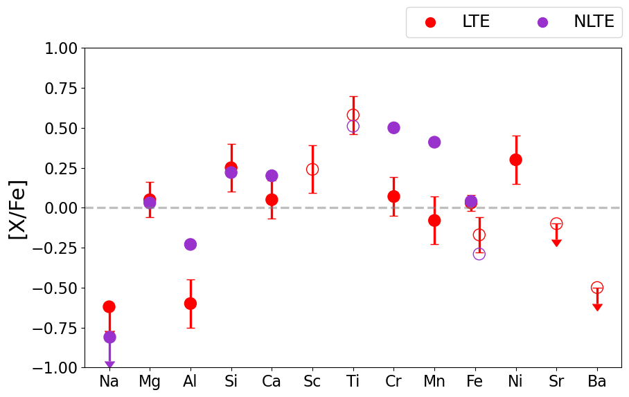
Figure 4: P1836849 LTE (red) and NLTE (purple) chemical abundances compared to solar. Filled points are for neutral species, while open circles are for singly-ionized species. Error bars are shown for LTE abundances only.

5.7 Chemical abundance uncertainties

In Table 4, we report the chemical abundance ratios from our 1DLTE analysis as [X/Fe]_LTE. The total error $\sigma_{\rm A(X)}$ includes the effects due to uncertainties in the stellar parameters ($\delta_{\rm T_{eff}}$, $\delta_{\rm logg}$), added in quadrature with the measurement errors. Measurement errors due to continuum placement and SNR are computed per line, and combined per species such that $\delta_{\rm X}=\delta_{\lambda}/\sqrt{{\rm N_{X}}}$.

6 Discussion

The chemistry of P1836849 is compared directly to solar and scaled-solar abundances (reduced by [Fe/H]$=-3.3$) in Fig. 4 and Fig. 5. Regardless of whether the LTE or NLTE abundance ratios are examined, P1836849 is not similar to the Sun - particularly the very low ratios of Na, Al, and Ba, as well as the high ratios of Ti, Ni and the NLTE-corrected values of Cr and Mn. It is clear that P1836849 formed in a region with a very different star formation history and chemical evolution than that of the Sun.

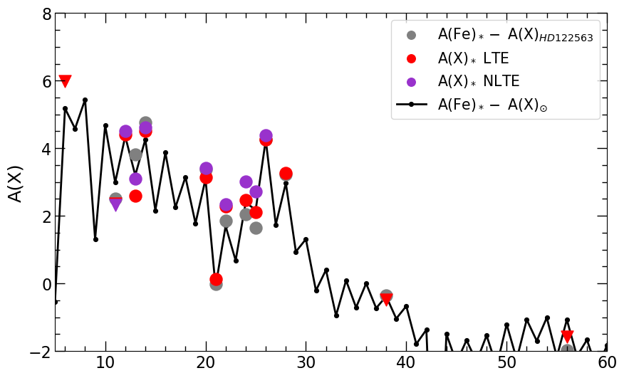
Figure 5: P1836849 LTE (red) and NLTE (purple) chemical abundances vs atomic number compared to scaled-solar abundances ($\Delta$[Fe/H] $=-3.3$), including upper limits (downward triangles) for C, Na, Sr, & Ba.

6.1 Comparison with MW disk stars

The majority of known stars with planar kinematics have metallicities [Fe/H]$>-2$. A detailed homogeneous survey of the chemical elements in these stars (Bensby, Feltzing & Oey, 2014; Battistini & Bensby, 2015, 2016) describes the chemical enrichment of the MW thin and thick disks in terms of yields from SN II (for stars with [Fe/H]$<-0.4$) and the later contributions from SN Ia and AGB stars. In Fig. 6, we show [Mg/Fe] for these disk stars (black markers), as well as those available in the Sloan Digital Sky Survey Data Release 17 (Abdurro’uf et al., 2022a) from the Apache Point Observatory Galactic Evolution Experiment (APOGEE, Majewski et al., 2017) (grey markers). The APOGEE stars were selected to have |Z|$<$3 kpc, and space velocities $150<$ V${}_{\phi}<250{\rm\,km\ s^{-1}}$, and |V_R| and |V_Z| $<30{\rm\,km\ s^{-1}}$ (Queiroz et al., 2020; Gaia Collaboration et al., 2021, calculated using APOGEE radial velocities, STARHORSE distances, and Gaia EDR3 proper motions). Clearly, P1836849 does not resemble the stars that describe the MW disk, nor belong to a population extrapolated to very low metallicities of either the thin or thick disk stars.

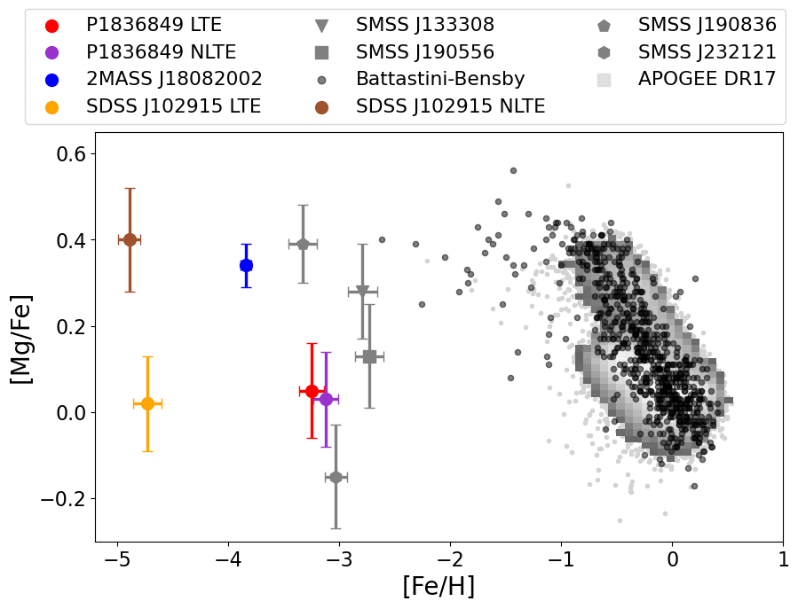
Figure 6: LTE [Mg/Fe] vs [Fe/H] for stars in the Galactic disk(s) from Bensby, Feltzing & Oey (2014), Battistini & Bensby (2015, 2016), and selected from APOGEE DR17 (Abdurro’uf et al., 2022b, see text). The EMP stars with high resolution spectroscopic abundances and prograde quasi-circular planar orbits from Fig. 2 and Table 3 are also shown. The NLTE abundances for P1836849 and SDSS J102915 are also shown.

6.2 Comparison with EMP planar stars

We compare the chemistry and kinematics of P1836849 with the six other known EMP stars with prograde quasi-circular planar orbits that currently have detailed chemical abundances from high resolution spectroscopy: see Tables 1 and 3. Their orbits are shown in Fig. 2, and, at first glance, look quite similar. However, upon closer examination, the eccentricities vary by a factor of $\sim 4$, and two of the SkyMapper stars have quite small apocentric distances. The minimum eccentricity is that of SDSS J102915 ($\epsilon\sim 0.09$) and the maximum is that of P1836849 ($\epsilon\sim 0.38$) Furthermore, the orbit of SDSS J102915 reaches a maximum height of $\sim 2.2{\rm\,kpc}$, a factor of two larger than P1836849, and much larger than the very flat orbit of 2MASS J18082002.

The LTE abundances of these stars are compared in Fig. 7; LTE abundances are compared as NLTE corrections were not applied in the other analyses. Unfortunately, the stellar parameters of these seven stars are not very similar; P1836849 is hotter than the comparison stars by $>$800 K, two comparison stars are subgiants rather than dwarfs, and three of the SkyMapper stars are red giants. Furthermore, SDSS J102915 and 2MASS J18082002 are more metal-poor than P1836849 by $\gtrsim 1.0$ dex; see Table 3. These differences impact our ability to directly compare their abundances as systematic errors are not well constrained. Nevertheless, some of the chemical abundances are similar between P1836849 and SDSS J102915, e.g., $\alpha$-elements (other than Ti). The same is not true when the stellar chemistries are compared with 2MASS J18082002 and the four SkyMapper stars, which has very different abundances for Na, Cr, Mn, and possibly Al, Sc, and Ti.

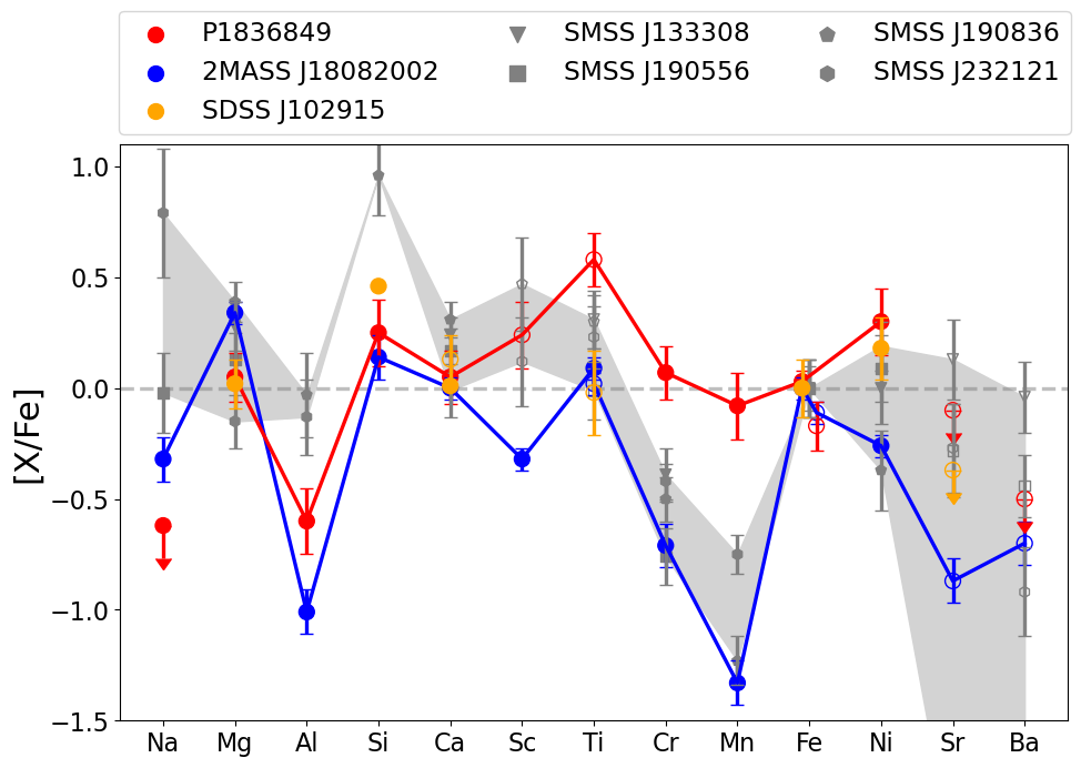
Figure 7: A comparison of the LTE stellar abundances in P1836849 (red; this paper), SDSS J102915 (orange; Caffau et al., 2011, 2012), 2MASS J18082002 (blue; Schlaufman et al., 2018; Mardini et al., 2022b), and the four SkyMapper stars (gray; Yong et al., 2021). Gray shading connects the highest and lowest values amongst the SkyMapper stars, for clarity. P1836849 appears to be chemically distinct from the comparison stars, and a wide range in abundances is seen for the whole sample.

Were these stars born in the same formation site? It seems unlikely, despite some chemical and/or dynamical similarities discussed above. Furthermore, if they have been orbiting the MW since the early Galactic assembly, we can expect that they would have experienced many perturbations over cosmic time (e.g., Gaia-Sausage-Enceladus, Belokurov et al. 2018; Helmi et al. 2018), which could have heated or altered their orbital configurations (e.g.,  Navarro et al., 2018; Di Matteo et al., 2019). Their orbits may also have been affected by secular and non-linear interactions between the rotating MW bar and its spiral arms (Minchev & Famaey, 2010; Sestito et al., 2020). An investigation into a common origin for EMP stars on prograde quasi-circular orbits in the Galactic plane will require larger statistical samples than presented here.

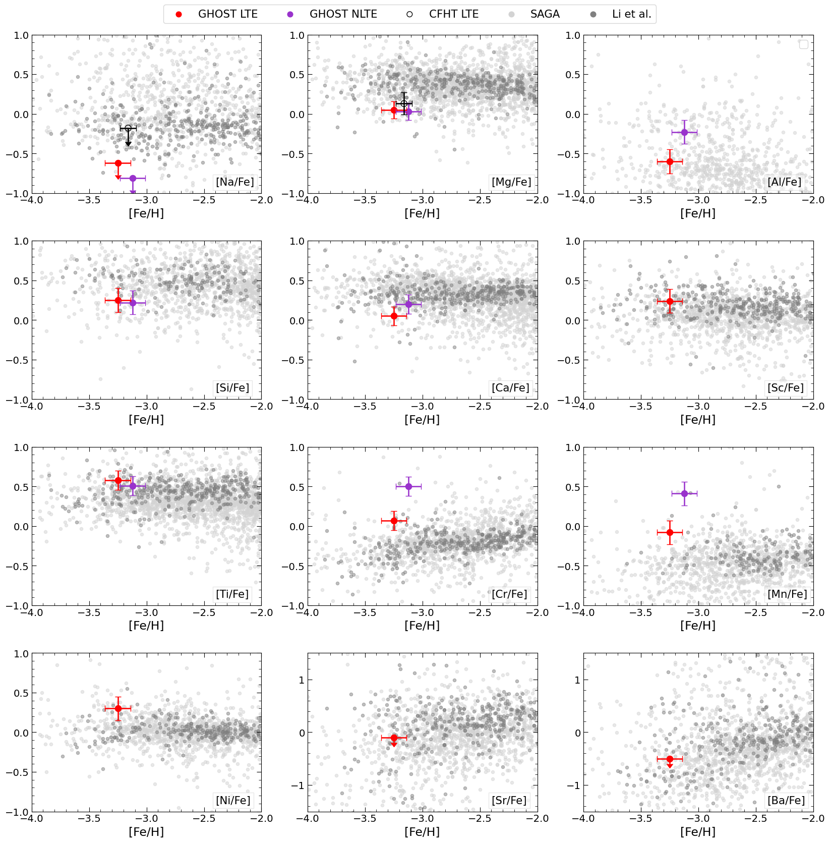
Figure 8: Chemical abundances of P1836849 compared with metal-poor stars in the MW (halo) from the homogeneous high-resolution spectroscopic study by Li et al. (2021, dark gray markers) and other stars in the SAGA database (Suda et al., 2008, and references within) (light gray markers). Red and purple symbols represent our LTE and NLTE-corrected abundances for P1836849, respectively.

6.3 Comparisons with other EMP stars in the MW halo, Sculptor, and UFD galaxies

The chemical abundances of P1836849 are compared to a compilation of stars of similar metallicity in the MW halo in Fig. 8. This includes chemical abundances of stars gathered from the literature in the Stellar Abundances for Galactic Archaeology database (SAGA, light grey circles; Suda et al., 2008), and the high-resolution spectroscopic dataset taken with HDS at the Subaru Telescope and analysed homogeneously by Li et al. (2022, dark grey circles). It is clear that the chemistry of P1836849 does not resemble the majority of EMP stars in the MW halo. For example;

• The [Na/Fe] upper limits found for P1836840 are extremely low compared to nearly all MW halo stars, in both LTE and NLTE.

• The $\alpha$-elements (Mg, Si, Ca) are only consistent with the lowest values found in the MW halo stars.

• The Cr and Mn abundances are higher than the majority of the MW halo stars, and very high after NLTE corrections are applied.

These are unlikely due to systematic errors in the NLTE corrections, as many of the halo stars are nearby F and G dwarfs with small to negligible NLTE corrections for most of their spectral lines.

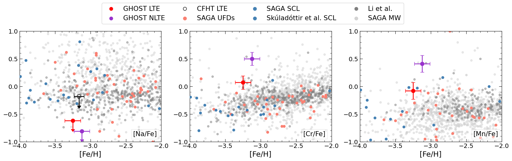
Figure 9: A comparison of [Na/Fe], [Cr/Fe], and [Mn/Fe] of P1836849 to stars in the MW (symbols and sources same as in Fig. 8), to stars in the UFD galaxies as summarized in the SAGA database (Suda et al., 2017, salmon markers; see text), and to stars in the classical dwarf galaxy Sculptor from both the SAGA database and Skúladóttir et al. (2023) (steelblue markers; see text). We note that the majority of the abundance ratios shown here have not been corrected for NLTE effects.

The chemistry of P1836849 can also be compared to EMP stars in nearby dwarf galaxies. As an example, in Fig. 9 we compare our results to a sample of homogeneously analysed EMP stars in the classical (’textbook’) dwarf galaxy Sculptor (e.g., Hill et al., 2019; Skúladóttir et al., 2023). The $\alpha$-elements in Sculptor are slightly lower than EMP stars in the MW halo, which is typical of dwarf galaxies and has been discussed in terms of the slower star formation history of low mass satellites (Venn et al., 2004, 2012; Tolstoy, Hill & Tosi, 2009; Jablonka et al., 2015; Hill et al., 2019). Thus, the [$\alpha$/Fe] ratios in P1836849 are more similar to the EMP stars in Sculptor (not shown); however, P1836849 still stands out in Na and the iron-peak elements, as shown in Fig. 9. Note that we have included additional stars in Sculptor from the SAGA database (Suda et al., 2017), however most of those have [Fe/H]$>-2.5$.

Our results for P1836849 are also compared to EMP stars in the UFD galaxies collected in the SAGA database by Suda et al. (2017, and references therein). This includes EMP stars in BooI, BooII, CVnI, CVnII, Com, GruI, Her, Hor, LeoII, LeoIV, LeoT, PscII, RetII, Seg1, Seg2, TriII, TucII, TucIII, UMaII, & WilI. As seen in Fig. 9, again, the only elements that stand out in P1836849 are Na, Cr, and Mn when compared to the EMP stars in the UFDs.

Thus, in general;

• The [Na/Fe] upper limits found for P1836840 are much lower than the EMP stars in Sculptor and the majority of EMP stars in the UFDs.

• The LTE and NLTE Cr abundances are higher than for the stars in Sculptor ($\gtrsim$0.5 dex) and in UFDs ($\gtrsim$0.2 dex).

• The Mn (and possibly Ni, not shown) abundances are higher than the majority of the comparison stars in Sculptor and the UFDs. A homogeneous analysis of Mn i with NLTE corrections may be necessary to further compare these stellar populations.

Finally, we note that Skúladóttir et al. (2021, 2023) suggest that one EMP star AS0039 in Sculptor has a chemical abundance pattern that resembles enrichment from theoretical yields of a zero-metallicity hypernova progenitor (of mass M = 20M_⊙), solidifying this galaxy as a benchmark for understanding the first supernovae in the Universe. In the next section, we compare P1836849 to theoretical yields from Population III supernovae.

6.4 StarFit result

To examine if the chemical abundance ratios in P1836849 could be reproduced by the predicted nucleosynthetic yields from Population III supernovae (SNe) and hypernovae (HNe), our LTE and NLTE abundances are compared to theoretical yields from Heger & Woosley (2010) and Heger et al. (2012) using the web version of StarFit (v0.19.1). These models predict the nucleosynthetic products of massive metal-free stars, without mass loss or rotation, and with a range of explosion energies and mixing fractions. The fallback models (S4) used in this work have masses from 10 to 100 M_⊙, explosion energies ranging from 0.3 x 10⁵¹ erg to 10⁵² erg, and a range of mixing prescriptions. StarFit can be used to search for a single SN or HN progenitor or a combination of SNe and HNe, providing a $\chi^{\rm 2}$ for the best fit to the observed abundances. This algorithm has been applied successfully to EMP stars in the literature (e.g., Placco et al., 2016, 2020; Nordlander et al., 2017; Skúladóttir et al., 2021)

At first, the StarFit solutions to the chemistry of P1836849 appeared to be poorly constrained, due to insufficient chemical data, especially for the neutron-capture elements. StarFit either struggled to converge, produced a range of models with satisfactory fits, or failed to converge to the same solution after repeated trials with the same input parameters. To improve the application of StarFit, we reduced the search parameters to only 1-3 SNe and/or HNe from the updated fallback models by Heger et al. (2012), and only fit the data from H to Ni using the Genetic Algorithm and a 60 second time limit. Our best fit to the NLTE abundances for P1836849 is shown in Fig. 10, which includes a 10.2 M_⊙ SN model with explosion energy B = 1.8 x 10⁵¹ erg and mixing parameter log($f_{\rm mix}$)$=-1.4$ from the S4 models combined with a 17.1 M_⊙ HN model with higher explosion energy B = 10.0 x 10⁵¹ erg and the same mixing parameter from the Ye models. This fit provides a $\chi^{2}$=0.94, compared to either model (or other single models) independently, where $\chi^{2}>2$. We note that the high abundances of Cr and Mn in our results are produced by the HN event, i.e., from incomplete Si-burning layers.

This result is consistent with the analyses by Skúladóttir et al. (2021, 2023) for EMP stars in Sculptor (see Section 6.3), and also Ishigaki et al. (2018, 2014) who found that the abundance patterns of $\sim$200 EMP stars in the MW halo are best-fit by SN with mass $<$40 M_⊙ and/or HN with mass =25 M_⊙. This result led them to suggest that the masses of the first stars responsible for the early metal enrichment in the Galaxy were not extremely high, either because high-mass first stars were rare, they directly collapsed into a black hole without ejecting heavy elements, or supernova explosions from higher-mass Population III stars may have inhibited their formation. Studies of EMP stars in other nearby galaxies, and old EMP stars in the MW, can address these options, i.e., where kinematic information in target selection may help in the future.

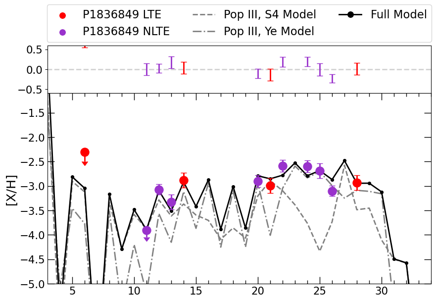
Figure 10: P1836849 LTE (red) and NLTE (purple) chemical abundances vs atomic number compared to our best StarFit model (see text), which includes a low mass Pop III supernova (10 M_⊙, S4 models) and a low mass Pop III hypernova (17 M_⊙, Ye models). NLTE abundances were used whenever possible, and LTE abundances are shown for the remaining elements, with 1$\sigma$ residuals from the model shown across the top.

7 Conclusions

As part of the commissioning of the new Gemini High-resolution Optical SpecTrograph (GHOST), we have observed an EMP star with a prograde quasi-circular orbit in the Galactic plane, Pristine_183.6849+04.8619 (P1836849), during the Science Verification stage. The exquisite throughput of GHOST has enabled a detailed spectral analysis of features from 3700 - 11000 Å of many chemical elements (Mg, Al, Si, Ca, Sc, Ti, Cr, Mn, Fe, Ni), and has provided valuable upper limits for others (Na, Sr, Ba). This star is extremely metal-poor ([Fe/H]=-3.3$\pm$0.1) compared to other stars with MW planar orbits, and shows unusually low [Na/Fe] and high [Cr/Fe] and [Mn/Fe] compared with other EMP stars in the MW halo, Sculptor, and UFD galaxies. A simple comparison of our NLTE abundances to theoretical yields from supernova models suggests that only two low mass Population III objects are needed to reproduce the abundance pattern: one 10 M_⊙ supernova and one 17 M_⊙ hypernova (reduced $\chi^{2}<1$). Our analysis of P1836849 contributes to the growing evidence that the earliest stages of chemical enrichment in the Universe were dominated by low mass Population III supernovae and hypernovae.

Data Availability

GHOST Science Verification spectra are available at the Gemini Archive web page https://archive.gemini.edu/searchform. All data are incorporated into the article.

8 Appendix A: Line Lists

Table 5: Iron line list. The source and quality of the atomic data is provided as Q, where A= OBR91 ($<$10%), B= NIST C (25%), C= NIST D+ (50%) precision. NLTE corrections ($\Delta$) are from the MPIA database.

$\lambda$	Elem	$\chi$	log(gf)	Q	A(X)	$\Delta$
(Å)		(eV)			LTE	NLTE
3758.233	26.0	0.957	-0.01	A	4.07	0.13
3763.789	26.0	0.989	-0.22	A	4.22	0.14
3787.880	26.0	1.010	-0.84	A	4.37	0.14
3815.840	26.0	1.484	0.24	A	4.42	0.14
3820.425	26.0	0.858	0.16	A	4.32	0.10
3824.444	26.0	0.000	-1.34	A	4.72	0.14
3825.881	26.0	0.914	-0.02	A	4.27	0.11
3827.823	26.0	1.556	0.09	A	4.22	0.14
3840.438	26.0	0.989	-0.50	A	4.22	0.14
3841.048	26.0	1.607	-0.04	A	4.27	0.14
3849.967	26.0	1.010	-0.86	A	4.27	0.12
3856.372	26.0	0.052	-1.28	A	4.62	0.14
3859.912	26.0	0.000	-0.70	A	4.77	0.12
3878.018	26.0	0.957	-0.90	A	4.27	0.14
3878.573	26.0	0.087	-1.38	A	4.47	0.14
3895.656	26.0	0.110	-1.67	A	4.37	0.14
3902.946	26.0	1.556	-0.44	A	4.22	0.14
3920.258	26.0	0.121	-1.73	A	4.52	0.14
3922.912	26.0	0.052	-1.63	A	4.42	0.15
4005.242	26.0	1.556	-0.58	A	4.27	0.14
4045.812	26.0	1.484	0.28	A	4.22	0.13
4063.594	26.0	1.556	0.06	A	4.27	0.14
4071.738	26.0	1.607	-0.01	A	4.27	0.14
4132.058	26.0	1.607	-0.68	A	4.32	0.14
4143.868	26.0	1.556	-0.51	A	4.17	0.14
4202.029	26.0	1.484	-0.69	A	4.22	0.14
4250.787	26.0	1.556	-0.71	A	4.27	0.14
4260.474	26.0	2.397	-0.02	$-$	4.27	0.13
4271.761	26.0	1.484	-0.17	A	4.22	0.14
4282.403	26.0	2.174	-0.78	A	4.52	0.14
4325.762	26.0	1.607	0.01	A	4.12	0.14
4383.545	26.0	1.484	0.21	A	4.32	0.14
4404.750	26.0	1.556	-0.15	A	4.22	0.15
4415.123	26.0	1.607	-0.62	A	4.27	0.15
4920.502	26.0	2.830	0.06	$-$	4.22	0.13
5269.537	26.0	0.858	-1.33	A	4.27	0.16
5328.039	26.0	0.914	-1.47	A	4.27	0.13
5371.489	26.0	0.957	-1.64	A	4.32	0.16
5405.775	26.0	0.989	-1.85	A	4.47	0.16
4923.922	26.1	2.891	-1.21	B	4.12	0.01
5018.435	26.1	2.891	-1.35	C	4.27	0.01
5169.028	26.1	2.891	-0.87	B	3.87	0.02

Table 6: Spectral line list - non-iron lines. The source of the atomic data is provided as Q, where D= Lawler and E= Sobeck. NLTE corrections ($\Delta$) are from the MPIA database.

$\lambda$	Elem	$\chi$	log(gf)	Q	A(X)	$\Delta$
(Å)		(eV)			LTE	NLTE
3829.355	12.0	2.707	-0.23	$-$	4.50	0.11
3832.304	12.0	2.710	0.12	$-$	4.55	0.09
5172.684	12.0	2.710	-0.40	$-$	4.40	0.12
5183.604	12.0	2.715	-0.18	$-$	4.35	0.11
3961.520	13.0	0.014	-0.32	$-$	2.6	0.50
3905.523	14.0	1.907	-1.09	$-$	4.51	0.10
4226.728	20.0	0.000	0.24	$-$	3.14	0.28
4246.822	21.1	0.315	0.32	$-$	0.15	$-$
3913.461	22.1	1.115	-0.36	D	2.40	0.07
4300.042	22.1	1.179	-0.46	D	2.25	0.06
4395.031	22.1	1.083	-0.54	D	2.25	0.06
4468.493	22.1	1.130	-0.63	D	2.15	0.01
4501.270	22.1	1.115	-0.77	D	2.30	0.09
4533.969	22.1	1.236	-0.77	$-$	2.40	0.09
4571.971	22.1	1.571	-0.31	D	2.30	0.06
4254.352	24.0	0.000	-0.09	E	2.44	0.56
4274.812	24.0	0.000	-0.22	E	2.49	0.56
4030.746	25.0	0.000	-0.50	$-$	2.18	0.62
3858.297	28.0	0.422	-0.96	D	3.27	$-$

References

- Abadi et al. (2003) Abadi M. G., Navarro J. F., Steinmetz M., Eke V. R., 2003, ApJ, 597, 21
- Abdurro’uf et al. (2022a) Abdurro’uf et al., 2022a, ApJS, 259, 35
- Abdurro’uf et al. (2022b) —, 2022b, ApJS, 259, 35
- Aguado et al. (2019) Aguado D. S. et al., 2019, MNRAS, 490, 2241
- Aoki et al. (2013) Aoki W. et al., 2013, AJ, 145, 13
- Asplund et al. (2009) Asplund M., Grevesse N., Sauval A. J., Scott P., 2009, ARA&A, 47, 481
- Battistini & Bensby (2015) Battistini C., Bensby T., 2015, A&A, 577, A9
- Battistini & Bensby (2016) —, 2016, A&A, 586, A49
- Beaton et al. (2021) Beaton R. L. et al., 2021, AJ, 162, 302
- Belokurov et al. (2018) Belokurov V., Erkal D., Evans N. W., Koposov S. E., Deason A. J., 2018, MNRAS, 478, 611
- Belokurov & Kravtsov (2022) Belokurov V., Kravtsov A., 2022, MNRAS, 514, 689
- Belokurov & Kravtsov (2023) —, 2023, arXiv e-prints, arXiv:2306.00060
- Bensby, Feltzing & Oey (2014) Bensby T., Feltzing S., Oey M. S., 2014, A&A, 562, A71
- Bergemann (2011) Bergemann M., 2011, MNRAS, 413, 2184
- Bergemann & Cescutti (2010) Bergemann M., Cescutti G., 2010, A&A, 522, A9
- Bergemann et al. (2017) Bergemann M., Collet R., Amarsi A. M., Kovalev M., Ruchti G., Magic Z., 2017, ApJ, 847, 15
- Bergemann et al. (2019) Bergemann M. et al., 2019, A&A, 631, A80
- Bergemann et al. (2013) Bergemann M., Kudritzki R.-P., Würl M., Plez B., Davies B., Gazak Z., 2013, ApJ, 764, 115
- Bland-Hawthorn & Gerhard (2016) Bland-Hawthorn J., Gerhard O., 2016, ARA&A, 54, 529
- Bovy (2015) Bovy J., 2015, ApJS, 216, 29
- Bowen & Vaughan (1973) Bowen I. S., Vaughan A. H., 1973, Appl. Opt., 12, 1430
- Bullock & Johnston (2005) Bullock J. S., Johnston K. V., 2005, ApJ, 635, 931
- Caffau et al. (2012) Caffau E. et al., 2012, A&A, 542, A51
- Caffau et al. (2011) —, 2011, Nature, 477, 67
- Choi et al. (2016) Choi J., Dotter A., Conroy C., Cantiello M., Paxton B., Johnson B. D., 2016, ApJ, 823, 102
- Cordoni et al. (2021) Cordoni G. et al., 2021, MNRAS, 503, 2539
- Das, Hawkins & Jofré (2020) Das P., Hawkins K., Jofré P., 2020, MNRAS, 493, 5195
- Di Matteo et al. (2019) Di Matteo P., Haywood M., Lehnert M. D., Katz D., Khoperskov S., Snaith O. N., Gómez A., Robichon N., 2019, A&A, 632, A4
- Donati et al. (2006) Donati J. F., Catala C., Landstreet J. D., Petit P., 2006, in Astronomical Society of the Pacific Conference Series, Vol. 358, Solar Polarization 4, Casini R., Lites B. W., eds., p. 362
- Dotter (2016) Dotter A., 2016, ApJS, 222, 8
- El-Badry et al. (2018) El-Badry K. et al., 2018, MNRAS, 480, 652
- Fernández-Alvar et al. (2021) Fernández-Alvar E. et al., 2021, MNRAS, 508, 1509
- Frebel, Kirby & Simon (2010) Frebel A., Kirby E. N., Simon J. D., 2010, Nature, 464, 72
- Gaia Collaboration et al. (2018) Gaia Collaboration et al., 2018, A&A, 616, A1
- Gaia Collaboration et al. (2021) —, 2021, A&A, 649, A1
- Gaia Collaboration et al. (2016) —, 2016, A&A, 595, A1
- Gaia Collaboration et al. (2023) —, 2023, A&A, 674, A1
- García Pérez et al. (2016) García Pérez A. E. et al., 2016, AJ, 151, 144
- González Hernández & Bonifacio (2009) González Hernández J. I., Bonifacio P., 2009, A&A, 497, 497
- Gunn et al. (2006) Gunn J. E. et al., 2006, AJ, 131, 2332
- Gustafsson et al. (2008) Gustafsson B., Edvardsson B., Eriksson K., Jørgensen U. G., Nordlund Å., Plez B., 2008, A&A, 486, 951
- Hafen et al. (2022) Hafen Z. et al., 2022, MNRAS, 514, 5056
- Hayes et al. (2023) Hayes C. R. et al., 2023, arXiv e-prints, arXiv:2306.04804
- Hayes et al. (2022) —, 2022, in Society of Photo-Optical Instrumentation Engineers (SPIE) Conference Series, Vol. 12184, Ground-based and Airborne Instrumentation for Astronomy IX, Evans C. J., Bryant J. J., Motohara K., eds., p. 121846H
- Heger et al. (2012) Heger A., Woosley S., Vo P., Chen K., Joggerst C., 2012, in Astronomical Society of the Pacific Conference Series, Vol. 458, Galactic Archaeology: Near-Field Cosmology and the Formation of the Milky Way, Aoki W., Ishigaki M., Suda T., Tsujimoto T., Arimoto N., eds., p. 11
- Heger & Woosley (2010) Heger A., Woosley S. E., 2010, ApJ, 724, 341
- Heiter et al. (2015) Heiter U., Jofré P., Gustafsson B., Korn A. J., Soubiran C., Thévenin F., 2015, A&A, 582, A49
- Helmi et al. (2018) Helmi A., Babusiaux C., Koppelman H. H., Massari D., Veljanoski J., Brown A. G. A., 2018, Nature, 563, 85
- Hill et al. (2019) Hill V. et al., 2019, A&A, 626, A15
- Ireland et al. (2012) Ireland M. J. et al., 2012, in Society of Photo-Optical Instrumentation Engineers (SPIE) Conference Series, Vol. 8446, Ground-based and Airborne Instrumentation for Astronomy IV, McLean I. S., Ramsay S. K., Takami H., eds., p. 844629
- Ireland et al. (2018) Ireland M. J., White M., Bento J. P., Farrell T., Labrie K., Luvaul L., Nielsen J. G., Simpson C., 2018, in Society of Photo-Optical Instrumentation Engineers (SPIE) Conference Series, Vol. 10707, Software and Cyberinfrastructure for Astronomy V, Guzman J. C., Ibsen J., eds., p. 1070735
- Ishigaki et al. (2014) Ishigaki M. N., Aoki W., Arimoto N., Okamoto S., 2014, A&A, 562, A146
- Ishigaki et al. (2018) Ishigaki M. N., Tominaga N., Kobayashi C., Nomoto K., 2018, ApJ, 857, 46
- Jablonka et al. (2015) Jablonka P. et al., 2015, A&A, 583, A67
- Ji et al. (2019) Ji A. P., Simon J. D., Frebel A., Venn K. A., Hansen T. T., 2019, ApJ, 870, 83
- Johnston et al. (2008) Johnston K. V., Bullock J. S., Sharma S., Font A., Robertson B. E., Leitner S. N., 2008, ApJ, 689, 936
- Karovicova et al. (2020) Karovicova I., White T. R., Nordlander T., Casagrande L., Ireland M., Huber D., Jofré P., 2020, A&A, 640, A25
- Kielty et al. (2021) Kielty C. L. et al., 2021, MNRAS, 506, 1438
- Kraft & Ivans (2003) Kraft R. P., Ivans I. I., 2003, PASP, 115, 143
- Labrie et al. (2022) Labrie K., Simpson C., Anderson K., Cardenas R., Turner J., Quint B., Conseil S., Oberdorf O., 2022, DRAGONS. Zenodo
- Li et al. (2021) Li H., Hammer F., Babusiaux C., Pawlowski M. S., Yang Y., Arenou F., Du C., Wang J., 2021, ApJ, 916, 8
- Li et al. (2022) Li T. S. et al., 2022, ApJ, 928, 30
- Lind et al. (2011) Lind K., Asplund M., Barklem P. S., Belyaev A. K., 2011, A&A, 528, A103
- Lind, Bergemann & Asplund (2012) Lind K., Bergemann M., Asplund M., 2012, MNRAS, 427, 50
- Lindegren et al. (2021) Lindegren L. et al., 2021, A&A, 649, A2
- Lucchesi et al. (2022) Lucchesi R. et al., 2022, MNRAS, 511, 1004
- Majewski et al. (2017) Majewski S. R. et al., 2017, AJ, 154, 94
- Mardini et al. (2022a) Mardini M. K., Frebel A., Chiti A., Meiron Y., Brauer K. V., Ou X., 2022a, ApJ, 936, 78
- Mardini et al. (2022b) Mardini M. K. et al., 2022b, MNRAS, 517, 3993
- Martin et al. (2023) Martin N. F. et al., 2023, arXiv e-prints, arXiv:2308.01344
- Mashonkina et al. (2017) Mashonkina L., Jablonka P., Pakhomov Y., Sitnova T., North P., 2017, A&A, 604, A129
- Masseron et al. (2014) Masseron T. et al., 2014, A&A, 571, A47
- McConnachie et al. (2022) McConnachie A. W. et al., 2022, in Society of Photo-Optical Instrumentation Engineers (SPIE) Conference Series, Vol. 12184, Ground-based and Airborne Instrumentation for Astronomy IX, Evans C. J., Bryant J. J., Motohara K., eds., p. 121841E
- Minchev & Famaey (2010) Minchev I., Famaey B., 2010, ApJ, 722, 112
- Mucciarelli, Bellazzini & Massari (2021) Mucciarelli A., Bellazzini M., Massari D., 2021, A&A, 653, A90
- Navarro et al. (2018) Navarro J. F. et al., 2018, MNRAS, 476, 3648
- Nidever et al. (2015) Nidever D. L. et al., 2015, AJ, 150, 173
- Nomoto, Kobayashi & Tominaga (2013) Nomoto K., Kobayashi C., Tominaga N., 2013, ARA&A, 51, 457
- Nordlander et al. (2017) Nordlander T., Amarsi A. M., Lind K., Asplund M., Barklem P. S., Casey A. R., Collet R., Leenaarts J., 2017, A&A, 597, A6
- Nordlander & Lind (2017) Nordlander T., Lind K., 2017, A&A, 607, A75
- Pazder et al. (2020) Pazder J. et al., 2020, in Society of Photo-Optical Instrumentation Engineers (SPIE) Conference Series, Vol. 11447, Society of Photo-Optical Instrumentation Engineers (SPIE) Conference Series, p. 1144743
- Placco et al. (2016) Placco V. M., Beers T. C., Reggiani H., Meléndez J., 2016, ApJ, 829, L24
- Placco et al. (2020) Placco V. M. et al., 2020, ApJ, 897, 78
- Placco et al. (2021) Placco V. M., Sneden C., Roederer I. U., Lawler J. E., Den Hartog E. A., Hejazi N., Maas Z., Bernath P., 2021, Research Notes of the American Astronomical Society, 5, 92
- Queiroz et al. (2020) Queiroz A. B. A. et al., 2020, A&A, 638, A76
- Sales et al. (2012) Sales L. V., Navarro J. F., Theuns T., Schaye J., White S. D. M., Frenk C. S., Crain R. A., Dalla Vecchia C., 2012, MNRAS, 423, 1544
- Santana et al. (2021) Santana F. A. et al., 2021, AJ, 162, 303
- Santistevan et al. (2021) Santistevan I. B., Wetzel A., Sanderson R. E., El-Badry K., Samuel J., Faucher-Giguère C.-A., 2021, MNRAS, 505, 921
- Scannapieco et al. (2011) Scannapieco C., White S. D. M., Springel V., Tissera P. B., 2011, MNRAS, 417, 154
- Schlafly & Finkbeiner (2011) Schlafly E. F., Finkbeiner D. P., 2011, ApJ, 737, 103
- Schlaufman et al. (2018) Schlaufman K. C., Thompson I. B., Casey A. R., , 2018, ApJ, 867, 98
- Sestito et al. (2021) Sestito F. et al., 2021, MNRAS, 500, 3750
- Sestito et al. (2023a) —, 2023a, arXiv e-prints, arXiv:2308.07366
- Sestito et al. (2019) —, 2019, MNRAS, 484, 2166
- Sestito et al. (2020) —, 2020, MNRAS, 497, L7
- Sestito et al. (2023b) —, 2023b, MNRAS, 518, 4557
- Shetrone et al. (2015) Shetrone M. et al., 2015, ApJS, 221, 24
- Sitnova et al. (2015) Sitnova T. et al., 2015, ApJ, 808, 148
- Sitnova et al. (2021) Sitnova T. M. et al., 2021, MNRAS, 504, 1183
- Skúladóttir et al. (2021) Skúladóttir Á. et al., 2021, ApJ, 915, L30
- Skúladóttir et al. (2023) Skúladóttir Á., Vanni I., Salvadori S., Lucchesi R., 2023, arXiv e-prints, arXiv:2305.02829
- Smith et al. (2021) Smith V. V. et al., 2021, AJ, 161, 254
- Sneden (1973) Sneden C. A., 1973, PhD thesis, THE UNIVERSITY OF TEXAS AT AUSTIN.
- Sobeck et al. (2011) Sobeck J. S. et al., 2011, AJ, 141, 175
- Spite, Spite & Barbuy (2021) Spite M., Spite F., Barbuy B., 2021, A&A, 652, A97
- Starkenburg et al. (2017a) Starkenburg E. et al., 2017a, MNRAS, 471, 2587
- Starkenburg et al. (2017b) Starkenburg E., Oman K. A., Navarro J. F., Crain R. A., Fattahi A., Frenk C. S., Sawala T., Schaye J., 2017b, MNRAS, 465, 2212
- Stern et al. (2021) Stern J. et al., 2021, ApJ, 911, 88
- Suda et al. (2017) Suda T. et al., 2017, PASJ, 69, 76
- Suda et al. (2008) —, 2008, PASJ, 60, 1159
- Taylor (2005) Taylor M. B., 2005, in Astronomical Society of the Pacific Conference Series, Vol. 347, Astronomical Data Analysis Software and Systems XIV, Shopbell P., Britton M., Ebert R., eds., p. 29
- Tody (1986) Tody D., 1986, in Society of Photo-Optical Instrumentation Engineers (SPIE) Conference Series, Vol. 627, Society of Photo-Optical Instrumentation Engineers (SPIE), Crawford D. L., ed., p. 733
- Tody (1993) —, 1993, in Astronomical Society of the Pacific Conference Series, Vol. 52, Astronomical Data Analysis Software and Systems II, Hanisch R. J., Brissenden R. J. V., Barnes J., eds., p. 173
- Tolstoy, Hill & Tosi (2009) Tolstoy E., Hill V., Tosi M., 2009, ARA&A, 47, 371
- Venn et al. (2004) Venn K. A., Irwin M., Shetrone M. D., Tout C. A., Hill V., Tolstoy E., 2004, AJ, 128, 1177
- Venn et al. (2020) Venn K. A. et al., 2020, MNRAS, 492, 3241
- Venn et al. (2012) —, 2012, ApJ, 751, 102
- Venn et al. (2017) Venn K. A., Starkenburg E., Malo L., Martin N., Laevens B. P. M., 2017, MNRAS, 466, 3741
- Waller et al. (2023) Waller F. et al., 2023, MNRAS, 519, 1349
- Wenger et al. (2000) Wenger M. et al., 2000, A&AS, 143, 9
- Wilson et al. (2019) Wilson J. C. et al., 2019, PASP, 131, 055001
- Yong et al. (2021) Yong D. et al., 2021, MNRAS, 507, 4102
- Yong et al. (2013) —, 2013, ApJ, 762, 26
- Youakim et al. (2017) Youakim K. et al., 2017, MNRAS, 472, 2963
- Yu et al. (2021) Yu S. et al., 2021, MNRAS, 505, 889
- Zasowski et al. (2017) Zasowski G. et al., 2017, AJ, 154, 198
- Zasowski et al. (2013) —, 2013, AJ, 146, 81