Some Remarks on a Non-Local Variable Carrying Capacity Model for Aphid Population Dynamics

Aniket Banerjee1 aniketb@iastate.edu Urvashi Verma1 uverma@iastate.edu Rana D. Parshad1 rparshad@iastate.edu 1) Department of Mathematics, Iowa State University,
Ames, IA 50011, USA.
Abstract

Aphids are damaging insect pests on many crops. Their density can rapidly build up on a host plant to several thousand over one growing season. Occasionally, a competition-driven decline in population early in the season, followed by a build-up later, is observed in the field. Such dynamics cannot be captured via standard models, such as introduced in [16]. In [1], a logistic non-local population model with variable carrying capacity is proposed to capture these alternative dynamics. The proposed model has a rich dynamical structure and can predict multiple population peaks, as observed in the field. We show that additionally, this model also possesses solutions that can blow-up/explode in finite time. The blow-up is seen to occur for both large and small initial conditions and can occur both early and late in the season. We propose a model extension that, under certain parametric restrictions, has global time-bounded solutions. We discuss the ecological applications of our findings.

keywords:
Non-Local Population Model , Aphid Dynamics , Finite Time Blow-up , Boom-Bust Dynamics , Variable Carrying Capacity
journal: XX

1 Introduction

Aphids are damaging insect pests on many important crops, causing large-scale losses to crop yield [20, 16]. In order to devise effective resistance management strategies to control their population dynamics have been intensely studied [2, 15]. Several control strategies and tactics have been proposed, including refuge strategy [10], predator based top down control [12, 14], and more recently within plant refuge strategies [4, 3].

The control of aphids is further complicated due to their complex mating strategies. They can reproduce both sexually and parthenogenetically (asexually). They have complex within-year dynamics. Some aphids, such as the soybean aphid [17, 18, 19], will reproduce asexually during the summer months, which is the growing season for soybeans. Their populations can build up to several thousand on a single host plant in a matter of about two months, during the May to July period. A sharp decline follows this in August, as the summer turns to Autumn and the soybean plant senesces. During this stage, the aphid will produce winged morphs which will migrate to Buckthorn to overwinter. This boom-bust dynamics is common to many aphid species.

Also, on occasion multiple peaks in a growing season are reported [1, 9]. Various factors are attributed to this. Variability in host quality, weather driven events such as flood or drought, and intense competition at the beginning of the growing season. An approach has been to propose models with variable carrying capacity as an attempt to capture this environmental variability to accurately predict some of these observed dynamics. Variable carrying capacity models have attracted attention in the literature recently [13]. Food quality and quantity can change over time (and within growing seasons) due to a host of intrinsic factors, such as host plant suitability and extrinsic factors such as drought or floods. Thus, studying the dynamics of such models is ecologically relevant. We recap some of these models next.

2 Aphid Population Dynamics

2.1 Model for Boom-Bust Dynamics

Kindlmann and co-authors [16] introduce the following population model to capture the boom-bust dynamics commonly seen in Aphid populations,

dhdt=ax,h(0)=0formulae-sequence𝑑𝑑𝑡𝑎𝑥00\frac{dh}{dt}=ax,\ h(0)=0 (2.1)
dxdt=(rh)x,x(0)=x0formulae-sequence𝑑𝑥𝑑𝑡𝑟𝑥𝑥0subscript𝑥0\frac{dx}{dt}=(r-h)x,\ x(0)=x_{0} (2.2)

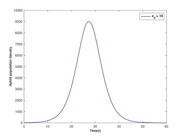
Here h(t)𝑡h(t) is the cumulative population density of a single aphid biotype at time t; x(t)𝑥𝑡x(t) is the population density at time t𝑡t, a𝑎a is a scalar constant, and r𝑟r is the growth rate of the aphids. The aphid population initially rises driven by the linear growth term - this is the “boom” phase, but as the cumulative density becomes greater than the growth rate r𝑟r, the population decreases driven by competition. This results in the “bust” phase [21] and ”boom-bust” phases can be seen in fig 1. This is commonly seen in the population dynamics of aphids and has been observed in soybean aphids in North America [20], with colonization in June, then a gradual buildup of population, peaking in August, and declining with aphids dispersing in September to their overwintering host. These dynamics differ from those predicted by the classical logistic growth model, which shows convergence to the carrying capacity state. This also provides a framework to investigate additional situations such as if the carrying capacity was variable in time.
Refer to caption
Figure 1: The time series figure shows the boom-bust scenario for the Kindlmann Classical Model. The parameter set used: a=0.000005,r=0.3formulae-sequence𝑎0.000005𝑟0.3a=0.000005,r=0.3. The initial aphid population density is inset.

2.2 Logistic Population Model with Variable Carrying Capacity

It has been observed in the field on occasion that the classical (one-peak) boom-bust dynamics will not occur, rather one may see multiple peaks during the growing season, one initially followed by a downturn and then another peak [9]. This could be for a plethora of reasons. Host plant suitability changes over the growing season, environmental and/or weather-driven changes, an excessive abundance of aphids at the beginning of the season, enhanced competition and reduced fecundity [1, 22]. In order to capture such dynamics, the following population model for aphids [1], with variable carrying capacity is introduced. We abbreviate this as VNLM (variable carrying capacity non-local logistic model) henceforth,

dhdt=ax,h(0)=0formulae-sequence𝑑𝑑𝑡𝑎𝑥00\frac{dh}{dt}=ax,\ h(0)=0 (2.3)
dxdt=(rh)x(1xk),x(0)=x0formulae-sequence𝑑𝑥𝑑𝑡𝑟𝑥1𝑥𝑘𝑥0subscript𝑥0\frac{dx}{dt}=(r-h)x\left(1-\frac{x}{k}\right),\ x(0)=x_{0} (2.4)

Here

k=k(t)=(kmaxkmin)f(t)+kmin,f(t)=(cos(dπt)+12)formulae-sequence𝑘𝑘𝑡subscript𝑘𝑚𝑎𝑥subscript𝑘𝑚𝑖𝑛𝑓𝑡subscript𝑘𝑚𝑖𝑛𝑓𝑡𝑐𝑜𝑠𝑑𝜋𝑡12k=k(t)=\left(k_{max}-k_{min}\right)f(t)+k_{min},\ f(t)=\left(\frac{cos(d\pi t)+1}{2}\right) (2.5)

f(t)𝑓𝑡f(t) is modeled as a trigonometric function to mimic the environment/resources fluctuating, such that the total carrying capacity fluctuates between kmaxsubscript𝑘𝑚𝑎𝑥k_{max} and kminsubscript𝑘𝑚𝑖𝑛k_{min} values (as f(t)𝑓𝑡f(t) fluctuates between 00 and 111).

Refer to caption
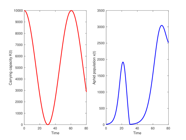
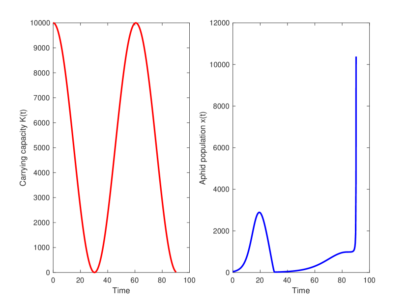
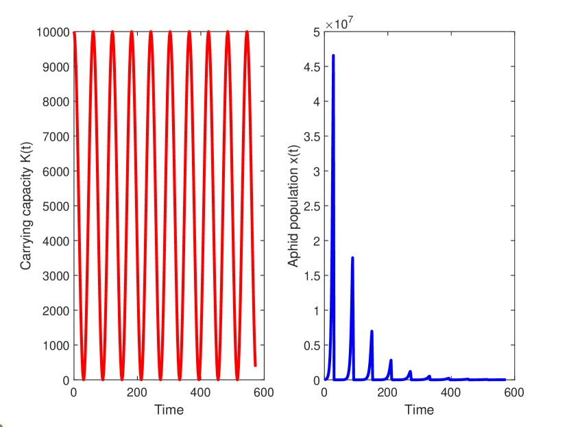
Figure 2: The time series figure shows the carrying capacity and aphid population density with t=80𝑡80t=80 for the Logistic population model with variable carrying capacity. The parameter set used: Kmax=10000,Kmin=1,d=.033,a=0.000005,r=0.3formulae-sequencesubscript𝐾𝑚𝑎𝑥10000formulae-sequencesubscript𝐾𝑚𝑖𝑛1formulae-sequence𝑑.033formulae-sequence𝑎0.000005𝑟0.3K_{max}=10000,K_{min}=1,d=.033,a=0.000005,r=0.3. The initial aphid population density x0=10subscript𝑥010x_{0}=10.
Refer to caption
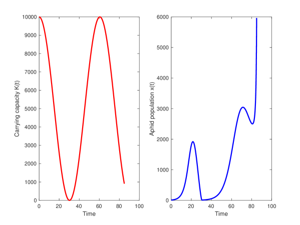
Figure 3: The time series figure shows the carrying capacity and finite time blow-up of the aphid population density at t85𝑡85t\approx 85 for the Logistic population model with variable carrying capacity. The parameter set used: Kmax=10000,Kmin=1,d=.033,a=0.000005,r=0.3formulae-sequencesubscript𝐾𝑚𝑎𝑥10000formulae-sequencesubscript𝐾𝑚𝑖𝑛1formulae-sequence𝑑.033formulae-sequence𝑎0.000005𝑟0.3K_{max}=10000,K_{min}=1,d=.033,a=0.000005,r=0.3. The initial aphid population density x0=10subscript𝑥010x_{0}=10.
Remark 1.

We see via Fig. 2 that the VNLM can predict multiple peaks in a single season, one early on around day 20, and one later at around day 75 - however running the simulation a little longer yields an “exploding” solution around day 85, as seen via Fig. 3.

Thus, the simulation results, as seen via Fig. 3, motivate us to rigorously investigate both analytically and numerically the blow-up dynamic present in the VNLM (2.3)-(2.4).

Remark 2.

Heuristically, the blow-up in the VNLM (2.3)-(2.4) happens when the cumulative density hh exceeds r, and the sign of (rh)𝑟(r-h) is negative. Thus, the standard logistic equation (or even logistic equation with variable carrying capacity k𝑘k) typically described via xx2k𝑥superscript𝑥2𝑘x-\frac{x^{2}}{k}, flips the sign to have a term like x2kxsuperscript𝑥2𝑘𝑥\frac{x^{2}}{k}-x, which can blow-up for sufficiently chosen initial conditions. Similar blow-up results due to sign-changing non-linearity can be seen in works [6, 7].

2.2.1 Some Standard and Auxiliary Results

We state the following lemma,

Lemma 1.

Consider the VNLM given by (2.3)-(2.4). Then for positive initial data x0>0subscript𝑥00x_{0}>0, solutions to (2.3)-(2.4) remain non-negative.

Proof.

The result follows by checking the quasi-positivity condition via Lemma 5. ∎

We present an auxiliary lemma,

Lemma 2.

Consider the VNLM given by (2.3)-(2.4). Then ϵ>0for-allitalic-ϵ0\forall\epsilon>0, δ(ϵ)>0,x0(ϵ)>0formulae-sequence𝛿italic-ϵ0subscriptsuperscript𝑥0italic-ϵ0\exists\delta(\epsilon)>0,x^{*}_{0}(\epsilon)>0 s.t.

x(t)>kmax(rakmin+1)+ϵ,t[0,δ],formulae-sequence𝑥𝑡subscript𝑘𝑚𝑎𝑥𝑟𝑎subscript𝑘𝑚𝑖𝑛1italic-ϵfor-all𝑡0𝛿x(t)>k_{max}\left(\frac{r}{ak_{min}}+1\right)+\epsilon,\ \forall t\in[0,\delta], (2.6)

for all solutions to (2.3)-(2.4), initiating from the initial data x0(ϵ)>0subscriptsuperscript𝑥0italic-ϵ0x^{*}_{0}(\epsilon)>0.

Proof.

The result follows via continuity of solutions to (2.3)-(2.4) via Theorem 4. ∎

2.2.2 Blow-up in finite time in VNLM

We state the following theorem,

Theorem 1.

Consider the VNLM given by (2.3)-(2.4). Then for initial data sufficiently large, solutions to (2.3)-(2.4) blow-up in finite time, that is,

lim suptT<|x(t)|+.subscriptlimit-supremum𝑡superscript𝑇𝑥𝑡\limsup_{t\rightarrow T^{*}<\infty}|x(t)|\rightarrow+\infty. (2.7)
Proof.

Notice,

h(t)=0tax(s)ds=a0tx(s)dsax(t)=>1ah(t)x(t).h(t)=\int^{t}_{0}ax(s)ds=a\int^{t}_{0}x(s)ds\geq ax(t)=>\frac{1}{a}h(t)\geq x(t). (2.8)

We make the following lower estimate,

dxdt𝑑𝑥𝑑𝑡\displaystyle\frac{dx}{dt}
=\displaystyle= (rh)x(1xk)𝑟𝑥1𝑥𝑘\displaystyle(r-h)x\left(1-\frac{x}{k}\right)
=\displaystyle= rxrkx2hx+1khx2𝑟𝑥𝑟𝑘superscript𝑥2𝑥1𝑘superscript𝑥2\displaystyle rx-\frac{r}{k}x^{2}-hx+\frac{1}{k}hx^{2}
\displaystyle\geq rxrkminx2hx+1kmaxhx2𝑟𝑥𝑟subscript𝑘𝑚𝑖𝑛superscript𝑥2𝑥1subscript𝑘𝑚𝑎𝑥superscript𝑥2\displaystyle rx-\frac{r}{k_{min}}x^{2}-hx+\frac{1}{k_{max}}hx^{2}
\displaystyle\geq rxrkminahxhx+1kmaxhx2𝑟𝑥𝑟subscript𝑘𝑚𝑖𝑛𝑎𝑥𝑥1subscript𝑘𝑚𝑎𝑥superscript𝑥2\displaystyle rx-\frac{r}{k_{min}a}hx-hx+\frac{1}{k_{max}}hx^{2}
=\displaystyle= rx(rakmin+1)hx+1kmaxhx2𝑟𝑥𝑟𝑎subscript𝑘𝑚𝑖𝑛1𝑥1subscript𝑘𝑚𝑎𝑥superscript𝑥2\displaystyle rx-\left(\frac{r}{ak_{min}}+1\right)hx+\frac{1}{k_{max}}hx^{2}
=\displaystyle= rx(rakmin+1)(0tax(s)𝑑s)x+1kmaxhx2𝑟𝑥𝑟𝑎subscript𝑘𝑚𝑖𝑛1subscriptsuperscript𝑡0𝑎𝑥𝑠differential-d𝑠𝑥1subscript𝑘𝑚𝑎𝑥superscript𝑥2\displaystyle rx-\left(\frac{r}{ak_{min}}+1\right)\left(\int^{t}_{0}ax(s)ds\right)x+\frac{1}{k_{max}}hx^{2}

Now we proceed by contradiction. Assume x(t)𝑥𝑡x(t) remains bounded on any time interval [0,T],T<0𝑇𝑇[0,T],\ T<\infty, then via the embedding, L(0,T)L1(0,T)superscript𝐿0𝑇superscript𝐿10𝑇L^{\infty}(0,T)\hookrightarrow L^{1}(0,T), we must have that,

0Tax(s)dsTC|||x(t)||.\int^{T}_{0}ax(s)ds\leq TC|||x(t)||_{\infty}. (2.10)

Thus inserting this in the above inequality, which must hold for any t[0,T]𝑡0𝑇t\in[0,T] we have,

dxdt𝑑𝑥𝑑𝑡\displaystyle\frac{dx}{dt} (2.11)
\displaystyle\geq rx(rakmin+1)(0tax(s)𝑑s)x+1kmaxhx2𝑟𝑥𝑟𝑎subscript𝑘𝑚𝑖𝑛1subscriptsuperscript𝑡0𝑎𝑥𝑠differential-d𝑠𝑥1subscript𝑘𝑚𝑎𝑥superscript𝑥2\displaystyle rx-\left(\frac{r}{ak_{min}}+1\right)\left(\int^{t}_{0}ax(s)ds\right)x+\frac{1}{k_{max}}hx^{2}
\displaystyle\geq rx(rakmin+1)(TC|||x(t)||)x+1kmaxax3\displaystyle rx-\left(\frac{r}{ak_{min}}+1\right)\left(TC|||x(t)||_{\infty}\right)x+\frac{1}{k_{max}}ax^{3}
\displaystyle\geq (rM)x+1kmaxax3𝑟𝑀𝑥1subscript𝑘𝑚𝑎𝑥𝑎superscript𝑥3\displaystyle(r-M)x+\frac{1}{k_{max}}ax^{3}

Where TC|||x(t)||<MTC|||x(t)||_{\infty}<M. However, in this case x𝑥x blows up in comparison with the ODE y=C3y3+C4ysuperscript𝑦subscript𝐶3superscript𝑦3subscript𝐶4𝑦\boxed{y^{{}^{\prime}}=C_{3}y^{3}+C_{4}y}, with C4>0subscript𝐶40C_{4}>0 or C4<0subscript𝐶40C_{4}<0. This is a contradiction to x𝑥x being bounded at any T<𝑇T<\infty. Thus x𝑥x must blow up at a finite time T[0,T]superscript𝑇0𝑇T^{*}\in[0,T]. ∎

We next state the following theorem,

Theorem 2.

Consider the VNLM given by (2.3)-(2.4). Then for initial data sufficiently large, that is x0>kmax(rakmin+1)subscript𝑥0subscript𝑘𝑚𝑎𝑥𝑟𝑎subscript𝑘𝑚𝑖𝑛1x_{0}>k_{max}\left(\frac{r}{ak_{min}}+1\right), solutions to (2.3)-(2.4) blow-up in finite time, that is,

lim suptT<|x(t)|+.subscriptlimit-supremum𝑡superscript𝑇𝑥𝑡\limsup_{t\rightarrow T^{*}<\infty}|x(t)|\rightarrow+\infty. (2.12)
Proof.

Using the lower estimate from theorem 1,

dxdtrx(rakmin+1)hx+1kmaxhx2((xkmax)(rakmin+1))hx𝑑𝑥𝑑𝑡𝑟𝑥𝑟𝑎subscript𝑘𝑚𝑖𝑛1𝑥1subscript𝑘𝑚𝑎𝑥superscript𝑥2𝑥subscript𝑘𝑚𝑎𝑥𝑟𝑎subscript𝑘𝑚𝑖𝑛1𝑥\frac{dx}{dt}\geq rx-\left(\frac{r}{ak_{min}}+1\right)hx+\frac{1}{k_{max}}hx^{2}\geq\left(\left(\frac{x}{k_{max}}\right)-\left(\frac{r}{ak_{min}}+1\right)\right)hx (2.13)

Thus x𝑥x blows up trivially for sufficiently large data chosen as per the requirement of lemma 2, in comparison with the ODE, y=ϵy2superscript𝑦italic-ϵsuperscript𝑦2\boxed{y^{{}^{\prime}}=\epsilon y^{2}}, ϵ>0italic-ϵ0\epsilon>0. ∎

Remark 1.

The blow-up in h(t)𝑡h(t), follows using (2.8). In the more general case, one can compare to the ODE, y=C3ypC4yq,p>q>1,C3>0,C4>0formulae-sequencesuperscript𝑦subscript𝐶3superscript𝑦𝑝subscript𝐶4superscript𝑦𝑞𝑝𝑞1formulae-sequencesubscript𝐶30subscript𝐶40\boxed{y^{{}^{\prime}}=C_{3}y^{p}-C_{4}y^{q}},p>q>1,C_{3}>0,C_{4}>0.

Lemma 3.

Consider the VNLM given by (2.3)-(2.4). Then for initial data sufficiently large, that is x0>kmax(rakmin+1)subscript𝑥0subscript𝑘𝑚𝑎𝑥𝑟𝑎subscript𝑘𝑚𝑖𝑛1x_{0}>k_{max}\left(\frac{r}{ak_{min}}+1\right), the cumulative pest density blow-up in finite time, that is,

lim suptT<|h(t)|+.subscriptlimit-supremum𝑡superscript𝑇𝑡\ \limsup_{t\rightarrow T^{*}<\infty}|h(t)|\rightarrow+\infty. (2.14)
Proof.

We know from the mean value theorem of integrals,

1T0Tx(s)𝑑s=x(T),T<,T[0,T].formulae-sequence1𝑇subscriptsuperscript𝑇0𝑥𝑠differential-d𝑠𝑥superscript𝑇absentformulae-sequence𝑇superscript𝑇absent0𝑇\frac{1}{T}\int^{T}_{0}x(s)ds=x(T^{**}),\ T<\infty,\ T^{**}\in[0,T]. (2.15)

Via Theorem 2, we have the blow-up of x(t)𝑥𝑡x(t) at some T<superscript𝑇T^{*}<\infty. Consider,

12(TΔt)x(T)1(TΔt)0TΔtx(s)𝑑s=x(T),12superscript𝑇Δ𝑡𝑥superscript𝑇absent1superscript𝑇Δ𝑡subscriptsuperscriptsuperscript𝑇Δ𝑡0𝑥𝑠differential-d𝑠𝑥superscript𝑇absent\frac{1}{2(T^{*}-\Delta t)}x(T^{**})\leq\frac{1}{(T^{*}-\Delta t)}\int^{T^{*}-\Delta t}_{0}x(s)ds=x(T^{**}), (2.16)

Now taking the limit as Δt0Δ𝑡0\Delta t\rightarrow 0 entails, TTsuperscript𝑇absentsuperscript𝑇T^{**}\rightarrow T^{*}, thus we have

12(T)x(T)=1T0Tx(s)𝑑s=x(T)=,12superscript𝑇𝑥superscript𝑇1superscript𝑇subscriptsuperscriptsuperscript𝑇0𝑥𝑠differential-d𝑠𝑥superscript𝑇\frac{1}{2(T^{*})}x(T^{*})=\infty\leq\frac{1}{T^{*}}\int^{T^{*}}_{0}x(s)ds=x(T^{*})=\infty, (2.17)

The result follows via the squeezing theorem.

2.2.3 Blow-up for other initial conditions

We next explore the case when blow-up is possible for other positive initial data, possibly small.

Remark 2.

The estimate via Theorem 2, is only sufficient, in that if initial data is large enough, x0>kmax(rakmin+1)subscript𝑥0subscript𝑘𝑚𝑎𝑥𝑟𝑎subscript𝑘𝑚𝑖𝑛1x_{0}>k_{max}\left(\frac{r}{ak_{min}}+1\right), then blow-up will occur. This threshold depends strongly on the parameter a𝑎a.

The smaller a𝑎a is the larger the data required for blow-up. However, this is not seen in simulations. Rather small a𝑎a leads to blow-up for essentially any positive initial condition. This motivates proving blow-up for any positive initial data under certain parametric restrictions. One approach is to “construct” a lower solution and derive conditions under which this lower solution blows-up for any initial condition.

An “approximate” ODE for the lower estimate is given by,

dxdt=akmaxx3(rkmin+a)x2+rx𝑑𝑥𝑑𝑡𝑎subscript𝑘𝑚𝑎𝑥superscript𝑥3𝑟subscript𝑘𝑚𝑖𝑛𝑎superscript𝑥2𝑟𝑥\frac{dx}{dt}=\frac{a}{k_{max}}x^{3}-\left(\frac{r}{k_{min}}+a\right)x^{2}+rx (2.18)

We note this is only a crude approximation because (without enforcing any positivity conditions) we require,

h(t)=0tax(s)𝑑sx(t),𝑡subscriptsuperscript𝑡0𝑎𝑥𝑠differential-d𝑠𝑥𝑡h(t)=\int^{t}_{0}ax(s)ds\approx x(t), (2.19)

If one applies this “approximation” and explores the cubic,

(akmax)x3(rkmin+a)x2+rx=x((akmax)x2(rkmin+a)x+r)𝑎subscript𝑘𝑚𝑎𝑥superscript𝑥3𝑟subscript𝑘𝑚𝑖𝑛𝑎superscript𝑥2𝑟𝑥𝑥𝑎subscript𝑘𝑚𝑎𝑥superscript𝑥2𝑟subscript𝑘𝑚𝑖𝑛𝑎𝑥𝑟\left(\frac{a}{k_{max}}\right)x^{3}-\left(\frac{r}{k_{min}}+a\right)x^{2}+rx=x\left(\left(\frac{a}{k_{max}}\right)x^{2}-\left(\frac{r}{k_{min}}+a\right)x+r\right) (2.20)

This has one real zero, x=0𝑥0x=0, for others we check discriminant. Then, the other two roots must be complex. Since the coefficient of the leading term in the cubic is positive, it must approach positive infinity as x𝑥x\rightarrow\infty. Thus, standard phase analysis will yield blow-up for any positive initial data. The required condition for this is,

(rkmin+a)24(akmax)r<0superscript𝑟subscript𝑘𝑚𝑖𝑛𝑎24𝑎subscript𝑘𝑚𝑎𝑥𝑟0\left(\frac{r}{k_{min}}+a\right)^{2}-4\left(\frac{a}{k_{max}}\right)r<0 (2.21)

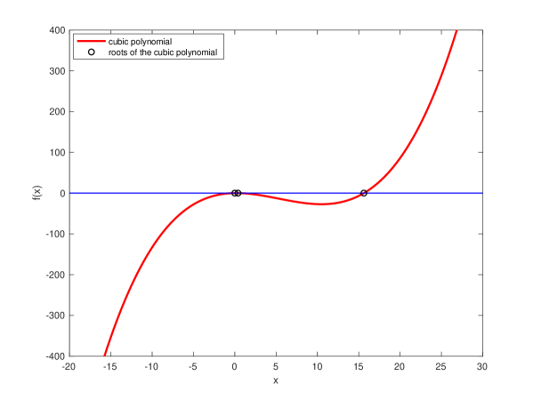
However, this is never true as kmax>kminsubscript𝑘𝑚𝑎𝑥subscript𝑘𝑚𝑖𝑛k_{max}>k_{min}. Thus there exist two positive roots, which yield blow-up in finite time for the cubic ODE (2.20)
Refer to caption
Figure 4: This figure represents the cubic polynomial in (2.20). The parameter set used: Kmax=10,Kmin=1,a=0.5,r=0.3formulae-sequencesubscript𝐾𝑚𝑎𝑥10formulae-sequencesubscript𝐾𝑚𝑖𝑛1formulae-sequence𝑎0.5𝑟0.3K_{max}=10,K_{min}=1,a=0.5,r=0.3.

2.2.4 Blow-up via delay equations

We recap the following result from the literature, [23]

Proposition 1.

Consider the following delayed equation

y(t)=|y(t)|p|y(tτ)|q,t>0,formulae-sequencesuperscript𝑦𝑡superscript𝑦𝑡𝑝superscript𝑦𝑡𝜏𝑞𝑡0\displaystyle y^{{}^{\prime}}(t)=|y(t)|^{p}-|y(t-\tau)|^{q},\ t>0,
y(τ1)=ϕ(τ1),τ1[τ,0].formulae-sequence𝑦subscript𝜏1italic-ϕsubscript𝜏1subscript𝜏1𝜏0\displaystyle y(\tau_{1})=\phi(\tau_{1}),\ \tau_{1}\in[-\tau,0].

Assume that p>max(q,1)𝑝𝑞1p>\max{(q,1)} and ϕitalic-ϕ\phi satisfying ϕ(0)|ϕ(t)|qpitalic-ϕ0superscriptitalic-ϕ𝑡𝑞𝑝\phi(0)\geq|\phi(t)|^{\frac{q}{p}} for all t[τ,0],ϕ(0)1,ϕ(0)>|ϕ(τ)|qpformulae-sequence𝑡𝜏0formulae-sequenceitalic-ϕ01italic-ϕ0superscriptitalic-ϕ𝜏𝑞𝑝t\in[-\tau,0],\phi(0)\geq 1,\phi(0)>|\phi(-\tau)|^{\frac{q}{p}}, then the solution (1) blows-up in finite time.

In order to proceed, we need to modify the above and state the following Theorem,

Theorem 2.1.

Consider the following delayed equation

y(t)=|y(t)|pM|y(tτ)|q,t>0,formulae-sequencesuperscript𝑦𝑡superscript𝑦𝑡𝑝𝑀superscript𝑦𝑡𝜏𝑞𝑡0\displaystyle y^{{}^{\prime}}(t)=|y(t)|^{p}-M|y(t-\tau)|^{q},\ t>0,
y(τ1)=ϕ(τ1),τ1[τ,0].formulae-sequence𝑦subscript𝜏1italic-ϕsubscript𝜏1subscript𝜏1𝜏0\displaystyle y(\tau_{1})=\phi(\tau_{1}),\ \tau_{1}\in[-\tau,0].

Assume that p>max(q,1)𝑝𝑞1p>\max{(q,1)} and ϕitalic-ϕ\phi satisfying ϕ(0)M1p|ϕ(t)|qpitalic-ϕ0superscript𝑀1𝑝superscriptitalic-ϕ𝑡𝑞𝑝\phi(0)\geq M^{\frac{1}{p}}|\phi(t)|^{\frac{q}{p}} for all t[τ,0],ϕ(0)M,ϕ(0)>M1p|ϕ(τ)|qpformulae-sequence𝑡𝜏0formulae-sequenceitalic-ϕ0𝑀italic-ϕ0superscript𝑀1𝑝superscriptitalic-ϕ𝜏𝑞𝑝t\in[-\tau,0],\phi(0)\geq M,\phi(0)>M^{\frac{1}{p}}|\phi(-\tau)|^{\frac{q}{p}}, then the solution (2.1) blows-up in finite time.

The proof follows ideas in [23].

Proof.

Assume that there is a maximal time of existence Tsuperscript𝑇T^{*} to the solution of (2.1). Via the equation, y>0superscript𝑦0y^{{}^{\prime}}>0, thus y𝑦y is increasing. Let

t1=sup{t0,y(s)>0,s[0,t]}.subscript𝑡1supremumformulae-sequence𝑡0formulae-sequencesuperscript𝑦𝑠0𝑠0𝑡t_{1}=\sup\{t\geq 0,y^{{}^{\prime}}(s)>0,s\in[0,t]\}. (2.24)

If t1<Tsubscript𝑡1superscript𝑇t_{1}<T^{*}, then y(t1)=0superscript𝑦subscript𝑡10y^{{}^{\prime}}(t_{1})=0. Now let us consider 2 cases.

Case I: t1<τsubscript𝑡1𝜏t_{1}<\tau

Since y(t1)=0superscript𝑦subscript𝑡10y^{{}^{\prime}}(t_{1})=0, we have

|y(t1)|pM|ϕ(t1τ)|q=0.superscript𝑦subscript𝑡1𝑝𝑀superscriptitalic-ϕsubscript𝑡1𝜏𝑞0|y(t_{1})|^{p}-M|\phi(t_{1}-\tau)|^{q}=0. (2.25)

This is not possible due to the increasing dynamic of y𝑦y,

|y(t1)|p>|y(0)|p=|ϕ(0)|pM|ϕ(t1τ)|q.superscript𝑦subscript𝑡1𝑝superscript𝑦0𝑝superscriptitalic-ϕ0𝑝𝑀superscriptitalic-ϕsubscript𝑡1𝜏𝑞|y(t_{1})|^{p}>|y(0)|^{p}=|\phi(0)|^{p}\geq M|\phi(t_{1}-\tau)|^{q}. (2.26)

Case II: t1>τsubscript𝑡1𝜏t_{1}>\tau

In this case, again since y(t1)=0superscript𝑦subscript𝑡10y^{{}^{\prime}}(t_{1})=0, we have

|y(t1)|pM|y(t1τ)|q=0.superscript𝑦subscript𝑡1𝑝𝑀superscript𝑦subscript𝑡1𝜏𝑞0|y(t_{1})|^{p}-M|y(t_{1}-\tau)|^{q}=0. (2.27)

Now y(t)>y(0)=ϕ(0)M1𝑦𝑡𝑦0italic-ϕ0𝑀1y(t)>y(0)=\phi(0)\geq M\geq 1.

so

|y(t1)|=M1p|y(t1τ)|qp<M1p|y(t1τ)|.𝑦subscript𝑡1superscript𝑀1𝑝superscript𝑦subscript𝑡1𝜏𝑞𝑝superscript𝑀1𝑝𝑦subscript𝑡1𝜏|y(t_{1})|=M^{\frac{1}{p}}|y(t_{1}-\tau)|^{\frac{q}{p}}<M^{\frac{1}{p}}|y(t_{1}-\tau)|. (2.28)

On the other hand

|y(t1)|p>|y(t1τ2)|p.superscript𝑦subscript𝑡1𝑝superscript𝑦subscript𝑡1𝜏2𝑝|y(t_{1})|^{p}>|y\left(t_{1}-\frac{\tau}{2}\right)|^{p}. (2.29)

Thus we have

|y(t1τ2)|pM|y(t1τ)|q<0,superscript𝑦subscript𝑡1𝜏2𝑝𝑀superscript𝑦subscript𝑡1𝜏𝑞0|y\left(t_{1}-\frac{\tau}{2}\right)|^{p}-M|y(t_{1}-\tau)|^{q}<0, (2.30)

but this would imply y(t)=0superscript𝑦𝑡0y^{{}^{\prime}}(t)=0, at some t<t1τ2𝑡subscript𝑡1𝜏2t<t_{1}-\frac{\tau}{2}, contradicting the fact that t1subscript𝑡1t_{1} is the supremum of the earlier set constructed in (2.24). This entails that, y𝑦y is increasing on [0,T)0superscript𝑇[0,T^{*}). Thus y(t)pMy(tτ)q>0𝑦superscript𝑡𝑝𝑀𝑦superscript𝑡𝜏𝑞0y(t)^{p}-My(t-\tau)^{q}>0, and thus so is y(t)qMy(tτ)q>0𝑦superscript𝑡𝑞𝑀𝑦superscript𝑡𝜏𝑞0y(t)^{q}-My(t-\tau)^{q}>0. Hence rearranging (2.1), we have,

y(t)=y(t)py(t)q+(y(t)qMy(tτ)q)superscript𝑦𝑡𝑦superscript𝑡𝑝𝑦superscript𝑡𝑞𝑦superscript𝑡𝑞𝑀𝑦superscript𝑡𝜏𝑞y^{{}^{\prime}}(t)=y(t)^{p}-y(t)^{q}+\left(y(t)^{q}-My(t-\tau)^{q}\right) (2.31)

Using the positivity results derived earlier, blow-up at a finite time Tsuperscript𝑇T^{*}, for sufficiently large data is immediate in comparison with an ODE of the form y(t)=y(t)py(t)qsuperscript𝑦𝑡𝑦superscript𝑡𝑝𝑦superscript𝑡𝑞y^{{}^{\prime}}(t)=y(t)^{p}-y(t)^{q}. This proves the theorem.

Now we can state the following theorem,

Theorem 3.

Consider the VNLM given by (2.3)-(2.4). Then for initial data sufficiently large, that is x0>kmax(rakmin+1)kmax(rakmin+1)T2a2subscript𝑥0subscript𝑘𝑚𝑎𝑥𝑟𝑎subscript𝑘𝑚𝑖𝑛1subscript𝑘𝑚𝑎𝑥𝑟𝑎subscript𝑘𝑚𝑖𝑛1superscript𝑇2superscript𝑎2x_{0}>k_{max}\left(\frac{r}{ak_{min}}+1\right)k_{max}\left(\frac{r}{ak_{min}}+1\right)\frac{T^{2}}{a^{2}}, solutions to (2.3)-(2.4) blow-up in finite time, that is,

lim suptT<|x(t)|+.subscriptlimit-supremum𝑡superscript𝑇𝑥𝑡\limsup_{t\rightarrow T^{*}<\infty}|x(t)|\rightarrow+\infty. (2.32)
Proof.

We begin with the following estimate on a time interval t[0,T],T<formulae-sequence𝑡0𝑇𝑇t\in[0,T],T<\infty.

dxdt𝑑𝑥𝑑𝑡\displaystyle\frac{dx}{dt} (2.33)
\displaystyle\geq rx(rakmin+1)hx+1kmaxhx2𝑟𝑥𝑟𝑎subscript𝑘𝑚𝑖𝑛1𝑥1subscript𝑘𝑚𝑎𝑥superscript𝑥2\displaystyle rx-\left(\frac{r}{ak_{min}}+1\right)hx+\frac{1}{k_{max}}hx^{2}
\displaystyle\geq rx(rakmin+1)1ah2+1kmaxhx2𝑟𝑥𝑟𝑎subscript𝑘𝑚𝑖𝑛11𝑎superscript21subscript𝑘𝑚𝑎𝑥superscript𝑥2\displaystyle rx-\left(\frac{r}{ak_{min}}+1\right)\frac{1}{a}h^{2}+\frac{1}{k_{max}}hx^{2}
=\displaystyle= rx(rakmin+1)1a(0tx(s)𝑑s)2+1kmaxhx2𝑟𝑥𝑟𝑎subscript𝑘𝑚𝑖𝑛11𝑎superscriptsubscriptsuperscript𝑡0𝑥𝑠differential-d𝑠21subscript𝑘𝑚𝑎𝑥superscript𝑥2\displaystyle rx-\left(\frac{r}{ak_{min}}+1\right)\frac{1}{a}\left(\int^{t}_{0}x(s)ds\right)^{2}+\frac{1}{k_{max}}hx^{2}
=\displaystyle= rx(rakmin+1)T2a(x(tτ))2+1kmaxax3𝑟𝑥𝑟𝑎subscript𝑘𝑚𝑖𝑛1superscript𝑇2𝑎superscript𝑥𝑡𝜏21subscript𝑘𝑚𝑎𝑥𝑎superscript𝑥3\displaystyle rx-\left(\frac{r}{ak_{min}}+1\right)\frac{T^{2}}{a}\left(x(t-\tau)\right)^{2}+\frac{1}{k_{max}}ax^{3}
\displaystyle\geq 1kmaxax3(rakmin+1)T2a(x(tτ))21subscript𝑘𝑚𝑎𝑥𝑎superscript𝑥3𝑟𝑎subscript𝑘𝑚𝑖𝑛1superscript𝑇2𝑎superscript𝑥𝑡𝜏2\displaystyle\frac{1}{k_{max}}ax^{3}-\left(\frac{r}{ak_{min}}+1\right)\frac{T^{2}}{a}\left(x(t-\tau)\right)^{2}

Now, if we choose initial data s.t.

x0>kmax(rakmin+1)T2a2subscript𝑥0subscript𝑘𝑚𝑎𝑥𝑟𝑎subscript𝑘𝑚𝑖𝑛1superscript𝑇2superscript𝑎2x_{0}>k_{max}\left(\frac{r}{ak_{min}}+1\right)\frac{T^{2}}{a^{2}} (2.34)

Then a direct application of Theorem 2.1 yields the finite time blow-up of x𝑥x.

2.3 An Alternate Model

We next propose an alternate model, taking our cue from the model proposed in [1]. Here we suppose that the cumulative density at time level t𝑡t depends on the cumulative population at time tτ1𝑡subscript𝜏1t-\tau_{1}, for suitably chosen τ1subscript𝜏1\tau_{1}. The logistic term is also replaced by the classic delayed logistic term. Delayed differential equations have a rich variety of applications in population biology models, see [24] for more details. We consider the following model,

dhdt=ax(tτ1),τ1>0,h(0)=0.formulae-sequence𝑑𝑑𝑡𝑎𝑥𝑡subscript𝜏1formulae-sequencesubscript𝜏1000\frac{dh}{dt}=ax(t-\tau_{1}),\ \tau_{1}>0,\ h(0)=0. (2.35)
dxdt=(rh)x(1x(tτ2)k),τ2>0.formulae-sequence𝑑𝑥𝑑𝑡𝑟𝑥1𝑥𝑡subscript𝜏2𝑘subscript𝜏20\frac{dx}{dt}=(r-h)x\left(1-\frac{x(t-\tau_{2})}{k}\right),\ \tau_{2}>0. (2.36)

subject to initial conditions

x(θ)=ϕ1(θ)>0,θ[τ,0);ϕ1(0)>0,formulae-sequence𝑥𝜃subscriptitalic-ϕ1𝜃0formulae-sequence𝜃𝜏0subscriptitalic-ϕ100x(\theta)=\phi_{1}(\theta)>0,\theta\in[-\tau,0);\quad\phi_{1}(0)>0, (2.37)

2.4 Local Boundedness

We state the following Lemma,

Lemma 2.2.

Consider the delayed model (2.35)-(2.37). Given an initial condition, arbitrarily large, there exist choices of the delay parameters τ1,τ2subscript𝜏1subscript𝜏2\tau_{1},\tau_{2} s.t. the solutions to (2.35)-(2.37) exist for all time.

Proof.

Via simple comparison, we have

dxdthxx(tτ2)kTax(tτ3)xx(tτ2)k𝑑𝑥𝑑𝑡𝑥𝑥𝑡subscript𝜏2𝑘𝑇𝑎𝑥𝑡subscript𝜏3𝑥𝑥𝑡subscript𝜏2𝑘\frac{dx}{dt}\leq hx\frac{x(t-\tau_{2})}{k}\leq Tax(t-\tau_{3})x\frac{x(t-\tau_{2})}{k} (2.38)

This follows via the mean value theorem for integrals,

h(t)=0tax(sτ1)𝑑s=Tax(tτ3),τ3>τ1,t[0,T].formulae-sequence𝑡subscriptsuperscript𝑡0𝑎𝑥𝑠subscript𝜏1differential-d𝑠𝑇𝑎𝑥𝑡subscript𝜏3formulae-sequencesubscript𝜏3subscript𝜏1𝑡0𝑇h(t)=\int^{t}_{0}ax(s-\tau_{1})ds=Tax(t-\tau_{3}),\ \tau_{3}>\tau_{1},\ t\in[0,T]. (2.39)

here WLOG we assume τ2>τ3subscript𝜏2subscript𝜏3\tau_{2}>\tau_{3}. Now we proceed via contradiction. Let us assume x𝑥x is not bounded for all time and in fact, blows up at a finite time T<superscript𝑇T^{*}<\infty. Then we can divide the inequality (2.38) by x𝑥x, and integrate in the time interval [0,T]0superscript𝑇[0,T^{*}] to obtain,

ln(x(T))ln(x(0))=Takmin0Tx(tτ3)x(tτ2)𝑑tTakminsupt[0,T]|x(tτ3)|0Tx(tτ2)𝑑t<.𝑥superscript𝑇𝑥0superscript𝑇𝑎subscript𝑘𝑚𝑖𝑛subscriptsuperscriptsuperscript𝑇0𝑥𝑡subscript𝜏3𝑥𝑡subscript𝜏2differential-d𝑡superscript𝑇𝑎subscript𝑘𝑚𝑖𝑛subscriptsupremum𝑡0superscript𝑇𝑥𝑡subscript𝜏3subscriptsuperscriptsuperscript𝑇0𝑥𝑡subscript𝜏2differential-d𝑡\ln(x(T^{*}))-\ln(x(0))=\infty\leq\frac{T^{*}a}{k_{min}}\int^{T^{*}}_{0}x(t-\tau_{3})x(t-\tau_{2})dt\leq\frac{T^{*}a}{k_{min}}\sup_{t\in[0,T^{*}]}|x(t-\tau_{3})|\int^{T^{*}}_{0}x(t-\tau_{2})dt<\infty. (2.40)

This follows as we assume x𝑥x only blows up at time t=T𝑡superscript𝑇t=T^{*}, and so must be bounded at all earlier times, thus

supt[0,T]|x(tτ3)|<.subscriptsupremum𝑡0superscript𝑇𝑥𝑡subscript𝜏3\sup_{t\in[0,T^{*}]}|x(t-\tau_{3})|<\infty. (2.41)

Furthermore,

0Tx(tτ2)𝑑s0Tτ2x(s)𝑑s+ϕ1(s)τ2<.subscriptsuperscriptsuperscript𝑇0𝑥𝑡subscript𝜏2differential-d𝑠subscriptsuperscriptsuperscript𝑇subscript𝜏20𝑥𝑠differential-d𝑠subscriptitalic-ϕ1𝑠subscript𝜏2\int^{T^{*}}_{0}x(t-\tau_{2})ds\leq\int^{T^{*}-\tau_{2}}_{0}x(s)ds+\phi_{1}(s)\tau_{2}<\infty. (2.42)

The result follows via simple comparison.

Remark 3.

In the proof above, we require τ2>τ3subscript𝜏2subscript𝜏3\tau_{2}>\tau_{3} in application of the mean value theorem. If this is not achievable given the initial conditions and other parameters, blow-up may not be preventable. Also, for arbitrary initial functions x(θ)=ϕ1(θ)>0,θ[τ,0);ϕ1(0)>0formulae-sequence𝑥𝜃subscriptitalic-ϕ1𝜃0formulae-sequence𝜃𝜏0subscriptitalic-ϕ100x(\theta)=\phi_{1}(\theta)>0,\theta\in[-\tau,0);\quad\phi_{1}(0)>0, and fixed delays τ2,τ1subscript𝜏2subscript𝜏1\tau_{2},\tau_{1}, blow-up may not be preventable - that is one may have a blow-up solution.

3 Numerical Simulations

3.1 Blow-up Dynamics of VNLM Model
Refer to caption
(a)
Refer to caption
(b)
Refer to caption
(c)
Refer to caption
(d)
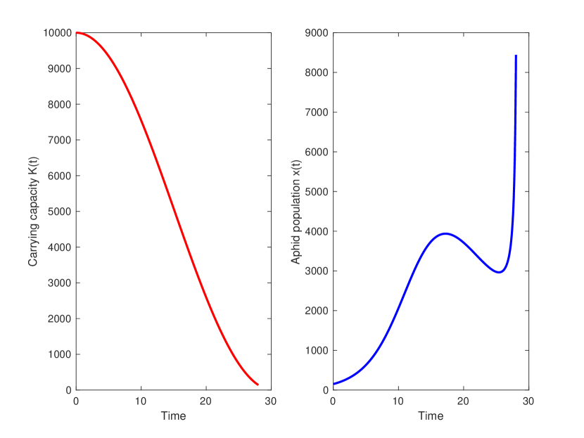
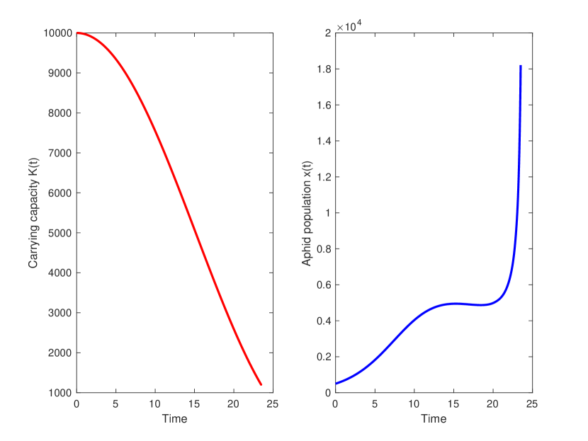
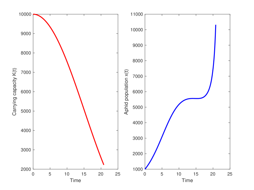
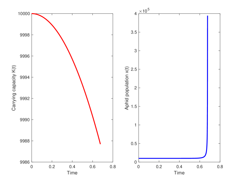
Figure 5: The time series figure shows the carrying capacity and finite time blow-up in aphid population with variation in the initial population. The parameter set: Kmax=10000,Kmin=1,d=.033,a=0.000005,r=0.3formulae-sequencesubscript𝐾𝑚𝑎𝑥10000formulae-sequencesubscript𝐾𝑚𝑖𝑛1formulae-sequence𝑑.033formulae-sequence𝑎0.000005𝑟0.3K_{max}=10000,K_{min}=1,d=.033,a=0.000005,r=0.3. The aphid population blows up at: 5(a)) x0=40subscript𝑥040x_{0}=40, t85𝑡85t\approx 85 with x2000𝑥2000x\approx 2000, 5(b)) x0=150subscript𝑥0150x_{0}=150, t28𝑡28t\approx 28 with x4800𝑥4800x\approx 4800, 5(c)) x0=500subscript𝑥0500x_{0}=500, t23𝑡23t\approx 23 with x6800𝑥6800x\approx 6800 5(d)) x0=1000subscript𝑥01000x_{0}=1000, t21𝑡21t\approx 21 with x7800𝑥7800x\approx 7800.
Blow-up time with variation in ``a"``𝑎"``a"
Value of ``a"``𝑎"``a" Blow-up for initial data x0subscript𝑥0x_{0} Blow-up time (days)
0.000005 105 \approx 30
0.00005 10 \approx 27
0.0005 1 \approx 30
0.005 9999 \approx 1
Refer to caption
(a)
Refer to caption
(b)
Refer to caption
(c)
Refer to caption
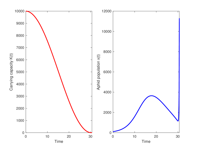
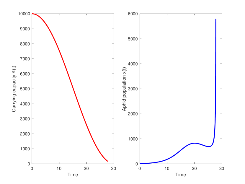
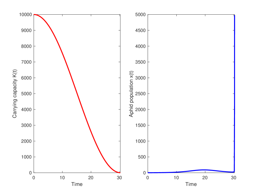
(d)
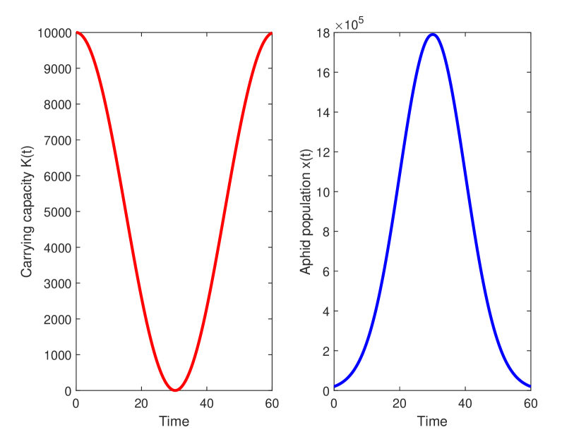
Figure 6: The time series figure shows the carrying capacity and finite time blow-up with variation in ``a"``𝑎"``a". The parameter set: Kmax=10000,Kmin=1,d=.033,r=0.3formulae-sequencesubscript𝐾𝑚𝑎𝑥10000formulae-sequencesubscript𝐾𝑚𝑖𝑛1formulae-sequence𝑑.033𝑟0.3K_{max}=10000,K_{min}=1,d=.033,r=0.3. For 6(a)) a=0.000005𝑎0.000005a=0.000005, x0=105subscript𝑥0105x_{0}=105 and population blows up at t30𝑡30t\approx 30, 6(b)) a=0.00005𝑎0.00005a=0.00005, x0=10subscript𝑥010x_{0}=10 and population blows up at t27𝑡27t\approx 27, 6(c)) a=0.0005𝑎0.0005a=0.0005, x0=1subscript𝑥01x_{0}=1 and population blows up at t30𝑡30t\approx 30 6(d)) a=0.005𝑎0.005a=0.005, x0=9999subscript𝑥09999x_{0}=9999 and population blows up at t1𝑡1t\approx 1.

3.2 Dynamics of the delay model
Refer to caption
(a)
Refer to caption
(b)
Refer to caption
(c)
Refer to caption
(d)
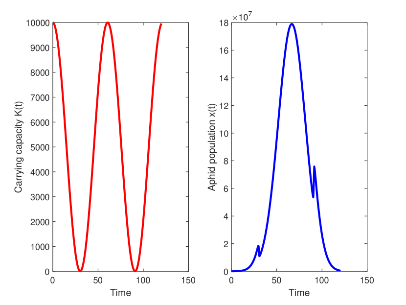
Figure 7: The time series figure shows the carrying capacity and prevention of finite time blow-up with variation in ``a"``𝑎"``a". The parameter set: Kmax=10000,Kmin=1,d=.033,r=0.3formulae-sequencesubscript𝐾𝑚𝑎𝑥10000formulae-sequencesubscript𝐾𝑚𝑖𝑛1formulae-sequence𝑑.033𝑟0.3K_{max}=10000,K_{min}=1,d=.033,r=0.3. The initial population is taken high, i.e., x0=20,000subscript𝑥020000x_{0}=20,000. Different delay parameters (τ1,τ2)subscript𝜏1subscript𝜏2(\tau_{1},\tau_{2}) and parameter a𝑎a has been used. The parameters used are 7(a)) (τ1,τ2)=(2,2)subscript𝜏1subscript𝜏222(\tau_{1},\tau_{2})=(2,2) and a=0.005𝑎0.005a=0.005, 7(b)) (τ1,τ2)=(7,7)subscript𝜏1subscript𝜏277(\tau_{1},\tau_{2})=(7,7) and a=0.0005𝑎0.0005a=0.0005, 7(c)) (τ1,τ2)=(60,60)subscript𝜏1subscript𝜏26060(\tau_{1},\tau_{2})=(60,60) and a=0.00005𝑎0.00005a=0.00005 and 7(d)) (τ1,τ2)=(100,100)subscript𝜏1subscript𝜏2100100(\tau_{1},\tau_{2})=(100,100) and a=0.000005𝑎0.000005a=0.000005.
Refer to caption
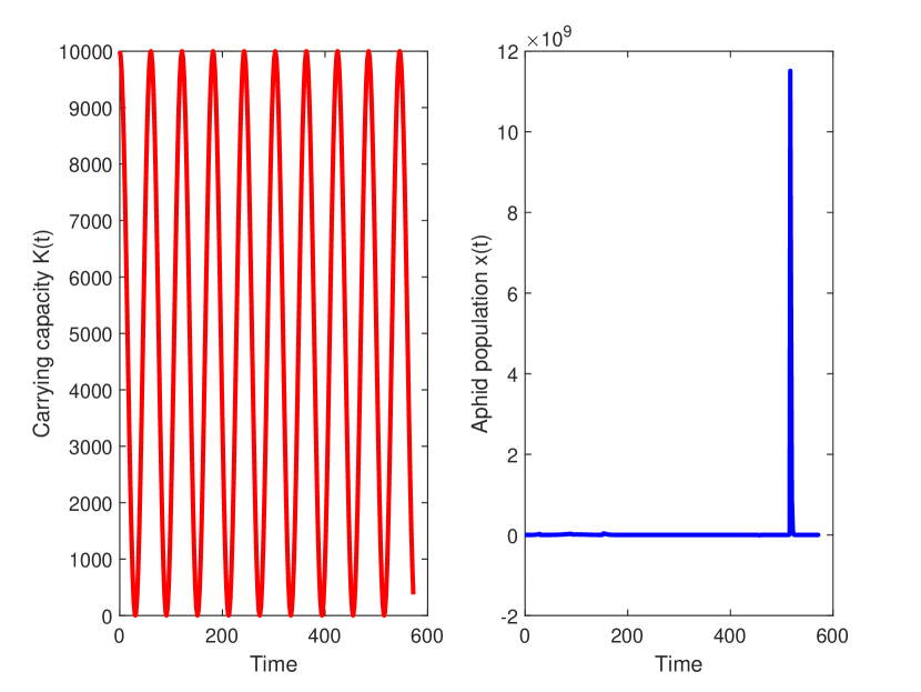
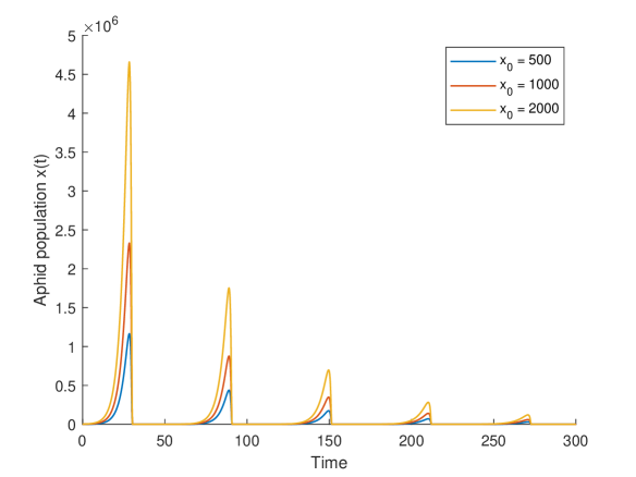
Figure 8: The figure shows times series for different initial population x0subscript𝑥0x_{0} where parameters taken are Kmax=10000,Kmin=1,d=.033,r=0.3,(τ1,τ2)=(100,100)formulae-sequencesubscript𝐾𝑚𝑎𝑥10000formulae-sequencesubscript𝐾𝑚𝑖𝑛1formulae-sequence𝑑.033formulae-sequence𝑟0.3subscript𝜏1subscript𝜏2100100K_{max}=10000,K_{min}=1,d=.033,r=0.3,(\tau_{1},\tau_{2})=(100,100) and a=0.000005𝑎0.000005a=0.000005.

4 Discussion And Conclusion

In the current work, we see that the VNLM proposed in [1] possesses extremely rich dynamics and is capable of predicting multiple population peaks as is observed in the field with many species of aphids (see Fig. 2). However, the model also possesses finite time blow-up solutions (see Fig. 3) that have not been reported earlier in the literature, to the best of our knowledge. We also see introducing delay parameters enables us to mimic many of these multiple peak dynamics while damping the blow-up solutions (see Fig. 8).

In section 3, we analyze the dynamics of blow-up as seen in VNLM given by (2.3)-(2.4) and also analyze the prevention of blow-up by delay model defined by (2.35) - (2.36) using numerical simulations. In figure 5, a fixed parameter set is used to study the time series with different initial aphid populations (x0subscript𝑥0x_{0}). The time series analysis shows with the increase in initial conditions for the fixed parameter set, the blow-up time for the population decreases. So, the starting population of the aphids plays an important role in determining when a blow-up will occur. In figure 6, we analyze the effect of different parameters on the blow-up dynamics of the VNLM and conclude that parameter a𝑎a plays the most efficient part. The summary of the effect of parameter a𝑎a is shown in table 3.1 as well. We have seen a decrease in a𝑎a can change the initial population threshold for which VNLM will have blow-up dynamics. For some values of a𝑎a, a blow-up can be caused for any initial population.

The authors propose a delay model that can help prevent the blow-up scenario in the VNLM. The prevention is studied using numerical simulations of the delay model as seen in figure 7. The parameters of the table 3.1 have been kept constant, and different delay parameter values (τ1,τ2)subscript𝜏1subscript𝜏2(\tau_{1},\tau_{2}) have been used. It can be concluded from the numerical study that for any blow-up scenario in VNLM, there exists a set of (τ1,τ2)subscript𝜏1subscript𝜏2(\tau_{1},\tau_{2}) for which the system remains bounded. In figure 8, it can be analyzed and seen that for different initial values, we can have a bounded solution with multiple peaks, which is the original motivation of the VNLM. Different peaks of an aphid population can be observed over a season, and the proposed delay model can be used to overcome the shortcomings of the VNLM.

As remarked by the authors in [1], the basic construction of the variable carrying capacity function k(t)𝑘𝑡k(t) is not completely resolved. Furthermore, the “trend” of food quality and quantity during a growing season may be difficult to measure. Mathematically, it remains to be resolved what forms of k(t)𝑘𝑡k(t), could possibly prevent “exploding” solutions. One could for example, even consider k(tτ)𝑘𝑡𝜏k(t-\tau) for reasonable τ>0𝜏0\tau>0. Furthermore, from a purely mathematical angle, one can investigate deriving the necessary conditions for finite-time blow-up solutions in the VNLM. We see numerically that the smaller the parameter a𝑎a is, the smaller the data required to produce a finite-time blow-up solution is. This is unproven by us presently and warrants further investigation.

An accurate construction of a biologically sound model, taking into account all of the nuances involved in the relevant Aphid biology, remains a primary objective for future work. To this end, we would like to explore various alternate reasons for a variable carrying capacity. These will include varying host plant suitability or weather events such as floods or drought. In particular, those that happen early in the season and so possibly dictate the carrying capacity to some extent during the season will also be explored. These and related questions are the subject of our current ongoing investigations.

5 Appendix

We discuss some preliminary well-established results that ensure the non-negativity of solutions and establish both local and global existence, as outlined in [8, 5],

Lemma 4.

Let us consider the following m×m𝑚𝑚m\times m - ODE system: for all i=1,,m,𝑖1𝑚i=1,...,m,

dXidt=fi(X1,,Xm)inn×+,Xi(0)=Xi0,formulae-sequence𝑑subscript𝑋𝑖𝑑𝑡subscript𝑓𝑖subscript𝑋1subscript𝑋𝑚𝑖𝑛superscript𝑛subscriptsubscript𝑋𝑖0subscript𝑋𝑖0\frac{dX_{i}}{dt}=f_{i}(X_{1},...,X_{m})~{}in~{}\mathbb{R}^{n}\times\mathbb{R}_{+},\ X_{i}(0)=X_{i0}, (5.1)

where f=(f1,,fm):mm:𝑓subscript𝑓1subscript𝑓𝑚superscript𝑚superscript𝑚f=(f_{1},...,f_{m}):\mathbb{R}^{m}\rightarrow\mathbb{R}^{m} is C1(0,T)superscript𝐶10𝑇C^{1}(0,T) and Xi0L(0,T)subscript𝑋𝑖0superscript𝐿0𝑇X_{i0}\in L^{\infty}(0,T), Tfor-all𝑇\forall T. Then there exists a T>0𝑇0T>0 and a unique classical solution of (5.1) on [0,T).0𝑇[0,T). If Tsuperscript𝑇T^{*} denotes the greatest of these Tssuperscript𝑇𝑠T^{\prime}s, then

[supt[0,T),1imXi(t)L(0,T)<+][T=+].delimited-[]subscriptsupremumformulae-sequence𝑡0superscript𝑇1𝑖𝑚subscriptnormsubscript𝑋𝑖𝑡superscript𝐿0𝑇delimited-[]superscript𝑇\Bigg{[}\sup_{t\in[0,T^{*}),1\leq i\leq m}||X_{i}(t)||_{L^{\infty}(0,T)}<+\infty\Bigg{]}\implies[T^{*}=+\infty].
Lemma 5.

If the non-linearity in (5.1) (fi)1imsubscriptsubscript𝑓𝑖1𝑖𝑚(f_{i})_{1\leq i\leq m} is quasi-positive, that is,

i=1,,m,X1,,Xm0,fi(X1,,Xi1,0,Xi+1,,Xm)0,formulae-sequencefor-all𝑖1𝑚for-allsubscript𝑋1formulae-sequencesubscript𝑋𝑚0subscript𝑓𝑖subscript𝑋1subscript𝑋𝑖10subscript𝑋𝑖1subscript𝑋𝑚0\forall i=1,...,m,~{}~{}\forall X_{1},...,X_{m}\geq 0,~{}~{}f_{i}(X_{1},...,X_{i-1},0,X_{i+1},...,X_{m})\geq 0,

then

[i=1,,m,Xi00][i=1,,m,t[0,T),Xi(t)0].delimited-[]formulae-sequencefor-all𝑖1𝑚subscript𝑋𝑖00delimited-[]formulae-sequencefor-all𝑖1𝑚formulae-sequencefor-all𝑡0superscript𝑇subscript𝑋𝑖𝑡0[\forall i=1,...,m,X_{i0}\geq 0]\implies[\forall i=1,...,m,~{}\forall t\in[0,T^{*}),X_{i}(t)\geq 0].
Lemma 6.

Using the same notations and hypotheses as in Lemma 4, suppose moreover that f𝑓f has at most polynomial growth and that there exists 𝐛m𝐛superscript𝑚\mathbf{b}\in\mathbb{R}^{m} and a lower triangular invertible matrix P𝑃P with non negative entries such that

r[0,+)m,Pf(r)[1+i=1mri]𝐛.formulae-sequencefor-all𝑟superscript0𝑚𝑃𝑓𝑟delimited-[]1superscriptsubscript𝑖1𝑚subscript𝑟𝑖𝐛\forall r\in[0,+\infty)^{m},~{}~{}~{}Pf(r)\leq\Bigg{[}1+\sum_{i=1}^{m}r_{i}\Bigg{]}\mathbf{b}.

Then, for X0L(Ω,+m),subscript𝑋0superscript𝐿Ωsuperscriptsubscript𝑚X_{0}\in L^{\infty}(\Omega,\mathbb{R}_{+}^{m}), the system (5.1) has a strong global solution.

Under these assumptions, the following local existence result is well known, see [5].

Theorem 4.

The system (5.1) admits a unique, classical solution (X1,X2,..Xm)(X_{1},X_{2},..X_{m}) on [0,Tmax]×Ω0subscript𝑇Ω[0,T_{\max}]\times\Omega. If Tmax<subscript𝑇T_{\max}<\infty then

limtTmax{X1(t,.)+X2(t,.)+Xm(t,.)}=,\underset{t\nearrow T_{\max}}{\lim}\Big{\{}\left\|X_{1}(t,.)\right\|_{\infty}+\left\|X_{2}(t,.)\right\|_{\infty}...+\left\|X_{m}(t,.)\right\|_{\infty}\Big{\}}=\infty, (5.2)

where Tmaxsubscript𝑇T_{\max} denotes the eventual blow-up time in 𝕃(Ω).superscript𝕃Ω\mathbb{L}^{\infty}(\Omega).

References

  • [1] Kindlmann, P., Jarošík, V., & Dixon, A. F. (2007). 12 Population Dynamics. Aphids as crop pests, 311.
  • [2] B.E. Tabashnik, T. Brevault, Y. Carriere Insect resistance to Bt crops: lessons from the first billion acres. Nat Biotechnol, 31 (2013), pp. 510-521
  • [3] Banerjee, A., Valmorbida, I., O’Neal, M. E., & Parshad, R. (2022). Exploring the dynamics of virulent and avirulent aphids: A case for a ‘within plant’refuge. Journal of economic entomology, 115(1), 279-288.
  • [4] O’Neal, M. E., Varenhorst, A. J., & Kaiser, M. C. (2018). Rapid evolution to host plant resistance by an invasive herbivore: soybean aphid (Aphis glycines) virulence in North America to aphid resistant cultivars. Current opinion in insect science, 26, 1-7.
  • [5] D. Henry, Geometric Theory of Semilinear Parabolic Equations. Lecture Notes in Mathematics 840, Springer-Verlag,New-York, 1984.
  • [6] Parshad, R. D., Quansah, E., Black, K., & Beauregard, M. (2016). Biological control via “ecological” damping: an approach that attenuates non-target effects. Mathematical biosciences, 273, 23-44.
  • [7] Takyi, E. M., Beauregard, M. A., Griffin, T., Bobo, L., & Parshad, R. D. (2022). On large and small data blow-up solutions in the trojan Y chromosome model. Axioms, 11(3), 120.
  • [8] Pierre, M. (2010). Global existence in reaction-diffusion systems with control of mass: a survey. Milan Journal of Mathematics, 78, 417-455.
  • [9] AFG, DIXON. ”Population dynamics and abundance of deciduous tree-dwelling aphids.” Population dynamics of forest insects (1990): 11-23.
  • [10] D.W. Crowder, Y. Carriére. Comparing the refuge strategy for managing the evolution of insect resistance under different reproductive strategies. Theor Biol, 261 (2009), pp. 423-430
  • [11] D. Ragsdale, B.P. McCornack, R.C. Venette, B.D. Potter, I.V. MacRae, E.W. Hodgson, M.E. O’Neal, K.D. Johnson, R.J. O’Neil, C.D. DiFonzo, et al. Economic threshold for soybean aphid (Hemiptera: Aphididae). J Econ Entomol, 100 (2007), pp. 1258-1267
  • [12] Costamagna, A.C. and Landis, D.A., 2006. Predators exert top‐down control of soybean aphid across a gradient of agricultural management systems. Ecological Applications, 16(4), pp.1619-1628.
  • [13] DeAngelis, D. L., Zhang, B., Ni, W. M., & Wang, Y. (2020). Carrying capacity of a population diffusing in a heterogeneous environment. Mathematics, 8(1), 49.
  • [14] Costamagna, A.C., Landis, D.A. and Difonzo, C.D., 2007. Suppression of soybean aphid by generalist predators results in a trophic cascade in soybeans. Ecological Applications, 17(2), pp.441-451.
  • [15] Dean, A.N., Niemi, J.B., Tyndall, J.C., Hodgson, E.W. and O’Neal, M.E., 2020. Developing a decision‐making framework for insect pest management: a case study using Aphis glycines (Hemiptera: Aphididae). Pest Management Science.
  • [16] Kindlmann P., Dixon A.F. (2010) Modelling Population Dynamics of Aphids and Their Natural Enemies. In: Kindlmann P., Dixon A., Michaud J. (eds) Aphid Biodiversity under Environmental Change. Springer, Dordrecht. https://doi.org/10.1007/978-90-481-8601-3_1
  • [17] Ragsdale, D.W., Voegtlin, D.J. and O’Neil, R.J., 2004. Soybean aphid biology in North America. Annals of the Entomological Society of America, 97(2), pp.204-208.
  • [18] Ragsdale, D.W., Landis, D.A., Brodeur, J., Heimpel, G.E. and Desneux, N., 2011. Ecology and management of the soybean aphid in North America. Annual review of entomology, 56, pp.375-399.
  • [19] Tilmon, K.J., Hodgson, E.W., O’Neal, M.E. and Ragsdale, D.W., 2011. Biology of the soybean aphid, Aphis glycines (Hemiptera: Aphididae) in the United States. Journal of Integrated Pest Management, 2(2), pp. A1-A7.
  • [20] Catangui, M. A., Beckendorf, E. A., & Riedell, W. E. (2009). Soybean aphid population dynamics, soybean yield loss, and development of stage‐specific economic injury levels. Agronomy journal, 101(5), 1080-1092.
  • [21] Kot, M. (2001). Elements of mathematical ecology. Cambridge University Press.
  • [22] Kennedy, J. S., Ibbotson, A., & Booth, C. O. (1950). The distribution of aphid infestation in relation to leaf age: Myzus persicae (Sulz.) and Aphis fabae Scop. on spindle trees and sugar‐beet plants. Annals of Applied Biology, 37(4), 651-679.
  • [23] Ezzinbi, K., & Jazar, M. (2006). Blow-up results for some nonlinear delay differential equations. Positivity, 10(2), 329-341.
  • [24] Kuang, Y. (Ed.). (1993). Delay differential equations: with applications in population dynamics. Academic press.