Memoria: Resolving Fateful Forgetting Problem through
Human-Inspired Memory Architecture

Abstract

Transformer-based models still face the structural limitation of fixed context length in processing long sequence input despite their effectiveness in various fields. While various external memory techniques were introduced, most previous techniques fail to avoid fateful forgetting, where even the most important memories are inevitably forgotten after a sufficient number of time steps. We designed Memoria, a memory system for artificial neural networks, drawing inspiration from humans and applying various neuroscientific and psychological theories related to memory. Experimentally, we demonstrated the effectiveness of Memoria in tasks such as sorting and language modeling, surpassing conventional techniques.

1 Introduction

Figure 1: Working memory retains the most recent information. Short-term memory also holds a fixed number of recent engrams. The number of engrams in long-term memory is not predetermined. The arrows in the diagram represent the connections between each engram. Each connection is directed and weighted. The weight is used for retrievals.

Transformer-based models (Vaswani et al., 2017) have shown excellent performance in a variety of tasks (Devlin et al., 2019; Radford et al., 2018; Brown et al., 2020; Lewis et al., 2020). However, Transformers struggle with long sequences due to the nature of processing entire input tokens simultaneously with self-attention. To mitigate this structural limitation of Transformer, various methodologies using external memory have been studied. While previous work on external memory allowed Transformers to handle longer input data, many methodologies still inevitably forget information, no matter how important, after certain time steps. We term this phenomenon ‘Fateful Forgetting.’ The reason why avoiding fateful forgetting is considerably challenging with conventional methodologies lies in the fixed memory capacity and the policy of maintaining memory with a focus on recent information. If a strategy retaining recent information is employed, the inevitable consequence is the omission of older information.

Introducing a dynamic memory capacity and employing a policy that prioritizes crucial information for the future can resolve the issue of fateful forgetting. However, realizing this requires addressing various derivative problems. Firstly, it is necessary to distinguish which information is considered important (Long-term Importance). Predicting long-term importance at the initial acquisition is challenging, as the determination of whether it will be useful in the future depends on future usage, making it difficult to foresee. Furthermore, since we cannot store infinite amounts of information, forgetting is essential. This mechanism should not merely erase old information but rather selectively preserve and forget based on the long-term importance of the information (Selective Preservation). Furthermore, while recent memories inherently preserve a certain degree of relevance to the context, long-term memories are not the case. Because long-term memories are temporally distant from the current situation, the content of the long-term memory should be relevant to the current situation. Ultimately, it is crucial that old memories are selectively activated based on the current context (Cue-based Activation). This issue encompasses the challenge of how to search for associated memories in long-term storage (Memory Searching).

Fortunately, all these issues were long-standing challenges faced by the memory system of living organisms. Humans possess a highly sophisticated memory system that not only retains recent information but also has the capability to remember important events throughout their lives (Atkinson & Shiffrin, 1968; Craik & Lockhart, 1972; Nairne & Pandeirada, 2008; Waugh & Norman, 1965; Brown, 1958; Underwood & Postman, 1960). Recent advancements in the fields of AI and neuroscience have brought attention to the significance of interdisciplinary research between these two domains (Hassabis et al., 2017; van de Ven et al., 2020). Particularly, in the realm of memory systems, humans provide nearly ideal solutions, prompting endeavors to apply insights from human memory systems to artificial neural networks (ANNs) (Banino et al., 2020; Kim et al., 2023). Following this trend, we approach the issue of fateful forgetting by integrating neuroscientific evidence and theoretical models of human memory. Memoria provides innovative solutions to these issues from the perspective of neural networks.

Contributions

1. We designed an external memory module Memoria for neural networks, incorporating various theories related to human memory. Memoria addresses issues of the fateful forgetting problem and its various derivative challenges.

2. We effectively integrated Memoria into GPT and BERT, demonstrating its superior performance in comparison to traditional external memory methodologies across sorting, language modeling, and text classification tasks.

3. Through extensive analysis, we present evidence from various sources that Memoria is effective in addressing the issue of fateful forgetting. Furthermore, We demonstrate in Appendix D that Memoria closely replicates the recency effect, the primacy effect, and the temporal contiguity effect observed in the human memory system.

2 Background

Memory of Neural Networks Recurrent Neural Networks (Rumelhart & McClelland, 1987; Hochreiter & Schmidhuber, 1997; Chung et al., 2014) were introduced to process sequential data. Memory Augmented Neural Networks (MANNs) emerged to perform complex memory operations beyond simple sequential processing. Neural Turing Machines (NTMs) (Graves et al., 2014) have a storage system that can be accessed using an attention mechanism. NTMs were further developed into DNC (Graves et al., 2016), Sparse DNC (Rae et al., 2016), D-NTM (Gulcehre et al., 2017b), TARDIS (Gulcehre et al., 2017a), and GCL (Meng & Rumshisky, 2018). After the success of the Transformer (Vaswani et al., 2017), research has predominantly focused on the limited context length of Transformer.

Two major approaches were proposed to address this limitation. The first approach involves computational optimization of architectures such as Longformer (Beltagy et al., 2020), BigBird (Zaheer et al., 2020), and Reformer (Kitaev et al., 2020). However, they still process only a restricted size of inputs, even though they handle longer lengths with the same amount of resources. The second approach involves leveraging external memory storage, exemplified by models such as Transformer-XL (Dai et al., 2019), Compressive Transformer (Rae et al., 2020), $\infty$-Transformer (Martins et al., 2021), Memory Transformer (Burtsev & Sapunov, 2020), Recurrent Memory Transformer (Bulatov et al., 2022), and Memorizing Transformers (Wu et al., 2022). These models split inputs into multiple segments and incorporate them to better maintain long-term dependencies in sequential data. These exhibit a simpler structure compared to traditional MANNs and utilize memory focused on recent information. Therefore, in most cases among them, they are not immune to the issue of fateful forgetting. Memoria is also adopting a second approach and addresses the issue of fateful forgetting, drawing inspiration from the multiple human memory theories.

Memoria categorizes memories into three levels according to the Multi-Store model (Atkinson & Shiffrin, 1968), using the term working memory instead of sensory memory. Furthermore, to account for forgetting in short-term memory, we applied the displacement mechanism (Waugh & Norman, 1965), which replaces old information with new information when the short-term memory is full. For forgetting in both short-term and long-term memory, we incorporated the concept of trace decay theory (Brown, 1958; Peterson & Peterson, 1959), which suggested that memories that are not actively recalled gradually fade away.

Long-term Importance According to the Multi-Store Model (Atkinson & Shiffrin, 1968), memories are better retained and consolidated through repetitive rehearsal. As frequently accessed memories are easy to retain for longer duration (Roediger & Butler, 2011; Antony et al., 2017), Memoria prioritizes and retains repeatedly recalled memories. Memoria updates this information at each time step to maintain Long-term Importance of each memory.

Selective Preservation The following problem is determining how to selectively preserve only those distinguished memories. Humans use various forgetting mechanisms (Brown, 1958; Peterson & Peterson, 1959; Underwood & Postman, 1960; Waugh & Norman, 1965). Memoria employs decay as a key forgetting mechanism, assigning a predetermined lifespan to memories and constantly decreasing this value. The only method of acquiring lifespan is through retrieval and utilization. The design ensures that lifespan is obtained proportionally to the degree of contribution, allowing important memories to endure for an extended period. This reflects the brain’s characteristics of preserving memories associated with usefulness and high rewards for a long time (Morrissey et al., 2017; Braun et al., 2018).

Cue-based Activation Cue-based activation and memory searching problems are related to memory retrieval. SAM (Raaijmakers & Shiffrin, 1981, 1980; Shiffrin & Raaijmakers, 1992) is a standard for many memory models (Kahana, 2020). SAM employs the association weight between the current context and memory for retrieval. The concept of global search is widely accepted. Similarly, in Memoria, a working memory, always representing the most recent memory, is used as a cue to resolve Cue-based Activation problem by leveraging its distance from other memories.

Memory Searching In searching memory (Shiffrin & Atkinson, 1969; Atkinson et al., 1974; Atkinson & Juola, 1974), we adopted the concept of global searching, which is a key feature of SAM (Davis et al., 2014). SAM not only reflects the association between context and memory but also considers the mutual association among memory pieces. SAM initially retrieves memories from long-term memory using the association with short-term memory. Once a new memory is recalled, the memory is used to iteratively recall further memories by leveraging the association with previously retrieved memories. This iterative process increases association among memories recalled together, facilitating their easy recall in subsequent retrievals. Memoria, similarly, resolves Memory Searching problem by interconnecting individual memory pieces and employs a mechanism to search for the next memory based on the recalled ones.

Hebbian Theory An engram is the unit of memory in neuroscience, and long-term potentiation (LTP) of synaptic strength is a primary mechanism in the formation of engrams (Poo et al., 2016). Hebbian theory (Hebb, 1949) is a prominent neural plasticity theory that postulates how connections between two neurons change. LTP is one of the key concepts of Hebbian theory, suggesting that when two neurons are repeatedly activated together, the connection between them is strengthened. This phenomenon is commonly referred to as the “fire together, wire together” principle. In recent years, there has been growing interest in applying Hebbian learning to deep learning (Kuriscak et al., 2015; Journé et al., 2023). Some studies (Rae et al., 2018; Limbacher & Legenstein, 2020; Le et al., 2020; Ramsauer et al., 2021) modeled associative memory using neural networks. Hebbian learning rule (Caporale & Dan, 2008; Song et al., 2000), a specific mathematical formulation of a fundamental principle in neuroscience, describes how synapses between neurons can be modified. Memory also utilizes engrams as the minimal units of memory, and the changes in their weights are designed to follow to Hebb’s Law. Furthermore, Appendix A demonstrates that while Memoria doesn’t take the typical mathematical form of Hebbian learning, it satisfies all six crucial mathematical properties (Gerstner & Kistler, 2002) for Hebbian learning rule.

3 Memoria

Figure 2: Retrieval process. Memoria utilizes working memory to identify associated engrams in both short-term and long-term memory. The calculated weights in steps 1 and 4 mean the degree of association between the engrams and working memory, with larger values leading to the final selection of the engram. This mechanism resolves Cue-based Activation problem by reflecting the association with working memory. Engrams in the gray area represent retrieved engrams.

Figure 3: The connections between working memory and retrieved engrams are strengthened across all pairs. The retrieved engrams gain lifespan depending on the contribution. The differential allocation of lifespans enables Selective Preservation. End-of-life engrams are removed like $e_{ltm,7}$. The engrams in the gray area refer to activated engrams $M^{act}$.

There are three stages of utilizing Memoria. The first stage is retrieve stage, in which it uses working memory as a cue to retrieve the engrams from short-term memory and long-term memory. The second stage is exploit stage, where a model uses the retrieved engrams to solve the task. Last stage is memorize & forget. In this stage, all retrieved engrams get more lifespan depending on the usefulness of each engram, and all the engrams will lose their lifespan by one.

3.1 Component

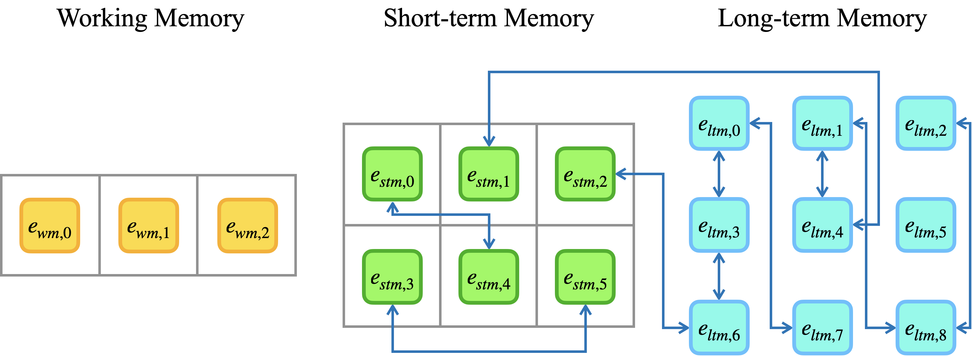
Memoria has three types of memory; working memory (WM), short-term memory (STM), and long-term memory (LTM). Engram, which is the smallest unit of memory information, constitutes each memory. These engrams have their own lifespan and are eliminated when their lifespan reaches zero. Figure 1 shows the structure of the three types of memory.

Memory Encoder A memory encoder $f_{e}$ is needed to transform the input $X_{t}$ into engrams at a particular time step. The design of the memory encoder can vary, and $X_{t}$ was defined as the model hidden states of each time step in our work. The output of $f_{e}$ is a set of engrams $M=\{e_{1},e_{2},\dots,e_{N}\}$.

Working Memory Working memory represents the most recent memory and serves as a reference to retrieve associated engrams from short-term and long-term memory. Working memory adopts a queue structure with a fixed size of the number of newly created engrams in a time step. After every time step, the working memory is updated.

Short-term Memory Short-term memory $M_{stm}$ holds recent information with an adjustable capacity. The engrams in working memory are transferred to short-term memory after a time step. Short-term memory employs a queue data structure with a fixed size.

Long-term Memory Long-term memory $M_{ltm}$ has the capacity to store an indefinite number of engrams. The dequeued engrams from short-term memory are transferred to long-term memory. The age of engrams in the long-term memory can vary considerably.

Memory Graph Engrams in any memory can be connected together, represented as a directed weighted graph data structure, where each vertex corresponds to an engram. A directed edge weight $E_{i\rightarrow j}$ denotes the empirical conditional probability that the engram $e_{j}$ will be retrieved when the engram $e_{i}$ is already retrieved, with $M^{rem}$ representing the set of all retrieved engrams. This empirical probability can be calculated by dividing the number of times $e_{i}$ and $e_{j}$ were retrieved together by the number of times $e_{i}$ was retrieved. $Count_{i,j}$ represents the number of times $e_{i}$ and $e_{j}$ were retrieved together. The edge is utilized to search for engrams in the long-term memory and its weight is adjusted based on the “fire together, wire together” principle (Hebb, 1949). The graph structure depicting the interconnectivity among engrams reflects the association weights between items in SAM (Raaijmakers & Shiffrin, 1981; Kahana, 2020) and plays a crucial role in addressing Memory Searching problem.

$$E_{i\rightarrow j} =P(e_{j}\in M^{rem}\mid e_{i}\in M^{rem})$$

$$=\frac{Count_{i,j}}{Count_{i,i}}$$

3.2 Retrieve

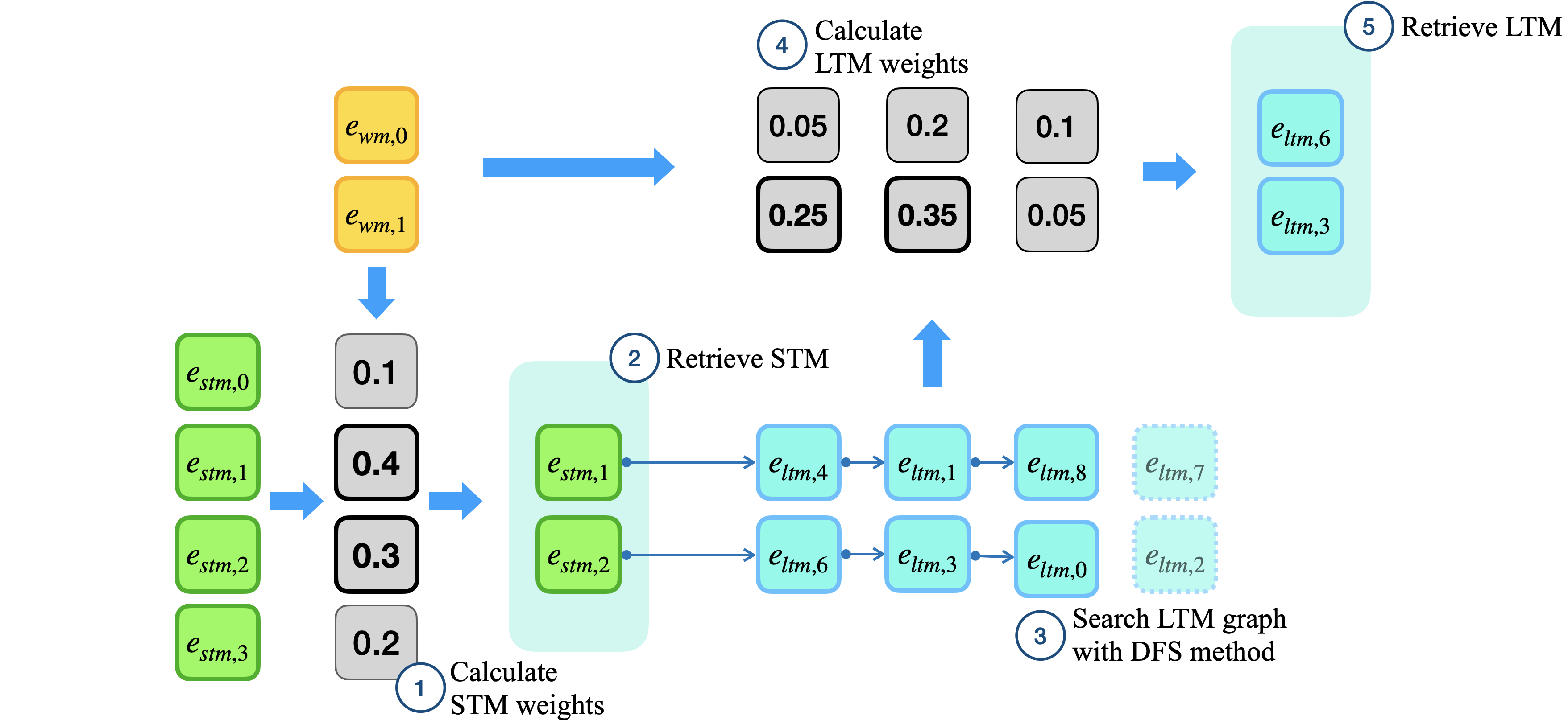
Retrieve is the process of retrieving engrams from short-term and long-term memory. Figure 2 shows entire retrieving process.

1. Using the encoder function $f_{e}$ with input $X$, create engrams $M_{wm}$ and put into the working memory. All the engrams in the working memory will have the same initial lifespan.

   $$M_{wm}=f_{e}(X)=\{e_{wm,1},e_{wm,2},\dots,e_{wm,N_{wm}}\}$$

2. By utilizing the correlation function $f_{c}$, calculate the correlation weight $C_{stm}$ for each $e_{stm,i}$ within the short-term memory $M_{stm}$ by averaging all the correlation weights for the engram. The distance function $f_{d}$ used is L2 distance. Here, $i$ represents the index of $M_{stm}$ and $j$ represents the index of $M_{wm}$.

   $$f_{c}(e_{i},e_{j}) =\mathrm{exp}(-(f_{d}(e_{i},e_{j}))^{2})$$

   $$C_{stm,i} =\frac{1}{N_{wm}}\sum_{j=1}^{N_{wm}}f_{c}(e_{stm,i},e_{wm,j})$$

3. Select only the top $N_{stm}^{rem}$ number of engrams with $C_{stm}$ values to retrieve. Denote the selected engrams as $M_{stm}^{rem}$.

4. For each $e_{i}\in M_{stm}^{rem}$, select an engram in $M_{ltm}$ having highest edge weight from $e_{i}$. Denote the selected engrams as $M_{ltm}^{init}$.

   $$M_{ltm}^{init}=\operatorname*{arg\,max}_{e_{j}\in M_{ltm}}E_{i\rightarrow j},\ \textrm{where }e_{i}\in M_{stm}^{rem}$$

5. Using the engrams $M_{ltm}^{init}$ as a starting point, traverse the $M_{ltm}$ graph using the depth-first search (DFS) algorithm with a search depth of $N_{depth}$. The exploration direction should be based on the edge weight, toward the highest edge weight. Gather all the unique engrams that were encountered during the search, including $M_{ltm}^{init}$, and refer to them as $M_{ltm}^{found}$.

   $$M_{ltm}^{0}=M_{ltm}^{init}$$

   $$M_{ltm}^{k}=\operatorname*{arg\,max}_{e_{j}\in M_{ltm}}E_{i\rightarrow j},$$

   $$\textrm{ where }e_{i}\in M_{ltm}^{k-1},\ e_{j}\notin M_{ltm}^{found,k-1}$$

   $$M_{ltm}^{found,k}=\bigcup\limits_{l=0}^{k}M_{ltm}^{l}$$

   $$M_{ltm}^{found}=M_{ltm}^{found,N_{depth}}$$

6. Calculate correlation weight $C_{ltm}$ from $M_{wm}$ for $M_{ltm}^{found}$ and select top $N_{ltm}^{rem}$ number of engrams like STM. Denote the engrams as $M_{ltm}^{rem}$.

7. Use $M_{wm},M_{stm}^{rem},M_{ltm}^{rem}$ as activated memory.

   $$M^{rem} =M_{stm}^{rem}\cup M_{ltm}^{rem}$$

   $$M^{act} =M_{wm}\cup M^{rem}$$

Through a mechanism in which the final activation is determined based on the weight with working memory, Cue-based Activation is achieved. Memory Searching can be conducted effectively without accessing the entire long-term memory by iteratively exploring new engrams based on the already found engrams and their connection weights.

3.3 Exploit

Exploit all the retrieved engrams to aid in solving the task and evaluate each engram’s contribution. A cross-attention mechanism is applied to utilize engrams. The average attention weight $w_{i}$ for each engram $e_{i}$ is regarded as its contribution towards the solution.

Figure 4: Results of sorting task. Memoria shows more robust performances than other baselines as the input sequence length increases. Considering the nature of the task that requires the retention of information about the occurrence of initial tokens until the end, Memoria demonstrates effectively solving the issue of fateful forgetting compared to competing techniques. The entire raw scores are specified in Table 4.

3.4 Memorize & Forget

In this stage, while accomplishing Selective Preservation, it also strengthens the connections among associated engrams. Figure 3 shows the overall process in this stage.

1. Increase $Count_{i,j}$ by one for all engrams in $M^{act}$, which is the number of times $e_{i}$ and $e_{j}$ retrieved together.

   $$\mathcal{N}=\{1,2,\dots,|M^{act}|\}$$

   $$Count_{i,j}:=Count_{i,j}+1,\forall i,j\in\mathcal{N}$$

2. Increase lifespan of retrieved engrams by the increment ${Inc}_{i}$ for the engram $e_{i}$. ${Inc}_{i}$ is calculated as follows where $\alpha$ is hyperparameter meaning lifespan extend scale. If $\alpha$ is 1.0, each engram $e\in M^{rem}$ gets lifespan 1.0 on average.

   $${Inc}_{i}=\frac{w_{i}}{\sum_{k=1}^{|M^{rem}|}w_{k}}\times|M^{rem}|\times\alpha$$

3. Decrease lifespan of all engrams by 1.0.

4. Remove engrams having a lifespan of 0 or less.

5. Move $e_{wm}$ into STM.

6. Move oldest engrams from STM by the number exceeding capacity into LTM.

The differentiation in the lifespan occurs at two levels. First, engrams that are not retrieved fail to acquire lifespan and are soon eliminated. Additionally, retrieved engrams receive varying lifespans based on their contribution, leading to Selective Preservation at two levels. The connections among retrieved engrams are strengthened, facilitating co-retrieval of more closely associated engrams in Memory Searching.

4 Experiments

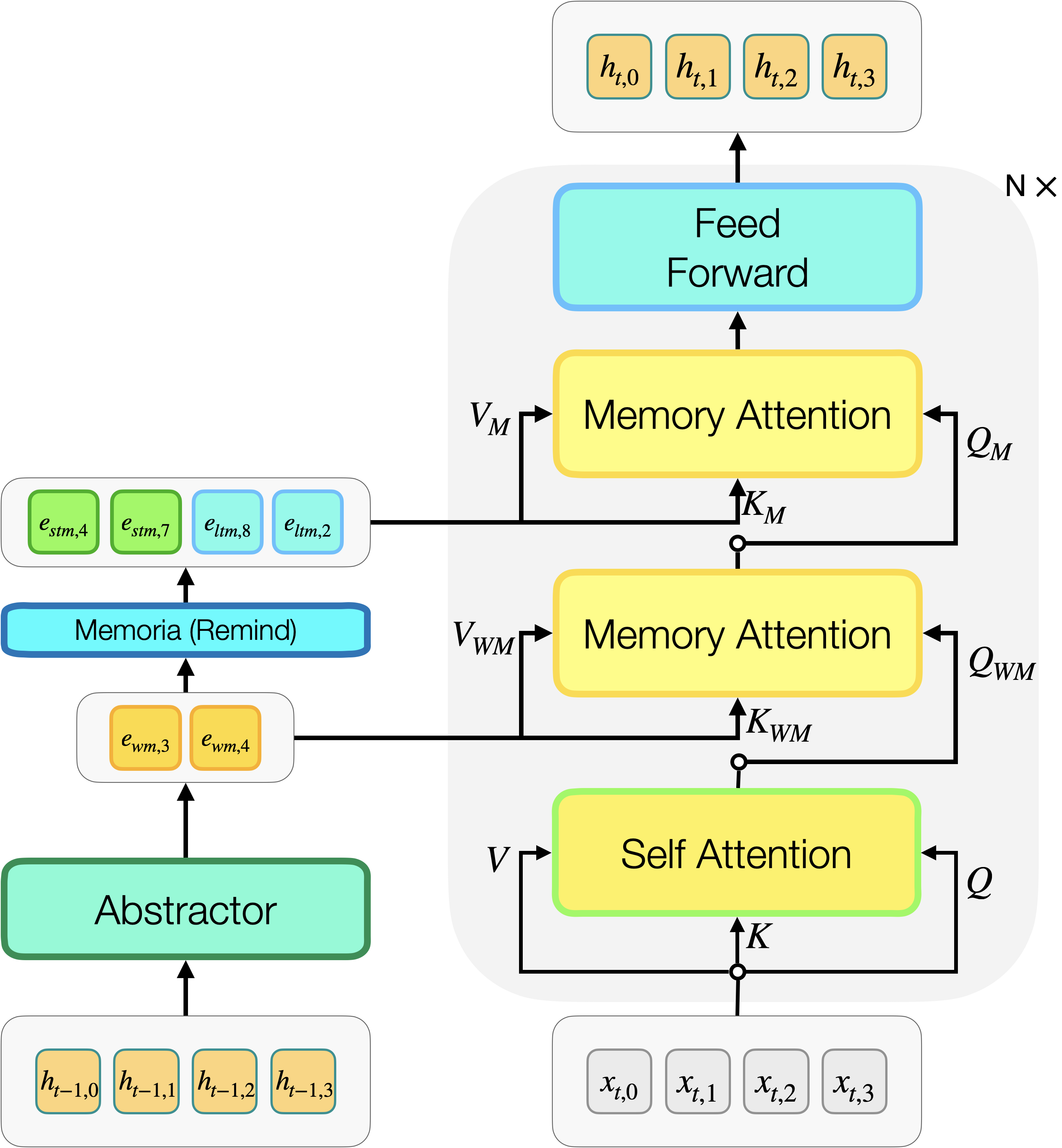
We applied Memoria to the Transformer and evaluated its ability to capture long-term dependencies in various tasks. We provide figures with descriptions representing how to apply Memoria to Transformer in Appendix F. The first task is sorting. Martins et al. (2021) evaluated the model’s ability to remember long-term information about the occurrence of numbers by generating a sorted sequence of numbers based on their frequency of occurrence. In the second group of experiments, we focused on language modeling task for token-level on WikiText-103 (Raw) (Merity et al., 2017) and PG-19 (Rae et al., 2020), and character-level on enwik8 (Mahoney, 2006). Similar to Martins et al. (2021), only the first 2,000 books of the training dataset were used for PG-19. We compared Memoria with other models such as Transformer (Brown et al., 2020), Transformer-XL (Dai et al., 2019), Compressive Transformer (Rae et al., 2020), and $\infty$-former (Martins et al., 2021). Lastly, we conducted a classification task on the long document classification dataset, Hyperpartisan (Kiesel et al., 2019). Appendix B provides additional experiments and detailed hyperparameters for each task.

4.1 Sorting

Table 1: Language Modeling Performance. Perplexity (PPL) is shown for Wikitext-103 and PG-19, while bits-per-character (BPC) is shown for Enwik8. All of them had the same memory length as the segment length, and Wikitext-103 and PG-19 used 150 while Enwik8 used 512. Memory Transformer has achieved the best performance among all models.

Model	Wikitext-103 (PPL)	PG-19 (PPL)	Enwik8 (BPC)
Transformer	26.755	31.631	1.28
Transformer-XL	24.543	29.945	1.19
Compressive Transformer	24.794	29.603	1.16
$\infty$-former	24.685	29.154	1.21
Memoria Transformer	23.471	29.149	1.16

Figure 5: The average age of retrieved engrams in the long-term memory. The age of retrieved engrams gradually increased as steps passed by. This manifests that Memoria is retaining and utilizing not only recent memories but also old memories.

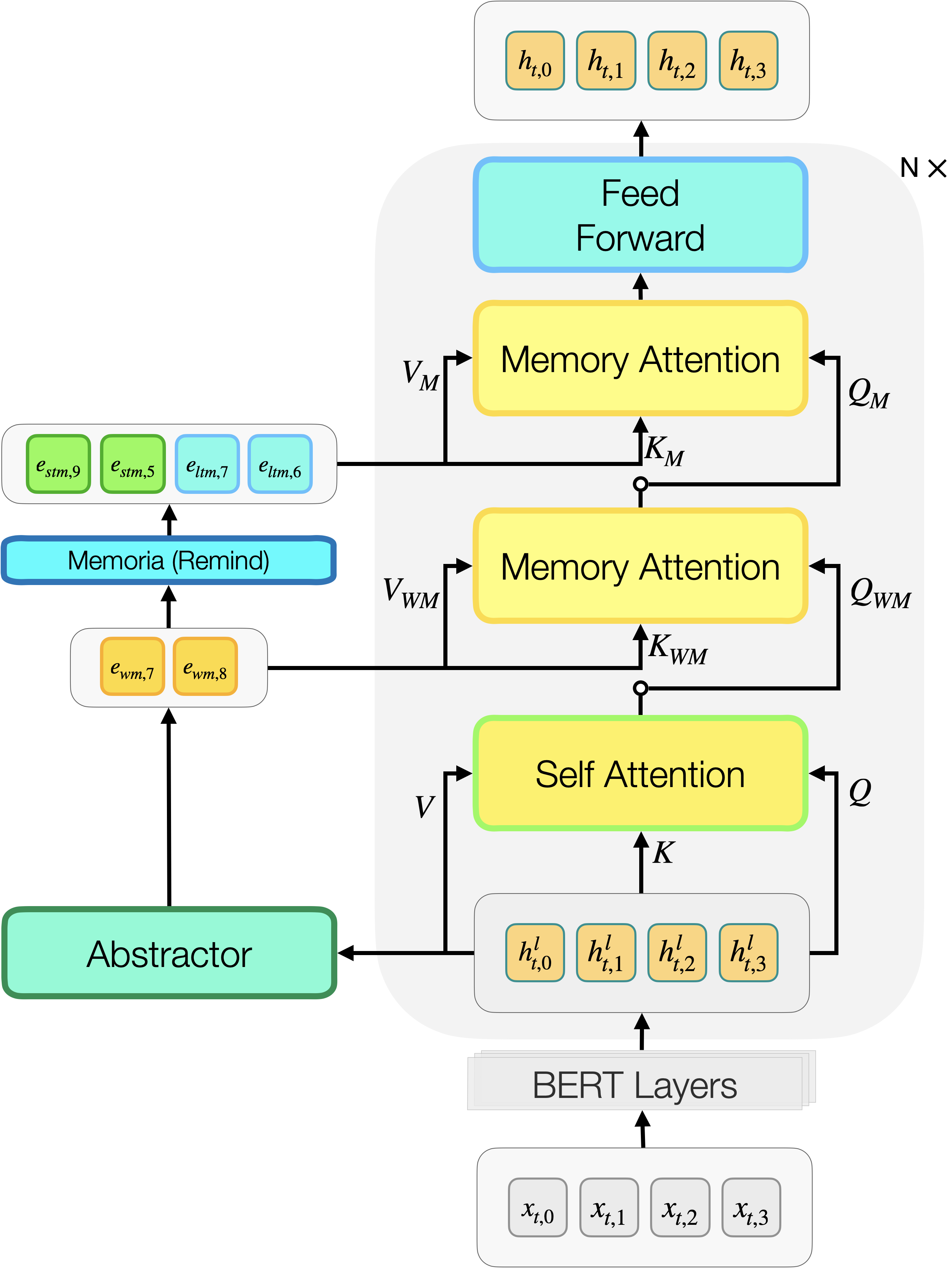
As Memoria is an independent module that enhances long-term dependencies, in order to apply Memoria to Transformer, we needed to define the memory encoder $f_{e}$ and a method that utilizes the retrieved engram data. We used the attention-based abstractor as $f_{e}$ and the last hidden state of the previous time step of the model as $X_{t}$. The hidden states $h_{t-1}$ of the previous time step are used as $X_{t}$. The three values of $Q$, $W_{k}$, and $W_{v}$ are trainable parameters. FFN is a feed-forward network as same in Transformer (Vaswani et al., 2017). The number of working memory engrams $N_{wm}$ is determined by the number of queries $Q$, so the number of queries is a hyperparameter.

$$X_{t} =h_{t-1}$$

$$f_{e}(X_{t}) =\textrm{Abstract}(X_{t})$$

$$=\textrm{FFN}(\textrm{Attention}(Q,W_{k}X,W_{v}X))$$

$$=\textrm{FFN}(\textrm{Attention}(Q,W_{k}h_{t-1},W_{v}h_{t-1}))$$

$$=\textrm{FFN}(\textrm{softmax}(QW_{k}h_{t-1})W_{v}h_{t-1})$$

$$=M_{wm}$$

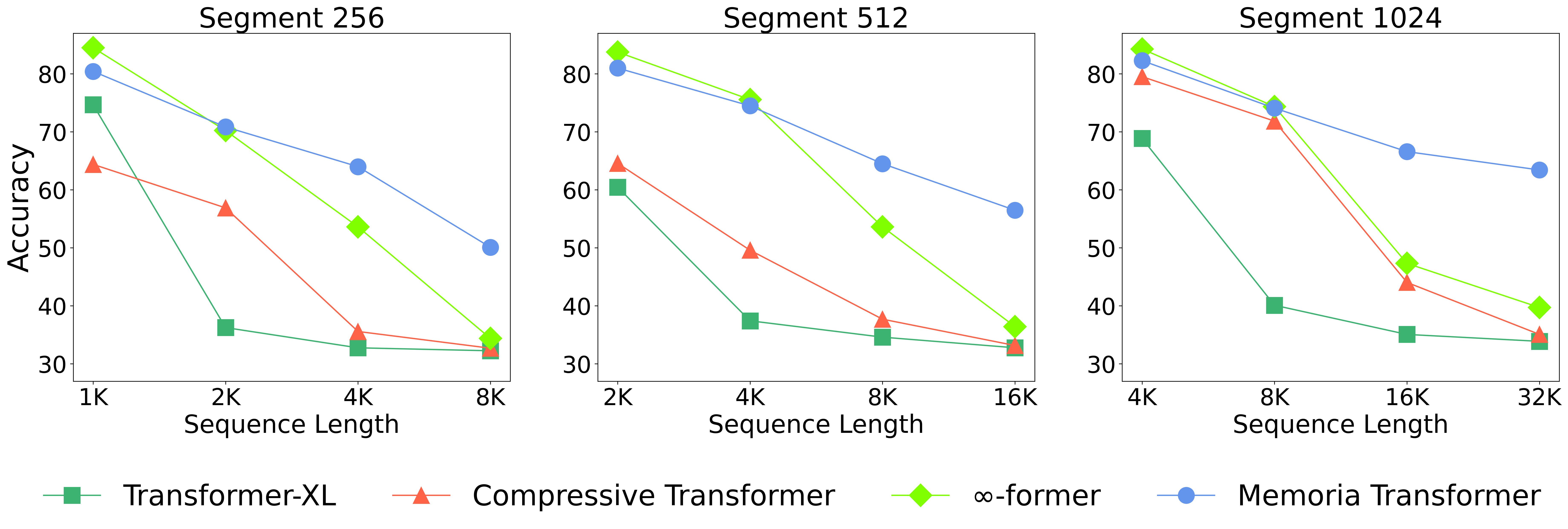
This task is about taking a sequence of numbers and outputting the numbers in descending order of their frequency of occurrence (Martins et al., 2021). The vocabulary consists of 20 number tokens, and we experimented with sequences of various lengths ranging from 1K to 32K, with segment lengths of 256, 512, and 1024. In this task, maintaining the initial information until the end is essential for addressing fateful forgetting, as the occurrence frequencies of each token vary between the initial and final stages.

Figure 4 demonstrates the performance in the sorting task as sequence length increases for each segment length. The memory length was set to the same value as the segment length. Generally, as the sequence length increased, the performance tended to decrease because longer context information needs to be maintained. Compared to the other two models, Memoria exhibited the least performance degradation as the sequence length increased, showcasing its ability to maintain long-term memory for preserving extended context. To understand the respective roles of each memory, we conducted an ablation study in Appendix C using datasets of various lengths. This shows the complementary functions of each memory module.

4.2 Language Modeling

In language modeling as well, Memoria was applied to the Transformer architecture using the same approach as in the sorting task. As publicly available pre-trained models were trained on different datasets and parameters, we conducted this experiment by training models from scratch. We experimented with pre-trained language models equipped with Memoria and showed the results in Section B.2. We utilized GPT-2 architecture with 12 layers and 768 dimensions. The pre-trained GPT-2 tokenizer was used for all token-level experiments. We set the segment length as 150 tokens for token-level experiments and 512 for character-level experiments following the Bulatov et al. (2022).

Table 1 shows the results. All other models demonstrated improved performance compared to Transformer. Among them, Memoria Transformer achieved the best performance on all three datasets. Given that language modeling is more complex than simply capturing long-term context, such outcomes show the effectiveness of Memoria in practical tasks.

Table 2: Perplexity with a smaller segment length of 50. Memoria outperformed other baselines in the shorter context and memory setting.

Model [Memory Length]	Wikitext-103
Transformer	39.287
Transformer-XL [50]	31.459
Compressive Transformer [50]	31.644
$\infty$-former [50]	31.790
Memoria Transformer [48]	30.007

Table 3: Text classification performance on Hyperpartisan. The metrics are average macro F1-score and accuracy of five runs. We reported validation and test set results because of data distribution discrepancy. Memoria RoBERTa achieves the highest performance in the models.

Model [Sequence Length]	Validation		Test
	F1${}_{\pm\text{STD}}$	Acc${}_{\pm\text{STD}}$	F1${}_{\pm\text{STD}}$	Acc${}_{\pm\text{STD}}$
BERT [512]	$76.61_{\pm 0.04}$	$78.75_{\pm 0.03}$	$91.67_{\pm 0.01}$	$93.05_{\pm 0.01}$
RoBERTa [512]	$82.96_{\pm 0.02}$	$84.06_{\pm 0.02}$	$95.24_{\pm 0.02}$	$95.38_{\pm 0.02}$
Bigbird [4096]	$81.22_{\pm 0.02}$	$82.81_{\pm 0.02}$	$93.24_{\pm 0.01}$	$93.54_{\pm 0.01}$
Longformer [4096]	$78.33_{\pm 0.03}$	$79.69_{\pm 0.03}$	$94.56_{\pm 0.01}$	$94.77_{\pm 0.01}$
Memoria BERT [512]	$78.24_{\pm 0.04}$	$80.00_{\pm 0.04}$	$94.59_{\pm 0.02}$	$94.77_{\pm 0.02}$
Memoria RoBERTa [512]	$\textbf{86.39}_{\pm 0.01}$	$\textbf{87.19}_{\pm 0.01}$	$\textbf{96.51}_{\pm 0.02}$	$\textbf{96.62}_{\pm 0.02}$

Table 2 presents the performance measurement in a case where the length of each segment was decreased to 50 tokens, aiming to handle longer long-term dependencies by increasing the number of segments. When comparing the results in Table 1, it is evident that there is a significantly larger performance gap between plain Transformer and the memory utilization models. Even in situations where longer long-term dependencies need to be considered, Memoria demonstrated the best performance.

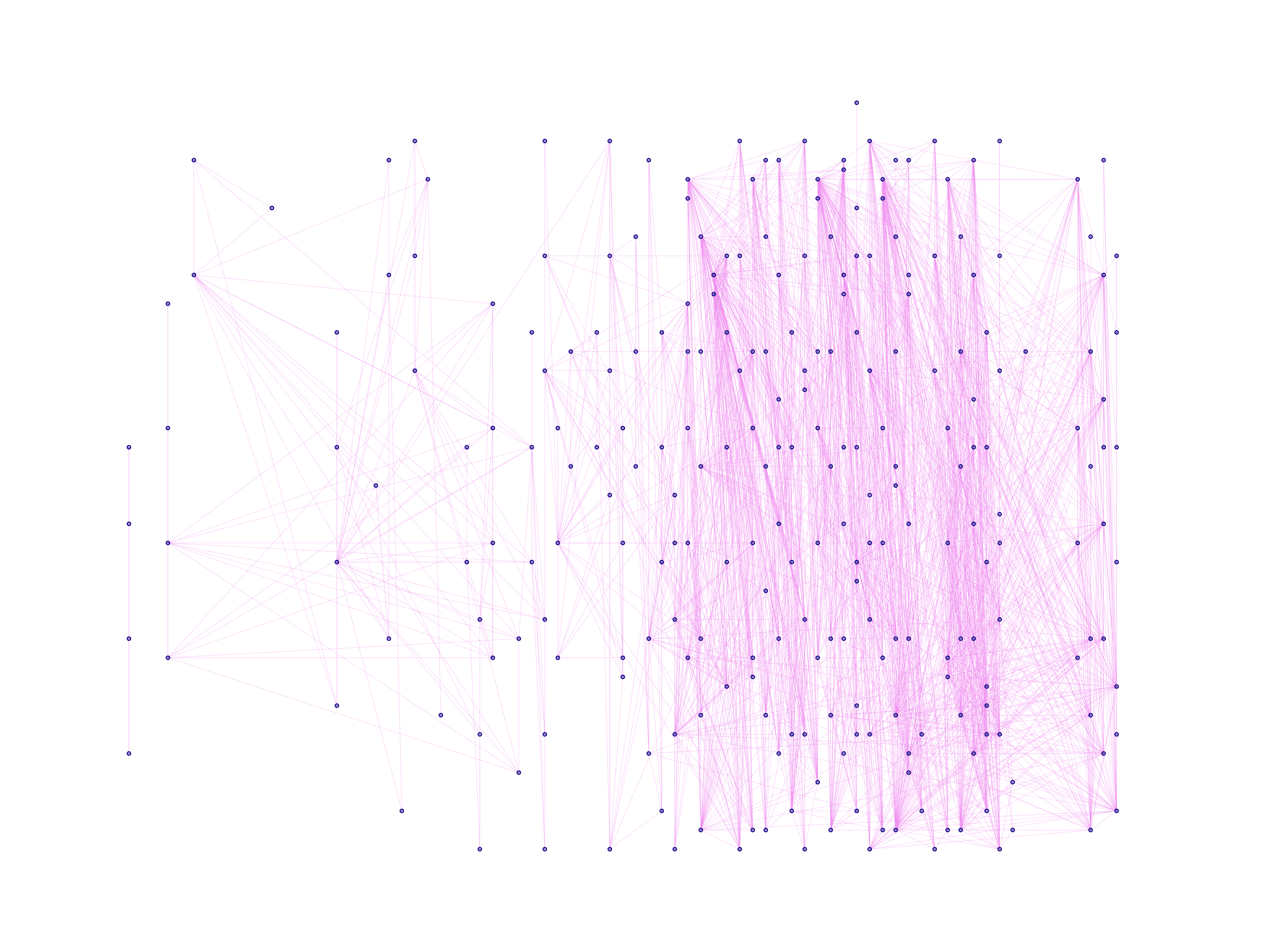
We validated whether Memoria effectively utilizes long-term memory. Figure 5 shows the average age of retrieved engrams in long-term memory at each step on the test dataset. The age represents the number of steps that have passed since the engram was created. If the model only refers to the most recent engram in long-term memory, it would not correctly serve as a long-term memory, and the age of retrieved engrams remains constant on the graph. On the contrary, if the model can refer to past information continuously, the past information will gradually age more, leading to an increase in the average age of retrieved engrams over time. The graph indicates that as the step increases, the average age also increases, demonstrating the ability of Memoria to refer to important past information even after a significant number of time steps. We provided the visualizations of changes of connection in Appendix G to help understand these processes.

4.3 Classification

Utilizing the information from the current time step could lead to causal leakage in language modeling so previous time steps were used as working memory instead. However, with masked language models such as BERT, it is possible to use the information from the current time step as working memory without causing causal leakage. The memory encoder $f_{e}$ utilized the hidden states $h_{t}^{l}$ memory representation. Here, $t$ denotes the current time step, and $l$ represents the memory layer index. Memory is obtained from the hidden state of the BERT layer $l$ with abstractor, and then working memory engrams and retrieved engrams are utilized in the subsequent layers using cross-attention.

Hyperpartisan is a widely used dataset for the long document classification task. To validate the effectiveness of Memoria in encoder-based architectures, we applied Memoria to BERT and RoBERTa and compared its performance. Pre-trained models were used for all the classification experiments. All the models were 12-layer base-sized. Memoria BERT and Memoria RoBERTa utilized 192 memories.

Table 3 presents the classification performance of models. It is evident that Memoria applied models show meaningful performance gains compared to the plain models, although it is not easy to compare the performance of different base pre-trained models directly. Memoria RoBERTa achieved the highest score of all metrics. When conducting a one-tailed t-test, the performance of Memoria RoBERTa was statistically significantly higher than Longformer and Bigbird, with p-values of 0.045 and 0.005, respectively.

5 Conclusion and Future Work

We propose Memoria as a general memory module for neural networks, addressing the fateful forgetting and its derivative problems encountered by existing memory-augmented neural networks in handling long sequential data, particularly the issues of Long-term Importance, Selective Preservation, Cue-based Activation, and Memory Searching. The solutions to these problems draw inspiration from the human memory system, actively incorporating various psychological and neuroscientific theories related to memory, including the Multi-Store Model (Atkinson & Shiffrin, 1968), SAM (Raaijmakers & Shiffrin, 1981), and Hebbian theory (Hebb, 1949). This approach allows Memoria to reflect various human memory effects, including the recency effect, primacy effect, and temporal contiguity effect. We demonstrate these effects through diverse analyses. We applied Memoria to Transformers and demonstrated its strong performance compared to other methodologies in tasks of sorting, language modeling, and classification. We anticipate that Memoria will contribute to the realization of human-level intelligence in diverse sequential processing and agent-based tasks.

We endeavored to empower Memoria with the powerful characteristics of human memory; however, there still exist discrepancies in many aspects. The levels of processing theory (Craik & Lockhart, 1972) proposed a more continuous structure of memory based on the depth of processing rather than discrete categories of the Multi-Store model. The interference theory (Underwood & Postman, 1960) suggests that interference effects between existing memories and new information are significant forgetting mechanisms in long-term memory. Our future research will incorporate these mechanisms into Memoria to better reflect the ways human memory operates and enhance its functionality accordingly.

Impact Statements

This paper aims to develop an external memory module for artificial neural networks, expecting to enhance the processing of diverse long-sequence data. The development of Memoria incorporates theories related to human memory, which may have various societal implications. In particular, Memoria maintains information generated during inference in memory. Therefore, if specific user information is repeatedly used over an extended period for model inference, the accumulated information in Memoria raises concerns regarding regulations on user privacy. Individuals utilizing Memoria should consider reviewing regulations related to personal information.

Appendix A Hebbian Attributes for Memoria

Gerstner & Kistler (2002) suggested six attributes of a useful plasticity model for Hebbian learning as follows. Memoria meets these attributes.

Locality

The learning rule for the synapse $E_{i\rightarrow j}$ connecting neuron $j$ to neuron $i$ should depend only on the activity of $j$ and $i$ and not on the state of other neurons $k\neq i,j$.

$$E_{i\rightarrow j} =\frac{Count_{i,j}}{Count_{i,i}}$$

By definition, Memoria meets locality because it depends on only the count of $i,j$.

Cooperativity

Hebb’s formulation ‘takes part in firing it’ implies that an increase in weight requires both the presynaptic and the postsynaptic neuron to be active.

$$E_{i\rightarrow j}\propto Count_{i,j}$$

Since $E_{i\rightarrow j}$ is proportional to $Count_{i,j}$ and $Count_{i,i}$ never decreases, it only increases when $e_{i}$ and $e_{j}$ fire (retrieved) together.

Synaptic depression

A mechanism for decreasing weights is a necessary requirement for any useful learning rule. There are three engrams $e_{i},e_{j},e_{k}$. $E_{i\rightarrow j}$ decreased when $e_{i}$ and $e_{k}$ fire together while $e_{j}$ does not. The superscript $pre$ means the value before firing of $e_{i}$ and $e_{j}$ and $post$ means the value after firing.

$$E_{i\rightarrow j}^{pre} =\frac{Count_{i,j}^{pre}}{Count_{i,i}^{pre}}$$

$$Count_{i,k}^{post} =Count_{i,k}^{pre}+1$$

$$Count_{i,i}^{post} =Count_{i,i}^{pre}+1$$

$$E_{i\rightarrow j}^{post} =\frac{Count_{i,j}^{post}}{Count_{i,i}^{post}}$$

$$=\frac{Count_{i,j}^{pre}}{Count_{i,i}^{pre}+1}$$

$$<E_{i\rightarrow j}^{pre}$$

Boundedness

In realistic rules, weights should remain bounded in a specific range. $E_{i\rightarrow j}$ must be between 0 and 1 because it is probability.

$$E_{i\rightarrow j}=P(e_{j}\in M^{rem}\mid e_{i}\in M^{rem})$$

$$0\leq P(e_{j}\in M^{rem}\mid e_{i}\in M^{rem})\leq 1$$

Competition

The growth of some weights comes at the cost of a decrease in others. The increase of $E_{i\rightarrow j}$ requires the increase of $Count_{i,j}$ and $Count_{i,i}$. The increase of $Count_{i,i}$ reduces all the weight $E_{i\rightarrow k}$, for $k\neq j$.

Long-term stability

In adaptive systems, it is important to ensure that previously acquired knowledge is not forgotten. In Memoria, $E_{i\rightarrow j}$ is always the result of learning from all past examples because $Count$ is cumulative.

Appendix B Training Details and Additional Results

For all experiments, the Adam optimizer and linear scheduler with warm-up were used, and the gradient clipping was set to a norm of 1.0. One or more NVIDIA A100 or A6000 GPUs were used for training.

B.1 Sorting

For all sorting experiments, a batch size of 32, a warmup rate of 0.06, a learning rate of 2e-4, and an epoch of 5 were used for 80,000 train examples. A memory length was configured to match the segment length. The experiments were conducted on datasets with lengths ranging from 1000 to 32,000. Each example on the datasets was divided into segments of lengths 256, 512, and 1024. For each segment length, combinations of sequence lengths and segment lengths were constructed by varying the number of segments, which were set to 4, 8, 16, and 32. The model configuration used was 5 layers, 4 heads, embedding dimension of 512 Transformer. The compression rate is 4 and the ratio of normal memory and compressed memory is one-to-one for Compressive Transformer.

Memoria parameters used in the experiment were as follows: an initial lifespan of 5, a lifespan extension scale $\alpha$ of 8, and a long-term memory search depth $N_{depth}$ of 10 in all cases. Other parameters are adjusted proportionally to the segment length. the number of working memories $N_{wm}$ set to 1/8 of the segment length, the number of retrieved engrams in short-term memory $N_{stm}^{rem}$ set to 1/4 of the segment length, the number of retrieved engrams in long-term memory $N_{ltm}^{rem}$ set to 5/8 of the segment length, and a capacity of short-term memory set to half of the segment length. The sum of $N_{wm}$, $N_{stm}^{rem}$, and $N_{ltm}^{rem}$ is equal to the segment length.

Table 4 shows the all scores of models in the sorting task. The metric is accuracy. For the convenience of comparison, we marked the number of segments instead of the total sequence length of each dataset. The sequence length can be obtained by multiplying the number of segments by segment length. Memoria Transformer proves its robustness for long-term dependency compared to the other models, especially as the number of segments increases.

Table 4: Accuracy in the sorting task. When the segments increase, Memoria outperforms other baselines.

Model	Segments	Segment Length
		256	512	1024
Transformer-XL	4	74.66	60.46	68.86
Compressive Transformer	4	64.38	64.57	79.51
$\infty$-former	4	84.49	83.75	84.28
Memoria Transformer	4	80.42	80.99	82.27
Transformer-XL	8	36.24	37.41	40.09
Compressive Transformer	8	56.88	49.58	71.84
$\infty$-former	8	70.21	75.55	74.34
Memoria Transformer	8	70.84	74.47	74.08
Transformer-XL	16	32.75	34.59	35.06
Compressive Transformer	16	35.57	37.69	44.03
$\infty$-former	16	53.61	53.61	47.31
Memoria Transformer	16	63.99	64.50	66.58
Transformer-XL	32	32.24	32.76	33.87
Compressive Transformer	32	32.68	33.15	35.07
$\infty$-former	32	34.36	36.41	39.71
Memoria Transformer	32	50.08	56.48	63.42

B.2 Language Modeling

For all language modeling experiments, a batch size of 8 and a warmup rate of 0.06 were used. The model configuration used the settings of GPT-2 small by default. The Wikitext-103 and PG-19 datasets were trained for 3 epochs, while the Enwik8 dataset was trained for 20 epochs. GPT-2 tokenizer was used for all datasets except Enwik8, which was trained at the character level using 204 characters. The default learning rate was 2e-4, but in cases where convergence was challenging, 1e-4 was used. However, for experiments fine-tuning pre-trained models, a learning rate of 5e-5 was used. In the experiments conducted on the Wikitext-103 dataset using Transformer-XL and on the PG-19 dataset using $\infty$-former, as well as the experiment with reduced segment length to 50, both Memoria Transformer and Transformer-XL were trained with a learning rate of 1e-4. The memory length was set to be the same or similar to the segment length. The compression rate is 4 and the ratio of normal memory and compressed memory is one-to-one for Compressive Transformer.

Memoria parameters were set as follows: initial lifespan of 9, lifespan extend scale $\alpha$ of 8, and long-term memory search depth $N_{depth}$ of 10. Furthermore, to prevent potential interference with the learning process, we periodically reset all memory in Memoria every 500 steps during training (1500 steps for enwik8 dataset). This was done to avoid referencing memory generated at stages where learning was insufficient, as it could impede the training progress. For the Wikitext-103 and PG-19 datasets, the number of working memories $N_{wm}$, the number of retrieved engrams in short-term memory $N_{stm}^{rem}$, and the number of retrieved engrams in long-term memory $N_{ltm}^{rem}$ were all set to 50, and a capacity of short-term memory was set to 400. For the Enwik8 dataset, $N_{wm}$, $N_{stm}^{rem}$ and $N_{ltm}^{rem}$ were set to 170, and a capacity of short-term memory was set to 1360. When training on the Wikitext-103 dataset with a reduced segment length of 50, $N_{wm}$, $N_{stm}^{rem}$, and $N_{ltm}^{rem}$ were all set to 16, and the short-term memory capacity was set to 128.

Table 5: Finetuning performance on Wikitext-103.

Model	Wikitext-103
GPT-2	20.498
Memoria GPT-2	18.986
GPT-2 Large	15.332
Memoria GPT-2 Large	13.227
GPT-2 XL	15.254
Memoria GPT-2 XL	13.241

To verify whether Memoria can consider long-term context even when finetuning a pre-trained model, we measured performance on Wikitext-103 dataset by finetuning Memoria GPT-2. The architecture of Memoria GPT-2 is the same as Memoria Transformer. The results are Table 5. Memoria GPT-2 showed significantly better performance than GPT-2. This result suggests that Memoria can be combined with various pre-trained models to increase long-term dependencies. Furthermore, as the use of pre-trained large language models (LLMs) has become prevalent, we conducted experiments to verify whether Memoria can be applied in conjunction with LLMs. We performed experiments using large and xl sized models, and successfully achieved performance improvements when applying Memoria to even larger pre-trained models. This demonstrates the potential for LLMs to benefit from considering longer contexts with the help of Memoria.

Table 6: Performance on Wikitext-103 under various parameter variations.

Initial lifespan	Lifespan extend scale $\alpha$	LTM search depth	Reset Period	$N_{wm}$	$N_{stm}^{rem}$	$N_{ltm}^{rem}$	Perplexity
9	8	10	500	50	50	50	23.471
5							23.485
	4						23.518
		5					23.491
			100				23.407
				100	25	25	23.376
				25	100	25	23.831
				25	25	100	23.670

We conducted additional experiments by modifying various hyperparameters to investigate the sensitivity of hyperparameters. Table 6 shows that there is generally no significant difference in performance compared to what was initially reported in the paper. There were even cases where the performance improved compared to the original scores.

B.3 Classification

All hyperpartisan text classification experiments were conducted with a batch size of 16, a learning rate of 5e-5, and a warmup rate of 0.1. The models were trained for 20 epochs. For BERT, the experiment utilized the pre-trained bert-base-uncased model. As for Longformer, the base model was used in the experiment.

Memoria parameters used in the experiment were as follows: an initial lifespan of 12, a lifespan extension scale $\alpha$ of 8, a long-term memory search depth $N_{depth}$ of 10, the number of working memories $N_{wm}$ set to 64, the number of retrieved engrams in short-term memory $N_{stm}^{rem}$, and the number of retrieved engrams in long-term memory $N_{ltm}^{rem}$ both set to 64, a capacity of short-term memory of 128, and the memory layer index set to 9. This means that the output of the 10th layer is used as memory, and it is referenced in the remaining 2 layers of the model.

Appendix C Ablation Study

Table 7: Performance and performance gain of each memory module according to the length of the dataset. Memoria demonstrates excellent performance maintenance as the sequence length increases, thanks to the complementary functions of each memory module. This observation indicates that while the performance gain of working memory decreases with longer sequence lengths, the performance gain of short-term memory and long-term memory increases.

	4K	8K	16K	32K	48K
Number of Segments	4	8	16	32	47
Accuracy
Transformer	36.19	33.79	31.69	29.94	19.04
+ Working Memory	79.69	70.85	62.21	52.01	34.32
+ Short-term Memory	82.66	76.20	66.37	58.75	54.87
+ Long-term Memory	82.27	74.08	66.58	63.42	63.26
Performance Gain
+ Working Memory	+43.50	+37.06	+30.52	+22.07	+15.28
+ Short-term Memory	+2.79	+5.35	+4.16	+6.74	+20.55
+ Long-term Memory	-0.39	-2.12	+0.21	+4.67	+8.39

We conducted an ablation study to analyze the impact of each type of memory in Memoria on performance. The ablation study was conducted on a sorting task with a segment length of 1024 for each dataset, allowing us to capture tendencies based on the length of the data. Additionally, to further investigate the impact on a longer dataset not covered in the main text, we conducted additional experiments with a 48K dataset. Since the segment length is fixed as 1024, an increase in the dataset length leads to an increase in the number of segments.

The analysis results indicate that each type of memory module contributes to overall performance to some extent. An interesting observation is that as the number of segments increases, the influence of each type of memory on performance changes. Examining the results of the 4K dataset, with a segment length of only 4, it is obvious that the majority of performance improvement is practically facilitated by working memory. However, as the dataset length extends to 8K, 16K, and more, the performance gain through working memory diminishes rapidly. Conversely, with longer sequence lengths, it is observable that the impact of short-term memory and long-term memory on performance gradually becomes more significant. The tendency is similar to humans varying in how long they will remember depending on the situation.

This trend indicates that the model does not uniformly utilize all types of memory but selectively employs memory information based on the characteristics of the task or dataset. If the task can be adequately addressed with an understanding of short contexts, the model primarily utilizes working memory. However, when faced with longer contexts that are challenging to solve with working memory alone, the model seems to develop the ability to leverage short-term or long-term memory. Particularly, observing the transition from 32K to 48K, it is evident that the final performance difference between 32K and 48K is minimal when all memories are utilized, thanks to the complementary roles of short-term and long-term memory compensating for the further exacerbated performance deficiencies in Transformer or working memory. These findings suggest that in order to effectively validate the long-term memory capabilities of the model in the future, tasks and datasets should sufficiently demand dependency on long-term context. Memoria demonstrates consistently robust performance across datasets of varying lengths through the complementary roles of three types of memory.

Appendix D Psychological Memory Effects

D.1 Engram Creation Time

Figure 6: Creation time of the remaining engrams in long-term memory after passing all time steps. The x-axis shows the time of creation as a percentage of the total time steps, and the y-axis is the count of engrams generated at that time. The trend line is the kernel density estimate. This graph demonstrates the patterns of the primacy effect and the recency effect, phenomena observed in human memory, also evident in Memoria.

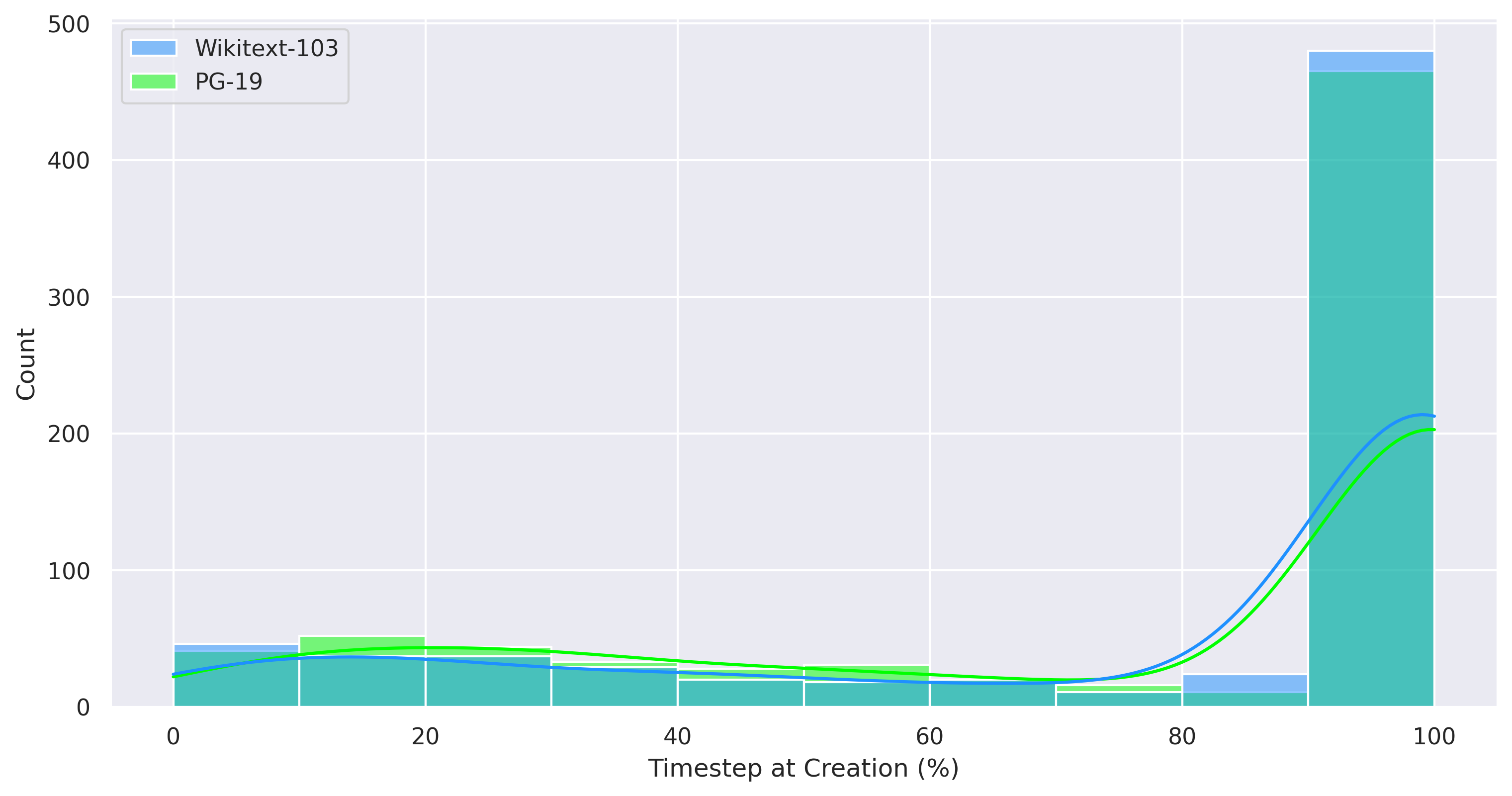
Human memory exhibits various biases when remembering sequentially organized information, and the primacy effect (Deese & Kaufman, 1957; Murdock Jr., 1962) and the recency effect (Bjork & Whitten, 1974; Baddeley & Hitch, 1993) are particularly well-known. The primacy effect is a cognitive bias that refers to the tendency of people to better remember and give greater importance to the first pieces of information, compared to information presented later. This phenomenon is particularly evident in situations where individuals are exposed to a series of items or stimuli, such as a list of words, a sequence of events, or a set of arguments. The recency effect is a cognitive bias that refers to the tendency of individuals to better remember and give more weight to the most recent items or information in a series. In other words, when people are asked to recall a list of items, they are more likely to remember the items that appeared last in the list. This effect can influence various aspects of memory and decision-making. Both the recency and primacy effects are thought to be related to how information is processed and stored in memory. The recency effect is believed to be influenced by short-term memory, where recently presented information is still readily available, while the primacy effect is associated with the transfer of information into long-term memory.

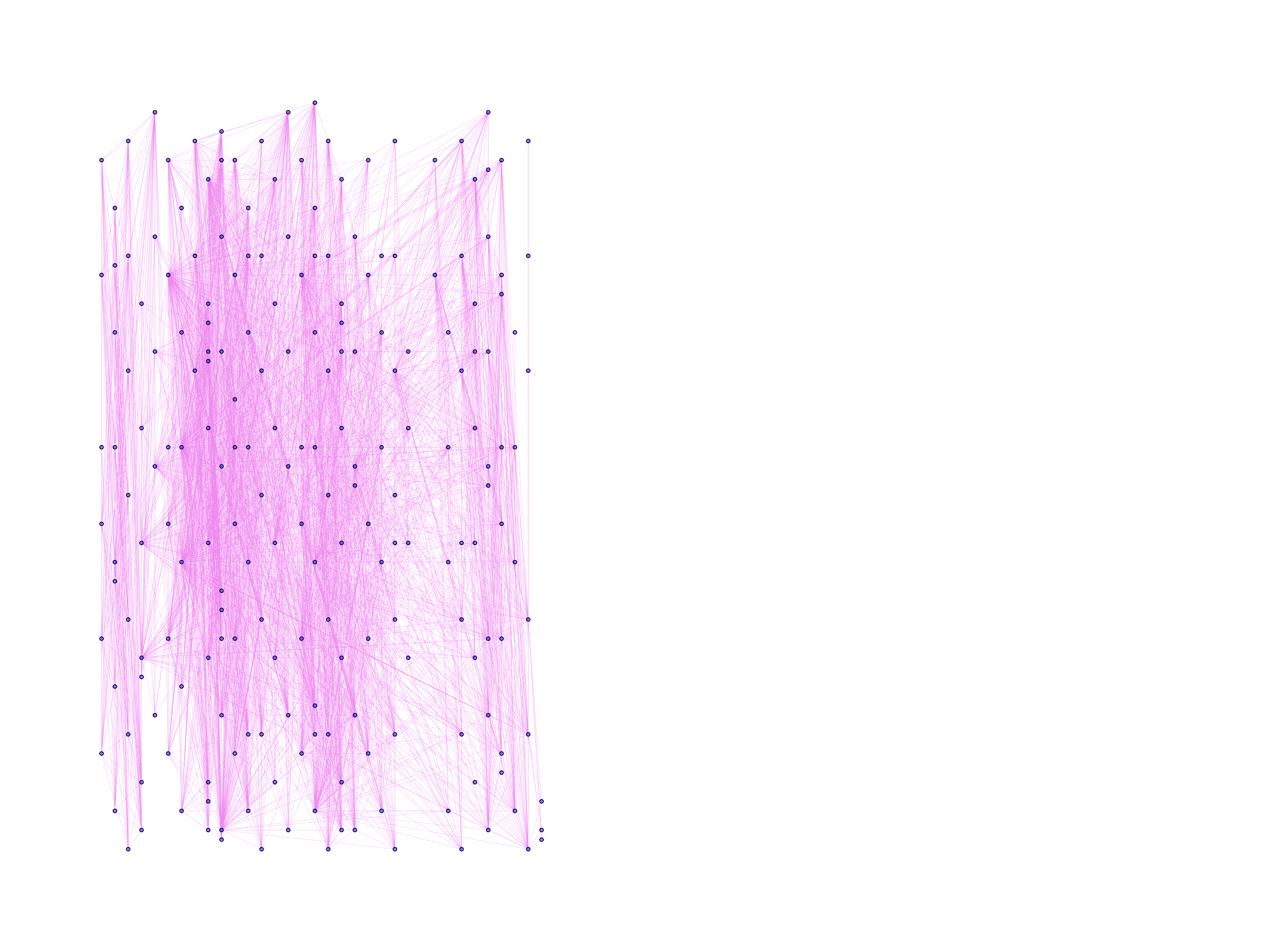
To verify whether these characteristics inherent in humans are also evident in Memoria, we analyzed engrams that persisted in long-term memory after passing all time steps, examining the point in time step when they were created. Figure 6 illustrates the number of remaining engrams at each creation time step. As anticipated, the analysis results demonstrate the presence of both primacy and recency effects in Memoria. In the initial section, there is a clear indication of a primacy effect, as it exhibits a higher count compared to the middle portion. In the later part, there is a substantial difference, with a notably higher count compared to the middle, indicating a pronounced recency effect. In Memoria, early created memories are likely to strengthen through subsequent retrieval, while more recent memories have a high probability of being preserved due to their remaining lifespan. This resembles the primacy effect in humans, where early information tends to be well-maintained due to frequent chances for rehearsal (Rundus & Atkinson, 1970). Additionally, the observed distribution of engrams across the overall time steps in Memoria indicates successful mitigation of the intended “fateful forgetting” issue originally targeted in our objectives.

D.2 Autocorrelation

Table 8: Autocorrelation coefficients of short-term memory and long-term memory engrams.

Lag	Short-term Memory ACF	Long-term Memory ACF
1	0.900	0.575
2	0.893	0.529
3	0.889	0.501
4	0.888	0.475
5	0.888	0.461
6	0.890	0.442
7	0.893	0.426
8	-	0.413
9	-	0.395
10	-	0.381
11	-	0.370
12	-	0.356
13	-	0.344
14	-	0.333
15	-	0.321

In order to identify patterns of retrieved engrams, we conducted autocorrelation analysis using the Wikitext-103 dataset. Table 8 presents the autocorrelation coefficients for short-term and long-term memory. We encoded retrieved engrams as one and others as zero. Lag represents the time step difference for correlation calculation. For instance, the lag of one signifies the autocorrelation between the event of engram $e_{i}$ being retrieved at time $t$ and being retrieved at time $t+1$. For short-lived engrams, with a tendency to be always retrieved or always not, most of those engrams have variances of 0. We regarded the coefficient of these cases as one because it actually means very strong autocorrelations. In addition, for long-term memory, we calculated the weighted average of the correlation coefficients in proportion to the lifespan of each engram, as the total lifespan varies for each engram.

First, looking at short-term memory, the capacity of short-term memory is 400, so each memory stays in short-term memory for 8 times. Therefore, the maximum observable lag is 7. Each engram in short-term memory has a significantly high autocorrelation. This implies that once an engram is retrieved, it is easy for it to be retrieved again, indicating that a specific memory is more frequently associated with others. Long-term memory also shows significant autocorrelation, with high correlation in close time steps decreasing over time. Theoretically, once an engram in long-term memory is retrieved, the association with more recent memories strengthens, making the old memory easier to reach through the pathway of those recent memories. This trend is analogous to the psychological concept of the recency effect (Bjork & Whitten, 1974; Baddeley & Hitch, 1993), where recently encountered information remains more salient. The high autocorrelation in Memoria’s near time steps aligns with this phenomenon. Figure 7 illustrates the changes in autocorrelation based on the lag in long-term memory.

Figure 7: Autocorrelation coefficient plot of long-term memory.

D.3 Association Weights based on Age Differences

Figure 8: A bivariate histogram showing the average weight between all engrams according to the age difference.

Figure 9: Scatterplot of the data in Figure 8 for age differences of 300 or less.

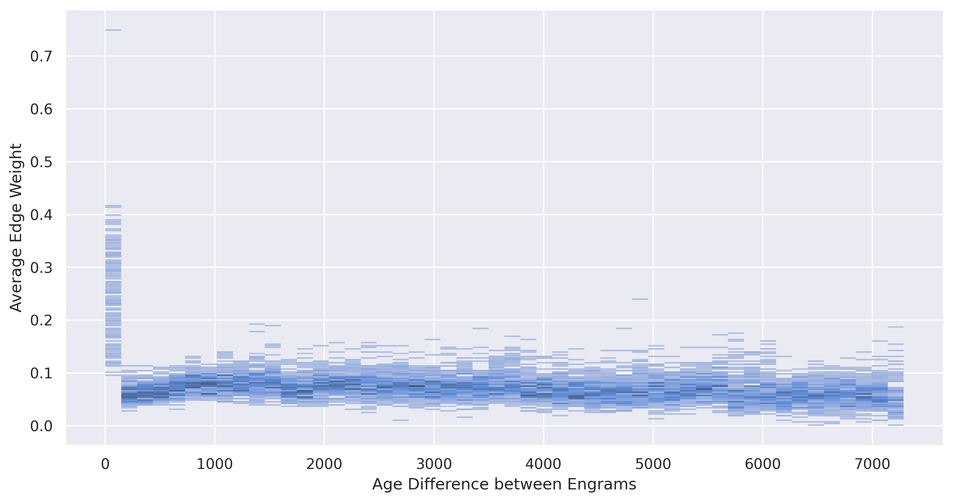
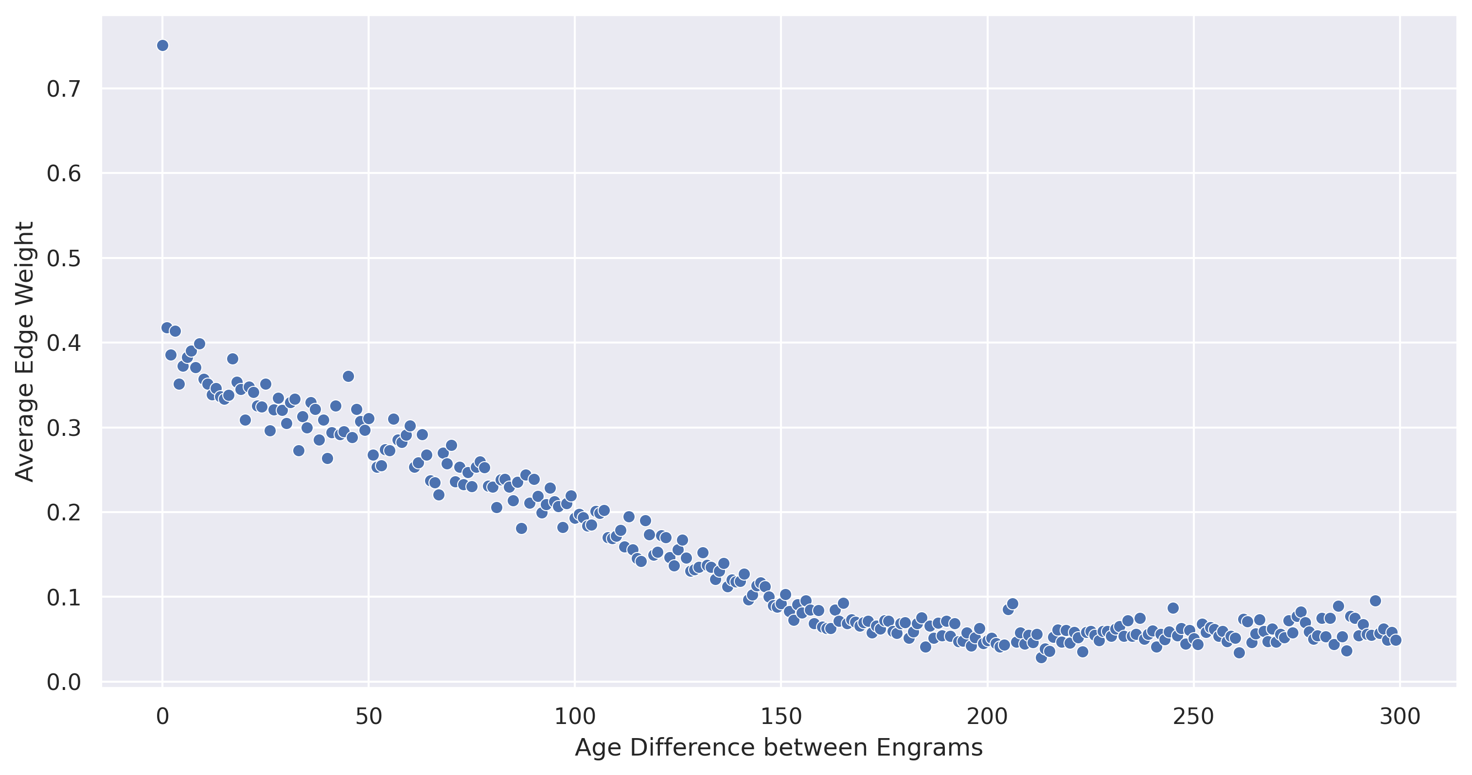
The temporal contiguity effect (Kahana, 1996; Ginns, 2006) refers to a cognitive phenomenon where information is better remembered when elements are presented close in time. In other words, when information is temporally aligned, people tend to have improved memory and comprehension compared to when there is a temporal gap between the presentation of the different elements. This enables capturing the relationships between events that occur in a short period of time for humans.

To investigate the occurrence of the temporal contiguity effect in Memoria, we analyzed the connectivity between remaining engrams in the WikiText-103 test dataset after passing all time steps. We illustrate the changes in average edge weight based on the age difference (temporal gap at the time of creation) between two engrams in Figure 8. The results clearly demonstrate that when the age difference is minimal, there is a significant increase in the average weight, indicating the presence of a temporal contiguity effect in Memoria, strengthening connections between temporally close engrams. Figure 9 is included to finely depict the point where this effect starts to diminish, showing its presence up to approximately 150 age differences. Theoretically, engrams of the same age are more likely to fire together when living in working memory and short-term memory, leading to an increase in the association edge between them.

Appendix E Algorithm & Computational Complexity

E.1 Theoretical Analysis

Each stage of Memoria is represented by an algorithm. These are the algorithms of decoder models in our experiments, so some details might be slightly different from the encoder model’s formula. Additionally, each algorithm provides time complexity to help estimate how many resources are needed.

Algorithm 1 Retrieve Stage

  Input: short-term memory $STM$, long-term memory $LTM$, memory encoder $E$, co-retrieved conditional probabilities $P$, previous hidden states $h_{p}$, long-term memory search depth $N_{depth}$

  Output: working memory $WM$, retrieved engrams $retrieved$

  Result: Encode $h_{p}$ into working memory. Find relevant engrams in the short-term/long-term memories.

  $WM\leftarrow E(h_{p})$

  $W_{stm}\leftarrow CalculateDistance$($STM$, $WM$) {distance from stm to wm}

  $stm_{rem}\leftarrow FindShortestK$($W_{stm}$) {select nearest stms}

  $p\leftarrow GetCondProb$($LTM$, $stm_{rem}$, $P$)

  $ltm_{1}\leftarrow SelectMostProbableEngrams$($p$)

  $ltm_{found}\leftarrow(ltm_{1},)$ 

  for $i\leftarrow 1$ to $N_{depth}$ do

     $p\leftarrow GetCondProb$($LTM$, $ltm_{i}$, $P$)

     $ltm_{i+1}\leftarrow SelectMostProbableEngrams$($p$)

     $Append$($ltm_{found}$, $ltm_{i+1}$)

  end for

  $W_{ltm}\leftarrow CalculateDistance$($ltm_{found}$, $WM$)

  $ltm_{rem}\leftarrow FindShortestK$($W_{ltm}$)

  $retrieved\leftarrow Merge$($stm_{rem}$, $ltm_{rem}$)

The complexity of the $CalculateDistance$ function is equal to the product of the number of engrams in each memory, as it involves the computation of all weights between them. The function is used twice, first in the STM with a time complexity of $O(N_{wm}\times C_{stm})$, where $N_{wm}$ is the number of engrams in working memory and $C_{stm}$ is the capacity of STM. Secondly, when applied to the found LTM, the complexity is $O(N_{wm}\times N_{ltm}^{found})$, where $N_{ltm}^{found}=N_{stm}^{rem}\times(N_{depth}+1)$. The part of the function that retrieves the conditional probability of retrieving the connected LTM engrams given retrieved STM engrams has a complexity of $O(N_{stm}^{rem}\times d)$, where $N_{stm}^{rem}$ is the number of retrieved engrams in STM and $d$ is the degree. The maximum value for degree $d$ is the total number of edges from the engram, resulting in a maximum complexity of $O(N_{stm}^{rem}\times N_{ltm})$. Within the loop that executes $N_{depth}$ times, the complexity is $O(N_{stm}^{rem}\times N_{ltm}\times N_{depth})$. Generally, since the size of LTM is expected to be larger than $N_{wm}$, the overall time complexity of the retrieve stage is $O(N_{stm}^{rem}\times N_{ltm}\times N_{depth})$.

Here, $N_{stm}^{rem}$ and $N_{depth}$ are hyperparameters that can be set directly, but the total number of long-term memory units, $N_{ltm}$, is a dynamically changing value during execution. While it is not possible to precisely determine the size of LTM, the maximum size of LTM over time can demonstrate convergence through lifespan, given a sufficient duration. The increase in lifespan for all engrams during a single execution of the entire memory operations is $\alpha*(N_{stm}^{rem}+N_{ltm}^{rem})$ when alpha represents the lifespan extend scale parameter. Additionally, the decrease in lifespan is the number of all engrams of $N_{ltm}+N_{stm}+N_{wm}$. In a scenario where $N_{ltm}$ is maximized, lifespan is evenly distributed across all engrams, preventing their removal. If the sum of lifespans for all engrams after the nth execution is denoted as $l$, then $N_{ltm}$ can be considered a constant multiple, $l\times c$. However, since the total number of engrams cannot exceed the total lifespan sum, $c$ takes on values between 0 and 1. When memory operations are executed $n$ times, and the total lifespan sum of all engrams is $l_{n}$, $l_{n}$ can be expressed as follows.

$$l_{n+1} =l_{n}+\alpha*(N_{stm}^{rem}+N_{ltm}^{rem})-N_{ltm}$$

$$=l_{n}+\alpha*(N_{stm}^{rem}+N_{ltm}^{rem})-l_{n}\times c$$

$$=(1-c)\times l_{n}+K$$

$$K =\alpha*(N_{stm}^{rem}+N_{ltm}^{rem})$$

$$l_{n+1}-\frac{K}{c} =(1-c)\times(l_{n}-\frac{K}{c})$$

$$b_{n+1} =(1-c)\times b_{n}$$

$$b_{n} =b_{0}\times(1-c)^{n}$$

$$l_{n} =b_{0}\times(1-c)^{n}+\frac{K}{c}$$

$$=b_{0}\times(1-c)^{n}+\frac{\alpha*(N_{stm}^{rem}+N_{ltm}^{rem})}{c}$$

$$\lim_{n\to\infty}l_{n} =\frac{\alpha*(N_{stm}^{rem}+N_{ltm}^{rem})}{c}$$

$$\lim_{n\to\infty}N_{ltm} =\alpha*(N_{stm}^{rem}+N_{ltm}^{rem})$$

Ultimately, when a sufficient amount of time elapses, the overall sum of the lifespan will be proportionate to $\alpha*(N_{stm}^{rem}+N_{ltm}^{rem})$. Therefore, in the worst-case scenario of retrieve stage, the time complexity is as follows.

$$O(N_{stm}^{rem}\times N_{ltm}\times N_{depth}) =O(N_{stm}^{rem}\times(\alpha*(N_{stm}^{rem}+N_{ltm}^{rem}))\times N_{depth})$$

$$=O(\alpha N_{stm}^{rem}N_{depth}(N_{stm}^{rem}+N_{ltm}^{rem}))$$

  Input: model $M$, input segment $s$, $retrieved$

  Output: segment result $r$, hidden states $h_{p}$

  Result: Conduct inference with retrieved memories. Return the segment result, hidden states, and attention weight for each engram.

  $r,h_{p},a\leftarrow M(s,retrieved)$ {”a” means memory attention weights}

Algorithm 2 Exploit Stage

The time complexity of the exploit stage depends upon the way of modeling utilization of retrieved engrams. In our implementation, we have employed a cross-attention method, wherein input data is used as a query for engrams serving as key and value. Consequently, the time complexity aligns with that of cross-attention. The time complexity, given an input length of $L$ and the number of retrieved engrams $N_{e}$, is $O(L\times N_{e})$. $N_{e}$ is equal to $N_{stm}^{rem}+N_{ltm}^{rem}$, so the time complexity is $O(L\times(N_{stm}^{rem}+N_{ltm}^{rem}))$. We configured the total number of engrams used in our experiments to be equal to the sequence length. In this scenario, the time complexity becomes $O(L^{2})$, equivalent to that of self-attention, thereby not exerting an additional impact on the overall time complexity from a Big-O perspective.

  Input: $WM$, $STM$, $LTM$, $P$.

  Output: Updated memories and condition tables.

  $P\leftarrow AdjustConditionalProbs$($P$, $retrieved$) {update probs}

  $IncreaseLifespans$($retrieved$, $a$)

  $STM\leftarrow MoveWMtoSTM$($WM$, $STM$)

  $DecreaseLifespanAndRemove$($STM$, $LTM$)

  $LTM\leftarrow MoveSTMtoLTM$($STM$, $LTM$)

Algorithm 3 Memorize & Forget Stage

The logic governing conditional probability adjustment increases the value for each pair of the retrieved engrams, resulting in a time complexity of $O(N_{e}^{2})$. The logic regulating lifespan, being an operation for each engram, entails a complexity of $O(N_{e})$. Changing the type of memory requires operations proportional to the number of engrams, limiting the complexity to $O(N_{e})$. Consequently, the overall time complexity at this stage is $O(N_{e}^{2})=O((N_{stm}^{rem}+N_{ltm}^{rem})^{2})$.

In Memoria, space complexity is essentially the cost of maintaining a conditional probability table representing the connectivity between each engram. The space complexity is dependent on the implementation of the graph. For the sake of convenient implementation, we have employed the adjacency matrix representation. When using an adjacency matrix, the spatial complexity becomes quadratic in the number of nodes, specifically, the square of the total number of engrams in Memoria, calculated as $O((N_{wm}+C_{stm}+N_{ltm})^{2})$. Alternative implementations such as adjacency lists can further reduce spatial complexity.

Table 9: Time and space complexities on each stage.

Stage	Time Complexity	Space Complexity
Retrieve	$O(N_{stm}^{rem}N_{ltm}N_{depth})$	$O((N_{wm}+C_{stm}+N_{ltm})^{2})$
Exploit	$O(L(N_{stm}^{rem}+N_{ltm}^{rem}))$	$O((N_{wm}+C_{stm}+N_{ltm})^{2})$
Memorize & Forget	$O((N_{stm}^{rem}+N_{ltm}^{rem})^{2})$	$O((N_{wm}+C_{stm}+N_{ltm})^{2})$

Table 9 shows the time complexity and space complexity for each stage using Big-O notation.

E.2 Empirical Analysis

Table 10: Inference time and GPU memory usage

Model	Execution Time (s)	Memory Usage (MB)
Transformer-XL	21.23	525.74
Compressive Transformer	25.57	740.00
$\infty$-former	54.15	676.12
Memoria Transformer	44.21	612.94

In addition to theoretical analysis, we measured the resources used during inference. Table 10 presents the time taken and average memory usage while inferring the Wikitext-103 test set. Regarding execution time, Memoria was faster than the relatively $\infty$-former but slower than the others, while its memory usage was the second smallest. Memory measurements were taken at each step using the functions torch.cuda.empty_cache and torch.cuda.memory_allocated provided by PyTorch, and averages were calculated. In the case of Memoria, there is room for optimizing inference time and memory usage. This can be achieved by uploading information, such as engram type or lifespan, which requires minimal GPU computation, to the CPU. Additionally, optimization of data structures using adjacency lists can be applied. Furthermore, the graph maintained by Memoria does not necessarily need to be implemented using PyTorch or Python, allowing for increased computational efficiency through the use of more efficient programming languages.

Appendix F Memoria applied Transformers

F.1 Memoria Transformer

Figure 10: Architecture of Memoria Transformer. $t$ represents the current time step, and $x$ is the input embedding. The residual network and layer normalization are omitted for clarity. Memoria Transformer creates engrams from the previous time step output $h_{t-1}$ and retrieves engrams from short-term and long-term memory. Memoria Transformer exploits the engrams with cross attention. Memory Attention, depicted as two blocks in the diagram, is actually a single layer that shares the same weights.

F.2 BERT with Memoria

Figure 11: Architecture of BERT with Memoria. $t$ represents the current time step, and $x$ is the input embedding. The residual network and layer normalization are omitted for clarity. In BERT, unlike in GPT-2, engrams are created using information from the current time step. $l$ represents the memory layer index, and from layer 1 to layer $l$, each layer is identical to a regular BERT layer. Using the output $h_{t}^{l}$ from layer $l$, engrams are created and retrieved from short-term and long-term memory. These engrams are then utilized in the subsequent layers (after layer $l$) through cross-attention. Memory Attention blocks, depicted as two blocks in the diagram, actually share the same weights.

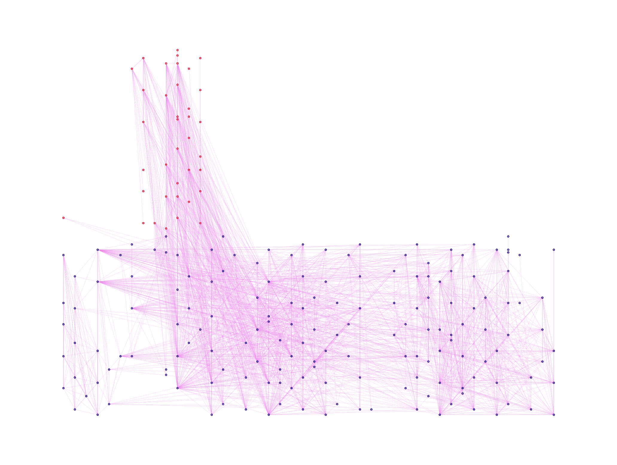
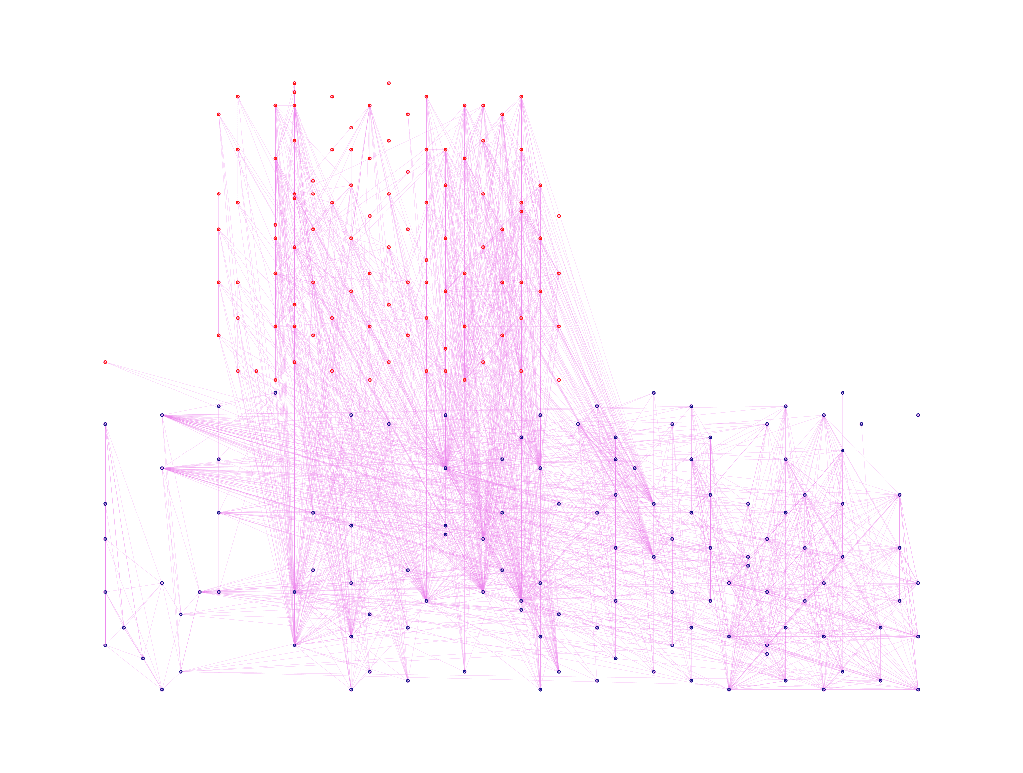
Appendix G Visualization of Memoria

(a) $t=20$

(b) $t=60$

(c) $t=130$

Figure 12: Changes in engrams of Memoria over time. The dots represent engrams, and the lines represent connections between engrams. $t$ is the time step. The more engrams on the right, the later it was created. Only the connections with high weights are shown for clarity. The engrams gradually fade away but some important engrams still remain for a longer duration. The nearby connections are similar to the temporal contiguity effect (Kahana, 1996) of humans. This demonstrates Memoria’s ability to preserve information, even if it has been a long time, as long as it remains useful.

(a) $t=87$

(b) $t=105$

(c) $t=122$

Figure 13: Changes in engrams of Memoria over time when Memoria sees the same data twice. The lower half of each image represents the engrams generated when observing at first, while the upper half represents the engrams generated when observing at second. Thus, the dots in the same vertical column represent engrams created from the same data. Engrams from the same data exhibit a generally stronger connectivity. This means that Memoria can form connections between similar information even if they are temporally distant.

References

- Antony et al. (2017) Antony, J. W., Ferreira, C. S., Norman, K. A., and Wimber, M. Retrieval as a fast route to memory consolidation. Trends in cognitive sciences, 21(8):573–576, 2017.
- Atkinson & Shiffrin (1968) Atkinson, R. and Shiffrin, R. Human memory: A proposed system and its control processes. volume 2 of Psychology of Learning and Motivation, pp. 89–195. Academic Press, 1968. doi: https://doi.org/10.1016/S0079-7421(08)60422-3. URL https://www.sciencedirect.com/science/article/pii/S0079742108604223.
- Atkinson & Juola (1974) Atkinson, R. C. and Juola, J. F. Search and decision processes in recognition memory., pp. xiii, 299–xiii, 299. Contemporary developments in mathematical psychology: I. Learning, memory and thinking. W. H. Freeman, Oxford, England, 1974. ISBN 0716708485.
- Atkinson et al. (1974) Atkinson, R. C., Hermann, D. J., and Wescourt, K. T. Search processes in recognition memory., pp. xi, 386–xi, 386. Theories in cognitive psychology: The Loyola Symposium. Lawrence Erlbaum, Oxford, England, 1974. ISBN 0470812281.
- Baddeley & Hitch (1993) Baddeley, A. D. and Hitch, G. The recency effect: Implicit learning with explicit retrieval? Memory & Cognition, 21(2):146–155, 1993. doi: 10.3758/BF03202726. URL https://doi.org/10.3758/BF03202726.
- Banino et al. (2020) Banino, A., Badia, A. P., Köster, R., Chadwick, M. J., Zambaldi, V., Hassabis, D., Barry, C., Botvinick, M., Kumaran, D., and Blundell, C. Memo: A deep network for flexible combination of episodic memories. In International Conference on Learning Representations, 2020. URL https://openreview.net/forum?id=rJxlc0EtDr.
- Beltagy et al. (2020) Beltagy, I., Peters, M. E., and Cohan, A. Longformer: The long-document transformer. CoRR, abs/2004.05150, 2020. URL https://arxiv.org/abs/2004.05150.
- Bjork & Whitten (1974) Bjork, R. A. and Whitten, W. B. Recency-sensitive retrieval processes in long-term free recall. Cognitive Psychology, 6(2):173–189, 1974. ISSN 0010-0285. doi: https://doi.org/10.1016/0010-0285(74)90009-7. URL https://www.sciencedirect.com/science/article/pii/0010028574900097.
- Braun et al. (2018) Braun, E. K., Wimmer, G. E., and Shohamy, D. Retroactive and graded prioritization of memory by reward. Nature Communications, 9(1):4886, 2018. doi: 10.1038/s41467-018-07280-0. URL https://doi.org/10.1038/s41467-018-07280-0.
- Brown (1958) Brown, J. Some tests of the decay theory of immediate memory. Quarterly Journal of Experimental Psychology, 10(1):12–21, 1958. doi: 10.1080/17470215808416249. URL https://doi.org/10.1080/17470215808416249.
- Brown et al. (2020) Brown, T., Mann, B., Ryder, N., Subbiah, M., Kaplan, J. D., Dhariwal, P., Neelakantan, A., Shyam, P., Sastry, G., Askell, A., Agarwal, S., Herbert-Voss, A., Krueger, G., Henighan, T., Child, R., Ramesh, A., Ziegler, D., Wu, J., Winter, C., Hesse, C., Chen, M., Sigler, E., Litwin, M., Gray, S., Chess, B., Clark, J., Berner, C., McCandlish, S., Radford, A., Sutskever, I., and Amodei, D. Language models are few-shot learners. In Larochelle, H., Ranzato, M., Hadsell, R., Balcan, M., and Lin, H. (eds.), Advances in Neural Information Processing Systems, volume 33, pp. 1877–1901. Curran Associates, Inc., 2020. URL https://proceedings.neurips.cc/paper_files/paper/2020/file/1457c0d6bfcb4967418bfb8ac142f64a-Paper.pdf.
- Bulatov et al. (2022) Bulatov, A., Kuratov, Y., and Burtsev, M. Recurrent memory transformer. In Koyejo, S., Mohamed, S., Agarwal, A., Belgrave, D., Cho, K., and Oh, A. (eds.), Advances in Neural Information Processing Systems, volume 35, pp. 11079–11091. Curran Associates, Inc., 2022. URL https://proceedings.neurips.cc/paper_files/paper/2022/file/47e288629a6996a17ce50b90a056a0e1-Paper-Conference.pdf.
- Burtsev & Sapunov (2020) Burtsev, M. S. and Sapunov, G. V. Memory transformer. CoRR, abs/2006.11527, 2020. URL https://arxiv.org/abs/2006.11527.
- Caporale & Dan (2008) Caporale, N. and Dan, Y. Spike timing-dependent plasticity: a hebbian learning rule. Annu Rev Neurosci, 31:25–46, 2008.
- Chung et al. (2014) Chung, J., Gülçehre, Ç., Cho, K., and Bengio, Y. Empirical evaluation of gated recurrent neural networks on sequence modeling. CoRR, abs/1412.3555, 2014. URL http://arxiv.org/abs/1412.3555.
- Craik & Lockhart (1972) Craik, F. I. and Lockhart, R. S. Levels of processing: A framework for memory research. Journal of Verbal Learning and Verbal Behavior, 11(6):671–684, 1972. ISSN 0022-5371. doi: https://doi.org/10.1016/S0022-5371(72)80001-X. URL https://www.sciencedirect.com/science/article/pii/S002253717280001X.
- Dai et al. (2019) Dai, Z., Yang, Z., Yang, Y., Carbonell, J., Le, Q. V., and Salakhutdinov, R. Transformer-xl: Attentive language models beyond a fixed-length context. ACL 2019 - 57th Annual Meeting of the Association for Computational Linguistics, Proceedings of the Conference, pp. 2978–2988, 1 2019. doi: 10.48550/arxiv.1901.02860. URL https://arxiv.org/abs/1901.02860v3.
- Davis et al. (2014) Davis, T., Xue, G., Love, B. C., Preston, A. R., and Poldrack, R. A. Global neural pattern similarity as a common basis for categorization and recognition memory. Journal of Neuroscience, 34(22):7472–7484, 2014. ISSN 0270-6474. doi: 10.1523/JNEUROSCI.3376-13.2014. URL https://www.jneurosci.org/content/34/22/7472.
- Deese & Kaufman (1957) Deese, J. and Kaufman, R. A. Serial effects in recall of unorganized and sequentially organized verbal material. Journal of Experimental Psychology, 54(3):180–187, 1957. ISSN 0022-1015(Print). doi: 10.1037/h0040536. URL https://doi.org/10.1037/h0040536.
- Devlin et al. (2019) Devlin, J., Chang, M.-W., Lee, K., and Toutanova, K. BERT: Pre-training of deep bidirectional transformers for language understanding. In Proceedings of the 2019 Conference of the North American Chapter of the Association for Computational Linguistics: Human Language Technologies, Volume 1 (Long and Short Papers), pp. 4171–4186, Minneapolis, Minnesota, June 2019. Association for Computational Linguistics. doi: 10.18653/v1/N19-1423. URL https://aclanthology.org/N19-1423.
- Gerstner & Kistler (2002) Gerstner, W. and Kistler, W. M. Mathematical formulations of hebbian learning. Biological Cybernetics, 87(5):404–415, 2002. doi: 10.1007/s00422-002-0353-y. URL https://doi.org/10.1007/s00422-002-0353-y.
- Ginns (2006) Ginns, P. Integrating information: A meta-analysis of the spatial contiguity and temporal contiguity effects. Learning and Instruction, 16(6):511–525, 2006. ISSN 0959-4752. doi: https://doi.org/10.1016/j.learninstruc.2006.10.001. URL https://www.sciencedirect.com/science/article/pii/S0959475206000806.
- Graves et al. (2014) Graves, A., Wayne, G., and Danihelka, I. Neural turing machines. CoRR, abs/1410.5401, 2014. URL http://arxiv.org/abs/1410.5401.
- Graves et al. (2016) Graves, A., Wayne, G., Reynolds, M., Harley, T., Danihelka, I., Grabska-Barwińska, A., Colmenarejo, S. G., Grefenstette, E., Ramalho, T., Agapiou, J., Badia, A. P., Hermann, K. M., Zwols, Y., Ostrovski, G., Cain, A., King, H., Summerfield, C., Blunsom, P., Kavukcuoglu, K., and Hassabis, D. Hybrid computing using a neural network with dynamic external memory. Nature, 538(7626):471–476, October 2016. ISSN 00280836. URL http://dx.doi.org/10.1038/nature20101.
- Gulcehre et al. (2017a) Gulcehre, C., Chandar, S., and Bengio, Y. Memory augmented neural networks with wormhole connections, 2017a.
- Gulcehre et al. (2017b) Gulcehre, C., Chandar, S., Cho, K., and Bengio, Y. Dynamic neural turing machine with soft and hard addressing schemes, 2017b.
- Hassabis et al. (2017) Hassabis, D., Kumaran, D., Summerfield, C., and Botvinick, M. Neuroscience-inspired artificial intelligence. Neuron, 95(2):245–258, 2017. ISSN 0896-6273. doi: https://doi.org/10.1016/j.neuron.2017.06.011. URL https://www.sciencedirect.com/science/article/pii/S0896627317305093.
- Hebb (1949) Hebb, D. O. The organization of behavior. 1949.
- Hochreiter & Schmidhuber (1997) Hochreiter, S. and Schmidhuber, J. Long short-term memory. Neural Computation, 9:1735–1780, 11 1997. ISSN 08997667. doi: 10.1162/NECO.1997.9.8.1735. URL https://www.researchgate.net/publication/13853244_Long_Short-term_Memory.
- Journé et al. (2023) Journé, A., Rodriguez, H. G., Guo, Q., and Moraitis, T. Hebbian deep learning without feedback. In The Eleventh International Conference on Learning Representations, 2023. URL https://openreview.net/forum?id=8gd4M-_Rj1.
- Kahana (1996) Kahana, M. J. Associative retrieval processes in free recall. Memory & Cognition, 24(1):103–109, 1996. doi: 10.3758/BF03197276. URL https://doi.org/10.3758/BF03197276.
- Kahana (2020) Kahana, M. J. Computational models of memory search. Annual Review of Psychology, 71(1):107–138, 2020. doi: 10.1146/annurev-psych-010418-103358. URL https://doi.org/10.1146/annurev-psych-010418-103358. PMID: 31567043.
- Kiesel et al. (2019) Kiesel, J., Mestre, M., Shukla, R., Vincent, E., Adineh, P., Corney, D., Stein, B., and Potthast, M. SemEval-2019 task 4: Hyperpartisan news detection. In Proceedings of the 13th International Workshop on Semantic Evaluation, pp. 829–839, Minneapolis, Minnesota, USA, June 2019. Association for Computational Linguistics. doi: 10.18653/v1/S19-2145. URL https://aclanthology.org/S19-2145.
- Kim et al. (2023) Kim, T., Cochez, M., François-Lavet, V., Neerincx, M., and Vossen, P. A machine with short-term, episodic, and semantic memory systems. In Proceedings of the Thirty-Seventh AAAI Conference on Artificial Intelligence and Thirty-Fifth Conference on Innovative Applications of Artificial Intelligence and Thirteenth Symposium on Educational Advances in Artificial Intelligence, AAAI’23/IAAI’23/EAAI’23. AAAI Press, 2023. ISBN 978-1-57735-880-0. doi: 10.1609/aaai.v37i1.25075. URL https://doi.org/10.1609/aaai.v37i1.25075.
- Kitaev et al. (2020) Kitaev, N., Kaiser, L., and Levskaya, A. Reformer: The efficient transformer. CoRR, abs/2001.04451, 2020. URL https://arxiv.org/abs/2001.04451.
- Kuriscak et al. (2015) Kuriscak, E., Marsalek, P., Stroffek, J., and Toth, P. G. Biological context of hebb learning in artificial neural networks, a review. Neurocomputing, 152:27–35, 2015. ISSN 0925-2312. doi: https://doi.org/10.1016/j.neucom.2014.11.022. URL https://www.sciencedirect.com/science/article/pii/S0925231214015239.
- Le et al. (2020) Le, H., Tran, T., and Venkatesh, S. Self-attentive associative memory. In III, H. D. and Singh, A. (eds.), Proceedings of the 37th International Conference on Machine Learning, volume 119 of Proceedings of Machine Learning Research, pp. 5682–5691. PMLR, 13–18 Jul 2020. URL https://proceedings.mlr.press/v119/le20b.html.
- Lewis et al. (2020) Lewis, M., Liu, Y., Goyal, N., Ghazvininejad, M., Mohamed, A., Levy, O., Stoyanov, V., and Zettlemoyer, L. BART: Denoising sequence-to-sequence pre-training for natural language generation, translation, and comprehension. In Proceedings of the 58th Annual Meeting of the Association for Computational Linguistics, pp. 7871–7880, Online, July 2020. Association for Computational Linguistics. doi: 10.18653/v1/2020.acl-main.703. URL https://aclanthology.org/2020.acl-main.703.
- Limbacher & Legenstein (2020) Limbacher, T. and Legenstein, R. H-mem: Harnessing synaptic plasticity with hebbian memory networks. In Larochelle, H., Ranzato, M., Hadsell, R., Balcan, M., and Lin, H. (eds.), Advances in Neural Information Processing Systems, volume 33, pp. 21627–21637. Curran Associates, Inc., 2020. URL https://proceedings.neurips.cc/paper_files/paper/2020/file/f6876a9f998f6472cc26708e27444456-Paper.pdf.
- Mahoney (2006) Mahoney, M. Large text compression benchmark, 2006. URL http://www.mattmahoney.net/dc/text.html.
- Martins et al. (2021) Martins, P. H., Marinho, Z., and Martins, A. F. T. -former: Infinite memory transformer. 9 2021. doi: 10.48550/arxiv.2109.00301. URL https://arxiv.org/abs/2109.00301v3.
- Meng & Rumshisky (2018) Meng, Y. and Rumshisky, A. Context-aware neural model for temporal information extraction. In Gurevych, I. and Miyao, Y. (eds.), Proceedings of the 56th Annual Meeting of the Association for Computational Linguistics (Volume 1: Long Papers), pp. 527–536, Melbourne, Australia, July 2018. Association for Computational Linguistics. doi: 10.18653/v1/P18-1049. URL https://aclanthology.org/P18-1049.
- Merity et al. (2017) Merity, S., Xiong, C., Bradbury, J., and Socher, R. Pointer sentinel mixture models. In 5th International Conference on Learning Representations, ICLR 2017, Toulon, France, April 24-26, 2017, Conference Track Proceedings. OpenReview.net, 2017. URL https://openreview.net/forum?id=Byj72udxe.
- Morrissey et al. (2017) Morrissey, M. D., Insel, N., and Takehara-Nishiuchi, K. Generalizable knowledge outweighs incidental details in prefrontal ensemble code over time. eLife, 6:e22177, feb 2017. ISSN 2050-084X. doi: 10.7554/eLife.22177. URL https://doi.org/10.7554/eLife.22177.
- Murdock Jr. (1962) Murdock Jr., B. B. The serial position effect of free recall. Journal of Experimental Psychology, 64(5):482–488, 1962. ISSN 0022-1015(Print). doi: 10.1037/h0045106. URL https://doi.org/10.1037/h0045106.
- Nairne & Pandeirada (2008) Nairne, J. S. and Pandeirada, J. N. Adaptive memory: Remembering with a stone-age brain. Current Directions in Psychological Science, 17(4):239–243, 2008. doi: 10.1111/j.1467-8721.2008.00582.x. URL https://doi.org/10.1111/j.1467-8721.2008.00582.x.
- Peterson & Peterson (1959) Peterson, L. R. and Peterson, M. J. Short-term retention of individual verbal items. J Exp Psychol, 58:193–198, September 1959.
- Poo et al. (2016) Poo, M.-m., Pignatelli, M., Ryan, T. J., Tonegawa, S., Bonhoeffer, T., Martin, K. C., Rudenko, A., Tsai, L.-H., Tsien, R. W., Fishell, G., Mullins, C., Gonçalves, J. T., Shtrahman, M., Johnston, S. T., Gage, F. H., Dan, Y., Long, J., Buzsáki, G., and Stevens, C. What is memory? the present state of the engram. BMC Biology, 14(1):40, 2016. doi: 10.1186/s12915-016-0261-6. URL https://doi.org/10.1186/s12915-016-0261-6.
- Raaijmakers & Shiffrin (1980) Raaijmakers, J. G. and Shiffrin, R. M. Sam: A theory of probabilistic search of associative memory. volume 14 of Psychology of Learning and Motivation, pp. 207–262. Academic Press, 1980. doi: https://doi.org/10.1016/S0079-7421(08)60162-0. URL https://www.sciencedirect.com/science/article/pii/S0079742108601620.
- Raaijmakers & Shiffrin (1981) Raaijmakers, J. G. and Shiffrin, R. M. Search of associative memory. Psychological Review, 88(2):93–134, 1981. doi: 10.1037/0033-295X.88.2.93. URL https://doi.org/10.1037/0033-295X.88.2.93.
- Radford et al. (2018) Radford, A., Narasimhan, K., Salimans, T., and Sutskever, I. Improving language understanding by generative pre-training. 2018. URL https://www.cs.ubc.ca/~amuham01/LING530/papers/radford2018improving.pdf.
- Rae et al. (2016) Rae, J., Hunt, J. J., Danihelka, I., Harley, T., Senior, A. W., Wayne, G., Graves, A., and Lillicrap, T. Scaling memory-augmented neural networks with sparse reads and writes. In Lee, D., Sugiyama, M., Luxburg, U., Guyon, I., and Garnett, R. (eds.), Advances in Neural Information Processing Systems, volume 29. Curran Associates, Inc., 2016. URL https://proceedings.neurips.cc/paper_files/paper/2016/file/3fab5890d8113d0b5a4178201dc842ad-Paper.pdf.
- Rae et al. (2018) Rae, J., Dyer, C., Dayan, P., and Lillicrap, T. Fast parametric learning with activation memorization. In Dy, J. and Krause, A. (eds.), Proceedings of the 35th International Conference on Machine Learning, volume 80 of Proceedings of Machine Learning Research, pp. 4228–4237. PMLR, 10–15 Jul 2018. URL https://proceedings.mlr.press/v80/rae18a.html.
- Rae et al. (2020) Rae, J. W., Potapenko, A., Jayakumar, S. M., Hillier, C., and Lillicrap, T. P. Compressive transformers for long-range sequence modelling. In International Conference on Learning Representations, 2020. URL https://openreview.net/forum?id=SylKikSYDH.
- Ramsauer et al. (2021) Ramsauer, H., Schäfl, B., Lehner, J., Seidl, P., Widrich, M., Gruber, L., Holzleitner, M., Adler, T., Kreil, D., Kopp, M. K., Klambauer, G., Brandstetter, J., and Hochreiter, S. Hopfield networks is all you need. In International Conference on Learning Representations, 2021. URL https://openreview.net/forum?id=tL89RnzIiCd.
- Roediger & Butler (2011) Roediger, H. L. and Butler, A. C. The critical role of retrieval practice in long-term retention. Trends in Cognitive Sciences, 15(1):20–27, 2011. ISSN 1364-6613. doi: https://doi.org/10.1016/j.tics.2010.09.003. URL https://www.sciencedirect.com/science/article/pii/S1364661310002081.
- Rumelhart & McClelland (1987) Rumelhart, D. E. and McClelland, J. L. Learning Internal Representations by Error Propagation, pp. 318–362. 1987.
- Rundus & Atkinson (1970) Rundus, D. and Atkinson, R. C. Rehearsal processes in free recall: A procedure for direct observation. Journal of Verbal Learning and Verbal Behavior, 9(1):99–105, 1970. ISSN 0022-5371. doi: https://doi.org/10.1016/S0022-5371(70)80015-9. URL https://www.sciencedirect.com/science/article/pii/S0022537170800159.
- Shiffrin & Atkinson (1969) Shiffrin, R. M. and Atkinson, R. C. Storage and retrieval processes in long-term memory. Psychological Review, 76(2):179–193, 1969. doi: 10.1037/h0027277. URL https://doi.org/10.1037/h0027277.
- Shiffrin & Raaijmakers (1992) Shiffrin, R. M. and Raaijmakers, J. The SAM retrieval model: A retrospective and prospective., pp. 69–86. Essays in honor of William K. Estes, Vol. 1: From learning theory to connectionist theory; Vol. 2: From learning processes to cognitive processes. Lawrence Erlbaum Associates, Inc, Hillsdale, NJ, US, 1992. ISBN 0-8058-1097-8 (Hardcover); 0-8058-0759-4 (Hardcover).
- Song et al. (2000) Song, S., Miller, K. D., and Abbott, L. F. Competitive hebbian learning through spike-timing-dependent synaptic plasticity. Nature Neuroscience, 3(9):919–926, 2000. doi: 10.1038/78829. URL https://doi.org/10.1038/78829.
- Underwood & Postman (1960) Underwood, B. J. and Postman, L. Extraexperimental sources of interference in forgeting. Psychol Rev, 67:73–95, March 1960.
- van de Ven et al. (2020) van de Ven, G. M., Siegelmann, H. T., and Tolias, A. S. Brain-inspired replay for continual learning with artificial neural networks. Nature Communications, 11(1):4069, 2020. doi: 10.1038/s41467-020-17866-2. URL https://doi.org/10.1038/s41467-020-17866-2.
- Vaswani et al. (2017) Vaswani, A., Shazeer, N., Parmar, N., Uszkoreit, J., Jones, L., Gomez, A. N., Kaiser, L. u., and Polosukhin, I. Attention is all you need. In Guyon, I., Luxburg, U. V., Bengio, S., Wallach, H., Fergus, R., Vishwanathan, S., and Garnett, R. (eds.), Advances in Neural Information Processing Systems, volume 30. Curran Associates, Inc., 2017. URL https://proceedings.neurips.cc/paper_files/paper/2017/file/3f5ee243547dee91fbd053c1c4a845aa-Paper.pdf.
- Waugh & Norman (1965) Waugh, N. C. and Norman, D. A. Primary memory. Psychological Review, 72(2):89–104, 1965. doi: 10.1037/h0021797.
- Wu et al. (2022) Wu, Y., Rabe, M. N., Hutchins, D., and Szegedy, C. Memorizing transformers. In International Conference on Learning Representations, 2022. URL https://openreview.net/forum?id=TrjbxzRcnf-.
- Zaheer et al. (2020) Zaheer, M., Guruganesh, G., Dubey, K. A., Ainslie, J., Alberti, C., Ontanon, S., Pham, P., Ravula, A., Wang, Q., Yang, L., and Ahmed, A. Big bird: Transformers for longer sequences. In Larochelle, H., Ranzato, M., Hadsell, R., Balcan, M., and Lin, H. (eds.), Advances in Neural Information Processing Systems, volume 33, pp. 17283–17297. Curran Associates, Inc., 2020. URL https://proceedings.neurips.cc/paper_files/paper/2020/file/c8512d142a2d849725f31a9a7a361ab9-Paper.pdf.