Graph-enhanced Optimizers for Structure-aware
Recommendation Embedding Evolution

Abstract

Embedding plays a critical role in modern recommender systems because they are virtual representations of real-world entities and the foundation for subsequent decision models. In this paper, we propose a novel embedding update mechanism, Structure-aware Embedding Evolution (SEvo for short), to encourage related nodes to evolve similarly at each step. Unlike GNN (Graph Neural Network) that typically serves as an intermediate part, SEvo is able to directly inject the graph structure information into embedding with negligible computational overhead in training. The convergence properties of SEvo as well as its possible variants are theoretically analyzed to justify the validity of the designs. Moreover, SEvo can be seamlessly integrated into existing optimizers for state-of-the-art performance. In particular, SEvo-enhanced AdamW with moment estimate correction demonstrates consistent improvements across a spectrum of models and datasets, suggesting a novel technical route to effectively utilize graph structure information beyond explicit GNN modules.

1 Introduction

Surfing Internet leaves footprints such as clicks [16], browsing [4], and shopping histories [49]. For a modern recommender system [5, 12], the entities involved (e.g., goods, movies) are typically embedded into a latent space based on these interaction data. As the embedding takes the most to construct and is the foundation to subsequent decision models, its modeling quality directly determines the final performance of the entire system. According to the homophily assumption [29, 50], it is natural to expect that related entities have closer representations in the latent space. Note that the similarity between two entities refers specifically to those extracted from interaction data [42] or prior knowledge [33]. For example, goods selected consecutively by the same user, or movies of the same genre, often tend to be perceived as more relevant. Graph neural networks (GNNs) [2, 10, 15] are a popular technique to exploit such structure information, in concert with a weighted adjacency matrix wherein each entry characterizes how closely two nodes are related. Rather than directly injecting structure information into embedding, GNN typically serves as an intermediate part in the recommender. However, designing a versatile GNN module suitable for various recommendation scenarios is challenging. This is especially true for sequential recommendation [7, 45], which needs to take into account both structure and sequence information. Moreover, the post-processing fashion inevitably increases the overhead of training and inference, limiting the scalability for real-time recommendation.

Figure 1: Overview of SEvo. (a) Normal embedding evolution. (b) (Section 2) Structure-aware embedding evolution. (c) (Section 2.2) Geometric visualization of the variation from $\displaystyle\Delta\mathbf{E}$ to $\displaystyle\psi^{*}(\Delta\mathbf{E})$. The gray ellipse represents the region with proper smoothness. (d) (Section 2.3) The $\displaystyle L$-layer approximation with a faster convergence guarantee.

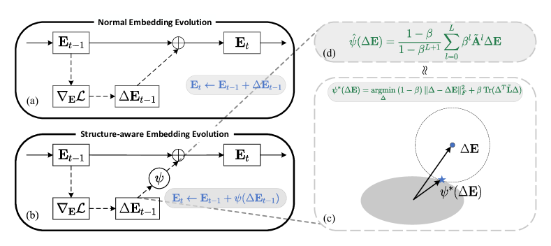
In this work, we aim to directly inject graph structure information into embedding through a novel embedding update mechanism. Figure 1 (a) illustrates a normal embedding evolution process, in which the embedding $\displaystyle\mathbf{E}$ is updated at step $\displaystyle t$ by

$$\displaystyle\mathbf{E}_{t}\leftarrow\mathbf{E}_{t-1}+\Delta\mathbf{E}_{t-1}.$$

Note that the variation $\displaystyle\Delta\mathbf{E}$ is mainly determined by the (anti-)gradient. It points to a region able to decrease a loss function concerning recommendation performance [31], but lacks an explicit guarantee that the variations between related nodes are similar. The embeddings thus cannot be expected to satisfactorily model pairwise relations while minimizing the recommendation loss.

Conversely, structure information can be learned if related nodes evolve similarly at each update. The structure-aware embedding evolution (SEvo for short), shown in Figure 1 (b), is developed for this goal. A special transformation is applied so as to meet both smoothness and convergence [48]. Because these two criteria inherently conflict to some extent, we resort to a graph regularization framework [48, 6] to balance them. While analogous frameworks have been used to understand feature smoothing and modify message passing mechanisms for GNNs [26, 51], applying this to variations is not as straightforward as to features [14] or labels [19]. Previous efforts are capable of smoothing, but cannot account for strict convergence. The specific transformation form must be chosen carefully; subtle differences may slow down or even kill training. Through an exhaustive theoretical analysis, we develop an applicable solution with a provable convergence guarantee.

Apart from the anti-gradient, the variation $\displaystyle\Delta\mathbf{E}$ can also be derived from the moment estimates. Therefore, existing optimizers, such as SGD [36] and Adam [22], can benefit from SEvo readily. In contrast to Adam, AdamW [25] decouples the weight decay from the optimization step, thereby more suitable here since it makes no sense to require the weight decay to be smooth as well. Moreover, we recorrect the moment estimates of SEvo-enhanced AdamW when encountering sparse gradients. This modification allows it to be more robust to a variety of recommendation models and scenarios. Numerous experiments over four public datasets have demonstrated that it can effectively inject structure information to boost recommendation performance. Since SEvo does not change the inference logic of the model, the inference time is exactly the same, and only negligible computational overhead is required during training.

The main contributions of this paper are summarized below.

• The graph regularization framework [48, 6] has been widely used for feature/label smoothing. To best of our knowledge, we are the first to apply it to variations as an alternative to explicit GNN modules for recommendation. The final transformation is not trivial and comes from exhaustive theoretical analyses.

• We present SEvo-enhanced AdamW by incorporating SEvo and recorrecting the original moment estimates. These modifications demonstrate consistent performance, with 7%$\displaystyle\sim$17% average improvements across a spectrum of models. Other optimizers such as SGD and Adam can be performed in a similar way with SEvo.

• We preliminarily investigate the estimation of pairwise similarity based on interaction data or prior knowledge, from which the results suggest that the utility of SEvo depends on how well the imposed structure information agrees with the performance metrics of interest. It highlights the importance of relation mining research [42].

The remainder of this paper is organized as follows. Structure-aware embedding evolution and its convergence analysis are detailed in Section 2. We then introduce in Section 3 how to integrate SEvo into existing optimizers. In addition, Section 4 provides a preliminary discussion of pairwise similarity estimation. The experiments and proofs are presented in Section 5 and Appendix, respectively.

2 structure-aware embedding evolution

In this section, we first introduce some necessary terminology and concepts, in particular smoothness. SEvo and its theoretical analyses will be detailed in Section 2.2 and 2.3. The proofs are deferred to Appendix.

2.1 Preliminaries

Notations and terminology. Let $\displaystyle\mathcal{V}=\{v_{1},\ldots,v_{n}\}$ denote a set of nodes and $\displaystyle\mathbf{A}=[w_{ij}]\in\mathbb{R}^{n\times n}$ a symmetric adjacency matrix, where each entry $\displaystyle w_{ij}=w_{ji}$ characterizes how closely $\displaystyle v_{i}$ and $\displaystyle v_{j}$ are related. They jointly constitute the graph $\displaystyle\mathcal{G}=(\mathcal{V},\mathbf{A})$. For example, $\displaystyle\mathcal{V}$ could be a set of movies, and $\displaystyle w_{ij}$ is the frequency of $\displaystyle v_{i}$ and $\displaystyle v_{j}$ being liked by the same user. Denoted by $\displaystyle\mathbf{D}\in\mathbb{R}^{n\times n}$ the diagonal degree matrix of $\displaystyle\mathbf{A}$, the normalized adjacency matrix and the corresponding Laplacian matrix are defined as $\displaystyle\tilde{\mathbf{A}}=\mathbf{D}^{-1/2}\mathbf{A}\mathbf{D}^{-1/2}$ and $\displaystyle\tilde{\mathbf{L}}=\mathbf{I}-\tilde{\mathbf{A}}$, respectively. For ease of notation, we use $\displaystyle\langle\cdot,\cdot\rangle$ to denote the inner product, $\displaystyle\langle\mathbf{x},\mathbf{y}\rangle=\mathbf{x}^{T}\mathbf{y}$ for vectors and $\displaystyle\langle\mathbf{X},\mathbf{Y}\rangle=\text{Tr}(\mathbf{X}^{T}\mathbf{Y})$ for matrices. Here, $\displaystyle\text{Tr}(\cdot)$ denotes the trace of a given matrix.

Smoothness. Before delving into the details of SEvo, it is necessary to present a metric to measure the smoothness [48, 6] of node features $\displaystyle\mathbf{X}$ as a whole. Denoted by $\displaystyle\mathbf{x}_{i},\mathbf{x}_{j}$ the row vectors of $\displaystyle\mathbf{X}$ and $\displaystyle d_{i}=\sum_{j}w_{ij}$, we have

$$\begin{array}[]{ll}\mathcal{J}_{smoothness}(\mathbf{X};\mathcal{G})&:=\text{Tr}(\mathbf{X}^{T}\tilde{\mathbf{L}}\mathbf{X})\\ &=\sum_{i,j\in\mathcal{V}}w_{ij}\bigg{\|}\frac{\mathbf{x}_{i}}{\sqrt{d_{i}}}-\frac{\mathbf{x}_{j}}{\sqrt{d_{j}}}\bigg{\|}_{2}^{2}.\end{array}$$ (1)

This term is often used as graph regularization for feature/label smoothing [14, 19]. Intuitively, a lower $\displaystyle\mathcal{J}_{smoothness}$ indicates smaller difference between closely related pairs of nodes, and in this case $\displaystyle\mathbf{X}$ is considered smoother. However, smoothness alone is not sufficient from a performance perspective. Over-emphasizing this indicator instead leads to the well-known over-smoothing issue [24]. How to balance variation smoothness and convergence is the main challenge to be addressed below.

2.2 Methodology

The entities involved in a recommender system are typically embedded into a latent space [5, 12], and the embeddings in $\displaystyle\mathbf{E}\in\mathbb{R}^{n\times d}$ are expected to be smooth so that related nodes are close to each other. In general, $\displaystyle\mathbf{E}$ is learnable and updated at step $\displaystyle t$ by

$$\mathbf{E}_{t}\leftarrow\mathbf{E}_{t-1}+\Delta\mathbf{E}_{t-1},$$

where the variation $\displaystyle\Delta\mathbf{E}$ is mainly determined by the (anti-)gradient. For example, $\displaystyle\Delta\mathbf{E}=-\eta\nabla_{\mathbf{E}}\mathcal{L}$ when gradient descent with a learning rate of $\displaystyle\eta$ is used to minimize a loss function $\displaystyle\mathcal{L}$. However, the final embeddings based on this evolution process may be far from sufficient smoothness because: 1) The variation $\displaystyle\Delta\mathbf{E}$ points to the region able to decrease the loss function concerning recommendation performance, but lacks an explicit smoothness guarantee. 2) The variations of two related nodes may be quite different due to the randomness from initialization and mini-batch sampling.

We are to design a special transformation $\displaystyle\psi(\cdot)$ to smooth the variation so that the evolution deduced from the following update formula is structure-aware,

$$\displaystyle\mathbf{E}_{t}\leftarrow\mathbf{E}_{t-1}+\psi(\Delta\mathbf{E}_{t-1}).$$ (2)

Recall that, in this paper, the similarity is confined to quantifiable values in the adjacency matrix $\displaystyle\mathbf{A}$, in which more related pairs are weighted higher. Therefore, this transformation should encourage pairs of nodes connected with higher weights to evolve more similarly than those connected with lower weights. This can be boiled down to structure-aware transformation as defined below.

Definition 1 (Structure-aware transformation).

The transformation $\displaystyle\psi(\cdot)$ is structure-aware if

$$\displaystyle\mathcal{J}_{smoothness}(\psi(\Delta\mathbf{E}))\leq\mathcal{J}_{smoothness}(\Delta\mathbf{E}).$$ (3)

On the other hand, this transformation must ensure convergence throughout the evoluton process, which means that the transformed variation should not differ too much from the original. For the sake of theoretical analysis, the ability to maintain the update direction will be used to qualitatively depict this desirable property below, though a quantitative squared error will be employed later.

Definition 2 (Direction-aware transformation).

The transformation $\displaystyle\psi(\cdot)$ is direction-aware if

$$\displaystyle\big{\langle}\psi(\Delta\mathbf{E}),\Delta\mathbf{E}\big{\rangle}>0,\quad\forall\>\Delta\mathbf{E}\not=\bm{0}.$$ (4)

These two criteria inherently conflict to some extent. We resort to a hyperparameter $\displaystyle\beta\in[0,1)$ to make a trade-off and the desired transformation is the corresponding minimum; that is ($\displaystyle\|\cdot\|_{F}$ denotes the the Frobenius norm),

$$\displaystyle\psi^{*}(\Delta\mathbf{E})=\mathop{\text{argmin}}\limits_{\Delta}\>(1-\beta)\>\|\Delta-\Delta\mathbf{E}\|_{F}^{2}+\beta\>\underbrace{\text{Tr}(\Delta^{T}\tilde{\mathbf{L}}\Delta)}_{\mathcal{J}_{smoothness}}.$$ (5)

A larger $\displaystyle\beta$ indicates a stronger smoothness constraint and $\displaystyle\psi^{*}(\Delta\mathbf{E})$ reduces to $\displaystyle\Delta\mathbf{E}$ when $\displaystyle\beta\rightarrow 0$. Geometrically, as shown in Figure 1 (c), $\displaystyle\psi^{*}(\Delta\mathbf{E})$ can be understood as a projection of $\displaystyle\Delta\mathbf{E}$ onto the region with proper smoothness. Taking the gradient to zero gives a closed-form solution:

$$\displaystyle\psi^{*}(\Delta\mathbf{E})=(1-\beta)(I-\beta\tilde{\mathbf{A}})^{-1}\Delta\mathbf{E}.$$

However, exact matrix inversion requires $\displaystyle\mathcal{O}(|\mathcal{V}|^{3})$ arithmetic operations and $\displaystyle\mathcal{O}(|\mathcal{V}|^{3})$ memory overhead, which is prohibitively expensive in recommendation due to the large number of entities. Zhou et al. [48] suggested a $\displaystyle L$-layer iterative approximation to circumvent this problem:

$$\displaystyle\hat{\psi}_{iter}(\Delta\mathbf{E}):=\hat{\psi}_{L}(\Delta\mathbf{E}),$$

$$\displaystyle\hat{\psi}_{l}(\Delta\mathbf{E})=\beta\tilde{\mathbf{A}}\hat{\psi}_{l-1}(\Delta\mathbf{E})+(1-\beta)\Delta\mathbf{E},$$

$$\displaystyle\hat{\psi}_{0}(\Delta\mathbf{E})=\Delta\mathbf{E}.$$

The resulting transformation is actually a momentum update that aggregates higher-order information layer by layer. Analogous message-passing mechanisms have been used in previous GNNs such as APPNP [14] and C&S [19]. However, this commonly used approximate solution is not compatible with SEvo; sometimes, variations after the transformation may be opposite to the original direction, leading to a failure of convergence.

Theorem 1.

The iterative approximation is direction-aware for all possible normalized adjacency matrices and $\displaystyle L\geq 0$, if and only if $\displaystyle\beta<1/2$. The Neumann series approximation

$$\displaystyle\hat{\psi}_{nsa}(\Delta\mathbf{E})=(1-\beta)\sum_{l=0}^{L}\beta^{l}\tilde{\mathbf{A}}^{l}\Delta\mathbf{E},$$ (6)

is structure-aware and direction-aware for any $\displaystyle\beta\in[0,1)$.

As suggested in Theorem 1, a compromise is to restrict $\displaystyle\beta$ to $\displaystyle[0,1/2)$ for $\displaystyle\hat{\psi}_{iter}$, but this may lead to a lack of smoothness. The Neumann series approximation [34] of Eq. (6) seems to be a viable alternative; qualitatively, it satisfies both desirable properties. Nevertheless, this transformation can be further modified for faster convergence rate based on the analysis presented next.

2.3 Convergence analysis

TABLE I: Summary of different forms of transformations.

Transformation	Structure-aware	Direction-aware	Convergence rate
$\displaystyle\hat{\psi}_{iter}$	✔
$\displaystyle\hat{\psi}_{nsa}$	✔	✔	$\displaystyle\mathcal{O}\big{(}C/((1-\beta)^{2}T)\big{)}$
$\displaystyle\hat{\psi}$	✔	✔	$\displaystyle\mathcal{O}\big{(}C/((1-\beta)T)\big{)}$

In general, the recommender system has some additional parameters $\displaystyle\bm{\theta}\in\mathbb{R}^{m}$ except for embedding to be trained. Therefore, we analyze the convergence rate of the following gradient descent strategy:

$$\displaystyle\mathbf{E}_{t+1}\leftarrow\mathbf{E}_{t}-\eta\hat{\psi}_{nsa}\big{(}\nabla_{\mathbf{E}}\mathcal{L}(\mathbf{E}_{t},\bm{\theta}_{t})\big{)},$$

$$\displaystyle\bm{\theta}_{t+1}\leftarrow\bm{\theta}_{t}-\eta^{\prime}\nabla_{\bm{\theta}}\mathcal{L}(\mathbf{E}_{t},\bm{\theta}_{t}).$$

wherein SEvo is performed on the embedding and a normal gradient descent is applied to $\displaystyle\bm{\theta}$. To make the analysis feasible, some mild assumptions on the loss function should be given: $\displaystyle\mathcal{L}:\mathbb{R}^{n\times d}\times\mathbb{R}^{m}\rightarrow\mathbb{R}$ is a 2-times continuously differentiable function whose first derivative is Lipschitz continuous for some constant $\displaystyle C$. Then, we have the following properties.

Theorem 2.

If $\displaystyle\eta=\eta^{\prime}=1/C$, after $\displaystyle T$ updates, we have

$$\displaystyle\min_{t\leq T}\|\nabla\mathcal{L}(\mathbf{E}_{t},\bm{\theta}_{t})\|_{2}^{2}=\mathcal{O}\big{(}C/((1-\beta)^{2}T)\big{)}.$$

If we adopt a modified learning rate for embedding:

$$\displaystyle\eta=\frac{1}{(1-\beta^{L+1})C},$$

the convergence rate could be improved to $\displaystyle\mathcal{O}\big{(}C/((1-\beta)T)\big{)}$.

Remark 1.

Our main interest is to justify the designs of SEvo rather than to pursue a particular convergence rate, so some mild assumptions suggested in [30] are adopted here. By introducing the steepest descent for quadratic norms [1], better convergence can be obtained with stronger assumptions.

Two conclusions can be drawn from Theorem 2. 1) The theoretical upper bound becomes worse when $\displaystyle\beta\rightarrow 1$. This makes sense since $\displaystyle\hat{\psi}_{nsa}(\nabla_{\mathbf{E}}\mathcal{L})$ is getting smoother and further away from the original descent direction. 2) A modified learning rate for embedding can significantly improve the convergence rate. This phenomenon can be understood readily if we notice the fact that

$$\displaystyle\|\hat{\psi}_{nsa}(\Delta\mathbf{E})\|_{F}\leq(1-\beta^{L+1})\|\Delta\mathbf{E}\|_{F}.$$

So the modified learning rate is indeed to offset the scaling effect resulted from SEvo. In view of this, we integrate this factor into SEvo to avoid getting stuck in the learning rate search, yielding the final transformation:

$$\displaystyle\hat{\psi}(\Delta\mathbf{E})=\frac{1-\beta}{1-\beta^{L+1}}\sum_{l=0}^{L}\beta^{l}\tilde{\mathbf{A}}^{l}\Delta\mathbf{E}.$$ (7)

It can be shown that $\displaystyle\hat{\psi}$ is structure-aware and direction-aware, and still converges to $\displaystyle\psi$ when $\displaystyle L$ increases.

2.4 Time Complexity

The time complexity of SEvo is mainly determined by the arithmetic operations of $\displaystyle\tilde{\mathbf{A}}^{l}\Delta\mathbf{E},l=1,2,\ldots,L$. Assuming that the number of non-zero entries of $\displaystyle\tilde{\mathbf{A}}$ is $\displaystyle S$, the complexity required is about $\displaystyle\mathcal{O}(LSd)$. Because the recommendation datasets are known for high sparsity (i.e., $\displaystyle S$ is very small), the actual computational overhead can be reduced to a very low level, almost negligible (see Section 5.2 for an empirical verification).

3 Integrating SEvo into existing optimizers

Input: learning rate $\displaystyle\eta$, momentum factors $\displaystyle\beta_{1},\beta_{2},\beta\in[0,1)$, weight decay $\displaystyle\lambda$.

foreach step $\displaystyle t$ do

      

      $\displaystyle\mathbf{G}_{t}\leftarrow\nabla_{\mathbf{E}}\mathcal{L}$ ;

        // Get gradients w.r.t $\displaystyle\mathbf{E}$

      

      foreach node $\displaystyle i$ do

            

            

$$\displaystyle\mathbf{M}_{t}[i]\leftarrow\left\{\begin{array}[]{ll}\beta_{1}\mathbf{M}_{t-1}[i]+(1-\beta_{1})\mathbf{G}_{t}[i]&\text{ if }\mathbf{G}_{t}[i]\not=\bm{0}\\ \beta_{1}\mathbf{M}_{t-1}[i]+(1-\beta_{1})\frac{1}{1-\beta_{1}^{t-1}}\mathbf{M}_{t-1}[i]&\text{ otherwise }\end{array}\right.,$$

$$\displaystyle\mathbf{V}_{t}[i]\leftarrow\left\{\begin{array}[]{ll}\beta_{1}\mathbf{V}_{t-1}[i]+(1-\beta_{2})\mathbf{G}_{t}^{2}[i]&\text{ if }\mathbf{G}_{t}[i]\not=\bm{0}\\ \beta_{1}\mathbf{V}_{t-1}[i]+(1-\beta_{2})\frac{1}{1-\beta_{2}^{t-1}}\mathbf{V}_{t-1}[i]&\text{ otherwise }\end{array}\right.;$$

      

      Compute bias-corrected first and second moment estimates:

$$\displaystyle\hat{\mathbf{M}}_{t}\leftarrow\mathbf{M}_{t}/(1-\beta_{1}^{t}),\quad\hat{\mathbf{V}}_{t}\leftarrow\mathbf{V}_{t}/(1-\beta_{2}^{t});$$

      Update via SEvo:

$$\displaystyle\mathbf{E}_{t}\leftarrow\mathbf{E}_{t-1}-\eta\>\hat{\psi}\bigg{(}\hat{\mathbf{M}}_{t}/\sqrt{\hat{\mathbf{V}}_{t}+\epsilon};\beta\bigg{)}-\eta\lambda\mathbf{E}_{t-1}.$$

Output: optimized embeddings $\displaystyle\mathbf{E}$.

Algorithm 1 AdamW enhanced by SEvo. We omit the details regarding the other parameters as they are identical to AdamW. The matrix operations below are element-wise.

Input: learning rate $\displaystyle\eta$, momentum factors $\displaystyle\mu,\beta\in[0,1)$, weight decay $\displaystyle\lambda$.

foreach step $\displaystyle t$ do

      

      $\displaystyle\mathbf{G}_{t}\leftarrow\nabla_{\mathbf{E}}\mathcal{L}+\lambda\mathbf{E}_{t-1}$ ;

        // Get gradients

       $\displaystyle\mathbf{M}_{t}\leftarrow\mu\mathbf{M}_{t-1}+\mathbf{G}_{t}$ ;

        // Moment update

      

      Update via SEvo:

$$\displaystyle\mathbf{E}_{t}\leftarrow\mathbf{E}_{t-1}-\eta\>\hat{\psi}\bigg{(}\mathbf{M}_{t};\beta\bigg{)}.$$

Output: optimized embeddings $\displaystyle\mathbf{E}$.

Algorithm 2 SGD with momentum enhanced by SEvo. We omit the details regarding the other parameters as they are identical to SGD. The matrix operations below are element-wise.

Input: learning rate $\displaystyle\eta$, momentum factors $\displaystyle\beta_{1},\beta_{2},\beta\in[0,1)$, weight decay $\displaystyle\lambda$.

foreach step $\displaystyle t$ do

      

      $\displaystyle\mathbf{G}_{t}\leftarrow\nabla_{\mathbf{E}}\mathcal{L}+\lambda\mathbf{E}_{t-1}$ ;

        // Get gradients

      

      Update first/second moment estimates:

$$\displaystyle\mathbf{M}_{t}\leftarrow\beta_{1}\mathbf{M}_{t-1}+(1-\beta_{1})\mathbf{G}_{t},$$

$$\displaystyle\quad\mathbf{V}_{t}\leftarrow\beta_{1}\mathbf{V}_{t-1}+(1-\beta_{2})\mathbf{G}_{t}^{2};$$

      Compute bias-corrected first and second moment estimates:

$$\displaystyle\hat{\mathbf{M}}_{t}\leftarrow\mathbf{M}_{t}/(1-\beta_{1}^{t}),$$

$$\displaystyle\quad\hat{\mathbf{V}}_{t}\leftarrow\mathbf{V}_{t}/(1-\beta_{2}^{t});$$

      Update via SEvo:

$$\displaystyle\mathbf{E}_{t}\leftarrow\mathbf{E}_{t-1}-\eta\>\hat{\psi}\bigg{(}\hat{\mathbf{M}}_{t}/\sqrt{\hat{\mathbf{V}}_{t}+\epsilon};\beta\bigg{)}.$$

Output: optimized embeddings $\displaystyle\mathbf{E}$.

Algorithm 3 Adam with momentum enhanced by SEvo. We omit the details regarding the other parameters as they are identical to Adam. The matrix operations below are element-wise.

SEvo can be seamlessly integrated into existing optimizers since the variation involved in Eq. (2) can be extended beyond the (anti-)gradient. For SGD with momentum, the variation becomes the first-moment estimate, and for Adam, this is jointly determined by the first/second-moment estimates. AdamW is also widely adopted for training recommenders. Unlike Adam whose moment estimate is a mixture of gradient and weight decay, AdamW decouples the weight decay from the optimization step, which is preferable since it makes no sense to require the weight decay to be smooth as well. However, in very rare cases (see Section 5.5), SEvo-enhanced AdamW fails to work. We next try to ascertain the causes and then propose a modification to make SEvo-enhanced AdamW more robust. The algorithms of these SEvo-enhanced optimizers are respectively summarized as Algorithm 2, 3, and 1. An empirical comparison can be found in Section 5.2.

Denoted by $\displaystyle\mathbf{g}:=\nabla_{\mathbf{e}}\mathcal{L}\in\mathbb{R}^{d}$ the gradient for a node embedding $\displaystyle\mathbf{e}$ and $\displaystyle\mathbf{g}^{2}:=\mathbf{g}\odot\mathbf{g}$ the element-wise square, AdamW estimates the first and second moments at step $\displaystyle t$ by the following formulas

$$\displaystyle\mathbf{m}_{t}=\beta_{1}\mathbf{m}_{t-1}+(1-\beta_{1})\mathbf{g}_{t-1},$$

$$\displaystyle\mathbf{v}_{t}=\beta_{2}\mathbf{v}_{t-1}+(1-\beta_{2})\mathbf{g}_{t-1}^{2},$$

where $\displaystyle\beta_{1},\beta_{2}$ are the momentum factors. The resulting update mechanism for each embedding is

$$\displaystyle\mathbf{e}_{t}=\mathbf{e}_{t-1}-\eta\cdot\Delta\mathbf{e}_{t-1},\quad\Delta\mathbf{e}_{t-1}:=\hat{\mathbf{m}}_{t}/\sqrt{\hat{\mathbf{v}}_{t}}.$$

Note that the bias-corrected estimates $\displaystyle\hat{\mathbf{m}}_{t}=\mathbf{m}_{t}/(1-\beta_{1}^{t})$ and $\displaystyle\hat{\mathbf{v}}_{t}=\mathbf{v}_{t}/(1-\beta_{2}^{t})$ are employed here for numerical stability [22]. In practice, only a fraction of nodes will be sampled for training in a mini-batch, so the remaining embeddings have zero gradients. In this case, the sparse gradient problem may cause some unexpected ‘biases’.

Proposition 1.

If the node is no longer sampled in subsequent $\displaystyle p$ batches after step $\displaystyle t$, we have

$$\displaystyle\Delta\mathbf{e}_{t+p-1}=\kappa\cdot\frac{\beta_{1}^{p}}{\sqrt{\beta_{2}^{p}}}\Delta\mathbf{e}_{t-1},$$ (8)

where the coefficient of $\displaystyle\kappa$ is mainly determined by $\displaystyle t$.

For a common case $\displaystyle\beta_{2}\approx\beta_{1}$, the right-hand side of Eq. (8) is close to $\displaystyle\mathcal{O}(\beta_{1}^{p/2})$. The step size for inactive nodes gets slower and slower during idle periods. This appears reasonable as their moment estimates are becoming outdated; however, this effect sometimes prevents the variation from being smoothed by SEvo. We hypothesize that this is because SEvo itself tends to assign more energy to active nodes and less energy to inactive nodes. So the effect of Eq. (8) is somewhat redundant. Fortunately, there is a feasible modification to make SEvo-enhanced AdamW more robust:

Theorem 3.

Under the same assumptions as in Proposition 1, $\displaystyle\Delta\mathbf{e}_{t+p-1}=\Delta\mathbf{e}_{t-1}$ if the moment estimates are updated in the following manner when $\displaystyle\mathbf{g}_{t}=\bm{0}$,

$$\displaystyle\mathbf{m}_{t}=\beta_{1}\mathbf{m}_{t-1}+(1-\beta_{1})\frac{1}{1-\beta_{1}^{t-1}}\mathbf{m}_{t-1},$$ (9)

$$\displaystyle\mathbf{v}_{t}=\beta_{2}\mathbf{v}_{t-1}+(1-\beta_{2})\frac{1}{1-\beta_{2}^{t-1}}\mathbf{v}_{t-1}.$$ (10)

As can be seen, when sparse gradients are encountered, the approach in Theorem 3 is actually to estimate the current gradient from previous moments. The coefficients $\displaystyle 1/(1-\beta_{1}^{t-1})$ and $\displaystyle 1/(1-\beta_{1}^{t-1})$ are used here for unbiasedness (refer to Appendix LABEL:section-proof-loce-enhanced-Adamw for detailed discussion and proof).

4 Pairwise similarity estimation

Figure 2: Illustrations of different pairwise similarity estimation methods based on interaction data. (a) The default is to adopt the co-occurrence frequency within the last $\displaystyle K$ items. (b) Using only the first $\displaystyle K$ items. (c) Allowing a maximum path length of $\displaystyle H$ beyond 1. (d) Frequency-based similarity versus distance-based similarity.

⬇

for seq in seqs:

if first:

seq = seq[:K] # First K items

else:

seq = seq[-K:] # Last K items

for i in range(len(seq) - 1):

for h, j in enumerate( # Maximum path length H

range(i + 1, min(i + H + 1, len(seq))),

start=1

):

if frequency: # Frequency

A[seq[i], seq[j]] += 1

A[seq[j], seq[i]] += 1

else: # Distance

A[seq[i], seq[j]] += 1 / h

A[seq[j], seq[i]] += 1 / h

Algorithm 4 Python-style algorithm for similarity estimation based on interaction data.

Here, we preliminarily explore some of the factors that may impact similarity estimation; more empirical comparisons can be found in Section 5.6. Note that the following attempts focus on the intrinsic nature of datasets, e.g., preferences and genres. A more comprehensive study regarding graph construction [20] (e.g., sparsification and reweighting) is beyond the scope of this paper. We leave it as a future work.

Pairwise similarity based on interaction data. Recent GNN-based sequence models [43, 44], as well as the SEvo-enhanced models in Section 5, estimate the pairwise similarity $\displaystyle w_{ij}$ between items $\displaystyle v_{i}$ and $\displaystyle v_{j}$ based on their co-occurrence frequency in sequences. In other words, items that appear consecutively more often are assumed more related. There are some factors that deserve a closer look:

• The maximum sequence length $\displaystyle K$ for construction to investigate the number of interactions required for accurate estimation.

• Using only the first $\displaystyle K$ versus last $\displaystyle K$ interactions in each sequence to compare the utility of early and recent preferences.

• Allowing related items to be connected by a path of length $\displaystyle\leq H$ rather than strict consecutive occurrences.

• Frequency-based similarity versus distance-based similarity. The former weights all related pairs equally, while the latter weights inversely to their path length. For example, given a sequence $\displaystyle v_{2}\rightarrow v_{1}\rightarrow v_{3}$ with a maximum path length of $\displaystyle H=2$, the frequency-based similarity of $\displaystyle(v_{2},v_{3})$ gives 1, while the distance-based similarity is $\displaystyle 1/2$ (as the path length from $\displaystyle v_{2}$ to $\displaystyle v_{3}$ is $\displaystyle 2$).

Figure 2 illustrates these four variants and Algorithm 4 details a step-by-step process.

Pairwise similarity based on prior knowledge. Sometimes embeddings are expected to be smooth w.r.t. a prior knowledge. For example, in addition to the interaction data, each movie in the MovieLens-1M dataset is associated with at least one genre. It is natural to assume that movies of the same genre are related to each other. Heuristically, we can define the similarity $\displaystyle w_{ij}$ to be 1 if $\displaystyle v_{i}$ and $\displaystyle v_{j}$ belong to the same genre and 0 otherwise.

TABLE II: Dataset statistics

Dataset	#Users	#Items	#Interactions	Density	Avg. Length
Beauty	22,363	12,101	198,502	0.07%	8.9
Toys	19,412	11,924	167,597	0.07%	8.6
Tools	16,638	10,217	134,476	0.08%	8.1
MovieLens-1M	6,040	3,416	999,611	4.84%	165.5

TABLE III: Overall performance comparison. The best baselines and ours are underlined and bolded, respectively. Symbol $\displaystyle\blacktriangle$% stands for the relative improvement between them. Paired t-test is performed over 5 independent runs for evaluating $\displaystyle p$-value ($\displaystyle\leq 0.05$ indicates statistical significance). ‘Avg. Improv.’ for each backbone depicts average relative improvements against the baseline. ‘U-I’ indicates using SEvo-enhanced AdamW with the user-item bipartite graph while ‘I-I’ with the item-item graph.

		GNN-based				MF or RNN/Transformer-based											$\displaystyle\blacktriangle$%	p-value
		LightGCN	SR-GNN	LESSR	MAERec	MF-BPR			GRU4Rec		SASRec		BERT4Rec		STOSA
							U-I	I-I		I-I		I-I		I-I		I-I
Beauty	HR@1	0.0074	0.0059	0.0088	0.0113	0.0071	0.0071	0.0076	0.0061	0.0094	0.0120	0.0154	0.0157	0.0172	0.0166	0.0216	30.2%	6.90E-05
	HR@5	0.0289	0.0247	0.0322	0.0424	0.0272	0.0281	0.0293	0.0233	0.0326	0.0404	0.0499	0.0479	0.0522	0.0479	0.0544	13.5%	7.69E-04
	HR@10	0.0472	0.0406	0.0506	0.0662	0.0454	0.0461	0.0480	0.0395	0.0524	0.0634	0.0759	0.0716	0.0772	0.0680	0.0774	8.2%	2.66E-03
	NDCG@5	0.0181	0.0152	0.0205	0.0269	0.0170	0.0175	0.0184	0.0146	0.0209	0.0262	0.0328	0.0319	0.0350	0.0327	0.0383	17.2%	9.70E-05
	NDCG@10	0.0240	0.0203	0.0264	0.0346	0.0228	0.0233	0.0244	0.0198	0.0273	0.0336	0.0411	0.0395	0.0430	0.0391	0.0457	15.5%	8.02E-05
Toys	HR@1	0.0087	0.0100	0.0126	0.0171	0.0079	0.0084	0.0099	0.0059	0.0080	0.0172	0.0192	0.0160	0.0175	0.0232	0.0267	15.3%	1.46E-03
	HR@5	0.0279	0.0294	0.0352	0.0532	0.0267	0.0288	0.0306	0.0209	0.0276	0.0506	0.0584	0.0430	0.0492	0.0571	0.0625	9.6%	5.70E-03
	HR@10	0.0456	0.0439	0.0513	0.0796	0.0427	0.0447	0.0477	0.0345	0.0446	0.0727	0.0844	0.0645	0.0723	0.0776	0.0872	9.5%	3.07E-04
	NDCG@5	0.0183	0.0198	0.0240	0.0355	0.0174	0.0187	0.0203	0.0134	0.0179	0.0342	0.0392	0.0297	0.0336	0.0406	0.0453	11.6%	2.48E-03
	NDCG@10	0.0240	0.0245	0.0292	0.0440	0.0225	0.0238	0.0258	0.0177	0.0234	0.0413	0.0475	0.0366	0.0410	0.0472	0.0532	12.7%	3.12E-05
Tools	HR@1	0.0067	0.0046	0.0045	0.0083	0.0058	0.0068	0.0071	0.0053	0.0058	0.0099	0.0108	0.0074	0.0087	0.0095	0.0133	33.8%	1.23E-02
	HR@5	0.0212	0.0162	0.0157	0.0271	0.0187	0.0216	0.0225	0.0174	0.0208	0.0317	0.0337	0.0244	0.0279	0.0276	0.0350	10.5%	8.94E-03
	HR@10	0.0326	0.0260	0.0263	0.0423	0.0293	0.0342	0.0348	0.0272	0.0336	0.0466	0.0497	0.0405	0.0441	0.0417	0.0502	7.7%	8.25E-03
	NDCG@5	0.0140	0.0103	0.0101	0.0177	0.0123	0.0142	0.0147	0.0114	0.0133	0.0210	0.0223	0.0159	0.0183	0.0186	0.0244	15.9%	5.57E-03
	NDCG@10	0.0176	0.0135	0.0135	0.0226	0.0157	0.0182	0.0187	0.0145	0.0174	0.0258	0.0274	0.0211	0.0235	0.0231	0.0293	13.4%	3.79E-03
MovieLens	HR@1	0.0124	0.0383	0.0513	0.0439	0.0117	0.0125	0.0133	0.0487	0.0487	0.0490	0.0517	0.0681	0.0733	0.0457	0.0510	7.6%	3.81E-02
	HR@5	0.0495	0.1297	0.1665	0.1563	0.0470	0.0501	0.0509	0.1625	0.1663	0.1599	0.1670	0.2069	0.2127	0.1409	0.1569	2.8%	4.17E-03
	HR@10	0.0866	0.2009	0.2539	0.2462	0.0836	0.0868	0.0876	0.2522	0.2568	0.2492	0.2567	0.3018	0.3075	0.2185	0.2356	1.9%	9.32E-02
	NDCG@5	0.0307	0.0842	0.1092	0.1003	0.0291	0.0313	0.0319	0.1061	0.1075	0.1046	0.1096	0.1387	0.1437	0.0932	0.1041	3.6%	4.19E-04
	NDCG@10	0.0427	0.1071	0.1373	0.1292	0.0408	0.0430	0.0436	0.1350	0.1366	0.1333	0.1385	0.1693	0.1743	0.1181	0.1295	2.9%	1.30E-02
Avg. Improv.							+7.6%	+13.1%		+23.4%		+12.3%		+9.6%		+17.5%

Figure 3: Training and inference efficiency comparisons. The wall time (seconds) is evaluated on an Intel Xeon E5- 2620 v4 platform and a single GTX 1080Ti GPU. The bars are drawn in the same order as in Table III, and the original and SEvo-enhanced models are represented by a pair of bars ‘’.

5 Experiments

In this section, we comprehensively verify the superiority of SEvo. We focus on sequential recommendation for two reasons: 1) This is the most common scenario in practice; 2) Utilizing both sequence and structure information is beneficial yet challenging. We wish to show that structure-aware embedding evolution is a promising way to achieve this goal.

The remainder of this section is organized as follows. Firstly, an overall comparison is reported in Section 5.2. The empirical results in Section 5.3 then verify previous statements, showing both convergence and smoothness performance throughout training. An exhaustive ablation study will be given in Section 5.4. We also demonstrate in Section 5.5 the correction of SEvo-enhanced AdamW. Finally, Section 5.6 investigates the four factors in terms of similarity estimation.

5.1 Experimental Setup

This part introduces the datasets, evaluation metrics, baselines, and implementation details.

(a) Loss curves

(b) Smoothness

Figure 4: Empirical illustrations of convergence and smoothness. The top and bottom panels respectively depict the results for Beauty and MovieLens-1M. (a) SASRec enhanced by SEvo with or without rescaling. (b) Smoothness of (I) the original variation; (II) the smoothed variation; (III) the optimized embedding. A lower $\displaystyle\mathcal{J}_{smoothness}$ indicates stronger smoothness.

Datasets. Four benchmark datasets, including Beauty, Toys, Tools, and MovieLens-1M, are considered in this paper. The first three are e-commerce datasets from Amazon reviews known for high sparsity, and MovieLens-1M is a movie dataset with a much longer sequence length. Following [21, 13], we filter out users and items with less than 5 interactions, and the validation set and test set are split in a leave-one-out fashion, namely the last interaction for testing and the penultimate one for validation. This splitting allows for fair comparisons, either for sequential recommendation or collaborative filtering. The dataset statistics are presented in Table II.

Evaluation metrics. For each user, the predicted scores returned by the recommender will be sorted in ascending order to generate top-N candidate lists. We consider two widely-used evaluation metrics, HR@N (Hit Rate) and NDCG@N (Normalized Discounted Cumulative Gain). The former measures the rate of successful hits among the top-N recommended candidates, while the latter takes into account the ranking positions and assigns higher scores in order of priority.

Baselines. Firstly, four GNN-based models are considered here as benchmarks for performance and efficiency comparisons. We carefully tune the hyperparameters according to their open-source code and experimental settings.

• LightGCN [17] is a pioneering collaborative filtering model that simplifies graph convolutional networks (GCNs) by removing nonlinearities for easier training. It uses only graph structure information and has no access to sequence information.

• SR-GNN [43] and LESSR [7] are two baselines dynamically constructing session graph. The former employs a gated graph neural network to obtain the final node vectors, while the latter utilizes edge-order preserving multigraph and a shortcut graph to address the lossy session encoding and ineffective long-range dependency capturing problems, respectively.

• MAERec [45] learns to sample less noisy paths from a semantic similarity graph for subsequent reconstruction tasks. However, we found that the official implementation treats the recommendation loss and reconstruction loss equally, leading to poor performance here. Therefore, an additional weight is attached to the reconstruction loss and a grid search is performed in the range of [0, 1]. Almost all hyperparameters are tuned for competitive performance.

In order to investigate the effectiveness of SEvo, four sequence models, GRU4Rec, SASRec, BERT4Rec and STOSA are selected as the backbones. They cover RNN/Transformer-based architectures and various self-attention mechanisms:

• GRU4Rec [18] applies RNN [9] to recommendation with specific modifications made to cope with data sparsity. In addition to the learning rate in {1e-4, 5e-4, 1e-3, 5e-3} and weight decay in [0, 0.1], we also tune the dropout rate for node features in the range of [0, 0.7].

• SASRec [21] and BERT4Rec [35] are two pioneering works on sequential recommendation equipped with unidirectional and bidirectional self-attention, respectively. For BERT4Rec which employs a separate fully-connected layer for scoring, the weight matrix therein will also be smoothed by SEvo. In addition to some basic hyperparameters, the mask ratio is also researched for BERT4Rec.

• STOSA [13] is one of the state-of-the-art models. It aims to capture the uncertainty of sequential behaviors by modeling each item as a Gaussian distribution. The hyperparameters involved are tuned similarly to SASRec.

Besides, MF-BPR [31] is also considered here as a backbone without sequence modeling.

Implementation details. Since the purpose is to study the effectiveness of SEvo, only hyperparameters concerning optimization are researched, including learning rate, weight decay and dropout rate. Other hyperparameters in terms of the architecture are consistent with the corresponding baseline. For a fair comparison, the number of layers $\displaystyle L$ is fixed to 3 as in other GNN-based recommenders. As for the hyperparameter in terms of the degree of smoothness, $\displaystyle\beta=0.99$ performs quite well in practice.

5.2 Overall comparison

In this section, we are to verify the effectiveness of SEvo in boosting recommendation performance. Table III and Figure 3 respectively compare the overall performance and efficiency over four public datasets, from which we have the following key observations:

• GNN-based models seem to over-emphasize structure information but lack full exploitation of sequence information. Their performance is only on par with GRU4Rec, a simple RNN with only one GRU layer. On the Tools dataset, SR-GNN and LESSR are even inferior to LightGCN, a collaborative filtering model with no access to sequence information. MAERec makes a slightly better attempt to combine the two by learning structure information through graph-based reconstruction tasks. It employs a SASRec backbone for recommendation to allow for a better utilization of sequence information. However, either dynamic graph construction in SR-GNN and LESSR, or path sampling in MAERec, requires heavy computational overhead. Particularly for SR-GNN and LESSR, these expensive costs are inevitable in both training and inference. Thus, previous efforts in mining graph structure information probably conflict with sequence information and are difficult to scale.

• Due to Transformer’s impressive capability in sequence encoding, SASRec, BERT4Rec and STOSA all achieve superior performance compared to GNN-based counterparts. Structure information learned through SEvo remains instrumental even for state-of-the-art models, providing consistent performance gains of 2% to 30%. Moreover, SASRec trained with SEvo-enhanced AdamW has outperformed MAERec despite their identical recommendation backbones. Note that SEvo does not change the inference logic of the model, so the inference time is exactly the same. The computational overhead required in training is also negligible compared to previous graph-enhanced models that employ GNNs as intermediate modules. SEvo is arguably superior to these cumbersome GNN modules in real-world applications. Overall, the significant improvements from the SEvo enhancement suggest a promising route to exploit both sequence and graph structure information.

• Non-sequential models such as MF-BPR can also benefit from SEvo. In addition to the item-item (I-I) graph, Table III also reports the performance with the user-item (U-I) bipartite graph. As suggested in LightGCN, the entry $\displaystyle w_{ij}=1$ if user $\displaystyle i$ has interacted with item $\displaystyle j$ before and $\displaystyle w_{ij}=0$ otherwise. On the one hand, MF-BPR enhanced by SEvo achieves comparable performance to LightGCN, demonstrating the universality of SEvo. On the other hand, the slightly superior performance of the I-I graph implies that modeling pairwise relations solely based on interactions may be too coarse. We further discuss the importance of similarity estimation in Section 5.6.

Since SASRec is a pioneer in the field of sequential recommendation, it will serve as the default backbone for the subsequent study of SEvo.

5.3 Empirical analysis

Convergence comparison. In Section 2.3, we theoretically verified the necessity of rescaling the original Neumann series approximation for faster convergence. Figure 4a shows the loss curves of SASRec trained with AdamW using identical settings other than the form of SEvo. Without rescaling, SASRec exhibits significantly slower convergence, consistent with the conclusion in Theorem 2. While the theoretical worst-case convergence rate of the corrected SEvo is only 1% of the normal gradient descent when $\displaystyle\beta=0.99$, its practical performance is much better. SASRec trained with SEvo-enhanced AdamW initially converges marginally slower and catches up in the final stage.

Smoothness evaluation. Figure 4b demonstrates the variation’s smoothness throughout the evolution process and the embedding differences from $\displaystyle\beta=0$ to $\displaystyle\beta=0.999$. (I) $\displaystyle\rightarrow$ (II): The original variations are roughly as smooth, but after transformation, they are quite different—–smoother as $\displaystyle\beta$ increases. (II) $\displaystyle\rightarrow$ (III): Consequently, the embedding trained with a stronger smoothness constraint becomes smoother as well. The structure-aware embedding evolution successfully makes related nodes closer in the latent space. Although smoothness is not the sole quality measure of embedding, combined with the analyses above, we can conclude that SEvo injects appropriate structure information under the default setting of $\displaystyle\beta=0.99$.

(a) SEvo for various optimizers

(b) SEvo using different approximations

Figure 5: SEvo ablation experiments: (a) SEvo-enhanced SGD, Adam and AdamW; (b) Neumann series approximation versus iterative approximation.

TABLE IV: SEvo using different approximation layers $\displaystyle L$.

	Beauty			MovieLens1M
	HR@1	HR@10	NDCG@10	HR@1	HR@10	NDCG@10
L=0	0.0124	0.0664	0.0353	0.0465	0.2487	0.1321
L=1	0.0140	0.0717	0.0388	0.0498	0.2562	0.1372
L=2	0.0152	0.0740	0.0403	0.0511	0.2589	0.1389
L=3	0.0154	0.0759	0.0411	0.0517	0.2567	0.1385
L=4	0.0153	0.0755	0.0408	0.0510	0.2576	0.1383
L=5	0.0150	0.0750	0.0403	0.0492	0.2581	0.1382

5.4 Ablation study

SEvo for various optimizers. It is of interest to study whether SEvo can be extended to other commonly used optimizers such as SGD and Adam. Figure 5a compares NDCG@10 performance on Beauty and MovieLens-1M. For a fair comparison, the hyperparameters are tuned independently. It is clear that the SEvo-enhanced optimizers enjoy superior performance gains on both datasets.

Neumann series approximation versus iterative approximation. Theorem 1 suggests that the Neumann series approximation is preferable to the iterative approximation because the latter is not always direction-aware and thus a conservative hyperparameter of $\displaystyle\beta$ is needed to ensure convergence. This conclusion can also be drawn from Figure 5b. When a little smoothness is required, their performance is comparable as both approximations differ only at the last term. The iterative approximation however fails to ensure convergence once $\displaystyle\beta>0.7$ on Beauty and $\displaystyle\beta>0.9$ on MovieLens-1M. This may result in a lack of smoothness.

$\displaystyle L$-layer Approximation. As $\displaystyle L$ increases, SEvo gets closer to the exact solution while accessing higher-order neighborhood information. Table IV lists the performance of different layers, which reaches its peak around $\displaystyle L=3$ and starts to decrease then. A possible reason is that the higher-order information is not as reliable and easy to use as the lower order information.

5.5 Moment estimate correction for AdamW

Figure 6: Performance comparison of SEvo-enhanced AdamW with or without moment estimate correction. ‘Avg. Improv.’ for each backbone depicts the average relative improvements against the baseline across all datasets and metrics.

We compare SEvo-enhanced AdamW with or without moment estimate correction in Figure 6, in which average relative improvements against the baseline are presented for each recommender. Overall, the two variants of SEvo-enhanced AdamW perform comparably, significantly surpassing the baseline. However, in some cases (e.g., GRU4Rec and STOSA), the moment estimate correction as suggested in Theorem 3 is particularly useful to improve performance. Recall that BERT4Rec is trained using the output softmax from a separate fully-connected layer that is fully updated at each step. This may explain why the correction has little effect on BERTRec. In conclusion, the results highlight the importance of the proposed modification in alleviating bias in moment estimates.

5.6 Pairwise similarity estimation

(a) Sequence length

(b) Frequency-based versus Distance-based

Figure 7: Comparison of similarity estimation across four potential factors. ‘$\displaystyle\star$’ indicates the default way applied to SEvo-enhanced sequence models in Section 5.2. (a) Using only the first/last $\displaystyle K$ items for pairwise similarity estimation. (b) Frequency- and distance-based similarity with a maximum path length of $\displaystyle H$.

Pairwise similarity based on interaction data. We empirically compare four potential factors in Figure 7:

• Figure 7a shows the effect of limiting the maximum sequence length to the first/last $\displaystyle K$ items, so only the early/recent preferences will be considered. In constrast to early interactions, recent ones imply more precise pairwise relations for future prediction, even for small $\displaystyle K$. With the increasing of the maximum sequence length, the recommendation performance on Beauty increases steadily, but not the case for MovieLens-1M. This suggests that shopping relations may be more consistent than movie preferences. The latter may be more diverse among different users. Excessively long sequences cause the similarity estimation to be skewed toward the tastes of mass viewing users.

• Figure 7b explores the relations beyond strict consecutive occurrences; that is, two items are considered related once they co-occur within a path of length $\displaystyle\leq H$. For the shopping and movie datasets, estimating similarity beyond co-occurrence frequency appears less reliable overall. We also compare frequency-based similarity with distance-based similarity that decreases weights for more distant pairs. It is clear that the distance-based approach performs more stable as the maximum path length $\displaystyle H$ increases.

Figure 8: UMAP [28] visualization of movies based on their embeddings. For ease of differentiation, we group the 18 genres into 6 categories and colored them individually: Thriller/Crime/Action/Adventure; Horror/Mystery/Film-Noir; War/Drama/Romance; Comedy/Musical/Children’s/Animation; Fantasy/Sci-Fi; Western/Documentary.

TABLE V: Pairwise similarity estimation based on interaction data versus prior knowledge (movie genres).

		MovieLens-1M
	$\displaystyle\beta$	HR@1	HR@10	NDCG@10
Baseline	0	0.0457	0.2482	0.1315
Interaction data	0.5	0.0494	0.2538	0.1362
	0.99	0.0517	0.2567	0.1385
Prior knowledge	0.5	0.0492	0.2527	0.1352
	0.99	0.0508	0.2549	0.1371

Pairwise similarity based on prior knowledge. Each movie in the MovieLens-1M dataset is associated with at least one genre and it is natural to assume that movies of the same genre are related to each other. As can be seen in Figure 8, such smoothness constraint can also be fulfilled through SEvo, leading to progressively stronger clustering effects as $\displaystyle\beta$ increases. However, the resulting performance gains are slightly less than those based on interaction data (see Table V). One possible reason is that the viewing order is interest rather than genre oriented, and the movie genres are too coarse to provide particularly useful information. In conclusion, while smoothness is an appealing inductive bias, its utility depends on how well the imposed structure information agrees with the performance metrics of interest.

6 Related work

Recommender systems are developed to enable users to quickly and accurately find relevant items in diverse applications, such as e-commerce [49], online news [16] and social media [4]. Typically, the entities involved are embedded into a latent space [5, 12, 47], and then decision models are built on top of the embedding for tasks like collaborative filtering [17] and context/knowledge-aware recommendation [40, 38]. Sequential recommendation [32, 23] focuses on capturing users’ dynamic interests from their historical interaction sequences. Early approaches adapted recurrent neural networks (RNNs) [18] and convolutional filters [37] for sequence modeling. Recently, Transformer [39, 11] has become a popular architecture for sequence modeling due to its parallel efficiency and superior performance. SASRec [21] and BERT4Rec [35] use unidirectional and bidirectional self-attention, respectively. Fan et al. [13] proposed a novel stochastic self-attention (STOSA) to model the uncertainty of sequential behaviors.

Graph neural networks [2, 10, 8] are a type of neural network designed to operate on graph-structured data, in concert with a weighted adjacency matrix to characterize the pairwise relations between nodes. GNN equipped with this adjacency matrix can be used for message passing between nodes. The most relevant work is the optimization framework proposed in [48] for solving semi-supervised learning problems via a smoothness constraint. This graph regularization approach has recently inspired a series of work [6, 26, 51]. As opposed to applying it to smooth node representations [14] or labels [19], it is employed here primarily to balance smoothness and convergence on the variation.

Structure information in recommendation is typically learned through GNN [41] as well, with specific modifications made to cope with like data sparsity [46, 27]. LightGCN [17] is a pioneering collaborative filtering work on modeling user-item relations, which removes nonlinearities for easier training. UltraGCN [27] develops a reweighted binary cross-entropy loss to approach the smoothness after stacking infinite layers. To further utilize sequence information, previous efforts focus on equipping sequence models with complex GNN modules, but this inevitably increases the computational cost of training and inference, making it unappealing for practical recommendation. For example, SR-GNN [43] and LESSR [7] need dynamically construct adjacency matrices for each batch of sequences. Differently, MAERec [45] proposes an adaptive data augmentation to boost a novel graph masked autoencoder, which learns to sample less noisy paths from semantic similarity graph for subsequent reconstruction tasks. The resulting strong self-supervision signals help the model capture more useful information.

7 Conclusion

In this work, we have proposed a novel update mechanism for injecting graph structure information into embedding. Theoretical analyses of the convergence properties motivate some necessary modifications to the proposed method. SEvo can be seamlessly integrated into existing optimizers. For AdamW, we recorrect the moment estimates to make it more robust. The experimental results over four public datasets demonstrate the superiority.

An interesting direction for future work is extending SEvo to multiplex heterogeneous graphs [3], as real-world entities often participate in various relation networks. Furthermore, while directed graphs can be converted to undirected graphs, this operation inevitably results in loss of information. How to leverage this directional information remains an open challenge and another promising area for further investigation.

References

- [1] S. P. Boyd and L. Vandenberghe. Convex optimization. Cambridge university press, 2004.
- [2] J. Bruna, W. Zaremba, A. Szlam, and Y. LeCun. Spectral networks and locally connected networks on graphs. arXiv preprint arXiv:1312.6203, 2013.
- [3] Y. Cen, X. Zou, J. Zhang, H. Yang, J. Zhou, and J. Tang. Representation learning for attributed multiplex heterogeneous network. In Proceedings of the 25th ACM SIGKDD international conference on knowledge discovery & data mining, pages 1358–1368, 2019.
- [4] J. Chen, X. Xin, X. Liang, X. He, and J. Liu. Gdsrec: Graph-based decentralizedcollaborative filtering for socialrecommendation. IEEE Transactions on Knowledge and Data Engineering, 2022.
- [5] Q. Chen, H. Zhao, W. Li, P. Huang, and W. Ou. Behavior sequence transformer for e-commerce recommendation in alibaba. In Proceedings of the 1st international workshop on deep learning practice for high-dimensional sparse data, pages 1–4, 2019.
- [6] S. Chen, A. Sandryhaila, J. M. Moura, and J. Kovacevic. Signal denoising on graphs via graph filtering. In 2014 IEEE Global Conference on Signal and Information Processing (GlobalSIP), pages 872–876. IEEE, 2014.
- [7] T. Chen and R. C.-W. Wong. Handling information loss of graph neural networks for session-based recommendation. In Proceedings of the 26th ACM SIGKDD International Conference on Knowledge Discovery & Data Mining, pages 1172–1180, 2020.
- [8] X. Chen, S. Chen, J. Yao, H. Zheng, Y. Zhang, and I. W. Tsang. Learning on attribute-missing graphs. IEEE transactions on pattern analysis and machine intelligence, 44(2):740–757, 2020.
- [9] K. Cho, B. Van Merriënboer, D. Bahdanau, and Y. Bengio. On the properties of neural machine translation: Encoder-decoder approaches. arXiv preprint arXiv:1409.1259, 2014.
- [10] M. Defferrard, X. Bresson, and P. Vandergheynst. Convolutional neural networks on graphs with fast localized spectral filtering. In Advances in Neural Information Processing Systems, volume 29, 2016.
- [11] J. Devlin, M.-W. Chang, K. Lee, and K. Toutanova. Bert: Pre-training of deep bidirectional transformers for language understanding. arXiv preprint arXiv:1810.04805, 2018.
- [12] A. El-Kishky, T. Markovich, S. Park, C. Verma, B. Kim, R. Eskander, Y. Malkov, F. Portman, S. Samaniego, Y. Xiao, et al. Twhin: Embedding the twitter heterogeneous information network for personalized recommendation. In Proceedings of the 28th ACM SIGKDD conference on knowledge discovery and data mining, pages 2842–2850, 2022.
- [13] Z. Fan, Z. Liu, Y. Wang, A. Wang, Z. Nazari, L. Zheng, H. Peng, and P. S. Yu. Sequential recommendation via stochastic self-attention. In Proceedings of the ACM Web Conference 2022, pages 2036–2047, 2022.
- [14] J. Gasteiger, A. Bojchevski, and S. Günnemann. Predict then propagate: Graph neural networks meet personalized pagerank. arXiv preprint arXiv:1810.05997, 2018.
- [15] J. Gilmer, S. S. Schoenholz, P. F. Riley, O. Vinyals, and G. E. Dahl. Neural message passing for quantum chemistry. In International Conference on Machine Learning, pages 1263–1272. PMLR, 2017.
- [16] S. Gong and K. Q. Zhu. Positive, negative and neutral: Modeling implicit feedback in session-based news recommendation. In International ACM SIGIR Conference on Research and Development in Information Retrieval, 2022.
- [17] X. He, K. Deng, X. Wang, Y. Li, Y. Zhang, and M. Wang. Lightgcn: Simplifying and powering graph convolution network for recommendation. In Proceedings of the 43rd International ACM SIGIR conference on research and development in Information Retrieval, pages 639–648, 2020.
- [18] B. Hidasi, A. Karatzoglou, L. Baltrunas, and D. Tikk. Session-based recommendations with recurrent neural networks. arXiv preprint arXiv:1511.06939, 2015.
- [19] Q. Huang, H. He, A. Singh, S.-N. Lim, and A. R. Benson. Combining label propagation and simple models out-performs graph neural networks. arXiv preprint arXiv:2010.13993, 2020.
- [20] T. Jebara, J. Wang, and S.-F. Chang. Graph construction and b-matching for semi-supervised learning. In Proceedings of the 26th annual international conference on machine learning, pages 441–448, 2009.
- [21] W.-C. Kang and J. McAuley. Self-attentive sequential recommendation. In 2018 IEEE international conference on data mining (ICDM), pages 197–206. IEEE, 2018.
- [22] D. P. Kingma and J. Ba. Adam: A method for stochastic optimization. arXiv preprint arXiv:1412.6980, 2014.
- [23] J. Li, Y. Wang, and J. McAuley. Time interval aware self-attention for sequential recommendation. In Proceedings of the 13th international conference on web search and data mining, pages 322–330, 2020.
- [24] Q. Li, Z. Han, and X.-M. Wu. Deeper insights into graph convolutional networks for semi-supervised learning. In AAAI Conference on Artificial Intelligence, 2018.
- [25] I. Loshchilov and F. Hutter. Decoupled weight decay regularization. In International Conference on Learning Representations, 2018.
- [26] Y. Ma, X. Liu, T. Zhao, Y. Liu, J. Tang, and N. Shah. A unified view on graph neural networks as graph signal denoising. In Proceedings of the 30th ACM International Conference on Information & Knowledge Management, pages 1202–1211, 2021.
- [27] K. Mao, J. Zhu, X. Xiao, B. Lu, Z. Wang, and X. He. UltraGCN: Ultra simplification of graph convolutional networks for recommendation. In International Conference on Information and Knowledge Management, 2021.
- [28] L. McInnes, J. Healy, and J. Melville. Umap: Uniform manifold approximation and projection for dimension reduction. arXiv preprint arXiv:1802.03426, 2018.
- [29] M. McPherson, L. Smith-Lovin, and J. M. Cook. Birds of a feather: Homophily in social networks. Annual Review of Sociology, pages 415–444, 2001.
- [30] Y. Nesterov. Introductory lectures on convex programming volume i: Basic course. Lecture notes, 3(4):5, 1998.
- [31] S. Rendle, C. Freudenthaler, Z. Gantner, and S.-T. Lars. Bpr: Bayesian personalized ranking from implicit feedback. In Conference on Uncertainty in Artificial Intelligence, 2009.
- [32] G. Shani, D. Heckerman, R. I. Brafman, and C. Boutilier. An mdp-based recommender system. Journal of Machine Learning Research, 6(9), 2005.
- [33] K. Sharma, Y.-C. Lee, S. Nambi, A. Salian, S. Shah, S.-W. Kim, and S. Kumar. A survey of graph neural networks for social recommender systems. arXiv preprint arXiv:2212.04481, 2022.
- [34] G. W. Stewart. Matrix algorithms: volume 1: basic decompositions. SIAM, 1998.
- [35] F. Sun, J. Liu, J. Wu, C. Pei, X. Lin, W. Ou, and P. Jiang. Bert4rec: Sequential recommendation with bidirectional encoder representations from transformer. In Proceedings of the 28th ACM international conference on information and knowledge management, pages 1441–1450, 2019.
- [36] I. Sutskever, J. Martens, G. Dahl, and G. Hinton. On the importance of initialization and momentum in deep learning. In International conference on machine learning, pages 1139–1147. PMLR, 2013.
- [37] J. Tang and K. Wang. Personalized top-n sequential recommendation via convolutional sequence embedding. In Proceedings of the eleventh ACM international conference on web search and data mining, pages 565–573, 2018.
- [38] Z. Tian, T. Bai, W. X. Zhao, J.-R. Wen, and Z. Cao. Eulernet: Adaptive feature interaction learning via euler’s formula for ctr prediction. arXiv preprint arXiv:2304.10711, 2023.
- [39] A. Vaswani, N. Shazeer, N. Parmar, J. Uszkoreit, L. Jones, A. N. Gomez, Ł. Kaiser, and I. Polosukhin. Attention is all you need. Advances in neural information processing systems, 30, 2017.
- [40] X. Wang, X. He, Y. Cao, M. Liu, and T.-S. Chua. Kgat: Knowledge graph attention network for recommendation. In Proceedings of the 25th ACM SIGKDD international conference on knowledge discovery & data mining, pages 950–958, 2019.
- [41] X. Wang, Y. Wu, A. Zhang, F. Feng, X. He, and T.-S. Chua. Reinforced causal explainer for graph neural networks. IEEE Transactions on Pattern Analysis and Machine Intelligence, 45(2):2297–2309, 2022.
- [42] Y. Wang, Y. Zhao, Y. Zhang, and T. Derr. Collaboration-aware graph convolutional network for recommender systems. In Proceedings of the ACM Web Conference 2023, pages 91–101, 2023.
- [43] S. Wu, Y. Tang, Y. Zhu, L. Wang, X. Xie, and T. Tan. Session-based recommendation with graph neural networks. In Proceedings of the AAAI conference on artificial intelligence, volume 33, pages 346–353, 2019.
- [44] X. Xia, H. Yin, J. Yu, Q. Wang, L. Cui, and X. Zhang. Self-supervised hypergraph convolutional networks for session-based recommendation. In Proceedings of the AAAI conference on artificial intelligence, volume 35, pages 4503–4511, 2021.
- [45] Y. Ye, L. Xia, and C. Huang. Graph masked autoencoder for sequential recommendation. arXiv preprint arXiv:2305.04619, 2023.
- [46] R. Ying, R. He, K. Chen, P. Eksombatchai, W. L. Hamilton, and J. Leskovec. Graph convolutional neural networks for web-scale recommender systems. In ACM SIGKDD International Conference on Knowledge Discovery & Data Mining, pages 974–983, 2018.
- [47] S. Zhang, F. Feng, K. Kuang, W. Zhang, Z. Zhao, H. Yang, T.-S. Chua, and F. Wu. Personalized latent structure learning for recommendation. IEEE Transactions on Pattern Analysis and Machine Intelligence, 2023.
- [48] D. Zhou, O. Bousquet, T. Lal, J. Weston, and B. Schölkopf. Learning with local and global consistency. Advances in neural information processing systems, 16, 2003.
- [49] G. Zhou, X. Zhu, C. Song, Y. Fan, H. Zhu, X. Ma, Y. Yan, J. Jin, H. Li, and K. Gai. Deep interest network for click-through rate prediction. In ACM SIGKDD International Conference on Knowledge Discovery & Data Mining, pages 1059–1068, 2018.
- [50] J. Zhu, Y. Yan, L. Zhao, M. Heimann, L. Akoglu, and D. Koutra. Beyond homophily in graph neural networks: Current limitations and effective designs. Advances in neural information processing systems, 33:7793–7804, 2020.
- [51] M. Zhu, X. Wang, C. Shi, H. Ji, and P. Cui. Interpreting and unifying graph neural networks with an optimization framework. In Proceedings of the Web Conference 2021, pages 1215–1226, 2021.