Learning characteristic parameters and dynamics of centrifugal pumps under multi-phase flow using physics-informed neural networks

Abstract

Electrical submersible pumps (ESP) are the second most used artificial lifting equipment in the oil and gas industry due to their high flow rates and boost pressures. They often have to handle multiphase flows, which usually contain a mixture of hydrocarbons, water, and/or sediments. Given these circumstances, emulsions are commonly formed. It is a liquid-liquid flow composed of two immiscible fluids whose effective viscosity and density differ from the single phase separately. In this context, accurate modeling of ESP systems is crucial for optimizing oil production and implementing control strategies. However, real-time and direct measurement of fluid and system characteristics is often impractical due to time constraints and economy. Hence, indirect methods are generally considered to estimate the system parameters. In this paper, we formulate a machine learning model based on Physics-Informed Neural Networks (PINNs) to estimate crucial system parameters. In order to study the efficacy of the proposed PINN model, we conduct computational studies using not only simulated but also experimental data for different water-oil ratios. We evaluate the state variable’s dynamics and unknown parameters for various combinations when only intake and discharge pressure measurements are available. We also study structural and practical identifiability analyses based on commonly available pressure measurements. The PINN model could reduce the requirement of expensive field laboratory tests used to estimate fluid properties.

Keywords Electrical submersible pump  $\cdot$ Physics-informed neural networks  $\cdot$ Parameters estimation  $\cdot$ Identifiability analysis  $\cdot$ Multiphase flow  $\cdot$ Digital twin

1 Introduction

Multistage centrifugal pumps play a critical role in various industries, including oil and gas, water supply, chemical processes, and power generation. In the oil industry, these pumps often handle multiphase flows that contain a mixture of hydrocarbons, water, and/or sediment. Among the different multistage centrifugal pumps, since the introduction of Electrical Submersible Pumps (ESP) in the oil and gas industry in 1927, they have been the second most extensively used artificial lifting equipment [1]. The ESP is a multistage centrifugal pump driven by a submerged electrical motor. They are commonly used where a relatively high flow rate with high boosting pressure is necessary [2, 3, 4] e.g., in the petroleum industry. It is common in the petroleum industry to have two-phased liquid-liquid flows, which often involve transporting oil and water together [5, 6]. In liquid-liquid (e.g., oil-water) flows, colloidal dispersions such as emulsions are commonly formed due to the chemical characteristics of the liquids. Emulsions occur when one of the liquids forms droplets (dispersed phase) and is immersed in the other liquid (continuous phase). Emulsions exhibit a non-Newtonian behavior that can cause instability in ESP operation [7].

Emulsions tend to separate the liquid phases due to oil-water or water-oil immiscibility. The separation time may vary from minutes to hours and may extend to days, months, or even years, depending on the stability of the emulsion. The droplet size distribution, chemical properties of the liquid phases, and the presence of surfactants determine the stability and type of emulsion (water-in-oil or oil-in-water) [8]. Furthermore, there may be a transition from one emulsion type to another, commonly called phase inversion [9, 10, 11]. Emulsion in the ESP system may be caused by turbulence and shear stress caused by the ESP, pipe system, and valve [12].

Furthermore, the effective viscosity of emulsion may considerably exceed the oil or water single-phase viscosity. It is affected by the oil and water phase individual viscosity, the amount of water in the oil-water mixture, the temperature, the droplet size, and distribution [13]. Therefore, monitoring fluid properties such as effective viscosity and density becomes crucial. These parameters affect the stability of the system and are important for developing control strategies and optimization of oil production. However, direct measurement of the fluid properties and system parameters next to the ESP becomes time-consuming and expensive. In this study, we considered a machine learning approach to identify these parameters using pressure measurements.

The problem of estimating unknown properties based on indirect measurements is referred to as the inverse problem and is common in various fields [14]. Additionally, multiple parameters may potentially provide satisfactory fits to a given data [15, 16, 17]. In this context, we conduct identifiability analysis to determine if a specific system parameter (or a set of parameters) can be accurately estimated uniquely (globally or locally) based on the available input and output states. The structural identifiability analysis assumes an ideal scenario, where the observed states are noise-free and the model itself is error-free [18, 17, 19]. This analysis, also known as prior identifiability, can be performed without actual experimental data.

Various methods have been developed to analyze a system’s local and global structural identifiability. [20] and [21] conducted comparative studies of these methods found in the literature, focusing on biological systems. [22] introduced a simple scaling method, which exploits the invariance of the equations under parameter scaling transformations. More recently, [23] proposed a method based on differential elimination. It is important to note that structural identifiability alone does not account for the quantity and quality of available data or the numerical optimization algorithm employed [24, 19].

Several methods have been developed to estimate unknown parameters of ordinary differential equations (ODEs). The Nonlinear Least Squares (NLS) method is widely adopted due to its versatility and applicability to various ODE systems. However, it is computationally intensive, and the inaccuracy in numerical approximations of derivatives may pose challenges, particularly for stiff systems [25, 26, 27]. In addition to NLS, other methods, such as collocation methods [25], Gaussian process-based approaches [28], Bayesian methods [29], and the recently proposed two-stage approach using Neural ODEs [27], are a few alternative techniques for parameter estimation. The physics-informed neural network is one of the recent neural network-based methods for parameter estimation for ODEs/PDEs.

[30] proposed Physics-informed neural networks (PINNs), a new form of training of neural networks known, which is able to solve both forward and data-driven inverse problems. The method takes into account the physics of the problem while formulating the loss function. The physics of the problem is introduced in the loss function by way of minimizing the residue of the differential equations of the problem at some collocation points. Generally, the derivatives of the predicted unknown are calculated using automatic differentiation [31]. PINNs was further developed to different variants like conservative PINNs (cPINNs) [32], extended PINN (XPINN) [33], hp-VPINNs [34], Parareal PINN (PPINN) [35], Separable PINN [36] etc. Furthermore, [37] proposed a self-adaptive weights technique that automatically tuned the weights for different loss functions in a multi-loss function problem in PINN problem. In the present study, we consider self-adaptive weights for calculating the total loss. PINN and its variants were considered in inverse problems like unsaturated groundwater flow [38], diesel engine [39], supersonic flows [40] to name just a few.

Accurate modelling of the ESP system that considers the complexities of liquid-liquid two-phase flow presents significant challenges. To enhance tractability, a common approach involves employing a lumped-element model for the flow within the pump and pipes. However, this lumped model still involves several unknown parameters, such as the fluid bulk modulus, effective viscosity of the emulsion, and varying equivalent resistance of the pipeline over the well’s operational lifespan. Obtaining these parameters under the conditions prevalent in oil field extraction presents a significant challenge. Consequently, there is a need for techniques that can effectively obtain these parameters using limited and noisy data. Developing such techniques becomes crucial as they can optimize oil extraction and facilitate the implementation of control strategies within the ESP pumping system.

In this paper, we explore the possibility of using PINNs to estimate the important characteristic parameters (flow, pump, etc.) and predict the dynamics of state variables based on a limited set of known field state variables. We develop a PINN model for this problem and conduct computational studies with simulated and experimental data. First, we study the identifiability problem using structural and practical identifiability analyses. This helps us to determine whether a particular parameter and a combination of parameters are locally or globally identifiable. Once we obtain the possible set of unknown parameters, we formulate PINNs for the inverse problem. As discussed earlier, structural identifiability alone does not guarantee accurate identification of unknown parameters for noisy and experimental data. We conduct detailed numerical studies using simulated and experimental data with different water-to-oil ratios. The PINN solution could reduce the requirement for expensive field laboratory tests to obtain the flow parameters.

The remainder of this research paper is organized as follows: In Section 2, we discuss the methodology, we provide an overview of the experimental setup (§2.1), the dynamic model of the ESP system (§2.2), the structure of the PINN model (§2.3), and the details regarding data acquisition and generation (§2.4). We also discuss the structural identifiability analysis within this section (§2.5). In Section 3, we present the results obtained from the structural local and practical identifiability analyses. Subsequently, in Section 4, we present the results of the PINN model for state and unknown parameter estimation. Finally, in Section 5, we present the conclusions drawn from this study, summarizing the key findings and discussing the results.

2 Methodology

This work consists of two parts: experimental and computational. The experimental part (Section 2.1) explains the materials and methods used to acquire data from a laboratory-scale ESP system. The computational part includes the definition of the PINN model in Section 2.3. We consider simulated and experimental data for the inverse problem. The data generation for the simulated study is discussed in Section 2.4. The identifiability analysis is discussed in Section 2.5.

2.1 Experimental study

2.1.1 Experimental setup

The experimental setup was designed to investigate the ESP performance under various flow conditions, including single-phase and water/oil two-phase flows. The main equipment is an eight-stage ESP model P100L 538 series from Baker Hughes^®, located downstream of the oil and water mixture point. A schematic diagram of the experimental setup is shown in Figure 1, indicating all the components and dimensions of the piping system.

Fig. 1: Schematic diagram of the experimental setup: A schematic diagram of the experimental setup indicates all the piping system’s components and dimensions. It has four distinct flow lines, an oil flow line, a water flow line, a two-phase flow line carrying the oil-water mixture, and a closed loop of water used in the heat exchanger (HE). The separation tank separates the oil and water phases from the emulsion by gravity and stores the oil and water phases. The fluids are pumped independently from the separator tank and operate in a closed loop. The twin-screw pump pumps the oil phase from the separator tank. Then, the oil phase flows through a shell and tube heat exchanger, a water cut meter (measures the water fraction inside the oil phase), and a Coriolis meter (measures the mass flow rate and density). A single-stage centrifugal pump pumps the water phase from the separator tank that flows through a Coriolis meter and a remotely controlled valve. Then, the oil and water phases mix in a “T” joint, forming an emulsion. Then, the emulsion is pumped by the ESP, flows through a remotely controlled valve, and returns to the separation tank.

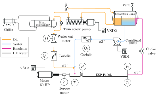
The ESP impellers have mixed flow geometry with an outer diameter of 108 and have $7$ blades. Pressure gauges and temperature transmitters were installed at the inlet and outlet of the ESP. They measure the suction and discharge pressure and temperature, respectively. The pressure transducers are capacitive and manufactured by Emerson Rosemount^™, series 2088. The temperature transducers are four-wire resistance temperature detectors type PT100 with 1/10 DIN accuracy. The pump shaft torque and rotational speed are measured using the sensor model T21WN manufactured by HBM^®. Each pump on the experimental setup is driven by an electric three-phase induction motor supplied by a Variable Speed Driver (VSD) on each motor.

The fluids used in the experiments are water and a blend of mineral oil. The oil viscosity was characterized by a rotational rheometer model HAAKE MARS III (see Section A.1 for the viscosity measurements in different temperatures). The water fraction inside the oil phase is measured by the water cut meter model Nemko 05 ATEX 112 manufactured by Roxar^®. The Coriolis meters used to measure the density and the mass flow rates of the oil and water flow lines are model F300S355 manufactured by Micro Motion^®.

As the system operates in a closed loop, it tends to heat up and change the viscosity. Thus, the heat exchanger controls the fluid’s temperature and the viscosity inside the flow line. The temperature is regulated by monitoring the ESP inlet temperature ($T_{1}$). This temperature measurement is also used for calculating the working fluid viscosity. The heat exchanger (HE) has an independent water flow line comprised of a chiller, a heater, and a water tank, allowing it to cool and heat the fluid. Also, as the oil viscosity strongly depends on the temperature, it is possible to conduct tests with different viscosities with the same oil by adjusting the fluid’s temperature.

The operational ranges and uncertainties of the instruments are presented in Table A.14. The specifications of the pumps, motors, variable speed drive, valve, tank, and heat control system are presented in Table A.13.

2.1.2 Experimental procedure

In this section, we detail the experimental procedure utilized to evaluate the dynamic behavior of the ESP system when varying the ESP shaft angular velocity while operating under a two-phase flow of oil and water. For simplicity, when referring to ESP angular velocity, it refers to the ESP shaft angular velocity. The procedure is divided into two stages; the first stage is the start-up stage, and the objective of this stage is to obtain a stable water cut. The second stage is the transient acquisition stage, in which we collect the experiment data.

1. Start-up:

   1. Begin by slowly starting the oil pump and water pump at a low speed (e.g., 62) to ensure system stability and prevent sudden pressure surges.

   2. Gradually increase the rotation speed of the ESP while monitoring the suction pressure. Maintain the ESP angular velocity below 105 and ensure the suction pressure remains above 100 to prevent cavitation in the ESP first stages.

   3. Check the measured water cut and adjust the water pump angular velocity if necessary. Repeat this step until the desired water cut is achieved.

   4. Stop the water pump.

2. Transient acquisition:

   1. Increase the ESP angular velocity to the desired initial value.

   2. Increase the oil pump angular velocity while closing the ESP downstream valve to maintain the suction pressure within the range of 100600. The upstream pressure of the ESP should not exceed 600 for a safe operation.

   3. Gradually increase the ESP angular velocity to reach the desired final value.

   4. Increase the oil pump angular velocity while closing the downstream valve to maintain the suction pressure within the range of 100600.

   5. Return the ESP angular velocity to the desired initial speed.

   6. Allow sufficient time for the suction, discharge pressure, and volumetric flow rate to stabilize. This stabilization period allows capturing only the dynamics of the ESP angular velocity change.

   7. Start data acquisition.

   8. Wait 5.

   9. Adjust the ESP angular velocity on the VSD to the final desired value.

   10. Allow another stabilization period for the suction, discharge pressure, and volumetric flow rate. This period allows the capture of the complete dynamic system response to the rotation change.

   11. End data acquisition.

   12. Return to the Stage 1:c

We considered the system stable when the coefficient of variation of the last 20 of measurements of the suction and discharge pressure and oil volumetric flow rate were smaller than 0.8. These criteria are the same as used and described by [41]. Additionally, for the temperature, we considered a tolerance of ±0.25 during the acquisition of the experimental time. The Supervisory Control and Data Acquisition (SCADA) system automatically monitors for the system stabilization and performs the steps Stage 2:f to Stage 2:k automatically.

2.1.3 Experimental investigation

Our experimental investigations focused on two different water-in-oil emulsion conditions. We varied parameters such as water fraction, temperature, and angular velocity step size. The specific values used in each experiment are presented in Table 1. By employing this approach, we were able to evaluate the system dynamics across different density and viscosity conditions while also assessing the influence of emulsion formation on the ESP.

Table 1: Test matrix for assessing the dynamics of the ESP system in oil/water two-phase flows. The table includes the experimental parameters varied in the study, such as the initial angular velocity ($\omega_{i}$), final angular velocity ($\omega_{f}$), water cut ($\Omega$), temperature, and twin-screw pump angular velocity ($\omega_{t}$).

Investigation (#)	$\omega_{i}$ ()	$\omega_{f}$ ()	$\Omega$ ()	Temperature ()	$\omega_{t}$ (RPM)
1	$272.27$	$314.16$	$14$	$33.5$	$1280$
2	$251.32$	$314.16$	$5$	$26$	$1160$

2.1.4 Data collection

We developed the SCADA system and implemented it using LabVIEW^™software. It gathers real-time data to monitor and control the ESP. We used a data acquisition system from National Instruments model cDAQ9188 to read and generate analog signals. The generated analog signals are sent to the pumps’ VSDs and valve actuators. We defined a sampling rate of 250 for the signal acquisition. The signals from different measuring instruments are collected simultaneously to ensure synchronized data acquisition.

An anti-aliasing filter was employed as a post-processing step on the acquired signals to remove high-frequency noise and ensure accurate signal acquisition. This low-pass filter is an 8${}^{\text{th}}$ order Butterworth filter with a cut-off frequency of 10. This frequency was chosen to comply with the Nyquist-Shannon sampling theorem for the maximum frequency specified by the pressure transmitter manufacturer. Then, the signal was downsampled to the same frequency.

2.2 Electrical submersible pump system dynamic model

In this section, we describe the dynamic behavior of the ESP system by using a set of Ordinary Differential Equations (ODEs), derived from a bond graph representation of the system (presented in Figure B.1 in Appendix B). The model is based on the works of [42, 43], which provide bond graph models for centrifugal pumps and pipelines, respectively. In this study, we focused only on the mechanical and hydraulic domains of the system for simplicity. Therefore, the electrical motor was not considered in this model. Instead, we treated the shaft torque as an input to the system, decoupling the mechanical and electrical domains.

The ESP system is described by the state variable,

$$\bm{X}=\{Q_{p},\omega,Q_{1},Q_{2},P_{1},P_{2}\},$$ (1)

where $Q_{p}$ is the pump volumetric flow rate, $\omega$ is the shaft angular velocity, $Q_{1}$ and $Q_{2}$ are the volumetric flow rate in the upstream and downstream pipeline respectively, $P_{1}$ and $P_{2}$ are the intake and discharge pressure respectively. The governing equations describing the dynamics of the system depend on the input vector $\gamma(t)$. These are of the form

$$\bm{\dot{X}}=F(\bm{X},\gamma(t)).$$ (2)

The ESP system is governed by the following set of ODEs:

$$\frac{dQ_{p}}{dt}=\frac{(P_{1}-P_{2}+k_{3}\,\mu\,Q_{p})\,A_{p}}{\rho\,L_{p}}+\frac{A_{p}\,(k_{1p}\,\omega\,Q_{p}+k_{2p}\,\omega^{2}+k_{4p}\,{Q_{p}}^{2})}{L_{p}},$$ (3a)

$$\frac{d\omega}{dt}=\frac{\gamma(t)-k_{1s}\,\rho\,{Q_{p}}^{2}-k_{2s}\,\rho\,\omega\,Q_{p}-k_{3s}\,\mu\,\omega-k_{4s}\,\omega-k_{5s}\,\omega^{2}}{I_{s}},$$ (3b)

$$\frac{dQ_{1}}{dt}=\frac{(k_{bd}\omega_{t}-Q_{1})\,k_{bl}\,\mu+P_{in}-P_{1}-f_{f}(Q_{1},\mu,L_{u},d_{u})\,{Q_{1}}^{2}\,A_{u}}{\rho\,L_{u}}-\frac{k_{u}\,{Q_{1}}^{2}}{2\,L_{u}\,A_{u}},$$ (3c)

$$\frac{dQ_{2}}{dt}=\frac{(P_{2}-P_{out}-f_{f}(Q_{2},\mu,L_{d},d_{d})\,{Q_{2}}^{2})\,A_{d}}{\rho\,L_{d}}-\frac{k_{d}\,{Q_{2}}^{2}}{2\,L_{d}\,A_{d}}-\frac{{Q_{2}}^{2}\,A_{d}}{L_{d}\,C_{v}(a)^{2}\,\rho_{0}},$$ (3d)

$$\frac{dP_{1}}{dt}=\frac{(Q_{1}-Q_{p})\,B}{A_{u}\,L_{u}},$$ (3e)

$$\frac{dP_{2}}{dt}=\frac{(Q_{p}-Q_{2})\,B}{A_{d}\,L_{d}},$$ (3f)

where the parameters are described in detail in Appendix B, the function $C_{v}(a)$ represents the valve coefficient as a function of the valve aperture ($a$), and $\rho_{0}$ is the water density at 15. For simplicity, as we are not varying the valve aperture, we considered a single equivalent resistance coefficient obtained experimentally.

Considering the high viscosity of the emulsion, we assumed a laminar flow in the emulsion and oil flow lines. Therefore, the friction function $f_{f}(Q,\mu,L,d)$ is derived using the Darcy-Weisbach equation and the friction factor for laminar flow, resulting in the following equation:

$$f_{f}(Q,\mu,L,d)=\frac{128\,L\,\mu}{\pi\,Q\,d^{4}}.$$ (4)

The ESP system model takes a single input variable, $\gamma(t)$, representing the torque applied to the ESP shaft. In the experimental setup, the intake pressure of the twin-screw pump $P_{in}$ and the pressure at the end of the pipeline $P_{out}$ refers to the same separation tank that is open to the atmosphere. Therefore, for the sake of simplicity, these pressures are assumed to be constant and are set to 0.

It is important to mention that in both experimental and real-world conditions, various factors, such as turbulence and shear generated by the ESP, valve, and other devices installed in the flow line, contribute to emulsion formation, leading to changes in emulsion viscosity. Thus, the viscosity of the emulsion varies as the fluids traverse the system due to these effects. Additionally, the emulsion formation is influenced by the emulsion stability, chemical properties of the fluid, and the presence or addition of emulsifiers and surfactants. Moreover, in practical scenarios, temperature gradients along the pipeline significantly impact viscosity. In such cases, the assumption of a single viscosity is no longer valid, and appropriate assumptions must be made to account for these complexities.

In our specific case, the ESP operates within a closed-loop system. Consequently, the same emulsion continuously flows through the ESP and valves while the fluid temperature is controlled through a heat exchanger. Given the tank volume, the operating volumetric flow rate, temperature control measures, and the transient experiment duration, we assumed that viscosity remains approximately constant.

Although the [44] model is widely used in the oil industry for emulsion effective viscosity, numerous alternative models for emulsion viscosity have been proposed (e.g., [45], [46] and [47]). Recently, [12] introduced a model specifically for effective emulsion viscosity inside ESPs. However, this model is exclusively applicable to ESPs and does not hold for pipelines. Thus, in this study, we employed the [44] model to determine the emulsion viscosity for the entire system, it is expressed as:

$$\mu=\mu_{c}\left(\frac{1}{1-\Omega}\right)^{2.5}\quad\quad 0<\Omega<1,$$ (5)

where $\Omega$ represents the water cut and $\mu_{c}$ is the viscosity of the continuous phase

2.3 Physics-informed neural networks

The physics-informed neural network (PINN) comprises of a neural network (NN) to approximate the solution of a given differential equation and a second part that is considered to encode the corresponding differential equation in the optimization of the network parameters. The differential equation is encoded in the loss function along with data loss with the help of automatic differentiation [31]. In this study, we consider a fully connected feed-forward deep neural network (DNN) to approximate the state variables (i.e. $Q_{p}$, $\omega$, $Q_{1}$, $Q_{2}$, $P_{1}$, $P_{2}$). The DNN architecture comprises one input layer, $h$ hidden layers, and one linear output layer and can be represented as follows:

$$\bm{y}_{0} =t\hskip 180.67517pt$$ Input (6a)

$$\bm{y}_{i} =\sigma\left(\bm{W}_{i}\bm{y}_{i-1}+\bm{b}_{i}\right)\hskip 28.45274pti\;\forall\;1\leq i\leq h-1\hskip 28.45274pt$$ Hidden layers (6b)

$$\bm{\hat{y}}=\bm{y}_{h} =\bm{W}_{h}\bm{y}_{h-1}+\bm{b}_{h-1}$$ Output layer (6c)

where $\bm{W}\in\mathbb{R}^{m\times n}$ and $\bm{b}\in\mathbb{R}^{m}$ are the weights and biases of the neural network. The $n$ and $m$ are the sizes of the previous and current layers, respectively. The function $\sigma(.)$ is the activation function, which in this study we consider as a $\text{tanh}(.)$ function. For the remainder of this work, the weights and biases are referred to collectively as parameters of the neural network $\bm{\theta}=\{\bm{W},\bm{b}\}$.

The schematic diagram of the PINN considered in this study is presented in Figure 2. In this work, a single DNN approximates the set state variables of the ODEs presented in Section 2.2. This approach has demonstrated satisfactory results while maintaining a lower computational cost than training separate DNNs for each state variable.

Fig. 2: Schematic representation of the Physics-informed neural network for the ESP system: The deep neural network, shown in the red dashed-dotted rectangle on the left, is considered to approximate the solution of the ODEs system described in Section 2.2 (Equations 3a to 3f). The input to the neural network is time, denoted by $t$, and the output is the ESP system states, highlighted in the green dotted rectangle of the figure. Each differential equation of the ESP system has residues at certain collocation points that must be minimized. We indicate them in the black dotted region on the right. The time derivative of each state (DNN output) is computed using automatic differentiation. The total loss, denoted as $\mathcal{L}(\bm{\theta})$, includes data loss, physics (ODE) loss, and initial condition loss. The data loss ($\mathcal{L}^{data}(\hat{y}-y))$ is the loss between the DNN output and measured data, the physics (ODE) loss is the loss of the residue of the equations at the collocation points, and the initial condition loss is a loss between the initial condition and the DNN output at $t=0$. $\bm{\lambda}_{d}$, $\bm{\lambda}_{r}$, and $\bm{\lambda}_{ic}$ are the weights to the data loss, physics loss, and initial condition loss, respectively, while calculating the total loss. These may be fixed or adaptive. $\bm{\Lambda}$ are the unknown parameters in the ODE system. The activation function of the DNN is represented by $\sigma$.

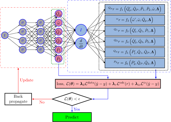
The loss consists of three different losses, i.e., the physics loss ($\mathcal{L}^{ode}(\bm{\theta},\bm{\Lambda},\bm{\lambda}_{r}$)), the data loss ($\mathcal{L}^{data}(\bm{\theta},\bm{\lambda}_{d})$) and the initial condition loss ($\mathcal{L}^{ic}(\bm{\theta},\bm{\lambda}_{ic}$)). The total loss is given as,

$$\mathcal{L}(\bm{\theta},\bm{\Lambda},\bm{\lambda}_{d},\bm{\lambda}_{r},\bm{\lambda}_{ic})=\mathcal{L}^{ode}(\bm{\theta},\bm{\Lambda},\bm{\lambda}_{r})+\mathcal{L}^{data}(\bm{\theta},\bm{\lambda}_{d})+\mathcal{L}^{ic}(\bm{\theta},\bm{\lambda}_{ic}).$$ (7)

The physics loss is given by the weighted sum (self-adaptive weights) of physics loss due to individual equation,

$$\mathcal{L}^{ode}(\bm{\theta},\bm{\Lambda},\bm{\lambda}_{r}) =\sum_{s\in\Phi}m(\lambda_{r}^{s})\mathcal{L}^{ode}_{s},\qquad\Phi=\{Q_{p},\;\omega,\;Q_{1},\;Q_{2},\;P_{1},\;P_{2}\},$$ (8a)

$$=\sum_{s\in\Phi}m(\lambda_{r}^{s})\left[\frac{1}{{{}^{s}}N^{ode}}\sum_{i=1}^{{{}^{s}}N^{ode}}{{{}^{s}}r_{i}}^{2}\right],$$ (8b)

$$=\sum_{s\in\Phi}m(\lambda_{r}^{s})\left[\frac{1}{{{}^{s}}N^{ode}}\sum_{i=1}^{{{}^{s}}N^{ode}}\left(\frac{d\hat{y_{s}}}{dt}\middle|_{t_{i}}-f_{s}\left(\hat{y}(t_{i};\bm{\theta}),\gamma(t_{i});\bm{\Lambda}\right)\right)^{2}\right],$$ (8c)

where $\mathcal{L}^{ode}_{s}$, $s\in\Phi$, $\Phi=\{Q_{p},\;\omega,\;Q_{1},\;Q_{2},\;P_{1},\;P_{2}\}$ are the physic-informed loss for the differential equation describing the dynamics of the state variables (Equations 3a to 3f). ${}^{s}N^{ode}$ is the number of residual points for each of the equations, $\lambda_{r}^{s}$ are the self-adaptive weights associated with each physics loss, and $m(.)$ is a mask function which is considered as softplus function in the present study. ${}^{s}r_{n}$ are the residual of the equation. We discuss the calculation of the residual in Appendix C. In the present study, the residual points for all the equations are considered the same. Thus, all ${}^{s}N^{ode}$ has the same points.

Similarly, the data loss is given by the weighted sum (self-adaptive weights) of data loss due to $P_{1}$ and $P_{2}$.

$$\mathcal{L}^{data}(\bm{\theta},\bm{\lambda}_{d}) =\sum_{s\in\phi}m(\lambda_{d})\mathcal{L}^{data}_{s},\qquad\phi=\{P_{1},\;P_{2}\}$$ (9a)

$$=\sum_{s\in\phi}m(\lambda_{d})\left[\frac{1}{{}^{s}N^{data}}\sum_{i=1}^{{}^{s}N^{data}}\left[y_{s}(t_{i})-\hat{y}_{s}(t_{i};\bm{\theta})\right]^{2}\right],$$ (9b)

where ${}^{s}N^{data}$ is the number of points at which the measured data are available for each of the known quantities, $y_{s}(t_{i})$ is the known value of the $s$ quantity at time $t_{i}$ and the corresponding approximated value from the neural network is $\hat{y}_{s}(t_{i};\bm{\theta})$. Similar to physics loss, $\lambda_{d}^{s}$ is the self-adaptive weight associated with each data loss, and $m(.)$ is a mask function taken as the softplus function in the present study.

The initial condition loss

$$\mathcal{L}^{ic}(\bm{\theta},\bm{\lambda}_{ic}) =\sum_{s\in\Phi}m(\lambda_{ic}^{s})\mathcal{L}^{ic}_{s},\qquad\Phi=\{Q_{p},\;\omega,\;Q_{1},\;Q_{2},\;P_{1},\;P_{2}\}$$ (10a)

$$=\sum_{s\in\Phi}m(\lambda_{ic}^{s})\left[\left(y_{s}(t_{0})-\hat{y}_{c}(t_{0};\bm{\theta})\right)^{2}\right],$$ (10b)

where $y_{s}(t_{0})$ is the known value of the $s$ quantity at time zero, and the corresponding approximated value from the neural network is $\hat{y}_{s}(t_{0};\bm{\theta})$. $m(.)$ is a mask function taken as the softplus function in the present study.

The neural network architecture considered in the present study is $[1,20,20,20,6]$, where the input layer consists of one neuron that takes time $t$ as input and is scaled between $[-1,1]$. In the output layer, we have six neurons that approximate the six state variables discussed in Section 2.2 (Equation 3a to Equation 3f). The neural network outputs pass through a transformation given by:

$$f(x)=\frac{(x+1)(x_{\text{max}}-x_{\text{min}})}{2}+x_{\text{min}}$$ (11)

where $f(x)$ represents the state variable in the physical domain, and $x$ is the output from the neural network. For known states (i.e., $P_{1}$ and $P_{2}$), $x_{\text{min}}$ and $x_{\text{max}}$ are the minimum and maximum measured values, respectively. However, for the unknown states, the $x_{\text{min}}$ and $x_{\text{max}}$ are estimated by solving a system of equations at two specific time points $t_{1}$ and $t_{2}$. The system of equations, derived from simplifications of Equations 3a and 3b, is given by:

$$\begin{cases}k_{1p}\,\rho\,\omega(t_{i})\,Q_{p}(t_{i})+k_{2p}\,\rho\,\omega(t_{i})^{2}+k_{4p}\,\rho Q_{p}(t_{i})^{2}-(P_{2}(t_{i})-P_{1}(t_{i}))=0,\\ k_{1s}\,\rho\,Q_{p}(t_{i})^{2}-k_{2s}\,\rho\,\omega(t_{i})\,Q_{p}(t_{i})+\gamma(t_{i})=0,\quad\quad t_{i}\in\{t_{1},t_{2}\}\end{cases}$$ (12)

where $k_{1p}$, $k_{2p}$, $k_{4p}$, $k_{1s}$, and $k_{2s}$ are the ESP system parameters, $\rho$ represents the fluid density, and $t_{i}$ denotes the time instant for the state variables ($\omega$, $Q_{p}$, $P_{1}$, $P_{2}$) and system input ($\gamma$). Furthermore, the time points $t_{1}$ and $t_{2}$ are determined based on the pressure difference between $P_{2}(t)$ and $P_{1}(t)$ as follows:

$$t_{1}=\arg\min_{t}\left(P_{2}(t)-P_{1}(t)\right),\quad t_{2}=\arg\max_{t}\left(P_{2}(t)-P_{1}(t)\right).$$ (13)

Solving the system of equations at the time point $t_{1}$ provides the estimation for $x_{\text{min}}$, and at the time point $t_{2}$ for $x_{\text{max}}$. We would also like to mention that in order to solve the above Equation 12, we need to know the parameters ($k_{1p}$, $k_{2p}$, $k_{4p}$, $k_{1s}$ and $k_{2s}$) of the equation, which are unknown in this case. Thus, we assumed some initial value in the parameters. In this study, while solving the Equation 12, we considered $\rho=\qty{931.51}{\per\cubic}$, which represents a water cut of 50, as an initial guess, and for the remaining pump parameters we considered a value of $+15\%$ of the true value for all parameters. Additionally, we considered the same values obtained for $Q_{p}$ for the $Q_{1}$ and $Q_{2}$ states (pipeline flow rates).

It is also worth noting that the state variables are at different scale (magnitude). To address this, we employ the transformation, described by Equation 11, to make the neural network’s output of similar order for different state variables. This transformation can be of different forms, depending on the specific requirements of the problem. In the present study, the bounds $x_{\text{min}}$ and $x_{\text{max}}$ vary across the different experimental investigations as they depend on $P_{2}(t)$ and $P_{1}(t)$.

The trainable parameters ($\bm{\theta}$, $\bm{\Lambda}$, $\bm{\lambda}_{d}$, $\bm{\lambda}_{r}$ and $\bm{\lambda}_{ic}$) are optimized using the Adam optimizer. The automatic differentiation for the derivatives of the outputs with respect to input is evaluated using the Python library JAX, while the Adam optimization is carried out using the Optax library. As discussed earlier, we have considered self-adaptive weight [37]. Thus, we considered different optimizers (three) for the neural network parameters (weights and biases), unknown parameters, and self-adaptive weights. We discuss the number of training epochs and learning rate scheduler in detail in Appendix D for each numerical example. Further, the unknown parameters transformations will be discussed in Section 4.

2.4 Data generation

In this study, we considered laboratory data collected from the experimental setup described in Section 2.1. Before considering the proposed PINN model for experimental data, we test out the model with simulated with and without noise. The simulated data are generated by solving the ODEs system presented in Section 2.2. This section will present the steps for generating the simulated data. We define the parameters and input used in the simulations. We try to generate the simulated data as close as to the experimental data making the parameters and the input of the system near equal to the experimental setup, and are discussed hereafter.

For the simulated cases, in this study, we employed the Julia package DifferentialEquations.jl [48] to numerically solve the ESP system set of ODEs presented in Section 2.2. The simulated data were generated with $\Delta t=\qty{0.0001}{}$.

The model input is the torque ($\gamma(t)$), which we directly measured during each experimental investigation. After post-processing the torque signal, as described in Section 2.1.4, we observed that the torque signal still contained relatively high-frequency components, which would be unrealistic as an input for the ESP system. Therefore, we applied a Butterworth low-pass filter with a cut-off frequency of 2 to the torque signal to obtain a more representative input signal.

For fluid viscosity, we assumed a single value for the entire system. We calculated the average water cut and temperature observed during the corresponding experimental investigation and estimated the emulsion viscosity using the [44] model. As for fluid density, we directly measured it using a Coriolis meter. Then, we calculated the average density obtained from the measurements conducted during each experimental investigation.

In the tuning step of a dynamic model, the parameters are adjusted to fit real-world observations. However, despite the tuning step, we expect discrepancies between the model predictions and measured data. They arise due to uncertainties in the data and the model’s representation of the actual system, which may not fully capture the system complexities. Additionally, in inverse problems, minor variations or errors in the fixed parameter can significantly affect the desired parameter estimation.

Therefore, to accurately evaluate the capability of PINNs in handling measurement uncertainties while excluding potential influences of missing physics or the tuning steps, we incorporated Gaussian noise into the simulated signals $P_{1}$ and $P_{2}$. The noise values used in these signals were determined based on the manufacturer’s specifications for the pressure transmitters’ uncertainties, as detailed in Table A.14.

2.5 Structural identifiability analysis

In the Section 2.2, we introduced a set of ODE that describes the ESP system dynamics that has $26$ parameters and $6$ states variables. Before trying to estimate the unknown parameters of the system using the PINN, it is important to assess whether or not the parameters can be uniquely determined from a given set of data.

Consider a dynamical system in the following format

$$\dot{\bm{x}}(t)=\bm{f}(\bm{x}(t),\bm{u}(t),\bm{\Theta}),$$ (14)

$$\bm{y}(t)=\bm{h}(\bm{x}(t),\bm{u}(t),\bm{\Theta}),$$ (15)

where $\bm{x}(t)$ is an $m$-dimensional state vector, $\bm{u}(t)$ is an $n$-dimensional input signal, $\bm{y}(t)$ is an $r$-dimensional output signal or the measurable output, and $\bm{\Theta}$ is $k$-dimensional vector of parameters. A parameter set $\bm{\Theta}$ is said to be structurally globally identifiable if the following property holds:

$$\bm{h}(\bm{x}(t),\bm{u}(t),\bm{\Theta})=\bm{h}(\bm{x}(t),\bm{u}(t),\bm{\beta})\implies\bm{\Theta}=\bm{\beta},$$ (16)

where $\bm{\beta}$ is a $k$-dimensional vector of parameters. Furthermore, if the property in Equation 16 holds within a neighborhood of $\bm{\Theta}$, it is referred to as structurally locally identifiable.

Thus, the identifiability property serves as a prerequisite for practical parameter estimation. Additionally, as stated by [49], if a parameter is locally identifiable, it implies that the search range for that parameter should be limited before attempting its estimation. On the other hand, for globally identifiable parameters, there is no need to define a search range.

3 Results and discussions for identifiability analysis

3.1 Local identifiability

We utilized the method of differential elimination for dynamical models via projections proposed by [23] to evaluate the structural identifiability of the ESP system model. It is important to note that our analysis focused specifically on assessing local identifiability due to out-of-memory issues when attempting to test for structural global identifiability. Additionally, our investigation considered the suction and discharge pressure ($P_{1}$ and $P_{2}$) as available measurements, as they are typically measured in ESP deployments within oil fields.

From Tables B.1 and B.2, we observe that the ESP system model initially contains a total of $26$ parameters. However, it is worth noting that $8$ of these parameters are geometrical parameters, such as pipe diameter, cross-sectional area, and pipeline length. They can be readily obtained, and they were fixed for both the upstream and downstream pipelines. Furthermore, $3$ parameters refer to the twin-screw pump, which serves as a pressure booster for the flow line. In actual oil field extraction, the pressure is a characteristic of the well. Thus, we reduce the number of unknown parameters to $15$. Subsequently, we assessed the local identifiability of the ESP system model based on these $15$ parameters. The corresponding results are displayed in the first row of Table 2.

Table 2: Local structural identifiability results of the ESP system model, considering that the intake pressure ($\bm{P_{1}}$) and discharge pressure ($\bm{P_{2}}$) are known. The symbols $\times$indicate locally unidentifiable parameters, ✓indicate locally identifiable parameters, and $-$  represent fixed parameters.

$k_{1p}$	$k_{2p}$	$k_{3p}$	$k_{4p}$	$k_{1s}$	$k_{2s}$	$k_{3s}$	$k_{4s}$	$k_{5s}$	$I_{s}$	$\rho$	$\mu$	$B$	$k_{u}$	$k_{d}$
$\times$	$\times$	✓	✓	$\times$	$\times$	$\times$	$\times$	$\times$	$\times$	✓	✓	✓	✓	✓
✓	✓	✓	✓	✓	✓	$\times$	$\times$	✓	$-$	✓	✓	✓	✓	✓
✓	✓	✓	✓	✓	✓	$-$	$-$	✓	$-$	✓	✓	✓	✓	✓

The ESP system model with $15$ unknown parameters is found to be structurally locally unidentifiable, and it is impossible to estimate all of the parameters simultaneously. As discussed by [49], there are several approaches to address the identifiability issue, such as fixing specific parameters or introducing additional measured variables. For simplicity, when we refer to fixing a parameter, we consider that the parameter is known. In this study, we opted to work with the available measurements from the actual field and consider only the suction and discharge pressures ($P_{1}$ and $P_{2}$). Therefore, we decided to fix the shaft inertia ($I_{s}$). Despite this adjustment, the model remains structurally locally unidentifiable, with only $k_{3s}$ and $k_{4s}$ being locally unidentifiable. The corresponding results are shown in the second row of Table 2.

Finally, we solved the issue of the model being locally unidentifiable by fixing both $k_{3s}$ and $k_{4s}$. The results are shown in the third row of Table 2. We found that fixing only one of them did not solve the problem. In summary, the ESP system model can only be structurally locally identifiable with the suction and discharge pressure measurements if the shaft inertia ($I_{s}$), viscous damping coefficient ($k_{4s}$), and disk friction coefficient ($k_{3s}$) are known.

3.2 Practical identifiability

In section Section 3.1, we discussed the circumstances under which the ESP system is structurally locally identifiable. However, it is worth noting that this analysis was conducted assuming that the measured variables have no noise and that the model is error-free. Hence, we must also assess if we can estimate parameters accurately based on the available data’s quantity and quality. This analysis is known as practical or posterior identifiability analysis, and it is possible that a structurally identifiable system may not be practically identifiable.

The practical identifiability can be assessed using either Monte Carlo simulations or sensitivity analysis. The Monte Carlo approach rigorously determines the practical identifiability of the model but comes with a high computational cost due to the requirement of multiple model fits. On the other hand, sensitivity analysis offers a faster computation method and provides information about the correlation structure among the parameters. This correlation structure can guide the fixing of parameters when practical identifiability is not achieved [19, 50].

In this study, we considered only the sensitivity approach to practical identifiability. Then, we used the Fisher information matrix (FIM) to compute the correlation matrix of all parameters to determine their practical identifiability. We estimate the sensitivities of the ESP system model with respect to the parameters with the Julia package DiffEqSensitivity.jl. For the sensitivity analysis, we considered the simulated case, and similarly to [49], we considered a noise level of the measurements of 1.

Then, to obtain the correlation matrix, we first estimate the covariance matrix ($\bm{C}$) which can be approximately obtained from the FIM by

$$\bm{C}=FIM^{-1}.$$ (17)

We then estimate the correlation matrix from ($\bm{C}$) with

$$\begin{cases}r_{ij}=\frac{\bm{C}_{ij}}{\sqrt{\bm{C}_{ii}\,\bm{C}_{jj}}},&\text{if }i\neq j,\\ r_{ij}=1,&\text{if }i=j.\\ \end{cases}$$ (18)

When $|r_{ij}|$ is close to $1$, the parameters $i$ and $j$ are strongly correlated and cannot be individually estimated. Therefore, the parameters are practically unidentifiable [19, 50]. The absolute of the correlation matrix of the parameters structurally locally identifiable of the ESP system is shown in Figure 3(a). For the practical identifiability analysis, we considered the simulated case for the first investigation of the test matrix, Table 1.

(a) Twelve unknown parameters.

(b) Eight unknown parameters.

Fig. 3: Absolute values of the estimated correlation matrices for ESP system model parameters. The matrices are derived based on the FIM. The matrix indicates whether parameters are identifiable or not. Parameters with absolute correlation values near 1 are practically unidentifiable. The Figure 3(a) represents twelve structurally locally identifiable parameters, while the Figure 3(b) focuses on eight parameters, particularly keeping fluid properties and pipeline resistances unknown.

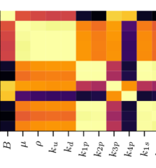
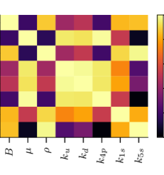
The correlation analysis shown in Figure 3(a) clearly demonstrates a significant correlation among multiple parameters. Notably, the fluid density ($\rho$) and the pipeline resistances ($k_{u}$ and $k_{d}$) exhibit a strong correlation. Consequently, although the initial analysis indicated structural local identifiability of these parameters, they are not practically identifiable within the context of the conducted investigation.

As many parameters are strongly correlated, we need to fix some parameters to make the system practically identifiable. We set that the main variables of interest are the fluid parameters and the pipeline resistances since the fluid parameters ($B$, $\mu$, and $\rho$) change within the water cut, which changes with the well’s life, and the pipeline resistance ($k_{u}$ and $k_{d}$) changes with the actuation of valves and wax deposition for instance. Thus, we preferably fixed the pump and shaft parameters. We started by fixing the parameter $k_{1p}$, then the $k_{3s}$, $k_{2p}$ and $k_{3p}$ successively. The resultant parameter correlation matrix is presented in Figure 3(b).

It is noticeable from Figure 3(b) that after fixing some parameters, they are less correlated. However, some parameters are still correlated, such as the viscosity ($\mu$) and the pump equivalent resistance ($k_{4p}$). However, this correlation is not as strong as the correlation between density ($\rho$) and pipeline resistance ($k_{u}$) observed in Figure 3(a). In Figure 3(b), the correlation coefficient between $\mu$ and $k_{4p}$ is $0.988\,021$, while in Figure 3(a), the correlation coefficient between $\rho$ and $k_{u}$ is $0.999\,359$.

4 Results and discussions for inverse problem using PINN

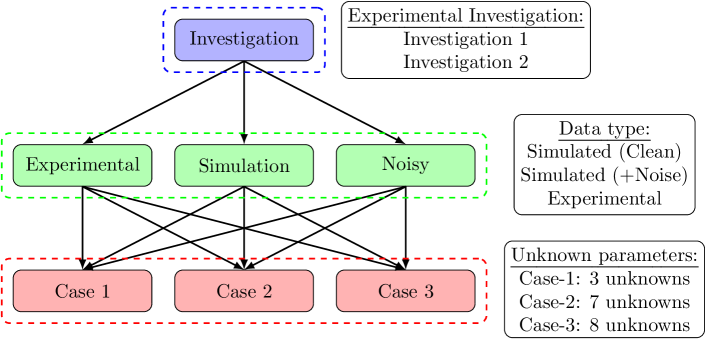
From the structural identifiability analysis presented in Section 3, we have defined three cases to evaluate the PINN for parameter and state estimation in the ESP system. Consistent with Section 3, we considered only the suction and discharge pressures as the measured variables. The three cases are as follows:

1. Flow parameters: In this case, we assumed as known all parameters of the ESP system model except for the flow properties, namely, density ($\rho$), viscosity ($\mu$), and the bulk modulus ($B$).

2. Flow, pipeline, and impeller parameters: Based on the local identifiability analysis results presented in the first row of Table 2, we assumed as known the parameters marked as locally unidentifiable and estimate the remaining identifiable ones. The unknown parameters considered are the flow properties ($B$, $\mu$, $\rho$), the upstream pipeline equivalent resistances ($k_{u}$ and $k_{d}$) and the pump parameters $k_{3p}$ and $k_{4p}$.

3. Flow, pipeline, impeller, and shaft parameters: Considering the findings from the practical identifiability analysis outlined in Section 3.2, we estimate the parameters depicted in Figure 3(b) while assuming as known the remaining parameters. The unknown parameters are fluid properties ($B$, $\mu$, $\rho$), the upstream pipeline equivalent resistances ($k_{u}$ and $k_{d}$), the pump parameter $k_{4p}$, and the shaft parameters $k_{1s}$ and $k_{5s}$.

For each case, we will evaluate the performance and effectiveness of PINN in estimating the unknown parameters and non-measured system states in three distinct data scenarios:

1. Simulated data: This scenario represents an ideal condition without any disturbances or modeling errors, allowing us to assess the baseline performance of the proposed method.

2. Simulated data with Gaussian noise: In this scenario, we introduce Gaussian noise to the simulated data to evaluate the sensitivity of the proposed method to noisy data.

3. Experimental data: This scenario is closer to actual oil field conditions, incorporating noisy measurements, modeling errors, and missing information about certain parameters.

Furthermore, for each study, we trained the PINN $30$ times to evaluate the impact of the neural network weights initialization. The results are presented and discussed in each case for the two experimental conditions defined in Table 1. Figure 4 presents a schematic representation of the cases and scenarios evaluated.

Fig. 4: Cases and scenarios evaluated. As presented in Section 2.1.3, two experimental investigations (blue) are performed, considering different water cuts and initial angular velocities. Each experimental investigation is analyzed under three different data sources (scenarios): simulation data, simulation data with added Gaussian noise, and experimental data collected from the instruments (green). For each scenario, three sets of unknown parameters, denoted as cases, are evaluated (red). Thus, we have $9$ different results for each experimental investigation.

During the training of the PINN, we observed that the significant difference in magnitude between the states, with pressure in the order of $10^{5}$ and flow rates in the order of $10^{-2}$, affected the training and tuning process despite the scaling in the physics loss and the usage of self-adaptive weights on the loss function. Therefore, we converted the units of the states from SI units to for the volumetric flow rates and to MWC (meters of water column) for the pressure. After obtaining the results, we converted them back into SI units.

Furthermore, the transformation of the unknown parameters contributes to the convergence and accuracy of the PINN by restricting the search space to the local neighborhood of the parameter. We first tried to keep the linear scaling for all parameters and cases during the development. However, in Case 3, we could not achieve satisfactory results without restricting the parameter search space using bounded transformations such as $\tanh$. Also, we took advantage of that in our experiments. It is not possible to have a density higher than the water. Then, we set an upper bound for it. It helped to improve the results in all cases. The transformation scheme for each parameter is shown in Table 3, and the scaling values are presented in Table 4.

Table 3: Transformations of the unknown parameters for each case evaluated. The transformations applied to the unknown parameters are detailed. The softplus function $S_{p}(\cdot)$ and the $S_{m}(\cdot)$, defined as $S_{m}(x)=x-\text{softplus}(x)+1$, are utilized along with a scaling constant $\Lambda$. The $L(\cdot)$ is a linear transformation given by $L(x)=x\Lambda$, which considers only a scaling constant $\Lambda$. For Case 3, the transformation for an unknown parameter is expressed as $\Lambda_{\text{sc}}(x)=\Lambda_{\text{true}}\left(\tanh(x)\alpha+1\right)$, where $x$ represents the PINN-estimated value of the unknown parameter, $\Lambda_{\text{true}}$ is the parameter true value, and $\alpha$ denotes the span percentage around the true value. For most parameters, we set the span to $\pm 50\%$ ($\alpha=0.5$), except for the $B$ parameter, which spans $\pm 15\%$ ($\alpha=0.15$).

Case	$B$	$\mu$	$\rho$	$k_{u}$	$k_{d}$	$k_{3p}$	$k_{4p}$	$k_{1s}$	$k_{5s}$
Case 1	$(S_{p}(x)+0.9)\Lambda$	$L(x)$	$S_{m}(x)\Lambda$
Case 2	$(S_{p}(x)+0.9)\Lambda$	$L(x)$	$S_{m}(x)\Lambda$	$L(x)$	$L(x)$	$L(x)$	$L(x)$
Case 3	$\Lambda_{\text{sc}}(x)$	$\Lambda_{\text{sc}}(x)$	$S_{m}(x)\Lambda$	$\Lambda_{\text{sc}}(x)$	$\Lambda_{\text{sc}}(x)$		$\Lambda_{\text{sc}}(x)$	$\Lambda_{\text{sc}}(x)$	$\Lambda_{\text{sc}}(x)$

Table 4: Scaling constants for the unknown parameters. The table presents the scaling constants used in linear parameter transformations and the scaling parameter for the liquid bulk modulus ($B$) and density ($\rho$) transformations.

Case	$B$	$\mu$	$\rho$	$k_{u}$	$k_{d}$	$k_{3p}$	$k_{4p}$
Case 1	$1\text{\times}{10}^{9}$	$1$	$1000$
Case 2	$1\text{\times}{10}^{9}$	$1$	$1000$	$3.0\text{\times}{10}^{2}$	$1.0\text{\times}{10}^{1}$	$-1.0\text{\times}{10}^{7}$	$-1.0\text{\times}{10}^{2}$
Case 3			$1000$

4.1 State estimation results

We begin by assessing the state estimation capabilities of the PINN when applied to the ESP system model. The PINN will estimate the remaining unknown system states using the suction and discharge pressure signals as known variables ($P_{1}$ and $P_{2}$). In the simulated cases, the unknown states include the pipeline and ESP volumetric flow rates ($Q_{1}$, $Q_{2}$, $Q_{p}$) and the ESP angular velocity ($\omega$). However, in the experimental case, measurements of the downstream pipeline and ESP volumetric flow rates ($Q_{2}$ and $Q_{p}$) are unavailable, and therefore, they were excluded from the accuracy analysis. We would also like to mention that these results are from inverse problems with unknown parameters discussed above, not forward problems. First, we present the state estimation results for all the cases considered. Then, we discuss the prediction of the unknown parameters for all the cases in Section 4.2.

It is worth mentioning that in PINN, it is common practice to use second-order optimization algorithms, such as L-BFGS, after training with the first-order algorithm. This additional step usually aims to fine-tune the PINN’s performance. However, we observed that using L-BFGS after Adam adversely affected the parameter estimation in the noisy and experimental case. Therefore, we decided to rely solely on the first-order optimization algorithm, as our focus is on unknown parameter estimation in more realistic scenarios. It is important to note that the simulated cases serve as a baseline performance for assessing the PINN’s performance, and we expect that performance will be comparatively reduced under the more challenging conditions posed by experimental data and noise.

4.1.1 State estimation results for simulated data

As a baseline performance assessment, we begin with the simulated scenario. The predicted states from the neural network are shown in Figure 5, while the Mean Absolute Percentage Error (MAPE) corresponding to the prediction of different states is shown in Table 5. The MAPE is defined as

$$\text{MAPE}=\frac{1}{N^{mape}}\sum_{i=1}^{N^{mape}}\left|\frac{y_{s}(t_{i})-\bar{y}_{s}(t_{i};\bm{\theta})}{y_{s}(t_{i})}\right|,$$ (19)

where $N^{mape}$ is the total number of temporal data points. We considered the same sample rate as the experimental data described in Section 2.1.4, 10 ($\Delta t=0.1$ sec). The variable $y_{s}(t_{i})$ represents the true value of the state $s$ at time $t_{i}$, and $\bar{y}_{s}(t_{i};\bm{\theta})$ denotes the mean of the predicted value of the state $s$ from the PINN across 30 different realization of the results. These results are evaluated with different initialization of the parameters of the network and unknown parameters. For the sake of brevity, we restrict our discussion to the state prediction results and the MAPE table for the first experimental investigation. Further results from the second investigation are presented in Appendix E. We have shown the mean value of the predicted parameters and standard deviation for all the cases in Tables 11 and 12.

Table 5: MAPE for the simulated scenario. The table presents the results for the simulation data considering three different cases of unknown parameters. The MAPE values represent the error of the simulation results for the states: $P_{1}$, $P_{2}$, $Q_{1}$, $Q_{2}$, $Q_{p}$, and $\omega$. As the number of unknown parameters increased, from Case 1 to Case 3, the MAPE values also increased, indicating a slight performance loss. However, the MAPE values remain relatively small, and visual inspection of Figure 5 reveals a reasonable agreement with the actual values.

	$P_{1}$	$P_{2}$	$Q_{1}$	$Q_{2}$	$Q_{p}$	$\omega$
Case 1	0.14153911099005814	0.00761308261108567	0.003991248353851504	0.006252784236198665	0.007460119650436983	0.02518979167139761
Case 2	0.14730210509823427	0.009015381574786192	0.039199163484924845	0.03771809115463452	0.03864895707942347	0.8715946253289872
Case 3	0.9323667085398812	0.00988507282827081	0.041083096757920906	0.03953845599616737	0.04072260672723984	0.6178588105059583

(a) Intake pressure.

(b) Discharge pressure.

(c) Upstream flow rate.

(d) Downstream flow rate.

(e) Impeller flow rate.

(f) ESP angular velocity.

Fig. 5: Comparison of predicted and true states for simulated scenario of the first experimental investigation with unknown parameters. The blue line indicates the true values, while the $\times$ markers denote the data points used for training the PINN. The red, black, and green lines represent the mean values of the predicted states calculated at each time instant across the $30$ trained PINNs for Cases 1 to 3, as defined earlier in this section (Section 4). Across all cases, the training dataset consists of $30$ data points for the data loss in $P_{1}$ and $P_{2}$ and $100$ collocation points for the physics loss.

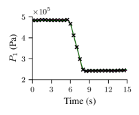
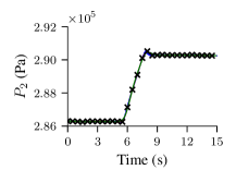
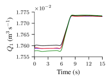
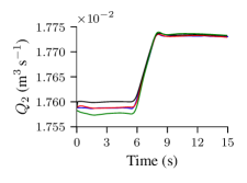
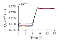
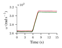
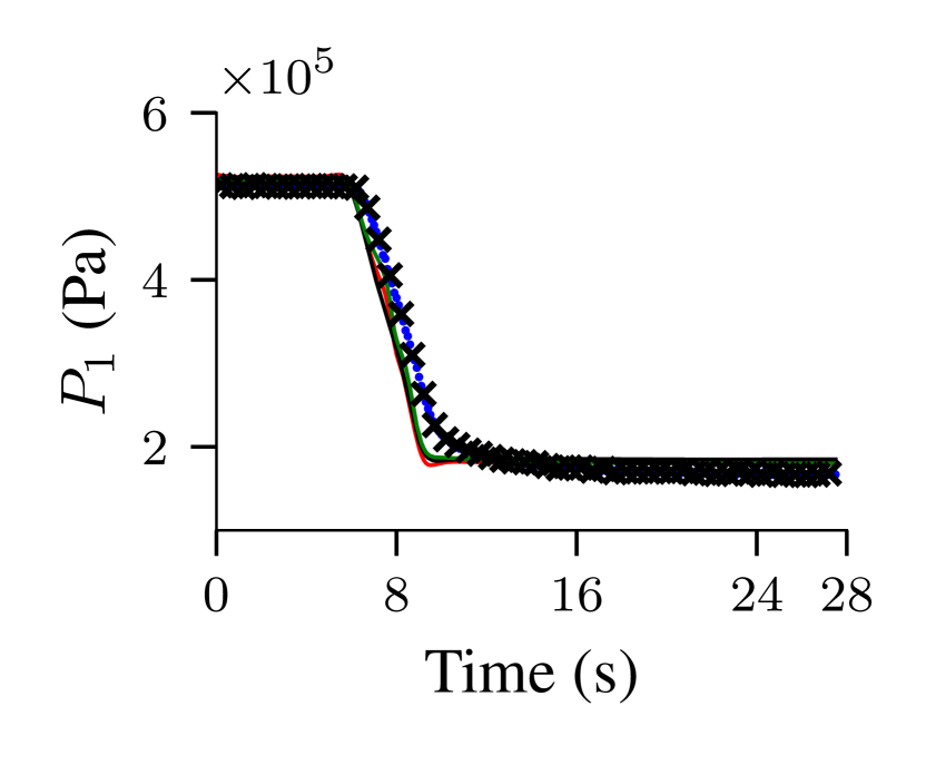
The comparison between the predicted dynamics of the states by the PINN model and the actual values, as shown in Figure 5, demonstrates a good overall agreement across all states and cases. Notably, a small error is observed for the $P_{1}$ and $P_{2}$ states in all cases. However, a slightly larger error is observed for the volumetric flow rate states ($Q_{1}$, $Q_{2}$, and $Q_{p}$) and the ESP angular velocity state ($\omega$). Among the different cases, Case 1 (red line) exhibits the best agreement across the entire simulation range in both investigations. This is also observed in Table 5, where the Case 1 presented the lower MAPE in all states except $P_{1}$.

In the first investigation, the flow rates in Case 2 (black line) and Case 3 (green line) show a reasonable agreement with the simulation approximately from the $6$^th second. However, a slight offset from the actual value is observed from the beginning to the $6$^th second. As for the second investigation (Figure E.1), a slightly higher offset is observed in the flow rate states and in the ESP angular velocity across the entire simulation time for Case 3, while for Case 2, we no longer observe the offset.

4.1.2 State estimation results for simulated data with noise

To further evaluate the robustness of the PINN model, we extend our analysis to include a simulated scenario with Gaussian noise. This section aims to assess the performance of the PINN model when subjected to noise alone without considering missing physics or errors in the model parameter estimation. For each PINN realization, a different noise realization is also considered. Similarly to the previous section, we will focus on presenting the result corresponding to the first experimental investigation, while the result for the second experimental investigation can be found in Appendix E for reference. The MAPE for the different predicted states are shown in Table 6 and the output of the predicted states from the neural network along with the addition of noise on the pressure signals are shown in Figure 6.

Table 6: MAPE for the simulated scenario with added noise. The table presents the MAPE for states prediction in the simulated case with added noise data, considering three cases of unknown parameters. Similarly to Table 5, increasing the number of unknown parameters (Case 1 to Case 3) leads to higher MAPE values for all states, indicating a performance loss. Nevertheless, the MAPE values remain relatively small, and visual inspection of Figure 6 shows a reasonable agreement with the actual values, except for Case 2.

	$P_{1}$	$P_{2}$	$Q_{1}$	$Q_{2}$	$Q_{p}$	$\omega$
Case 1	0.1800004341822363	0.07340612981829478	0.017248754288436006	0.016911218122526037	0.01736920170711386	0.027211784779913383
Case 2	0.16536009954643294	0.020955793953604595	0.4545591272169739	0.45563027952691587	0.45461072011887305	2.814509136183609
Case 3	0.18158854977744587	0.034085485270664746	0.04754425206569738	0.04509845472611995	0.047987541485649356	0.15934479955231245

(a) Intake pressure.

(b) Discharge pressure.

(c) Upstream flow rate.

(d) Downstream flow rate.

(e) Impeller flow rate.

(f) ESP angular velocity.

Fig. 6: Comparison of predicted and true states for the simulated case with noise of the first experimental investigation and unknown parameters. In Figure 6(a) and Figure 6(b), the blue line indicates the signal with added Gaussian noise. In other figures, the same blue line represents the noise-free simulated state. This differentiation aids in evaluating the PINN’s accuracy by comparing its predictions with the actual state values and also present the signal used for PINN training. Each PINN training used a different random seed. Therefore, the Gaussian noise in the signal varied for every PINN training and case. Specifically, the noisy signals for $P_{1}$ and $P_{2}$ in Figure 6(a) and Figure 6(b) correspond to the first training for Case 1, and they were used as a reference. The added Gaussian noise considered the uncertainty from the pressure transducers as specified in Table A.14. For all cases, the training dataset consisted of $37$ data points for data loss in $P_{1}$ and $P_{2}$ and $100$ collocation points for physics loss. The plots show the mean value of results for 30 realization of PINNs. The noisy data shown in the plots are one of noisy data shown as representative sample.

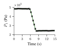
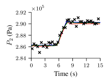
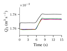
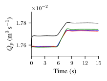
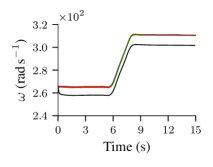
The comparison between the predicted dynamics of the states by the PINN and the actual values, as depicted in Figure 6, demonstrates a good overall agreement all states and investigations for almost all cases. However, in Case 2 (black line), the PINN was unable to accurately estimate the flow rate states ($Q_{1}$, $Q_{2}$ and $Q_{p}$,). They exhibit relatively higher errors, however, the model is able to predict the general shape of the time series. Remarkably, these higher errors were observed exclusively in the first experimental investigation (Figure 7) (higher water cut), whereas in the second investigation (Figure E.3) (with low water cut), Case 2 demonstrated performance similar to that of Case 1 (red line).

Notably, minor errors are observed in the $P_{1}$ and $P_{2}$ states for all cases and investigations. Specifically, in the discharge pressure state (Figure 6(b)), we can observe that the neural network did not overfit and successfully captured the signal trend and magnitude. Similarly to the simulated data without noise (Section 4.1.1), Case 1 (red line) exhibits the best agreement across the entire simulation range in both investigations. Additionally, as shown on Table 6, Case 1 had a lower MAPE than the other cases for the unknown states and a higher MAPE for the known state $P_{2}$.

Despite the addition of noise, the state estimation for the Case 1 and 3 provides good accuracy without significant errors. These results were similar to those obtained in noise-free conditions, with a slight increase in MAPE values. In Case 3, there is a noticeable offset in the volumetric flow rates ($Q_{1}$, $Q_{2}$ and $Q_{p}$) approximately after the $$8$^{\text{th}}$ second, which is different from the observations made in Section 4.1.1, where the offset occurred only in the beginning. Additionally, the angular velocity, in this case, remains closely aligned with the actual values throughout the simulation, exhibiting no offset. It is observed that results for Case 2 deviate from the true values, particularly, for flow rates ($Q_{1}$, $Q_{2}$, $Q_{p}$). It may be possible that, though the Case 2 is structurally identifiable, it is not practical identifiable. However, it is observed that the angular velocity of the ESP ($\omega$) was not significantly affected as that of the flow rates.

4.1.3 State estimation results for experimental data

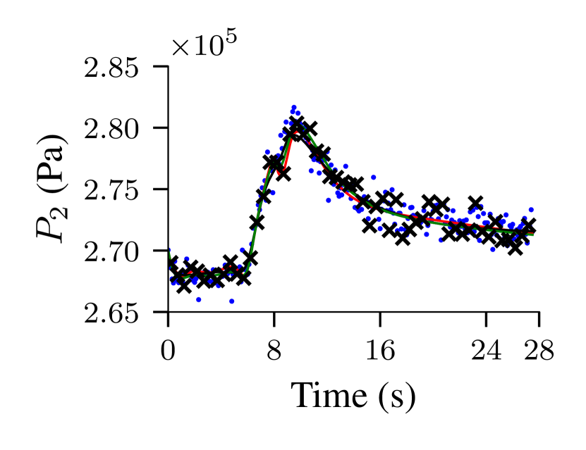
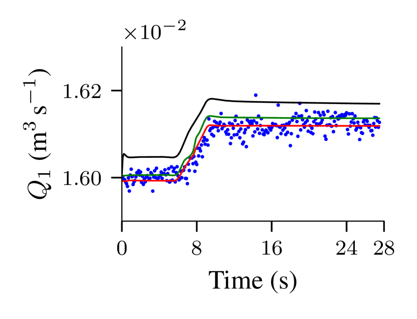
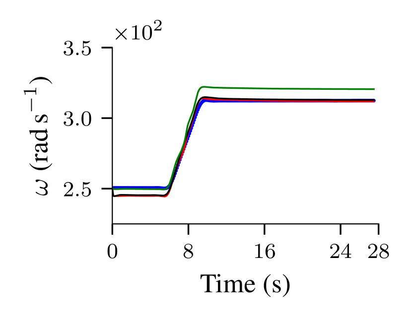
In this section, we assess the performance of the PINN when subjected to experimental data, which is a more representative scenario of real-world oil field conditions. In this case, noise in data and model uncertainties exist, posing a more challenging scenario for the PINN model. Similarly to the previous sections, the results from the first experimental investigation are provided in this section, while results from the second investigation can be found in Appendix E. The MAPE values for these predictions are presented in Table 7. Meanwhile, the predicted outputs of the neural network are shown in Figure 7.

Table 7: MAPE for the experimental data scenario. The table presents the MAPE values for state predictions using experimental data across the three cases with varying unknown parameters. Among the cases evaluated, Case 1 shows the best agreement regarding the upstream volumetric flow rate ($Q_{1}$) and the ESP angular velocity $\omega$. However, similarly to the noisy data scenario, Case 2 presented errors for $\omega$ and $Q_{1}$ that are considerably higher than the other states, as evident in Figures 7(c) and 7(d). Nonetheless, the MAPE values remain relatively small for the other cases and states, and visual inspection of Figure 6 shows a reasonable agreement with the actual values.

	$P_{1}$	$P_{2}$	$Q_{1}$	$\omega$
Case 1	4.517410747974028	0.24518244482745255	0.1367787365669951	1.0648762637051863
Case 2	3.8282224471949213	0.24291714393025327	1.5598161289614378	8.289579011272275
Case 3	2.9626505030357784	0.2517365090066159	0.2182128485083175	1.299768526238012

(a) Intake pressure.

(b) Discharge pressure.

(c) Upstream flow rate.

(d) ESP angular velocity.

Fig. 7: Comparison of predicted and true states for the experimental case of the first experimental investigation with unknown parameters. Due to constraints in our experimental setup, we could only directly measure the states $Q_{1}$, $P_{1}$, $P_{2}$, and $\omega$. Therefore, the PINN results analysis will primarily concentrate on these four states, denoted by the graphs’ blue lines. Moreover, for all cases, the training dataset consists of $48$ data points for data loss with $100$ collocation points for physics loss. The plots show the mean value of results for 30 realization of PINNs.

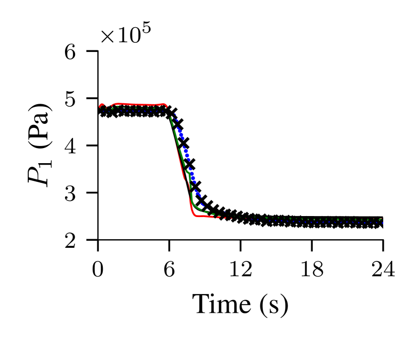
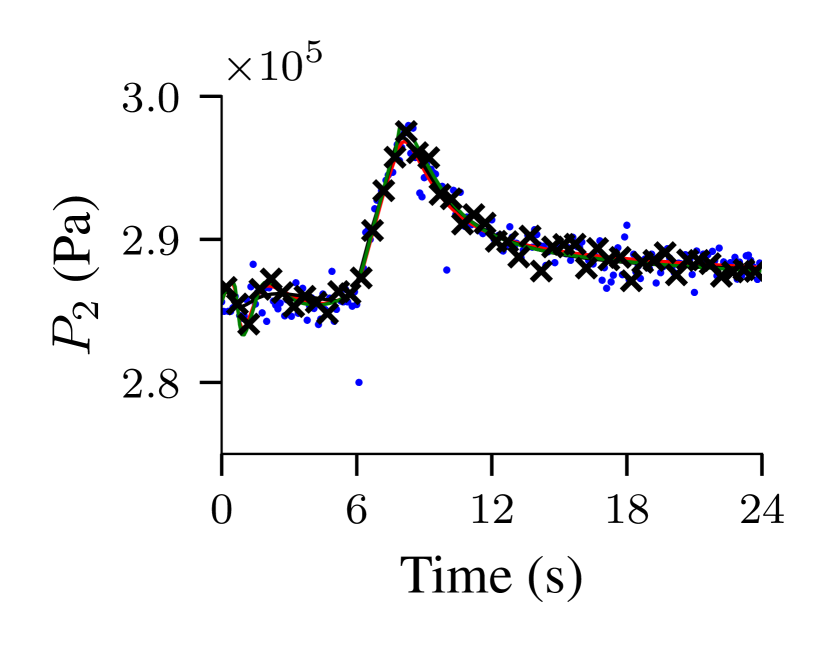
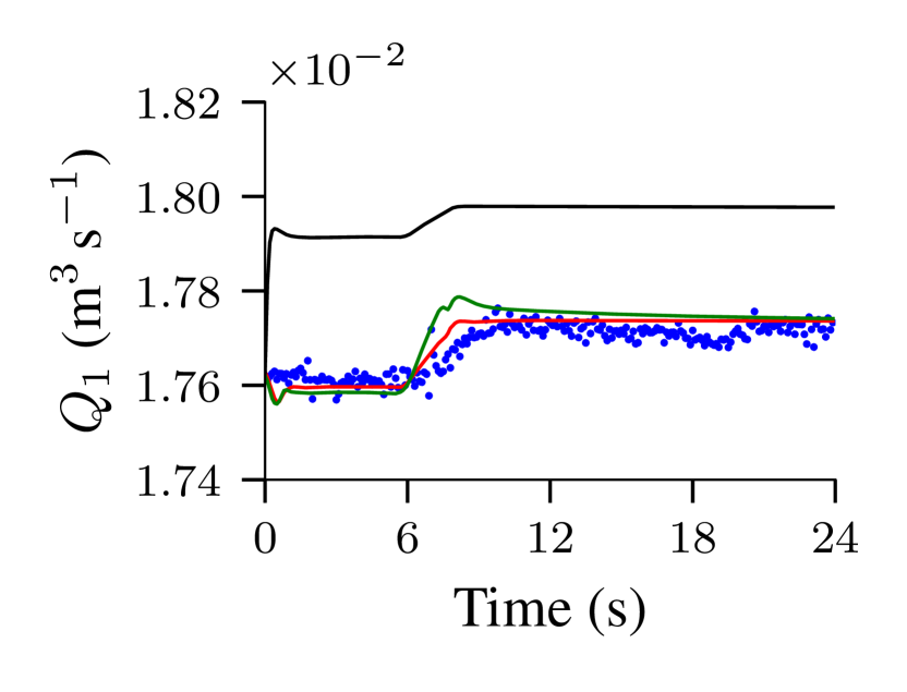
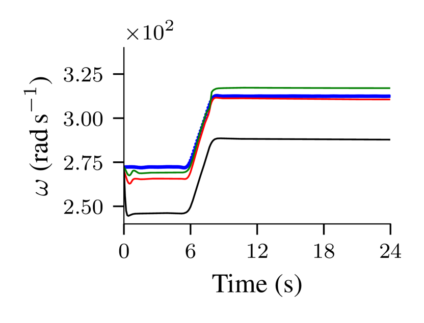
By comparing the PINN-predicted dynamics with the actual values (Figure 7), a good overall agreement is evident across all states and cases, even in the presence of noise and model errors. However, similarly to the noisy data scenario, in Case 2 (black line), the PINN was unable to accurately estimate the flow rate ($Q_{1}$) and angular velocity ($\omega$) states. While the predicted states follow the signal’s shape, they exhibit relatively high errors. Remarkably, these higher errors were observed exclusively in the first experimental investigation (Figure 7) (high water cut), whereas in the second investigation (Figure E.3) (low water cut), Case 2 demonstrated performance similar to that of Case 3 (green line). These high errors are observed in Table 7, where the Case 2 values for $Q_{1}$ and $\omega$ had the highest MAPE values.

Notably, for the $P_{1}$ state (Figure 7(a)), a minor deviation in the PINN prediction’s shape is noticeable when compared to the experimental data. This difference could be attributed to the influence of the fluid’s bulk modulus, which affects the system’s settling time. In the parameter estimation section, we will discuss the challenges encountered in estimating the bulk modulus for the experimental data, as it was not experimentally measured. Furthermore, in the discharge pressure state (Figure 7(b)), it is clear that the neural network did not overfit and successfully captured the signal trend and magnitude, including the signal overshoot between 612, which was considerably smaller in the simulations.

Additionally, a systematic error is noticeable at the beginning of the $\omega$ state (Figure 7(d)) for Cases 1 and 3. Despite these deviations, the predicted $\omega$ signal aligns well with the experimental data regarding shape and magnitude. When comparing the simulated and measured angular velocity ($\omega$), we also observed a systematic error, indicating a difference between the actual and the obtained model parameters. However, the PINN could reasonably estimate the angular velocity state despite this difference. We believe that the observed discrepancies between the experimental data and model predictions could be attributed to multiple factors. These include model uncertainty arising from approximations, simplifications, assumptions in the model, and the influence of noise in the experimental data.

4.2 Parameter estimation results

The results for parameter estimation in the experimental investigations $1$ and $2$ across three cases are presented in the following sections. It should be noted that we did not measure the emulsion bulk modulus during the experiments. As a result, we cannot assess the accuracy of the values determined by the PINN in the experimental data scenario. The viscosity values obtained were compared to the [44] model, described in Section 2.2. For density estimation, we relied on measurements from the Coriolis meter. In this section, we have discussed absolute percentage error, but additional tables presenting actual values can be found in Section 4.3.

In this section, the mean of the absolute percentage error (MAPE) for the parameter estimation results is defined as

$$\text{MAPE}_{\Lambda}=\frac{1}{N^{init}}\sum_{i=1}^{N^{init}}\left|\frac{\Lambda-\hat{\Lambda}_{i}}{\Lambda}\right|,$$ (20)

where $N^{init}$ is the number of PINN random initializations, considered $30$ in this study. The variable $\Lambda$ represents the true value of the unknown parameter, and $\hat{\Lambda}_{i}$ is the estimated unknown parameter for the $i$-th PINN initialization. For simplicity, we refer to the error in this section as the absolute percentage error.

4.2.1 Case 1: Three unknown parameters $B$, $\mu$ and $\rho$ for different types of data

In this section, we focus on Case 1, where we considered the bulk modulus ($B$), viscosity ($\mu$), and density ($\rho$) as unknown while considering the remaining parameters as known. In Table 8, we present the MAPE for the two experimental investigations and all data scenarios.

Table 8: Mean of the absolute percentage error for Case 1.

	Data type	$B$	$\mu$	$\rho$
Investigation 1	Sim.	0.3123914334679205	0.03048262039075415	0.019583041849378462
	Noisy	0.5758474778631687	0.1246478464937965	0.09468425026741538
	Exp.	N/A	1.8022308062573755	0.7958879926832864
Investigation 2	Sim.	0.6118124586223436	0.3155249354959103	0.29123451847482407
	Noisy	0.48019770476369555	0.21430525676055667	0.21391718172044438
	Exp.	N/A	4.302495983974393	2.3983552112728317

As can be seen in Table 8, the PINN could successfully estimate the flow parameters for all cases. In the experimental data scenario, the MAPE were slightly higher, for investigation $1$ the errors were below 2, while investigation $2$ had errors below 4.5. It is important to mention that for the experimental cases, the error refers to the difference between the obtained viscosity and the [44] model, which may be not entirely accurate. Also, we considered the single effective viscosity assumption, as described in Section 2.2. Thus, this higher percentage difference on the can also be related to these assumptions and limitations.

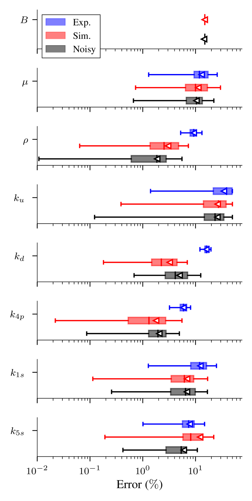
In addition to the mean analysis, it is important to assess the parameter absolute percentage error dispersion. The error dispersion for investigation $1$ and $2$ is visualized in Figure 8(a) and Figure 8(b), respectively.

(a) Investigation 1.

(b) Investigation 2.

Fig. 8: Box plot of the absolute percentage errors for Case 1. Each subfigure shows a specific experimental investigation and contains subplots for each unknown parameter under analysis. Within these subplots, three distinct box plots are presented: blue for the experimental data, red for the simulated data, and gray for the simulated data with added noise. These box plots include whiskers, outliers, and the mean value, represented by a triangle symbol. Outliers are identified as data points that lie more than 1.5 times the interquartile range (IQR) above the third quartile or below the first quartile. The x-axis represents the absolute percentage error, calculated with respect to the reference value. This graphical structure is consistently employed in subsequent figures related to inverse problems.

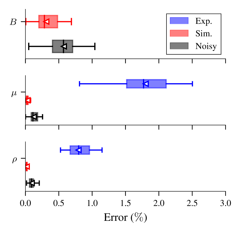
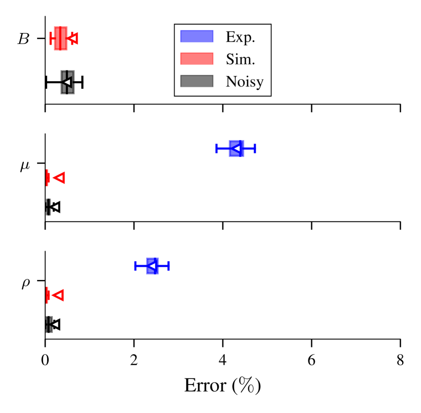
In Figure 8(a) and Figure 8(b), the fluid density ($\rho$) and viscosity ($\mu$) parameters demonstrate consistent behavior across multiple initializations and data sources with relatively low dispersion. On the other hand, Investigation 2 presented outliers in all parameters for the simulated case, and for $\rho$ and $\mu$ in the simulated with noise scenario.

When comparing Investigations 1 and 2 in Table 8 simulated and simulated with noise, we can observe that the performance in Investigation 1 is superior to that in Investigation 2. However, the box plots for both investigations suggest a similar data spread. This discrepancy can be attributed to the influence of outliers on the mean value calculation. As shown in Figure 8(b), the mean value, denoted by a triangle symbol, lies outside the interquartile range, which suggests the impact of outliers. Furthermore, when we compared the median of the errors they presented similar values, which further indicated the influence of these outliers on the mean.

Notably, the addition of noise negatively affected the results, as for most of the parameters, their distributions presented a slightly wider dispersion than the simulated. Further, analyzing the experimental data results, it is evident that they exhibit a wider distribution when compared to the simulated and simulated-with-noise data. This is expected as experimental data is more challenging due to noise and potential model inaccuracies.

4.2.2 Case 2: Seven unknown parameters $B$, $\mu$, $\rho$, $k_{u}$, $k_{d}$, $k_{3p}$ and $k_{4p}$ for different types of data

In this section, we examine Case 2. We treated the fluid’s bulk modulus $B$, viscosity $\mu$, and density $\rho$, along with the pump’s viscous flow loss coefficient $k_{3p}$, the pump equivalent resistance $k_{4p}$, and the equivalent resistances of the upstream and downstream pipeline $k_{u}$ and $k_{d}$ respectively, as unknowns. The remaining parameters were considered known. The MAPE from the two experimental investigations across all data scenarios is provided in Table 9.

Table 9: Mean of the absolute percentage error for Case 2.

		$B$	$\mu$	$\rho$	$k_{u}$	$k_{d}$	$k_{3p}$	$k_{4p}$
Inv. 1	Sim.	2.5213836327651027	13.102961533897538	1.3105662092164572	24.223342389290035	6.151542597588386	4.280495346543093	3.80066181276497
	Noisy	1.3429040186514876	36.42589635565102	5.681855304227679	40.57632313663549	19.066711108882668	9.788220859167755	10.505141326103331
	Exp.	N/A	120.18706717064305	9.718875912541979	77.35400849627332	56.305070224504206	27.67617412905529	29.262093899680988
Inv. 2	Sim.	0.9823345510017082	1.3793030201642582	0.17681157226145608	0.2789054854944502	1.2046161021431807	3.975143325091028	2.2655190369602156
	Noisy	1.2875478059261762	13.0107275452575	3.1028807904373887	3.624120697748016	12.61872000423659	6.44830046649842	6.567684290521311
	Exp.	N/A	14.497828161584577	7.994798599578138	4.8184191577584965	15.393800325496779	9.727351212732747	5.734447186165115

The results presented in Table 9 demonstrate the PINN’s successful estimation of flow parameters across most cases, except for the first investigation’s simulated-with-noise and experimental data scenarios. In these cases, the mean of errors was significantly higher compared to the simulated, simulated and Investigation 2 simulated-with-noise and experimental data scenario. Notably, for the experimental data scenario, the viscosity ($\mu$) exhibited a difference of 120.19, and most other parameters had errors higher than 27. However, for the second investigation, the mean of errors in Table 9 were all below 15.5, indicating better performance in the experimental data scenario. As discussed earlier, the higher error in the experimental case may be caused due to model uncertainty, simplifications in the model, and experimental noise.

However, the results for Investigation 1 in the simulated data scenario require some attention. As shown in Figure 9(a), all unknown parameters presented outliers. Furthermore, their computed means were observed to lie outside the IQR. It was also previously noted in Case 1 (Section 4.2.1), which implies an influence of these outliers on the mean value. When examining the median values illustrated in Figure 9, the error metrics for simulated scenarios in both investigations were predominantly found to be below 1.

(a) Investigation 1.

(b) Investigation 2.

Fig. 9: Box plot of the absolute percentage errors for Case 2. The box plot illustrates the distribution of absolute percentage errors for each parameter in Case 2. Each subplot represents an unknown parameter for the data scenarios evaluated. The x-axis has been changed to logarithmic for better visibility. This graphical structure is consistently employed in subsequent figures related to inverse problems.

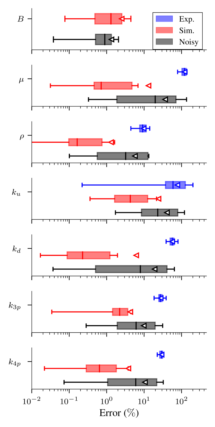
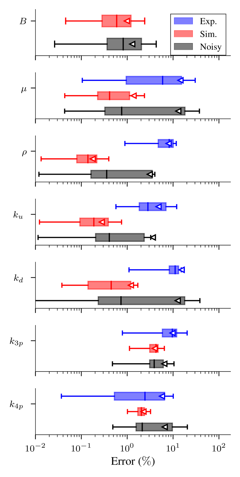
The addition of noise considerably affected the results in both experimental investigations, leading to higher mean errors as shown in Table 9, whereas in investigation, the mean of the errors was smaller than in experimental Investigation 1. Analyzing the box plots in Figure 9, we can observe that the simulated noisy scenario resulted in greater dispersion for most parameters. This observation indicates that the introduction of noise adversely affected the accuracy of the estimated parameters. Moreover, we can observe that similar to the discussed in Section 4.2.1, the experimental data scenario presented the highest mean errors across the initializations for both experimental investigations, except for the $k_{4p}$ in the second experimental investigation.

Despite the high errors in Investigation 1’s experimental data scenario, most estimated parameters exhibited relatively small dispersion across the weight initializations, as evident in Figure 9(a). It is worth noting that the parameter selection for this case did not consider the practical identifiability analysis, which assessed, in this study, the parameter sensitivity to noise. Therefore, this higher mean error with relatively low dispersion suggests that the system might not be practically identifiable within the flow condition of experimental investigation 1. It is possibly converging to a parameter set other than the true one. It is important to note that as the water cuts increase up to the emulsion phase inversion, the fluid behavior becomes more complex, posing a more challenging scenario than lower water cuts. Further, in our practical identifiability analysis, we considered only the sensitivity analysis rather than the Monte Carlo approach, where the optimization algorithm, in this case, the PINN, would be also included.

Therefore, to draw more definitive conclusions about how the parameter estimation is sensitive to the water cut, additional investigations need to be conducted with a larger experimental test matrix that covers a wider range of water cuts. Additionally, a Monte Carlo approach with the PINN on the practical identifiability analysis could potentially better evaluate the effects of the model uncertainties with the experimental data scenario, as the approach described in Section 3.2 considered only the simulated data. Further, as the local structurally identifiability analysis assesses the identifiability of the neighborhood of the parameter set, it is possible that restricting the search range and imposing stricter bounds on the parameter search could lead to better results. This approach is suggested in [49].

4.2.3 Case 3: Eight unknown parameters $B$, $\mu$, $\rho$, $k_{u}$, $k_{d}$, $k_{4p}$, $k_{1s}$ and $k_{5s}$ for different types of data

In this section, we present the results of the inverse problem for Case 3, specifically evaluating the performance of the parameter estimation. The evaluation is based on the MAPE, as shown in Table 10. The considered parameters, in this case, include the bulk modulus ($B$), viscosity ($\mu$), and density ($\rho$) of the fluid, as well as the pump equivalent resistance ($k_{4p}$), the first impeller-fluid coupling coefficient ($k_{1s}$), the shaft second-order friction coefficient ($k_{5s}$), and the equivalent resistance of the pipeline upstream and downstream ($k_{u}$ and $k_{d}$).

Table 10: Mean absolute percentage error for Case 3.

		$B$	$\mu$	$\rho$	$k_{u}$	$k_{d}$	$k_{4p}$	$k_{1s}$	$k_{5s}$
Inv. 1	Sim.	14.948393812003523	11.30713490641263	3.024805096842582	26.265713080933235	3.245079950345309	1.7870117025733798	6.915994745528416	12.238812343580294
	Noisy	14.506395405134993	10.410154579252954	1.876820470788757	25.968600096706027	4.988127891202737	2.0572638224050976	6.87848107572102	6.000178140461784
	Exp.	N/A	13.052403078428918	9.25517303301117	34.50834145300853	16.00668914180382	5.87474192124567	12.368655917350498	7.759101924557011
Inv. 2	Sim.	14.99912943614503	14.336275224657458	4.119317099646765	6.900439504079831	6.655014737929068	3.428187328070186	12.70645447894859	6.9644067851452105
	Noisy	14.999787155925478	13.658673159887488	3.7653651802310963	4.91554888888324	13.634281233475127	7.0420931764339505	11.863419587322072	12.215725252776759
	Exp.	N/A	1.5967748423505708	10.158213110725832	1.9600652119559312	12.052400641918984	5.281842999816811	7.00733773341248	9.246945308406612

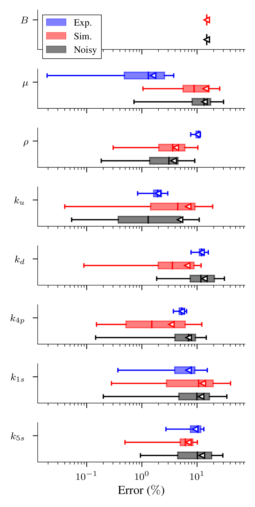
The results in Table 10 and Figure 10 indicate that the PINN successfully estimated the density and viscosity for all scenarios in Case 3, but it encountered challenges in estimating the bulk modulus. The 15 value represents the upper and lower bounds imposed on the output scaling transformation for the bulk modulus. Additionally, when analyzing the dispersion in Figure 10, it is evident that the distributions of the simulated with added noise case are similar to those of the simulated case, with similar IQR.

In Table 10, the distinction between data sources with smaller errors, as observed in Cases 1 and 2 (Section 4.2.1 and Section 4.2.2), is not evident. The Investigation 1 and 2 demonstrated errors mostly below 13. Notably, in Investigation 1, the upstream pipeline equivalent resistance ($k_{u}$) exhibited the highest errors across all data sources, reaching up to 34.51. However, in Figure 3(b), we can observe that the $k_{u}$ presented a relatively high correlation with other parameters, such as the $k_{d}$. On the other hand, in Investigation 2, we do not observe errors as high as in Investigation 1. This discrepancy can likely be attributed to the distinct flow characteristics of each investigation. As previously discussed in Section 4.2.2, further tests under diverse flow conditions are essential to understand the performance difference between Investigation 1 and 2 comprehensively.

It is noteworthy that, for Case 3, besides the fluid bulk modulus and density, the other parameters also have bounded output scaling transformations, which could have contributed to lower errors. Thus, although Case 3 poses an additional challenge compared to Case 2, once it involves estimating eight unknown parameters instead of seven, Case 3 and Case 2 are not directly comparable.

(a) Investigation 1.

(b) Investigation 2.

Fig. 10: Box plot of the absolute percentage errors for Case 3. The box plot illustrates the distribution of absolute percentage errors of each parameter in Case 3. The individual subplots correspond to the unknown parameters across the evaluated data scenarios. To enhance visibility, the x-axis has been changed to a logarithmic scale.

4.3 Estimated unknown parameters mean and standard deviation

In this section, we present additional PINN results for parameter estimation in the ESP system model. These results are obtained by averaging parameter estimations over the PINN 30 training runs and computing the standard deviation. The tables Tables 11 and 12 contain the results of the first and second experimental investigations, respectively. It is important to note that these tables serve as complementary results of the discussed in Section 4.2 and are not the focus of detailed discussion in this work. They are included for the sake of completeness and may be of interest to future research works. Any parameter not accounted for in a specific case is denoted by the symbol.

For each of the three cases, defined based on varying assumptions regarding known parameters, the table presents the performance of PINN in estimating the unknown parameters across the three data scenarios. We average each parameter estimation over the 30 weight initializations , and the standard deviation is indicated by the symbol $\pm$. Parameters not considered in a given case are denoted by the $-$ symbol.

Table 11: Estimation results of ESP system model parameters using PINN for Investigation 1. For each of the three cases, defined based on varying assumptions regarding known parameters, the table presents the performance of PINN in estimating the unknown parameters across the three data scenarios. Each parameter estimation is averaged over 30 training runs to account for the impact of neural network weight initialization. Furthermore, the standard deviation is presented after the $\pm$. The parameters not considered in the case were left blank.

Parameter True Investigation 1 Case 1 Case 2 Case 3 Simulated Simulated with noise Experimental data Simulated Simulated with noise Experimental data Simulated Simulated with noise Exp $B$ $1.31109$ $1\,305\,537\,715.810\,572\,1$ $\pm$ $6\,834\,363.590\,726\,812$ $1\,305\,912\,431.090\,448$ $\pm$ $2\,494\,092.926\,936\,567$ N/A $1\,290\,807\,096.491\,532\,3$ $\pm$ $6\,250\,216.640\,132\,566$ $1\,335\,169\,614.256\,528$ $\pm$ $60\,427\,457.483\,783\,044$ N/A $1\,113\,528\,012.299\,512$ $\pm$ $1417.426\,091\,866\,071\,8$ $1\,114\,176\,041.062\,753\,4$ $\pm$ $1\,791\,954.962\,794\,172\,3$ N/A $\mu$ $0.142\,936\,283\,569\,257\,67$ $0.145\,512\,325\,305\,062\,2$ $\pm$ $0.000\,563\,340\,727\,475\,889\,5$ $0.142\,973\,844\,254\,230\,93$ $\pm$ $3.796\,144\,904\,147\,34510-05$ $0.142\,923\,330\,516\,450\,8$ $\pm$ $0.000\,206\,865\,730\,146\,454\,15$ $0.314\,727\,210\,713\,862\,1$ $\pm$ $0.040\,749\,770\,009\,304\,895$ $0.161\,163\,703\,643\,674\,88$ $\pm$ $0.038\,455\,748\,664\,932\,364$ $0.194\,236\,146\,674\,180\,93$ $\pm$ $0.056\,105\,981\,121\,755\,1$ $0.124\,279\,663\,692\,472\,02$ $\pm$ $0.009\,013\,498\,578\,754\,837$ $0.127\,377\,114\,951\,386\,95$ $\pm$ $0.011\,143\,517\,528\,427\,245$ $0.128\,119\,833\,529\,749$ $\pm$ $0.007\,775\,969\,378\,067\,058$ $\rho$ $882.205\,301\,549\,905\,9$ $875.183\,935\,484\,054\,7$ $\pm$ $1.810\,509\,679\,409\,541\,2$ $882.041\,999\,975\,823\,8$ $\pm$ $0.123\,811\,023\,912\,427\,49$ $882.210\,599\,579\,658\,7$ $\pm$ $0.951\,800\,208\,563\,863\,3$ $936.668\,853\,162\,035\,5$ $\pm$ $73.044\,654\,988\,061\,81$ $891.503\,985\,417\,589\,4$ $\pm$ $24.580\,366\,667\,558\,03$ $927.363\,549\,248\,764\,2$ $\pm$ $53.329\,393\,177\,515\,8$ $800.555\,674\,385\,064\,3$ $\pm$ $18.382\,949\,317\,609\,302$ $906.444\,372\,451\,502\,5$ $\pm$ $21.190\,948\,393\,945\,5$ $879.809\,816\,868\,559$ $\pm$ $20.538\,046\,874\,756\,947$ $k_{u}$ $51.024\,099\,349\,975\,586$ $21.533\,104\,565\,956\,37$ $\pm$ $38.605\,403\,296\,553\,24$ $59.980\,880\,290\,939\,78$ $\pm$ $25.707\,810\,628\,383\,672$ $50.762\,289\,619\,915\,19$ $\pm$ $29.085\,180\,979\,234\,867$ $36.699\,570\,991\,693\,996$ $\pm$ $12.953\,893\,714\,252\,207$ $39.234\,978\,970\,307\,72$ $\pm$ $10.130\,686\,775\,300\,914$ $40.023\,161\,022\,846\,56$ $\pm$ $10.287\,044\,038\,386\,886$ $k_{d}$ $30.669\,759\,377\,918\,858$ $13.401\,129\,822\,495\,175$ $\pm$ $3.211\,508\,532\,929\,21$ $28.799\,304\,945\,343\,565$ $\pm$ $4.001\,276\,545\,963\,861$ $24.836\,430\,766\,321\,15$ $\pm$ $6.258\,850\,209\,258\,602$ $35.578\,972\,422\,081\,556$ $\pm$ $0.606\,049\,320\,732\,410\,2$ $31.240\,421\,511\,035\,54$ $\pm$ $1.162\,120\,945\,163\,466\,6$ $32.094\,014\,953\,196\,58$ $\pm$ $1.082\,791\,489\,899\,441\,7$ $k_{3p}$ $-63\,059\,695.623$ $-45\,607\,184.457\,794\,376$ $\pm$ $3\,029\,168.941\,973\,645$ $-62\,330\,730.513\,838\,53$ $\pm$ $4\,254\,117.321\,108\,799$ $-58\,144\,916.801\,469\,24$ $\pm$ $6\,830\,749.171\,367\,95$ $k_{4p}$ $-2\,227\,387.757$ $-1\,937\,460.863\,517\,610\,8$ $\pm$ $119\,279.618\,650\,855\,12$ $-2\,635\,020.818\,512\,129\,6$ $\pm$ $194\,213.764\,727\,131\,2$ $-2\,451\,957.977\,854\,705\,4$ $\pm$ $284\,197.017\,118\,707\,07$ $-2\,899\,833.769\,698\,137\,4$ $\pm$ $32\,167.241\,919\,486\,25$ $-2\,776\,041.450\,402\,519\,7$ $\pm$ $55\,998.770\,864\,629\,21$ $-2\,788\,488.095\,825\,981\,3$ $\pm$ $42\,754.105\,307\,946\,36$ $k_{1s}$ $-61.260\,783\,417\,128\,89$ $-53.735\,749\,920\,157\,87$ $\pm$ $3.773\,670\,110\,030\,255$ $-64.259\,425\,552\,440\,26$ $\pm$ $4.058\,014\,789\,557\,102$ $-58.680\,531\,114\,414\,364$ $\pm$ $4.259\,711\,769\,599\,78$ $k_{5s}$ $0.000\,142\,303\,446\,685\,515\,65$ $0.000\,131\,261\,977\,215\,028\,82$ $\pm$ $5.045\,320\,945\,214\,9710-06$ $0.000\,159\,021\,853\,114\,132\,3$ $\pm$ $1.636\,140\,313\,474\,549\,310-05$ $0.000\,142\,046\,828\,696\,298\,76$ $\pm$ $1.119\,658\,458\,598\,804\,910-05$

Table 12: Estimation results of ESP system model Parameters using PINN for Investigation 2. The table presents the performance of PINN in estimating unknown parameters across three distinct cases different set of known parameters. The estimations are derived from the average over the 30 trainings to consider neural network weight initialization effects. The standard deviations are indicated by the values following the $\pm$ symbol. The symbol denotes parameters not considered in the case.

Parameter True Investigation 2 Case 1 Case 2 Case 3 Simulated Simulated with noise Experimental data Simulated Simulated with noise Experimental data Simulated Simulated with noise Exp $B$ $1\,310\,000\,000.0$ $1\,321\,642\,556.826\,588\,6$ $\pm$ $71\,980\,883.334\,832\,15$ $1\,309\,474\,919.688\,656\,3$ $\pm$ $16\,993\,678.862\,998\,623$ N/A $1\,292\,723\,670.897\,588$ $\pm$ $7\,891\,846.136\,213\,479$ $1\,318\,493\,936.050\,693\,5$ $\pm$ $18\,224\,981.342\,153\,12$ N/A $1\,113\,528\,276.927\,492\,1$ $\pm$ $1295.758\,260\,428\,117\,4$ $1\,113\,511\,404.386\,500\,1$ $\pm$ $51\,856.787\,849\,898\,72$ N/A $\mu$ $0.228\,118\,012\,154\,712\,25$ $0.237\,932\,780\,466\,391$ $\pm$ $0.000\,584\,067\,102\,253\,053\,4$ $0.228\,811\,636\,766\,471$ $\pm$ $0.002\,986\,289\,178\,406\,977$ $0.228\,433\,922\,385\,898\,8$ $\pm$ $0.001\,404\,682\,632\,730\,578\,2$ $0.246\,845\,314\,711\,347\,44$ $\pm$ $0.054\,298\,229\,041\,233\,1$ $0.231\,151\,814\,264\,013\,07$ $\pm$ $0.005\,619\,878\,131\,403\,726\,5$ $0.257\,318\,569\,645\,328\,1$ $\pm$ $0.054\,333\,646\,920\,332\,86$ $0.228\,830\,814\,335\,275\,5$ $\pm$ $0.004\,505\,004\,222\,817\,441\,5$ $0.195\,573\,978\,836\,794\,42$ $\pm$ $0.032\,264\,539\,608\,416\,71$ $0.257\,192\,788\,848\,514\,2$ $\pm$ $0.021\,157\,935\,501\,196\,767$ $\rho$ $872.591\,135\,484\,436\,9$ $851.663\,300\,513\,441$ $\pm$ $1.911\,033\,821\,280\,820\,4$ $870.112\,849\,811\,701\,5$ $\pm$ $10.368\,572\,462\,967\,753$ $871.449\,785\,551\,229\,6$ $\pm$ $5.205\,244\,913\,363\,277$ $828.667\,380\,215\,241\,6$ $\pm$ $69.757\,449\,758\,875\,74$ $872.729\,097\,117\,052\,9$ $\pm$ $1.965\,339\,862\,672\,919\,3$ $899.254\,463\,315\,760\,2$ $\pm$ $42.538\,655\,075\,884\,876$ $783.951\,468\,356\,625\,2$ $\pm$ $10.753\,435\,077\,964\,234$ $906.923\,872\,830\,932\,7$ $\pm$ $26.446\,110\,799\,709\,885$ $894.414\,297\,892\,856\,4$ $\pm$ $35.981\,859\,096\,924\,23$ $k_{u}$ $656.553\,858\,757\,019$ $629.050\,433\,511\,714\,2$ $\pm$ $32.060\,947\,271\,356\,73$ $658.014\,394\,347\,284\,1$ $\pm$ $2.058\,807\,333\,233\,073$ $661.641\,438\,037\,221$ $\pm$ $51.118\,161\,499\,645\,61$ $643.684\,974\,973\,768\,6$ $\pm$ $3.447\,031\,568\,011\,228\,7$ $626.199\,681\,813\,715\,5$ $\pm$ $61.916\,280\,857\,671\,325$ $655.079\,089\,366\,513$ $\pm$ $64.102\,190\,883\,234\,68$ $k_{d}$ $27.025\,931\,881\,022\,082$ $26.663\,098\,405\,819\,97$ $\pm$ $5.721\,633\,038\,425\,67$ $26.728\,532\,118\,188\,74$ $\pm$ $0.585\,876\,654\,245\,717\,3$ $23.637\,526\,849\,961\,777$ $\pm$ $5.914\,879\,947\,856\,169$ $30.283\,205\,468\,534\,966$ $\pm$ $0.538\,041\,086\,852\,687\,1$ $28.677\,475\,141\,804\,525$ $\pm$ $2.158\,320\,534\,289\,664$ $23.511\,647\,465\,320\,82$ $\pm$ $2.421\,691\,830\,892\,320\,3$ $k_{3p}$ $-63\,059\,695.623$ $-65\,847\,939.076\,599\,516$ $\pm$ $6\,582\,827.981\,397\,631$ $-65\,566\,408.905\,340\,93$ $\pm$ $786\,588.887\,548\,278\,3$ $-62\,349\,257.660\,900\,71$ $\pm$ $5\,679\,663.396\,466\,728$ $k_{4p}$ $-2\,227\,387.757$ $-2\,639\,722.162\,085\,309\,6$ $\pm$ $247\,175.942\,651\,153\,45$ $-2\,676\,877.820\,125\,957$ $\pm$ $33\,482.442\,964\,229\,72$ $-2\,559\,044.578\,139\,134\,7$ $\pm$ $233\,765.040\,091\,121\,45$ $-2\,883\,594.690\,545\,000\,6$ $\pm$ $24\,036.241\,458\,571\,57$ $-2\,729\,588.690\,568\,007\,5$ $\pm$ $132\,608.198\,973\,589\,84$ $-2\,546\,050.856\,661\,753\,3$ $\pm$ $107\,733.293\,613\,855\,17$ $k_{1s}$ $-61.260\,783\,417\,128\,89$ $-57.159\,073\,898\,237\,65$ $\pm$ $2.383\,592\,865\,231\,957\,3$ $-54.731\,328\,869\,272\,48$ $\pm$ $7.901\,564\,077\,637\,516$ $-65.125\,035\,791\,906\,65$ $\pm$ $8.288\,111\,281\,042\,976$ $k_{5s}$ $0.000\,142\,303\,446\,685\,515\,6$ $0.000\,129\,144\,724\,798\,528\,44$ $\pm$ $4.276\,273\,232\,409\,82310-06$ $0.000\,147\,921\,968\,733\,183\,1$ $\pm$ $9.842\,989\,696\,981\,21310-06$ $0.000\,149\,288\,937\,021\,130\,96$ $\pm$ $2.034\,338\,173\,734\,12610-05$

5 Summary

In this study, our primary focus was on developing a physics-informed neural network (PINN) model in order to estimate unknown states and parameters of the electrical submersible pump (ESP) system operating in a two-phase flow condition when only limited state variables are known. In the present study, we only know the pump intake and discharge pressure states measurements. The PINN model may reduce the field laboratory test required to estimate the fluid properties. We first investigated the structural and practical identifiability of the ESP system, defining three distinct sets of unknown parameters. Subsequently, we assessed the performance of the PINN model on these parameter sets across two experimental studies (water to oil ratio) encompassing three data scenarios: simulated, simulated with added noise, and experimental data.

We conducted a local structural identifiability analysis using the differential elimination method for dynamical models via projections, as proposed by [23]. The results revealed that the system is not locally structurally identifiable when both intake and discharge pressures are the only known parameters. For local structural identifiability, we had to consider the parameters like shaft inertia ($I_{s}$), fluid-impeller disk friction ($k_{3s}$), and shaft viscous damping ($k_{4s}$) as known, resulting in $12$ identifiable unknown parameters. Then, we derived the parameter correlation matrix using the Fisher information matrix for the practical identifiability analysis. Practical identifiability provides a qualitative analysis for the unknown parameters in the presence of noise. To attain this identifiability, it became necessary to define more parameters as known. Thus, we selected the most critical parameters in the context of the ESP’s actual operation as unknown and other parameters as known. These unknown parameters included the fluid properties and pipeline equivalent resistance.

The proposed PINN model in this study successfully estimated the ESP’s fluid properties (bulk modulus, density, and viscosity) and dynamics of the states with reasonable accuracy. In the case when we considered fluid properties, pipeline equivalent resistances, shaft, and pump parameters, the model provides a reasonable accuracy when considering simulated data with low water cut. However, we observed a relatively higher error for higher water cut or when we considered simulated with noise and experimental data with lower water cut.

In this case, we observed outliers in the predicted results. Further study may include a robust PINN method to eliminate the outliers and better performance. Furthermore, we also observed that errors are higher in the case of higher water cuts. This error is higher in the case of noise and experimental data than in the simulated cases. These cases with more unknowns may require additional measurements of the state variables, which are generally not measured in the field. Future studies may also include further investigations with a broader range of water fractions to understand better the water cut influences. The study may also focus on updating the numerical model for higher water cuts if necessary, as assumptions made on the numerical model may not be valid for higher water cuts.

Obtaining the estimated parameters and states for the ESP system in oil production can be challenging, and the PINN offers a promising and cost-efficient alternative for estimating them. Although this approach has its benefits, it also has some limitations. One of the limitations is that the technique is computationally intensive. This means that for every desired estimation of properties, the PINN must undergo training. More efficient PINN algorithms need to be investigated for different operational conditions. Furthermore, the accuracy of the estimated properties using PINN is heavily reliant on the accuracy of the measured states and known parameters. In the event of a faulty reading or instrument failure, the PINN’s ability to provide accurate estimations is compromised.

Additionally, a Monte Carlo approach with the PINN on the practical identifiability analysis could potentially better evaluate the effects of the model uncertainties with the experimental data scenario. As the experimental data contains noise, further study may also include uncertainty quantification study. Furthermore, an ESP system model that considers the multistage separately would be relevant for ESPs in actual production, whose number of stages are considerably higher than the one considered in this study. Moreover, the current model does not consider the electrical domain, and its inclusion would be more realistic. Another notable aspect is the single viscosity assumption for the system, highlighted in Section 2.2, which remains a limitation.

Appendix A Experimental procedure

A.1 Fluid characterization

The oil viscosity measurement used a rotational rheometer model HAAKE MARS III. The measurements ranged from $10\text{\,}\mathrm{\SIUnitSymbolCelsius}60\text{\,}\mathrm{\SIUnitSymbolCelsius}$ with a step of approximately $0.5\text{\,}\mathrm{\SIUnitSymbolCelsius}$. For each temperature, the oil viscosity was measured three times. The Figure A.11 shows the measured viscosity as a function of the temperature. Then, using least squares, we obtained a 4^th order polynomial, Equation 21, that fits viscosity measurements to the temperature.

$$\mu(T)=\frac{$0.000\,264\,36$\,T^{4}-$0.048\,64$\,T^{3}+$3.436$\,T^{2}-$114.28$\,T+$1610.3$}{$1000$}$$ (21)

Fig. A.11: The oil viscosity for a temperature range of $10\text{\,}\mathrm{\SIUnitSymbolCelsius}60\text{\,}\mathrm{\SIUnitSymbolCelsius}$.

A.2 Experimental apparatus

The equipments specifications are presented in Table A.13, and the instrumentation characteristics are shown in Table A.14.

Table A.13: Experimental setup components specification. The component’s specifications are separated by the flow line where they are installed.

Line	Device	Model
Oil	Pump	NETZSCH two-screw pump
	Motor	WEG, $45\text{\,}\mathrm{kW}$, 1775RPM
	VSD-1	CFW 700 WEG Vectrue inverter
Water	Pump	IMBIL 65160
	Motor	WEG, $22\text{\,}\mathrm{kW}$, 3535RPM
	VSD-2	CFW 700 WEG Vectrue inverter
Emulsion	Pump	Baker Hughes P100L 538 series
	Motor	WEG, $37\text{\,}\mathrm{kW}$, 3555RPM
	VSD-3	CFW 09 WEG Vectrue inverter
	Tank	Intelfibra, capacity 12000
Heat control	Heat exchanger	FYTERM T3480 shell and tube
	Heater	Mecalor TMR-M-18-380/C
	Chiller	Mecalor MSA-60-CA-380/C
Valve	Choke	Fisher 657 glob valve

Table A.14: Instrumentation range and uncertainty.

Instrument	Model	Range	Uncertainty
Flow meters	Micro Motion®F300S355	$0100\text{\,}{\mathrm{m}}^{3}\text{\,}{\mathrm{h}}^{-1}$	0.2 O.V.*
Temperature sensors	ECIL®PT100	$0100\text{\,}\mathrm{\SIUnitSymbolCelsius}$	1/10 DIN
Pressure transducers	Emerson Rosemount 2088	$0200\text{\,}\mathrm{kPa}$	0.065 F.S.*
Water cut meter	Roxar Nemko 05 ATEX 112	$0100\text{\,}\mathrm{\char 37\relax}$	1 F.S.
Torque transmitter	HBM T21WN	$0100\text{\,}\mathrm{N}\text{\,}\mathrm{m}$	0.1 F.S.
Encoder	Minipa MDT-2238A	$0166\text{\,}\mathrm{Hz}$	0.05F.S.

• *O.V. : of value; F.S. : of full scale.

Appendix B Electrical submersible pump system model

We relied on experimental data collected under steady-state conditions to determine the parameters for the ESP model. The equivalent resistance for the pipelines and constants associated with the twin-screw pump was obtained from this data. Notably, due to the experimental setup’s constraints related to temperature control, we used the heat exchanger bypass valve for fine temperature control. The valve is depicted in Figure 1. Consequently, it became necessary to individually distinguish the equivalent resistance of the upstream pipeline and the twin-screw pump parameters for both experimental investigations 1 and 2. Therefore, the Table B.1 presents the parameters that are constant for both experimental investigations and Table B.2 presents the parameters that change with the experimental investigation.

Table B.1: Parameters for the ESP model. The table presents the parameters used in the ESP model, including the impeller, shaft, oil pump, and pipeline coefficients. They were obtained using steady-state conditions, while fluid parameters varied based on the specific investigation conducted. Geometrical parameters, such as pipeline diameter, length, and cross-sectional area, were directly measured from the experimental setup.

#	Description	Symbol	Value	Unit
1	1st impeller-fluid coupling and shock loss coefficient	$k_{1p}$	$4.867\,670\,280\,64$
2	2nd impeller-fluid coupling and shock loss coefficient	$k_{2p}$	$0.009\,930\,005\,71$
3	Pump viscous flow loss coefficient	$k_{3p}$	$-63\,059\,695.623$∗
4	Pump equivalent resistance	$k_{4p}$	$-2\,227\,387.757$∗	4
5	Shaft 1st impeller-fluid coupling coefficient	$k_{1s}$	$-61.260\,783\,417\,128\,89$∗	□
6	Shaft 2nd impeller-fluid coupling coefficient	$k_{2s}$	$0.007\,812\,519\,509\,782\,526$
7	Fluid-impeller disk friction constant	$k_{3s}$	$0.110\,371\,603\,455\,165\,95$	2
8	Shaft viscous damping coefficient	$k_{4s}$	$0.067\,320\,528\,257\,952\,3$
9	Shaft second-order friction coefficient	$k_{5s}$	$0.000\,142\,303\,446\,685\,515\,65$
10	Shaft moment of inertia	$I_{s}$	$0.000\,508\,450\,865\,750\,310\,8$	2
11	Fluid bulk modulus	$B$	$1.31109$
12	Downstream pipeline diameter	$d_{d}$	$0.0762$
13	Downstream pipeline cross-sectional area	$A_{d}$	$0.004\,560\,367\,311\,877\,479$	□
14	Downstream pipeline length	$L_{d}$	$28$
15	Upstream pipeline diameter	$d_{u}$	$0.0762$
16	Upstream pipeline cross-sectional area	$A_{u}$	$0.004\,560\,367\,311\,877\,479$	□
17	Upstream pipeline length	$L_{u}$	$31.5$
18	Cross-sectional area of all impeller channels†	$A_{p}$	$0.004\,896\,564\,849\,701\,392$	□
19	Impeller channel length‡	$L_{p}$	$0.0475$

• The negative sign indicates that the obtained parameter is opposite in sign to what is considered in the equations.

• The ESP P100L has a mixed impeller whose channel height varies from the inlet to the outlet. In this study, we assume a linear variation in channel height and approximate it using its arithmetic mean, obtained by the impeller inlet and outlet heights.

• We approximate the channel length as the difference between the inner and outer diameters of the impeller.

Table B.2: Parameters for the twin-screw pump and pipeline. It is important to mention that the value of the downstream equivalent resistance ($k_{d}$) provided takes into account the losses from the valve, as depicted in the experimental setup schematics in Figure 1. Additionally, the values for the pipeline equivalent resistances ($k_{u}$ and $k_{d}$) also reflect manual fine-tuning adjustments made to the model.

#	Description	Symbol	Inv. 1	Inv. 2	Unit
20	Fluid effective viscosity	$\mu$	$0.142\,936\,283\,569\,257\,67$	$0.228\,118\,012\,154\,712\,25$
21	Fluid density	$\rho$	$882.205\,301\,549\,905\,9$	$872.591\,135\,484\,436\,9$
22	Upstream pipeline resistance coefficient	$k_{u}$	$51.024\,099\,349\,975\,586$	$656.553\,858\,757\,019$	1
23	Downstream pipeline resistance coefficient	$k_{d}$	$30.669\,759\,377\,918\,858$	$27.025\,931\,881\,022\,082$	1
24	Twin-screw pump angular velocity	$\omega_{t}$	$1280.0$	$1160.0$	RPM
25	Twin-screw pump flow-rate coefficient	$k_{bd}$	$162\,186.577\,144\,296\,26$	$133\,454.746\,196\,686\,55$
26	Twin-screw pump leaking coefficient	$k_{bl}$	$1.144\,146\,250\,765\,159\,61010$	$9.564\,585\,432\,214\,49109$

Fig. B.1: Bond graph model of the ESP system. It is crucial to emphasize that the terms in the shock loss and the GY expression overlap. Consequently, their individual contributions cannot be isolated while obtaining them experimentally.

Appendix C Detail physics loss function for the PINN model for the ESP system

As presented in Section 2.3, the PINN physics loss function for the ESP system is defined as

$$\mathcal{L}^{ode}(\bm{\theta},\bm{\Lambda},\bm{\lambda}_{r})=\sum_{s\in\Phi}m(\lambda_{r}^{s})\mathcal{L}^{ode}_{s},\quad\Phi=\{Q_{p},\,\omega,\,Q_{1},\,Q_{2},\,P_{1},\,P_{2}\},$$ (22)

where, $\bm{\theta}$ represents the neural network hyperparameters, $\bm{\Lambda}$ are the unknown parameters, and $\bm{\lambda}_{r}$ are the physics loss self-adaptive weights for each ESP system equation. The function $m(\cdot)$ acts as a mask and is considered to be a softplus function. Expanding Equation 22 for every state, we get:

$$\begin{split}\mathcal{L}_{Q_{p}}=m(\lambda^{Q_{p}}_{r})\,\frac{1}{N}\sum^{N}_{i=1}r(Q_{p})^{2}=m(\lambda^{Q_{p}}_{r})\,\frac{1}{N}\sum^{N}_{i=1}\biggl{(}\frac{dQ_{p}}{dt}-\frac{(P_{1}-P_{2}+k_{3}\,\mu\,Q_{p})\,A_{p}}{\rho\,L_{p}}\\ +\frac{A_{p}\,(k_{1p}\,\omega\,Q_{p}+k_{2p}\,\omega^{2}+k_{4p}\,{Q_{p}}^{2})}{L_{p}}\biggr{)}_{i}^{2},\end{split}$$ (23a)

$$\begin{split}\mathcal{L}_{\omega}=m(\lambda^{\omega}_{r})\,\frac{1}{N}\sum^{N}_{i=1}r(\omega)^{2}=m(\lambda^{\omega}_{r})\,\frac{1}{N}\sum^{N}_{i=1}\biggl{(}\frac{d\omega}{dt}-\frac{\gamma(t)-k_{1s}\,\rho\,{Q_{p}}^{2}-k_{2s}\,\rho\,\omega\,Q_{p}}{I_{s}}\\ -\frac{k_{3s}\,\mu\,\omega-k_{4s}\,\omega-k_{5s}\,\omega^{2}}{I_{s}}\biggr{)}_{i}^{2},\end{split}$$ (23b)

$$\begin{split}\mathcal{L}_{Q_{1}}=m(\lambda^{Q_{1}}_{r})\,\frac{1}{N}\sum^{N}_{i=1}r(Q_{1})^{2}=m(\lambda^{Q_{1}}_{r})\,\frac{1}{N}\sum^{N}_{i=1}\biggl{(}\frac{dQ_{1}}{dt}-\frac{(k_{bd}\omega_{t}-Q_{1})\,k_{bl}\,\mu+P_{in}-P_{1}}{\rho L_{u}}\\ -\frac{f_{f}(Q_{1},\mu,L_{u},d_{u})\,{Q_{1}}^{2}\,A_{u}}{\rho\,L_{u}}-\frac{k_{u}\,{Q_{1}}^{2}}{2\,L_{u}\,A_{u}}\biggr{)}_{i}^{2},\end{split}$$ (23c)

$$\begin{split}\mathcal{L}_{Q_{2}}=m(\lambda^{Q_{2}}_{r})\,\frac{1}{N}\sum^{N}_{i=1}r(Q_{2})^{2}=m(\lambda^{Q_{2}}_{r})\,\frac{1}{N}\sum^{N}_{i=1}\biggl{(}\frac{dQ_{2}}{dt}-\frac{(P_{2}-P_{out})\,A_{d}}{\rho\,L_{d}}\\ -\frac{(f_{f}(Q_{2},\mu,L_{d},d_{d})\,{Q_{2}}^{2})\,A_{d}}{\rho\,L_{d}}\\ -\frac{k_{d}\,{Q_{2}}^{2}}{2\,L_{d}\,A_{d}}-\frac{Q_{2}\,A_{d}}{L_{d}\,C_{v}(a)^{2}\,1000}\biggr{)}_{i}^{2},\end{split}$$ (23d)

$$\begin{split}\mathcal{L}_{P_{1}}=m(\lambda^{P_{1}}_{r})\,\frac{1}{N}\sum^{N}_{i=1}r(P_{1})^{2}=m(\lambda^{P_{1}}_{r})\,\frac{1}{N}\sum^{N}_{i=1}\left(\frac{dP_{1}}{dt}-\frac{(Q_{1}-Q_{p})\,B}{A_{u}\,L_{u}}\right)_{i}^{2},\end{split}$$ (23e)

$$\begin{split}\mathcal{L}_{P_{2}}=m(\lambda^{P_{2}}_{r})\,\frac{1}{N}\sum^{N}_{i=1}r(P_{2})^{2}=m(\lambda^{P_{2}}_{r})\,\frac{1}{N}\sum^{N}_{i=1}\left(\frac{dP_{2}}{dt}-\frac{(Q_{p}-Q_{2})\,B}{A_{d}\,L_{d}}\right)_{i}^{2},\\ \end{split}$$ (23f)

where $N$ denotes the collocation point, $r(\cdot)$ represents the residual, and the subscript $i$ indicates that the state variables are evaluated at $t=t_{i}$.

Appendix D Training settings

The training algorithm settings employed for each analyzed case are detailed in Appendices D to D. The training procedure involved multiple steps characterized by specific Adam optimization settings. The tables present the number of epochs alongside the learning rates denoted as NN for the neural network weights, PS for the ESP model’s unknown parameters, and SA for the self-adaptive weights. The maximum number of epochs employing self-adaptive weights for each step is also indicated as Max. SA. It is important to note, that the training process is continuous.

Table D.1: Adam training settings for neural network training in Case 1 (three unknown parameters). We applied the same training procedure to the simulated and simulated-with-noise (Sim. noisy) data scenarios. However, we had to adapt it to suit the experimental data scenario. Importantly, we maintained the settings across the investigations.

Scenario Adam Epoch (#) NN PS SA Max. SA 2cmSimulated Sim. noisy 0 to 32k $1.010-3$ $1.010-3$ $8.010-4$ 12k 32k to 38k $2.010-5$ $1.010-4$ $1.010-6$ 12k 38k to 60k $1.010-5$ $1.010-6$ $1.010-5$ 12k Experimental 0 to 32k $1.010-3$ $5.010-3$ $5.010-4$ 32k 32k to 38k $2.010-5$ $1.010-4$ $1.010-6$ 38k 38k to 60k $1.010-5$ $1.010-6$ $1.010-5$ 60k

Table D.2: Adam training settings for neural network training in Case 2 (seven unknown parameters). We employed a consistent training process for both the simulated data and the simulated with noise data (Sim. noisy). However, adjustments were necessary for the experimental data. In the initial step of each scenario, we employed a linear learning rate schedule for both the neural network weights (NN) and the unknown ESP parameters (PS). For the learning rate of the neural network weights, denoted as $\chi_{NN}$, we initiated it at $1.010-3$ and linearly transitioned it to $1.010-4$ between epochs 4000 and 6000. Similarly, for the learning rate of the unknown ESP parameters, denoted as $\chi_{PS}$, we started at $1.010-3$ and transitioned it to $1.010-4$ between epochs 4000 and 8000.

Scenario Adam Epoch (#) NN PS SA Max. SA 2cmSimulated Sim. noisy 0 to 52k $\chi_{NN}$ $\chi_{PS}$ $5.010-3$ 24k 52k to 63k $2.010-5$ $1.010-4$ $1.010-6$ 24k 63k to 83k $1.010-5$ $1.010-6$ $1.010-5$ 24k Experimental 0 to 48k $\chi_{NN}$ $\chi_{PS}$ $5.010-3$ 8k 48k to 59k $2.010-5$ $1.010-4$ $1.010-6$ 8k 59k to 79k $1.010-5$ $1.010-6$ $1.010-5$ 8k

Table D.3: Adam training settings for neural network training in Case 3 (eight unknown parameters). We used the same training approach for both the simulated and simulated-with-noise (Sim. noisy) data scenarios. However, we had to adjust the training settings for the experimental data scenario. It is worth noting that we kept the training settings consistent throughout our experimental investigations.

Scenario Adam Epoch (#) NN PS SA Max. SA 2cmSimulated Sim. noisy 0 to 44k $5.010-4$ $1.010-2$ $1.010-3$ 16k 44k to 70k $5.010-4$ $5.010-4$ $5.010-4$ 16k 70k to 80k $2.010-5$ $1.010-5$ $2.010-5$ 16k 80k to 90k $1.010-5$ $1.010-6$ $1.010-5$ 16k Experimental 0 to 16k $5.010-4$ $2.010-3$ $1.010-3$ 6k 16k to 36.3k $5.010-4$ $5.010-4$ $5.010-4$ 6k 36300 to 41k $5.010-4$ $5.010-4$ $5.010-4$ 6k 41k to 51k $2.010-5$ $1.010-5$ $2.010-5$ 6k 51k to 61k $1.010-5$ $1.010-6$ $1.010-5$ 6k The initial self-adaptive weight values significantly impacted the experimental data scenario of Case 2 and all scenarios in Case 3. These cases were more challenging due to their higher number of unknown parameters, noisy data, and model uncertainties. Although the self-adaptive weights could adapt and achieve satisfactory state and parameter estimation results, they needed further adjustment of the initial weights to improve performance and accuracy in these scenarios. The initial weights are shown in Table D.4.

Table D.4: Initial weights for the data, physics and initial conditions (I.C.) losses. The table presents the initial weights for data, physics, and initial conditions losses for the cases and scenarios evaluated in this work. The $Q_{p}$, $\omega$, $Q_{1}$, $Q_{2}$, $P_{1}$, and $P_{2}$ represent initial weights for the state corresponding ODE. The “Data” column is the initial weight for data loss and the “I.C.” column is the initial condition weights. The “Sim.” case is for the simulated and simulated with noise scenarios and “Exp.” is for the experimental data scenario.

Case Data Physics I.C. $Q_{p}$ $\omega$ $Q_{1}$ $Q_{2}$ $P_{1}$ $P_{2}$ Case 1: Sim. $400$ $1.010-6$ $1.010-6$ $1.010-6$ $1.010-6$ $1.010-6$ $1.010-6$ $1.0$ Case 1: Exp. $1.0101$ $1.010-6$ $1.010-6$ $1.010-6$ $1.010-6$ $1.010-6$ $1.010-6$ $1.0$ Case 2: Sim. $1.0101$ $1.010-6$ $1.010-6$ $1.010-6$ $1.010-6$ $1.010-6$ $1.010-6$ $1.0$ Case 2: Exp. $1.010-4$ $1.010-6$ $1.010-6$ $1.010-4$ $1.010-4$ $1.010-6$ $1.010-6$ $1.0$ Case 3: Sim. $1.0101$ $1.010-6$ $1.010-6$ $1.010-4$ $1.010-4$ $1.010-6$ $1.010-6$ $1.0$ Case 3: Exp. $1.0101$ $1.010-6$ $1.010-6$ $1.010-4$ $1.010-4$ $1.010-6$ $1.010-6$ $1.0$

Appendix E PINN additional results

E.1 State estimation results for simulated data

Table E.1: Mean absolute percentage error for the simulated case.

	$P_{1}$	$P_{2}$	$Q_{1}$	$Q_{2}$	$Q_{p}$	$\omega$
Case 1	0.2953220179088705	0.007201254721717595	0.00431684080736977	0.005452382131029972	0.006651820766369669	0.03676927198124851
Case 2	0.12869831870500634	0.00718160065522572	0.013717160927496558	0.013907312532191173	0.01366268668163769	0.12100436005928719
Case 3	0.4368526992191205	0.008534703473467865	0.5091731785957018	0.5187950994773766	0.5137306435783965	2.113168937135578

(a) Intake pressure.

(b) Discharge pressure.

(c) Upstream volumetric flow rate.

(d) Downstream volumetric flow rate.

(e) Impeller volumetric flow rate.

(f) ESP angular velocity.

Fig. E.1: Predicted states for the simulated and unknown flow parameters for the second experiment. Across all cases, the training dataset comprises $30$ data points and by $100$ collocation points.

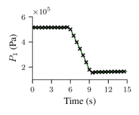
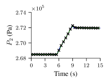
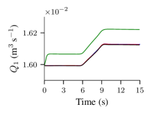
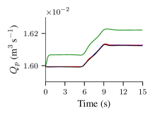
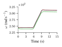
E.2 State estimation results for simulated data with noise

Table E.2: Mean absolute percentage error for the simulation with added noise case.

	$P_{1}$	$P_{2}$	$Q_{1}$	$Q_{2}$	$Q_{p}$	$\omega$
Case 1	0.2599347073369137	0.029908423147014734	0.009542642898642865	0.010517174084855772	0.010703753491727672	0.02554045837985367
Case 2	0.27755142957239837	0.026457354013453376	0.030153125673741597	0.027388373323869664	0.0304392975682618	1.6219662070529945
Case 3	0.5443767228377588	0.029139405665778436	0.0755574988515187	0.07811259323416116	0.07896161871581812	1.0122102158323114

(a) Intake pressure.

(b) Discharge pressure.

(c) Upstream volumetric flow rate.

(d) Downstream volumetric flow rate.

(e) Impeller volumetric flow rate.

(f) ESP angular velocity.

Fig. E.2: Predicted states for the simulated with noise and unknown flow parameters for the second investigation. Across all cases, the training dataset comprises $37$ data points and by $100$ collocation points.

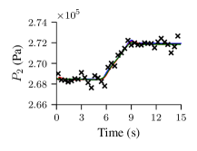
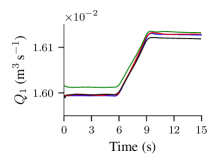
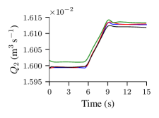
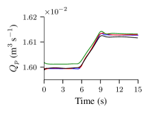
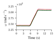
E.3 State estimation results for experimental data

Table E.3: Mean absolute percentage error for the experimental case.

	$P_{1}$	$P_{2}$	$Q_{1}$	$\omega$
Case 1	6.978218580436645	0.26434722951053674	0.09047458390235757	0.6626513291829126
Case 2	7.391333742267528	0.2532021274071301	0.33600542774150305	0.7506326322386131
Case 3	5.460018790378688	0.25160447841658956	0.1228899789251732	2.1666920722604632

(a) Intake pressure.

(b) Discharge pressure.

(c) Upstream flow rate.

(d) ESP angular velocity.

Fig. E.3: Predicted states for the experimental data and unknown flow parameters for the second investigation. Across all cases, the training dataset comprises $55$ data points and by $100$ collocation points.

References

- [1] André Paulo Ferreira Machado, Cassius Zanetti Resende and Daniel Cruz Cavalieri “Estimation and Prediction of Motor Load Torque Applied to Electrical Submersible Pumps” In Control Engineering Practice 84, 2019, pp. 284–296 DOI: 10.1016/j.conengprac.2018.11.019
- [2] Haiwen Zhu et al. “Performance Degradation and Wearing of Electrical Submersible Pump (ESP) with Gas-Liquid-Solid Flow: Experiments and Mechanistic Modeling” In Journal of Petroleum Science and Engineering 200, 2021, pp. 108399 DOI: 10.1016/j.petrol.2021.108399
- [3] Tan Nguyen “Artificial Lift Methods: Design, Practices, and Applications”, Petroleum Engineering Cham: Springer International Publishing, 2020 DOI: 10.1007/978-3-030-40720-9
- [4] M. A. Castillo et al. “Modal Parameters Estimation of an Electrical Submersible Pump Installed in a Test Well Using Numerical and Experimental Analysis” In Ocean Engineering 176, 2019, pp. 1–7 DOI: 10.1016/j.oceaneng.2019.02.035
- [5] P. Angeli and G. F. Hewitt “Pressure Gradient in Horizontal Liquid–Liquid Flows” In International Journal of Multiphase Flow 24.7, 1999, pp. 1183–1203 DOI: 10.1016/S0301-9322(98)00006-8
- [6] P. Angeli and G. F. Hewitt “Flow Structure in Horizontal Oil–Water Flow” In International Journal of Multiphase Flow 26.7, 2000, pp. 1117–1140 DOI: 10.1016/S0301-9322(99)00081-6
- [7] Wallace Honório, Daniel Lemos and Raone Lima “ESP Control and Monitoring System of Heavy Oil Peregrino Field” All Days, SPE Artificial Lift Conference - Latin America and Caribbean, 2015, pp. SPE–173929–MS DOI: 10.2118/173929-MS
- [8] Francesca Ravera et al. “Emulsification and emulsion stability: The role of the interfacial properties” In Advances in Colloid and Interface Science 288, 2021, pp. 102344 DOI: 10.1016/j.cis.2020.102344
- [9] Sunil Kokal “Crude-Oil Emulsions: A State-Of-The-Art Review” In SPE Production & Facilities 20.01, 2005, pp. 5–13 DOI: 10.2118/77497-PA
- [10] A. Perazzo, V. Preziosi and S. Guido “Phase Inversion Emulsification: Current Understanding and Applications” In Advances in Colloid and Interface Science 222, Reinhard Miller, Honorary Issue, 2015, pp. 581–599 DOI: 10.1016/j.cis.2015.01.001
- [11] Natan Augusto Vieira Bulgarelli et al. “A Novel Criterion Based on Slip Ratio to Assess the Flow Behavior of W/O Emulsions within Centrifugal Pumps” In Chemical Engineering Science 247, 2022, pp. 117050 DOI: 10.1016/j.ces.2021.117050
- [12] Natan Augusto Vieira Bulgarelli et al. “Relative Viscosity Model for Oil/Water Stable Emulsion Flow within Electrical Submersible Pumps” In Chemical Engineering Science 245, 2021, pp. 116827 DOI: 10.1016/j.ces.2021.116827
- [13] Jose Plasencia, Bjørnar Pettersen and Ole Jørgen Nydal “Pipe Flow of Water-in-Crude Oil Emulsions: Effective Viscosity, Inversion Point and Droplet Size Distribution” In Journal of Petroleum Science and Engineering 101, 2013, pp. 35–43 DOI: 10.1016/j.petrol.2012.11.009
- [14] Curtis R. Vogel “Computational Methods for Inverse Problems”, Frontiers in Applied Mathematics 23 Philadelphia: Society for Industrial and Applied Mathematics, 2002 DOI: 10.1137/1.9780898717570
- [15] Charles W. Groetsch “Inverse Problems in the Mathematical Sciences” Wiesbaden: Vieweg+Teubner Verlag, 1993 DOI: 10.1007/978-3-322-99202-4
- [16] Richard C Aster, Brian Borchers and Clifford H Thurber “Parameter Estimation and Inverse Problems” Waltham, MA: Academic Press, 2013 DOI: 10.1016/C2009-0-61134-X
- [17] Lennart Ljung and Torkel Glad “On Global Identifiability for Arbitrary Model Parametrizations” In Automatica 30.2, 1994, pp. 265–276 DOI: 10.1016/0005-1098(94)90029-9
- [18] R. Bellman and K. J. Åström “On Structural Identifiability” In Mathematical Biosciences 7.3, 1970, pp. 329–339 DOI: 10.1016/0025-5564(70)90132-X
- [19] Necibe Tuncer and Trang T. Le “Structural and Practical Identifiability Analysis of Outbreak Models” In Mathematical Biosciences 299, 2018, pp. 1–18 DOI: 10.1016/j.mbs.2018.02.004
- [20] Oana-Teodora Chis, Julio R. Banga and Eva Balsa-Canto “Structural Identifiability of Systems Biology Models: A Critical Comparison of Methods” In PLOS ONE 6.11 Public Library of Science, 2011, pp. e27755 DOI: 10.1371/journal.pone.0027755
- [21] Andreas Raue et al. “Comparison of Approaches for Parameter Identifiability Analysis of Biological Systems” In Bioinformatics 30.10, 2014, pp. 1440–1448 DOI: 10.1093/bioinformatics/btu006
- [22] Mario Castro and Rob J. Boer “Testing Structural Identifiability by a Simple Scaling Method” In PLOS Computational Biology 16.11 Public Library of Science, 2020, pp. e1008248 DOI: 10.1371/journal.pcbi.1008248
- [23] Ruiwen Dong, Christian Goodbrake, Heather A. Harrington and Gleb Pogudin “Differential Elimination for Dynamical Models via Projections with Applications to Structural Identifiability” In SIAM Journal on Applied Algebra and Geometry 7.1, 2023, pp. 194–235 DOI: 10.1137/22M1469067
- [24] Alejandro F. Villaverde and Gemma Massonis “On Testing Structural Identifiability by a Simple Scaling Method: Relying on Scaling Symmetries Can Be Misleading” In PLOS Computational Biology 17.10 Public Library of Science, 2021, pp. e1009032 DOI: 10.1371/journal.pcbi.1009032
- [25] J. O. Ramsay, G. Hooker, D. Campbell and J. Cao “Parameter Estimation for Differential Equations: A Generalized Smoothing Approach” In Journal of the Royal Statistical Society Series B: Statistical Methodology 69.5, 2007, pp. 741–796 DOI: 10.1111/j.1467-9868.2007.00610.x
- [26] Xin Qi and Hongyu Zhao “Asymptotic efficiency and finite-sample properties of the generalized profiling estimation of parameters in ordinary differential equations” In The Annals of Statistics 38.1 Institute of Mathematical Statistics, 2010, pp. 435 –481 DOI: 10.1214/09-AOS724
- [27] William Bradley and Fani Boukouvala “Two-Stage Approach to Parameter Estimation of Differential Equations Using Neural ODEs” In Industrial & Engineering Chemistry Research 60.45, 2021, pp. 16330–16344 DOI: 10.1021/acs.iecr.1c00552
- [28] Frank Dondelinger, Dirk Husmeier, Simon Rogers and Maurizio Filippone “ODE Parameter Inference Using Adaptive Gradient Matching with Gaussian Processes” In Proceedings of the Sixteenth International Conference on Artificial Intelligence and Statistics PMLR, 2013, pp. 216–228
- [29] H. Putter, S. H. Heisterkamp, J. M. A. Lange and F. de Wolf “A Bayesian Approach to Parameter Estimation in HIV Dynamical Models” In Statistics in Medicine 21.15, 2002, pp. 2199–2214 DOI: 10.1002/sim.1211
- [30] M. Raissi, P. Perdikaris and G. E. Karniadakis “Physics-Informed Neural Networks: A Deep Learning Framework for Solving Forward and Inverse Problems Involving Nonlinear Partial Differential Equations” In Journal of Computational Physics 378, 2019, pp. 686–707 DOI: 10.1016/j.jcp.2018.10.045
- [31] Atilim Gunes Baydin, Barak A. Pearlmutter, Alexey Andreyevich Radul and Jeffrey Mark Siskind “Automatic Differentiation in Machine Learning: a Survey” In Journal of Machine Learning Research 18.153, 2018, pp. 1–43 URL: http://jmlr.org/papers/v18/17-468.html
- [32] Ameya D. Jagtap, Ehsan Kharazmi and George Em Karniadakis “Conservative physics-informed neural networks on discrete domains for conservation laws: Applications to forward and inverse problems” In Computer Methods in Applied Mechanics and Engineering 365, 2020, pp. 113028 DOI: 10.1016/j.cma.2020.113028
- [33] Ameya D. Jagtap and George Em Karniadakis “Extended Physics-Informed Neural Networks (XPINNs): A Generalized Space-Time Domain Decomposition Based Deep Learning Framework for Nonlinear Partial Differential Equations” In Communications in Computational Physics 28.5, 2020, pp. 2002–2041 DOI: 10.4208/cicp.OA-2020-0164
- [34] Ehsan Kharazmi, Zhongqiang Zhang and George E.M. Karniadakis “hp-VPINNs Variational physics-informed neural networks with domain decomposition” In Computer Methods in Applied Mechanics and Engineering 374, 2021, pp. 113547 DOI: 10.1016/j.cma.2020.113547
- [35] Xuhui Meng, Zhen Li, Dongkun Zhang and George Em Karniadakis “PPINN: Parareal physics-informed neural network for time-dependent PDEs” In Computer Methods in Applied Mechanics and Engineering 370, 2020, pp. 113250 DOI: 10.1016/j.cma.2020.113250
- [36] Junwoo Cho et al. “Separable PINN: Mitigating the Curse of Dimensionality in Physics-Informed Neural Networks”, 2022 arXiv:2211.08761 [cs.LG]
- [37] Levi McClenny and Ulisses Braga-Neto “Self-Adaptive Physics-Informed Neural Networks using a Soft Attention Mechanism”, 2022 arXiv:2009.04544 [cs.LG]
- [38] Sigurdur Mar Valsson Ivan Depina and Hrvoje Gotovac “Application of physics-informed neural networks to inverse problems in unsaturated groundwater flow” In Georisk: Assessment and Management of Risk for Engineered Systems and Geohazards 16.1 Taylor & Francis, 2022, pp. 21–36 DOI: 10.1080/17499518.2021.1971251
- [39] Kamaljyoti Nath, Xuhui Meng, Daniel J. Smith and George Em Karniadakis “Physics-informed neural networks for predicting gas flow dynamics and unknown parameters in diesel engines” In Scientific Reports 13, 2023, pp. 13683 DOI: 10.1038/s41598-023-39989-4
- [40] Ameya D. Jagtap, Zhiping Mao, Nikolaus Adams and George Em Karniadakis “Physics-informed neural networks for inverse problems in supersonic flows” In Journal of Computational Physics 466, 2022, pp. 111402 DOI: 10.1016/j.jcp.2022.111402
- [41] Maurício de Melo Freire Figueiredo, Felipe C. T. Carvalho, Ana Maria Frattini Fileti and Alberto Luiz Serpa “Flow pattern classification in water-air vertical flows using a single ultrasonic transducer” In Experimental Thermal and Fluid Science 119, 2020, pp. 110189 DOI: j.expthermflusci.2020.110189
- [42] K. Tanaka et al. “Detailed Bond Graph Models of Turbomachinery” In 2000 26th Annual Conference of the IEEE Industrial Electronics Society. IECON 2000. 2000 IEEE International Conference on Industrial Electronics, Control and Instrumentation. 21st Century Technologies 3, 2000, pp. 1550–1555 vol.3 DOI: 10.1109/IECON.2000.972505
- [43] H. Higo et al. “Bondgraph Analysis on Pressure Fluctuation in Hydraulic Pipes” In 2000 26th Annual Conference of the IEEE Industrial Electronics Society. IECON 2000. 2000 IEEE International Conference on Industrial Electronics, Control and Instrumentation. 21st Century Technologies and Industrial Opportunities (Cat. No.00CH37141) 3 Nagoya, Japan: IEEE, 2000, pp. 1556–1561 DOI: 10.1109/IECON.2000.972506
- [44] H. C. Brinkman “The Viscosity of Concentrated Suspensions and Solutions” In The Journal of Chemical Physics 20.4, 2004, pp. 571–571 DOI: 10.1063/1.1700493
- [45] A. Einstein “Eine neue Bestimmung der Moleküldimensionen” Cited by: 2708; All Open Access, Green Open Access In Annalen der Physik 324.2, 1906, pp. 289 – 306 DOI: 10.1002/andp.19063240204
- [46] Geoffrey Ingram Taylor “The viscosity of a fluid containing small drops of another fluid” In Proc. R. Soc. Lond. A Math. Phys. Sci. 138.834, 1932, pp. 41–48 DOI: 10.1098/rspa.1932.0169
- [47] Rajinder Pal and Edward Rhodes “Viscosity/Concentration Relationships for Emulsions” In Journal of Rheology 33.7, 1989, pp. 1021–1045 DOI: 10.1122/1.550044
- [48] Christopher Rackauckas and Qing Nie “DifferentialEquations.jl – A Performant and Feature-Rich Ecosystem for Solving Differential Equations in Julia” In Journal of Open Research Software, 2017 DOI: 10.5334/jors.151
- [49] Mitchell Daneker, Zhen Zhang, George Em Karniadakis and Lu Lu “Systems Biology: Identifiability Analysis and Parameter Identification via Systems-Biology-Informed Neural Networks” In Computational Modeling of Signaling Networks New York, NY: Springer US, 2023, pp. 87–105 DOI: 10.1007/978-1-0716-3008-2_4
- [50] Hongyu Miao, Xiaohua Xia, Alan S. Perelson and Hulin Wu “On Identifiability of Nonlinear ODE Models and Applications in Viral Dynamics” In SIAM Review 53.1, 2011, pp. 3–39 DOI: 10.1137/090757009