\WithSuffix
[1];
// #1
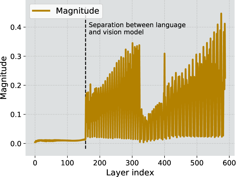 (a) Weight Magnitudes
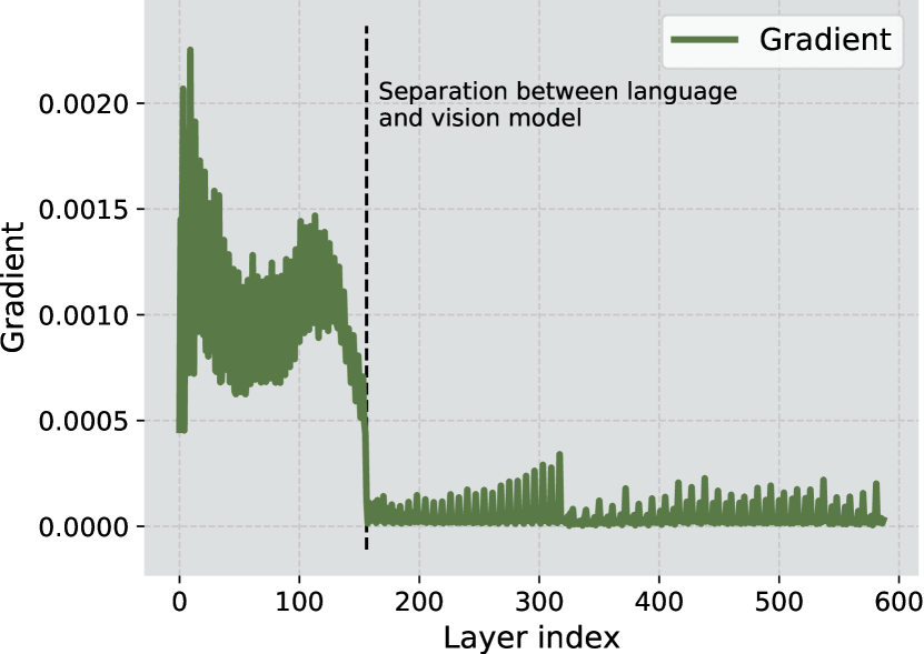 (b) Weight Gradients
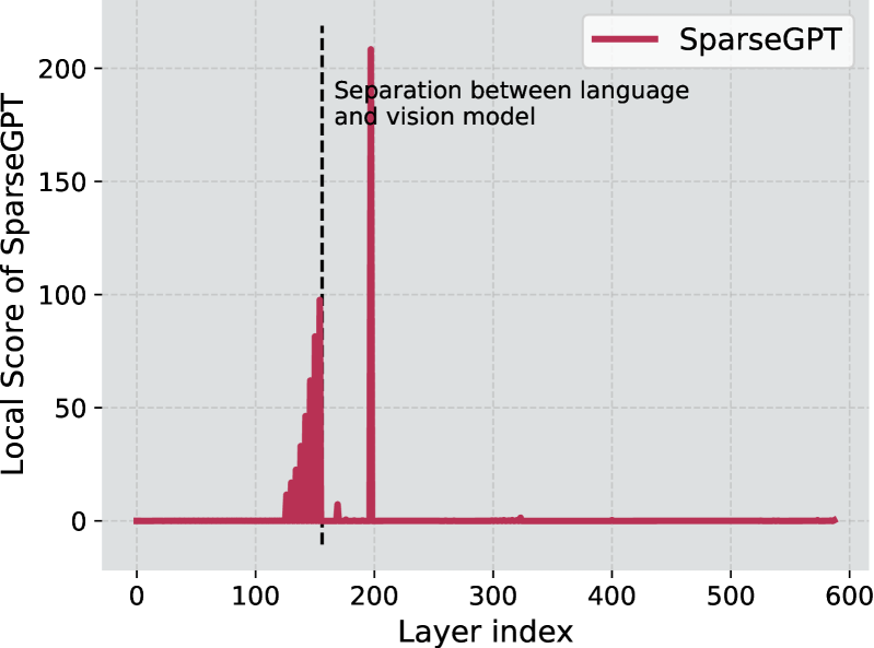 (c) Local Score of SparseGPT
Figure 1: (a) and (b): The imbalance of the magnitude and gradient distributions between vision and language models. (c): The skewed distribution of the layer-wise scores of SparseGPT.
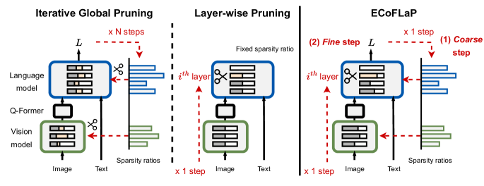 Figure 2: Illustration of our ECoFLaP compared to global and layer-wise pruning. The boxes with a
blue, green, and black
border denote the language, vision, and Q-Former modules, respectively. The dotted red arrows show the working flow of the algorithm. The beige color indicates the pruning of the current step (layer) is conditioned on the pruning decisions made in the preceding steps (layers), which are marked in gray. ECoFLaP first performs the efficient coarse step to obtain the pruning ratio for each layer by leveraging the zeroth-order gradient, and then removes the uncritical weights in a layer-wise fashion in the fine step.
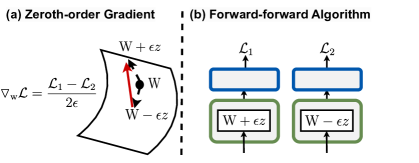 Figure 3: Illustration of (a) the zeroth-order gradient in weight space, and (b) the forward-forward algorithm.
In the previous section, we introduce our coarse-to-fine pruning framework to determine the pruning ratios for layer-wise pruning. Note that our goal is to prune models with billions of parameters, so we again focus on the one-shot setting in this step without any iterative refinement. To this end, our first attempt is to use the first-order backward gradient with weight magnitude (LeCun et al., 1989), , as the global importance score, and the performance improvement demonstrates the effectiveness of our framework (Please see Table 1 and Figure 4). However, even though the first-order backward gradient is still tractable for most models. like less than 5B parameters, 7B LLaMA (Touvron et al., 2023) requires more than 40GB even with float16 weight type and batch size being one.
To further reduce the cost of computing gradients, we instead compute the zeroth-order approximated gradient by replacing the backpropagation with the forward-forward algorithm (Hinton, 2022; Malladi et al., 2023).
We take the layer of a model as an example, the zeroth-order gradient of can be computed by perturbing the weight with Gaussian noises twice, that is,
(5)
We hence use as the importance score of . Note that we do not multiply it with the weight magnitude as solely using the approximated gradients works better empirically. The computation of Equation 5 is extremely memory-efficient and the exact process for the layer is shown in the following: (1) First, we choose a random seed and then sample a noise (now we use 2x of memory of “this layer”), (2) we modify the model’s weight with and compute the loss change , (3) we then sample the same noise as the first step (by setting the same random seed), and we modify the model’s weight with , which can be done by subtracting from the previous weight, and compute , (4) obtain the gradient norm by ( (all terms are scalars). From the above process, for an N-layer network, we only need (N+1) times of one-layer memory, which is significantly memory-efficient than storing the whole gradients that cause 2N times of one-layer memory. This explains why our approach uses much less memory than first-order based methods, which also need to cache input activations. One may suspect we need to sample many noises to capture the loss of the landscape and to estimate the gradient accurately. However, our experiments and the previous studies (Malladi et al., 2023) show that one noise is sufficient. We describe our approach in detail in Algorithm 1.
 (a) BLIP-2 on VQA
 (b) FlanT5 on MMLU
 (c) EVA-ViT on ImageNet
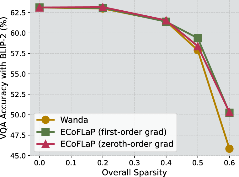
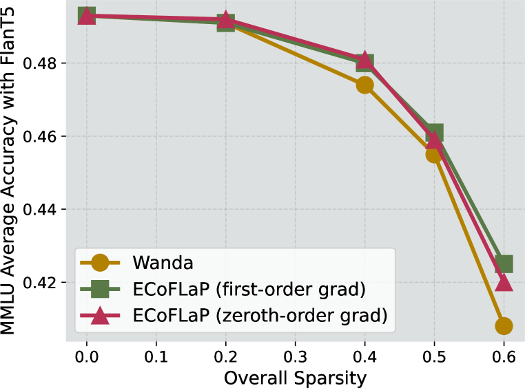
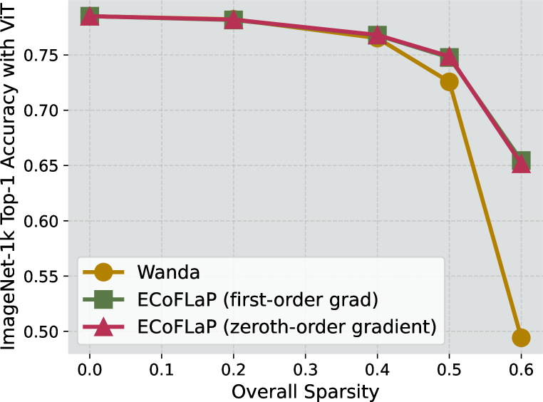
Figure 4: The accuracy and model sparsity trade-off for Wanda, ECoFLaP with first-order and zeroth-order gradient on both BLIP-2 (multimodal), FlanT5 (unimodal), and EVA-ViT (unimodal).
Visualization and Analysis. We also provide the visualization of the sparsity ratios obtained by ECoFLaP (Figure 6) and the loss landscape of BLIP-2 (Section 8) to justify the use of zeroth-order optimization. In Figure 6, we observe that our ECoFLaP variants allocate sparsity ratios in a similar distribution, in favor of lower sparsity ratios for the visual model and higher sparsity ratios for the language model, and this alignment provides evidence that the zeroth-order gradient obtained by the forward-forward algorithm can be the accurate but cheaper alternative to the first-order gradient in importance estimation. The landscape shown in Section 8 presents that BLIP-2 is located at a smooth basin with a single local minimum. This loss landscape justifies the success of utilizing zeroth-order optimization as we avoid sampling weights located in other basins that may cause an inaccurate gradient estimation. We also present a qualitative analysis of the pruned model in Appendix E.
Input: weights of the vision model , weights of the language model , calibration dataset , target sparsity , maximum sparsity per layer
Output: The pruned weights and
1
// Coarse step: determine the sparsity ratios via global information
2
// *
3get the global importance score
// *
4obtain the sparsity via Equation 3
// Fine step: perform layer-wise pruning
5
6
// We initialize the weight to be the identity matrix, depicting the fact that the input of the first layer is the raw input.
7
8
9for = to do
// *
10 prune vision weights layer by layer
11
12
13
14for = to do
// *
15 prune language weights layer by layer
16
17
18return
Algorithm 1 Efficient Coarse-to-Fine Layer-wise Pruning
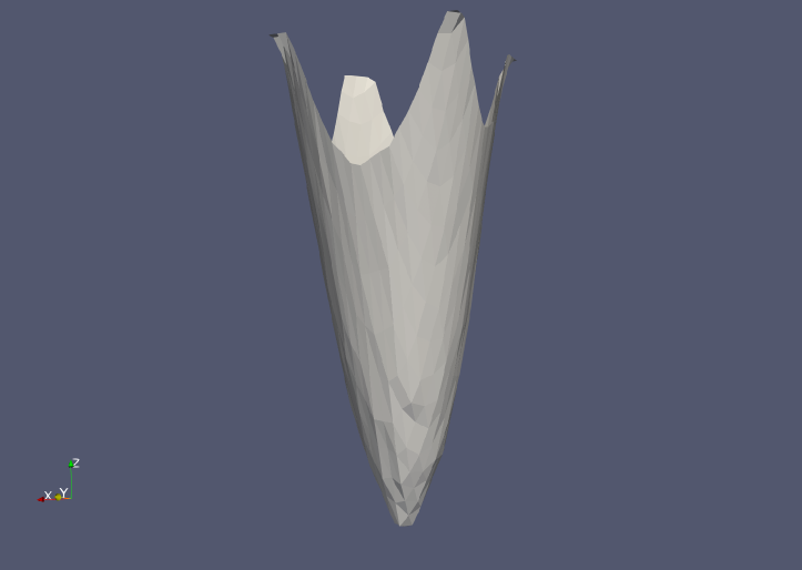 Figure 5: The loss landscape of the BLIP-2 model.
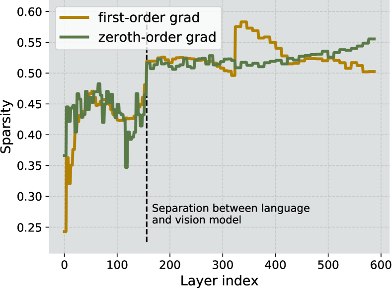
Figure 6: Sparsity ratios obtained by ECoFLaP.
![[Uncaptioned image]](/html/2310.02998/assets/figures/microwave_example.jpg)
![[Uncaptioned image]](/html/2310.02998/assets/figures/car_example.jpg)
![[Uncaptioned image]](/html/2310.02998/assets/figures/horse_example.jpg) Question ID
202174017
20984557
20602949
Questions
What shape is the microwave the stove is below?
Which kind of vehicle is parked on the street?
What is the horse running across?
Ground Truth
rectangular
car
ground
Full Model’s
Prediction
square
car
hill
ECoFLaP-pruned
Model’s Prediction
rectangular
bicycle
rocks
Question ID
202174017
20984557
20602949
Questions
What shape is the microwave the stove is below?
Which kind of vehicle is parked on the street?
What is the horse running across?
Ground Truth
rectangular
car
ground
Full Model’s
Prediction
square
car
hill
ECoFLaP-pruned
Model’s Prediction
rectangular
bicycle
rocks
ECoFLaP: Efficient Coarse-to-Fine Layer-Wise Pruning for Vision-Language Models
Abstract
Large Vision-Language Models (LVLMs) can understand the world comprehensively by integrating rich information from different modalities, achieving remarkable advancements on various multimodal downstream tasks. However, deploying LVLMs is often problematic due to their massive computational/energy costs and carbon consumption. Such issues make it infeasible to adopt conventional iterative global pruning, which is costly due to computing the Hessian matrix of the entire large model for sparsification. Alternatively, several studies have recently proposed layer-wise pruning approaches to avoid the expensive computation of global pruning and efficiently compress model weights according to their importance within a layer. However, they often suffer from suboptimal model compression due to their lack of a global perspective. To address this limitation in recent efficient pruning methods for large models, we propose Efficient Coarse-to-Fine Layer-Wise Pruning (ECoFLaP), a two-stage coarse-to-fine weight pruning approach for LVLMs. We first determine the sparsity ratios of different layers or blocks by leveraging the global importance score, which is efficiently computed based on the zeroth-order approximation of the global model gradients. Then, the model performs local layer-wise unstructured weight pruning based on globally-informed sparsity ratios. We validate our proposed method across various multimodal and unimodal models and datasets, demonstrating significant performance improvements over prevalent pruning techniques in the high-sparsity regime. ††Our project page and code are available at https://ecoflap.github.io/1 Introduction
Deep learning models have been increasingly growing in size (Radford et al., 2018; Brown et al., 2020; Liu et al., 2023; Zhu et al., 2023) in order to have a sufficient capacity to learn challenging tasks in the real world. However, this exorbitant model size requires significant computations and memory to deploy, which limits their applicability in many resource-constrained environments. Model compression, a strategy to reduce the size of neural networks while preserving their capabilities (Dai et al., 2018; Park et al., 2022; Xiao et al., 2023; Fang et al., 2023), has gained popularity in tackling this problem. In order to build lighter, faster, and more interpretable models, various directions have been studied in parallel, including model pruning (Dai et al., 2018; Fang et al., 2023; Frantar & Alistarh, 2023), quantization (Park et al., 2022; Xiao et al., 2023), layer drop (Sajjad et al., 2023), and token merging (Bolya et al., 2022; Bolya & Hoffman, 2023). Among them, in this paper, we study an unstructured model pruning approach that has strong potential to preserve model performance, even with a high compression rate of large vision-language models. While most model pruning approaches tackle the problem of vision-based tasks (Liang et al., 2022b; Kong et al., 2022; Wei et al., 2023) and a few recent works have studied to reduce the size of language models (Ma et al., 2023; Sun et al., 2023a; Frantar & Alistarh, 2023), efficient pruning for multimodal models like Large Vision-Language Models (LVLMs) (Ye et al., 2023; Li et al., 2023a) have been understudied due to their architectural complexity and the disparities in data characteristics between different modalities (Shi et al., 2023). Unlike unimodal learning methods, network architectures for multimodal learning (Li et al., 2022; 2023c) are often composed of modality-specific sub-modules to capture the knowledge for each modality, which substantially expands the scale of multimodal models. Moreover, this modularization leads to significant imbalances in the weight/gradient distributions between modules associated with different modalities, making unified pruning difficult. As conventional iterative pruning (Mallya & Lazebnik, 2018; Molchanov et al., 2019; Wang et al., 2020; Zhang et al., 2022b) demands extensive computations to learn pruning masks by computing the inverse Hessian in large models, layer-wise one-shot pruning (Chen & Zhao, 2018; Frantar & Alistarh, 2023; Sun et al., 2023a) has recently been developed to compress them efficiently. These approaches discard uninformative model weights in a single iteration without computing the expensive second-order Hessian matrix for the entire model architecture, yet often suffer from finding the optimal sparsity ratio per layer, as they resort to intra-layer weight importance without sufficient understanding of global (i.e., inter-layer) weight correlations in the model, hence leading to suboptimal pruning. To overcome this limitation of layer-wise pruning and build an efficient approach for LVLM compression, we propose Efficient Coarse-to-Fine Layer-Wise Pruning (ECoFLaP) that obtains an adaptive sparsity ratio per layer in a single step based on a ‘global importance score’ (Coarse) and then removes parameters that are less critical (to the model’s performance), in a layer-wise manner (Fine). Note that our proposed method is computationally efficient by leveraging the first-order gradient to obtain a global importance score without Hessian operations, allowing layer-wise pruning to leverage a holistic correlation across the model weights. To further improve the memory efficiency of the global score computation, we introduce the zeroth-order approximate gradient computed by the forward-forward algorithm (Malladi et al., 2023; Hinton, 2022). In the end, our ECoFLaP obtains highly compressed large models in a single shot, with adaptive sparsity in each layer, leveraging global weight importance approximated by memory-efficient forward-forward operations. We note that our proposed pruning method generalizes well not only to vision-language multimodal tasks but also to unimodal tasks, including ImageNet (Vision) and MMLU (NLP). We extensively validate the efficacy of our approach across a variety of models and datasets, including but not limited to EVA-ViT, FlanT5, LLaMA, BLIP/BLIP-2, CLIP, and on image classification (ImageNet-1k), multitask multiple-choice question answering (MMLU), next token prediction (WikiText), visual reasoning (NLVR2), visual question answering (VQAv2, OK-VQA, GQA), image captioning (NoCaps, COCO Captions), and image-text retrieval (Flickr30k). Our proposed ECoFLaP surpasses iterative global pruning and SoTA layer-wise pruning methods, SparseGPT (Frantar & Alistarh, 2023) and Wanda (Sun et al., 2023a), with relative improvements up to in average performance across multiple VL tasks. Additionally, our approach outperforms a recent SoTA in pruning vision-language model, UPop (Shi et al., 2023), achieving relative improvements of 1.8% and 2.6% on NLVR2 and COCO captions. ECoFLaP also generalizes well to unimodal models (FlanT5, LLaMA, EVA-ViT), particularly in a higher sparsity regime. It is worth noting that ECoFLaP with the zeroth-order gradient reduces the GPU memory usage by up to compared to baselines using the first-order gradient to estimate the global importance. These results not only underscore the potential of our method but also pave the way for more efficient and effective pruning techniques in the future. We summarize our contributions as threefold: • We propose a novel layer-wise pruning method for vision-language models, coined Efficient Coarse-to-Fine Layer-Wise Pruning for Vision-Language Models (ECoFLaP), that finds adaptive sparsity per layer by leveraging the global importance score approximated via zeroth-order gradients. • We validate the proposed method on various backbone structures with diverse vision-language and unimodal tasks, and demonstrate the superiority of our method by consistently outperforming the SoTA pruning baselines for large models on multiple benchmark datasets. • We provide extensive analyses and ablation studies that help to understand the challenges of unified multimodal model pruning and the strengths of our proposed methods compared to baselines, including visualizations of importance score distribution, dynamic sparsity, loss landscape, etc.2 Related Work
Model pruning for transformers.
Efficient model inference via pruning (Yoon & Hwang, 2017; Dai et al., 2018; Zhang et al., 2022a; Fang et al., 2023) is one of the long-standing topics in the community and is coming to the fore as transformer-based models grow in size. Model pruning is typically categorized into structured pruning and unstructured pruning. The former (McCarley et al., 2019; Wang et al., 2019; Kwon et al., 2022) aims to accelerate inference speed and throughput at the expense of model performance. Unstructured pruning (Sun et al., 2023a; Frantar & Alistarh, 2023), on the other hand, can be advantageous in preserving performance even with high model sparsity given AI acceleration software or sparse matrix computation schemes (Han et al., 2016; Mishra et al., 2021; Das & Ramamoorthy, 2022; NeuralMagic, 2022). Recently, Frantar & Alistarh (2023) suggest a one-shot pruning technique, SparseGPT, for generated pre-trained transformers (GPTs) in an unstructured manner. They newly employ a sparse regression solver that prunes weights at each layer based on row-wise Hessian reconstruction as formulated by a closed-form solution. Wanda (Sun et al., 2023a) proposes a magnitude-based unstructured pruning approach for large language models (LLMs). It promotes layer-wise weight sparsification based on the importance, computed by multiplying weights and input activations. However, these SoTA pruning methods rely on the pre-defined pruning ratio that all layers resort to the same sparsity, restricting the upper bound on model compression. In addition, their methods are tailored to language models without concern for different modalities. On the other hand, our proposed method allows adaptive pruning at each layer without heavy computation of global gradients. Further, to the best of our knowledge, we propose a first unified sparse approximate solver for vision-language multimodal models.Transformers for vision-language multimodal learning.
Vision-language multimodal learning has shown remarkable achievement on various tasks, such as classification (Liu et al., 2018; Liang et al., 2022a), retrieval (Fei et al., 2021), few-shot learning (Tsimpoukelli et al., 2021; Alayrac et al., 2022), visual QA (Kim et al., 2016; Liu et al., 2023), and image/video generation (Zhou et al., 2022b; Singer et al., 2022; Lee et al., 2023). Recently, transformer modules have become the new standard for both language and visual-based (Dosovitskiy et al., 2020; Liu et al., 2021) tasks, and the powerful representation of these transformers allows for the modularization of multimodal learning frameworks with existing pre-trained uni-modal models without an expensive re-training phase for multimodal data (Radford et al., 2021; Zhou et al., 2022a).3 Background: Layer-wise Pruning for Vision-language Models
3.1 Preliminaries: A Framework for Vision-language Models
Multiple vision-language multimodal models introduce different architectural designs to understand compositional multimodal semantics, which can affect the pruning strategy. In this paper, we basically build our pruning method upon two popular multimodal learning frameworks for vision-language tasks, BLIP (Li et al., 2022) and BLIP-2 (Li et al., 2023c), which are modularized with the pre-trained ViT (Dosovitskiy et al., 2020) and FlanT5 (Chung et al., 2022) architectures to encode visual and language information, respectively. They have achieved remarkable zero-shot performance on various vision-language tasks. Let the visual encoder and language model in BLIP variants be composed of a set of the weights and , respectively, where and indicate the number of the corresponding layers. While freezing these pre-trained backbones, BLIPs introduce Query transformer (Q-Former) , a lightweight module with a set of the weights , that extracts essential information from visual representation and warps it to the input space of the language model (Li et al., 2021). Given the multimodal input pair , the output of the model is represented as , where denotes the aligned visual representation .3.2 Challenges in Pruning Vision-language Models
Let us first describe a primary strategy for Hessian-based global pruning, which aims to remove the optimal subset111The subset size (i.e., sparsity) is often pre-defined or obtained through training. of parameters minimizing the loss change . Here, w denotes the weight vector of the model. When the model parameter is removed, implying , where indicates the canonical basis vector, its importance is represented as . After that, the model prunes its weights with the lowest importance. However, computing the inverse Hessian requires significant computational budgets and is often infeasible for large models. On the other hand, layer-wise one-shot pruning aims to leverage a small amount of calibration data (such as 128 data points) to remove less important weights from the model in a single step based on their local significance per layer. This approach is significantly efficient in terms of computation/memory in the model pruning phase without expensive iterations of the re-training or Hessian matrix computation for the parameters of the entire model, which is particularly beneficial for large language/multimodal models with billions of parameters. The model compression procedure of recent layer-wise pruning methods (Lazarevich et al., 2021; Yu & Xiang, 2023; Frantar & Alistarh, 2023) can be summarized in the three steps given a target sparsity of and a layer index : (1) Compute the importance score for each parameter within the layer , (2) Discard of the parameters of layer based on their importance score and adjust the remaining weights (usually for Hessian-based methods), and (3) calculate the layer’s output with only activated (i.e., not pruned) weights, and repeat the process for the next layer () until . However, most layer-wise pruning approaches focus on removing unnecessary weights or parameters from single-modal models, such as vision-only (Chen & Zhao, 2018; Lazarevich et al., 2021; Yu & Xiang, 2023) or language-only (Frantar & Alistarh, 2023; Sun et al., 2023a) architectures, which face significant limitations when extended to multimodal (e.g., vision-language) models due to the critical gap in weight/gradient distributions between different modalities, as shown in Figures 1(a) and 1(b). Unlike global pruning methods estimating the importance of each parameter based on the objective loss, layer-wise pruning without the guidance of global weight correlations suffers from obtaining relative significance across weights in different layers/modules due to such severe distributional imbalances in the different modality modules. For example, in Wanda, inputs for different layers significantly vary in their scales (Ba et al., 2016; Ioffe & Szegedy, 2015), and in SparseGPT, the importance of the local loss functions for different layers is also incomparable (Please see the skewed distribution of the local score shown in Figure 1(c)). This problem makes layer-wise pruning approaches usually set the pruning ratio to be a fixed value for all layers, resulting in a suboptimal compression rate and performance. This is also evident in the results from Singh & Alistarh (2020) that the global WoodFisher pruner outperforms its layer-wise counterpart by a large margin, especially at high sparsity regimes. (a) Weight Magnitudes
 (b) Weight Gradients
 (c) Local Score of SparseGPT
4 ECoFLaP: Efficient Coarse-to-Fine Layer-Wise Pruning
As discussed above, deploying a layer-wise pruning approach for large vision-language models is challenging due to three primary issues; distributional/architectural disparity between different modalities, significantly large model size, and lack of global knowledge. To overcome such critical challenges, we propose Efficient Coarse-to-Fine Layer-wise Pruning (ECoFLaP), to efficiently compute an adaptive pruning ratio for each layer with global importance scores (Coarse), and then accurately remove the parameters layer by layer with local significance (Fine). Figure 2: Illustration of our ECoFLaP compared to global and layer-wise pruning. The boxes with a
blue, green, and black
border denote the language, vision, and Q-Former modules, respectively. The dotted red arrows show the working flow of the algorithm. The beige color indicates the pruning of the current step (layer) is conditioned on the pruning decisions made in the preceding steps (layers), which are marked in gray. ECoFLaP first performs the efficient coarse step to obtain the pruning ratio for each layer by leveraging the zeroth-order gradient, and then removes the uncritical weights in a layer-wise fashion in the fine step.
4.1 The framework of coarse-to-fine layer-wise pruning
Our focus is to prune the BLIP-like multimodal architectures, as discussed in Section 3.1. Note that we compress the vision and language model in BLIP variants while keeping Q-Former intact because it is sufficiently lightweight, occupying only of the parameters in the whole framework. Given the multimodal calibration data , a conventional layer-wise pruning method aims to find the sparse weight at layer via the corresponding local objective : (1) where is the score function to compute the importance of the weight, is denoted as the pruned weight from , and the desired sparsity at layer . Basically, is the same for all layers in layer-wise pruning methods. In our proposed Efficient Coarse-to-Fine Layer-wise Pruning (ECoFLaP) framework, we estimate the optimal sparsity for each layer in the vision-language model by computing the global importance of model weights. One straightforward direction to obtain the layer sparsities is to perform global pruning on the model for the target global sparsity by leveraging the global loss objective , (2) Then, we can estimate the layer sparsity via . However, this approach requires an expensive operation to obtain gradients for all weights in the large model and to extract the pruned weights via argmax, consuming enormous memory and computational resources. Therefore, we introduce an alternative numerical approach, which computes the keep ratio (1 - sparsity ratio) based on importance scores linearly, to avoid expensive operations that can estimate the global importance score efficiently. First, we obtain the importance score for each weight via the global objective function, namely, , and then convert the scores to sparsity by three steps: (1) Find the total parameters that need to be selected based on , (2) Normalize the scores, (3) Obtain the sparsity for each layer based on the number of parameters to be picked and the parameters of this layer. The example to determine the sparsity ratio for the layer of the model is shown below, (3) (4) We then inject the derived sparsity ratios back to Equation 1 to prune the model layer-wisely. We also introduce a hyperparameter to control the maximum sparsity for each layer to avoid the layer collapse, which is discovered by previous literature (Tanaka et al., 2020) that the global pruning approach may remove all the parameters for one layer. To incorporate this hyperparameter in the Equation 3, we simply pre-pick the parameters for each layer to satisfy the max sparsity condition, subtracting the with the number of pre-picked parameters, and start the algorithm. In our experiments, we find using the same sparsity ratio for the layers in one block (such as the feed-forward layer and attention layer in a transformer block) makes the results more robust, so we also extend the algorithm to determine group sparsity ratios by via group scores (aggregating all the layer scores in a block). For the layer-wise pruning step, we utilize Wanda, which combines the input activation of the layer with the weight magnitude as the local importance score, to remove uncritical parameters based on the obtained layer sparsity ratios.4.2 Zeroth-order global information
 Figure 3: Illustration of (a) the zeroth-order gradient in weight space, and (b) the forward-forward algorithm.
In the previous section, we introduce our coarse-to-fine pruning framework to determine the pruning ratios for layer-wise pruning. Note that our goal is to prune models with billions of parameters, so we again focus on the one-shot setting in this step without any iterative refinement. To this end, our first attempt is to use the first-order backward gradient with weight magnitude (LeCun et al., 1989), , as the global importance score, and the performance improvement demonstrates the effectiveness of our framework (Please see Table 1 and Figure 4). However, even though the first-order backward gradient is still tractable for most models. like less than 5B parameters, 7B LLaMA (Touvron et al., 2023) requires more than 40GB even with float16 weight type and batch size being one.
To further reduce the cost of computing gradients, we instead compute the zeroth-order approximated gradient by replacing the backpropagation with the forward-forward algorithm (Hinton, 2022; Malladi et al., 2023).
We take the layer of a model as an example, the zeroth-order gradient of can be computed by perturbing the weight with Gaussian noises twice, that is,
(5)
We hence use as the importance score of . Note that we do not multiply it with the weight magnitude as solely using the approximated gradients works better empirically. The computation of Equation 5 is extremely memory-efficient and the exact process for the layer is shown in the following: (1) First, we choose a random seed and then sample a noise (now we use 2x of memory of “this layer”), (2) we modify the model’s weight with and compute the loss change , (3) we then sample the same noise as the first step (by setting the same random seed), and we modify the model’s weight with , which can be done by subtracting from the previous weight, and compute , (4) obtain the gradient norm by ( (all terms are scalars). From the above process, for an N-layer network, we only need (N+1) times of one-layer memory, which is significantly memory-efficient than storing the whole gradients that cause 2N times of one-layer memory. This explains why our approach uses much less memory than first-order based methods, which also need to cache input activations. One may suspect we need to sample many noises to capture the loss of the landscape and to estimate the gradient accurately. However, our experiments and the previous studies (Malladi et al., 2023) show that one noise is sufficient. We describe our approach in detail in Algorithm 1.
5 Experimental Setup
We report evaluation metrics and more experimental details in Appendix C. Architectures. We use multiple uni- and multi-modal architectures for experiments: the encoder-decoder vision of BLIP-2 (Li et al., 2023c), composed of pre-trained EVA-ViT (ViT-g/14 from EVA-CLIP) (Sun et al., 2023b) and FlanT5 (Chung et al., 2022), is used for most experiments and ablation studies. And, we also extend our approach to BLIP (Li et al., 2022) with ViT (Dosovitskiy et al., 2020) and BERT (Devlin et al., 2019) backbones. In addition, we evaluate our approach solely on unimodal vision and NLP tasks with EVA-ViT, FlanT5, and LLaMA backbones. Evaluation Datasets. We evaluate the zero-shot ability of BLIP-2 on various datasets after pruning, such as VQAv2, OK-VQA, and GQA for visual question answering, NoCaps for image captioning, and Flickr30k for image-text retrieval. For BLIP, we evaluate the performance change of the BLIP fine-tuned on NLVR2 and COCO captions. For unimodal models, we evaluate FlanT5 on MMLU, evaluate LLaMA 7B with WikiText, and evaluate EVA-ViT with ImageNet-1k. Baselines. We compare ECoFLaP to several global pruning and layer-wise pruning approaches. For Global Magnitude Pruning, we perform global pruning based on the magnitude of the weight. Gradient-based Pruning is an iterative global pruning approach, where we use the multiplication of the first-order gradient and the weight magnitude as the importance score and prune the model to target sparsity in 3 iterations. SparseGPT is a layer-wise Hessian-based method. Wanda is also a layer-wise approach utilizing the multiplication of the weight magnitude and the norm of input activation as the local importance score. The comparison of the above pruning methods and their importance metric can be found in Table 8. We also compare our method with UPop, which prunes and re-trains the vision-language model simultaneously in a unified progressive pruning manner.6 Results
Table 1: Comparison of existing pruning approaches with ECoFLaP on the zero-shot performance with BLIP-2 at 0.5 sparsity. We report accuracy for visual question answering, CIDEr and SPICE for image captioning, and TR@1 (text recall) and IR@1 (image recall) for image retrieval. We also compute the macro average score over tasks and the GPU memory usage for each method. Method Sparsity Method’s Mem. Usage (GB) Visual Question Answering Image Captioning Image retrieval Macro Avg. VQAv2 OK-VQA GQA NoCaps Flickr30k Accuracy CIDEr SPICE TR@1 IR@1 Full Model 0% - 63.1 41.1 44.1 121.7 15.8 97.6 89.7 62.1 Global Magnitude Pruning 50% 8.46 0.0 0.0 0.0 0.0 0.0 0.2 0.1 0.0 Gradient-based Pruning 50% 22.4 56.9 35.3 41.7 96.8 13.5 93.0 82.4 55.4 SparseGPT 50% 9.04 57.4 36.1 40.8 108.1 14.1 96.4 86.3 57.4 Wanda 50% 8.87 57.9 35.3 42.2 106.9 14.1 95.1 84.6 57.2 ECoFLaP + First-order Gradient 50% 22.4 59.4 36.3 42.3 109.9 14.2 95.9 86.2 58.2 + Zeroth-order Gradient 50% 8.93 58.4 35.6 42.9 110.2 14.3 95.5 85.8 58.0 (a) BLIP-2 on VQA
 (b) FlanT5 on MMLU
 (c) EVA-ViT on ImageNet
6.1 Main experimental results
We demonstrate the zero-shot performance on various datasets using BLIP-2 pruned by our ECoFLaP and baselines at a 0.5 sparsity ratio in Table 1. And we compare our approach with UPop using BLIP backbone on NLVR2 and COCO captions under the fine-tuning and non-fine-tuning settings in Table 3. We also provide the comparison of our approach and Wanda at various sparsities on both multi- and uni-modal models in Figure 4. We summarize our observations as follows: ECoFLaP consistently outperforms Global Magnitude Pruning (GMP) and Gradient-based Pruning as shown in Table 1. GMP fails to generate meaningful results at 0.5 sparsity. In particular, we find that GMP suffers from pruning the vision module, EVA-ViT, so the degraded visual representation harms the multimodal model performance. Gradient-based Pruning performs significantly better by selecting crucial weights based on gradient information of the whole model, but it requires a larger memory than GMP due to the full pass to compute the gradients. On the other hand, compared to Gradient-based Pruning, our ECoFLaP with zeroth-order gradients uses only memory during pruning while improving average accuracy by , , and , on visual question answering, image captioning, and image retrieval tasks, respectively. ECoFLaP outperforms SoTA layer-wise pruning baselines since our ECoFLaP is able to exploit the global information. Our approach with zeroth-order gradient consistently achieves better performance against Wanda on all tasks and metrics by , , and , on visual question answering, image captioning, and image retrieval tasks, respectively, showing the effectiveness of our coarse-to-fine framework. Furthermore, we highlight that the gap between Wanda and ECoFLaP becomes larger when the sparsity increases to 0.6, where ECoFLaP outperforms Wanda by 9.6% on VQA (shown in Figure 4(a)). Our approach also surpasses SparseGPT by 1.4% of relative improvement on the average score. Note that our zeroth-order ECoFLaP uses on-par memory budgets compared to layer-wise pruning methods, Wanda and SparseGPT, by avoiding expensive backpropagation computation. Additional results on the combination of ECoFLaP and SparseGPT are in Table 9. Table 2: Zero-shot evaluation on 11 classification tasks with CLIP using of sparsity ratio. We additionally report results using local scores to compute layer sparsity ratios. ∗FGVC, OFlowers, OPets, and SCars stand for FGVCAircraft, OxfordFlowers, OxfordPets, and StanfordCars, respectively. Methods Caltech101 DTD EuroSAT FGVC∗ Food101 ImageNet OFlowers∗ OPets∗ SCars∗ SUN397 UCF101 Avg Full Model 92.9 44.5 47.8 24.8 86.1 66.7 71.3 89.1 65.3 62.6 66.8 65.3 Wanda 85.1 31.2 33.5 9.0 66.0 45.6 37.2 71.3 35.0 50.8 54.7 47.2 SparseGPT 90.5 41.5 47.4 19.2 79.4 50.8 59.0 86.4 53.4 55.3 63.2 58.7 Sparsities from Local Scores w/ Wanda 84.0 30.1 31.5 6.6 62.9 44.5 34.2 68.1 34.1 49.5 52.9 45.3 w/ SparseGPT 88.6 37.7 43.1 17.7 76.6 42.1 50.3 83.2 46.1 48.0 60.4 54.0 ECoFLaP w/ Wanda 87.5 37.9 43.8 16.0 72.8 53.5 57.0 80.3 46.9 58.2 62.4 56.0 w/ SparseGPT 90.0 42.4 45.4 22.5 81.2 56.5 64.1 88.3 56.8 60.2 63.4 61.0 ECoFLaP surpasses baselines on pruning CLIP models by a significant margin. Beyond pruning modularized VL models, ECoFLaP can also work well with joint VL models like CLIP. In Table 2, we evaluate Wanda, SparseGPT, and our approach on CLIP by measuring the zero-shot accuracy on 11 classification tasks before and after pruning over the sparsity , and our ECoFLaP excels against baselines while effectively mitigating the degeneration of zero-shot accuracy through the model pruning. In addition, we assess the impact of using global scores for computing layer sparsity ratios by comparing it with the approach using local scores derived from layer-wise pruning methods (namely, Wanda and SparseGPT). The result shows that the strategy of using local scores leads to a decrease in performance compared to leveraging a uniform sparsity ratio. This observation emphasizes the ineffectiveness of employing local scores for assessing layer importance (Please see our motivation in Figure 1). Table 3: Performance comparison on BLIP at sparsity on NLVR2 and COCO captions. Method NLVR2 COCO cap. val test CIDEr SPICE Full Model 82.3 83.6 133.3 23.8 w/o fine-tuning UPop 76.9 77.8 - - Wanda 78.3 78.1 97.1 18.4 ECoFLaP 79.1 79.2 111.0 20.3 w/ fine-tuning UPop 80.3 81.1 128.9 23.3 ECoFLaP 81.8 82.5 132.3 23.8 ECoFLaP outperforms the multimodal model pruning baseline, UPop, in both non-fine-tuning and fine-tuning cases as shown in Table 3. Note that UPop requires re-training the backbone model in the pruning phase, which is significantly expensive in memory and computation, especially for large models. On the contrary, ECoFLaP finds an important subset of weights in the model in a single shot and then fine-tunes the pruned model. We also emphasize that our approach generalizes to different architectures and datasets, where BLIP uses a BERT-encoder for NLVR2 (classification) and a BERT-decoder for COCO (image captioning). ECoFLaP also generalizes well to unimodal tasks/architectures. In Figure 4(b) and Figure 4(c), we visualize the accuracy of MMLU with FlanT5 and ImageNet-1k with EVA-ViT after pruning with various sparsity ratios (from to ). Since Wanda applies the same pruning ratio to all layers, performance degrades with increasing sparsity (), which is catastrophic for some layers containing much more informative weights than others. Alternatively, the performance degradation caused by pruning weights can be significantly mitigated by proposing adaptive layer-wise pruning with dynamic sparsity for each layer based on estimated global weight importance. Furthermore, as shown in Table 7, our approach shows the ability to generalize to larger LLM, where we attain 10.6% relative improvement over Wanda when evaluated on WikiText using perplexity with LLaMA 7B.6.2 Ablations and Visualization
We provide ablation studies of our zeroth-order ECoFLaP on maximum sparsity for each layer , the number of data , and the number of perturbed noises per sample. We report the zero-shot VQA accuracy obtained from the BLIP-T5 with 0.5 total sparsity. Note that we use the numerical method to obtain the sparsity ratios for experiments (Please see Equation 3). Maximum Sparsity. First, we observe that the maximum sparsity is critical as it affects the results considerably, and the optimal value happens at , which is a conservative value given the target ratio is . Similar to the findings discovered by Tanaka et al. (2020), the algorithm might suffer layer collapse when the maximum sparsity is not set (). We find it simple but effective to introduce this hyperparameter as we would like to avoid using the iterative solution proposed by Tanaka et al. (2020) because we are targeting the one-shot pruning. Based on the result shown in Table 6, we simply set throughout our experiments. Number of Data and Noises. In the next ablation experiment, we focus on understanding how many samples and noises we need to estimate the gradient with zeroth-order optimization. We first ablate the effect of the number of data by fixing the number of noises per sample to be one, and the result in Table 6 shows that our approach is robust to the number of samples across 16 to 128, and we thus using 32 samples for better efficiency. Next, we explore if having a more accurate gradient estimation by sampling more noises can improve the accuracy. In this ablation, we make sure to forward through the model the same number of times when using different numbers of noises, meaning that we cut the number of data to when we increase the number of noises to . The result in Table 6 demonstrates that using more data samples is more effective compared to sampling more noises when the budget is fixed.
Table 4: The ablation on the maximum sparsity.
BLIP-2
()
Max Sparsity
0.5
0.6
0.8
1.0
VQA
57.9
58.4
57.1
51.6
Table 5: The ablation on number of samples.
BLIP-2
()
Number of Samples
16
32
64
128
VQA
58.2
58.4
58.3
58.4
Table 6: The ablation on number of noises (total samples = 32).
BLIP-2
()
Number of noises
1
4
8
32
VQA
58.4
58.1
58.0
58.1
7 Conclusion
This paper has investigated the challenges of pruning large-scale vision-language models due to the dilemma between immense memory/computational overhead from global pruning and the suboptimal model performance of layer-wise pruning. Existing global pruning methods require an expensive backpropagation process to compute the inverse Hessian to obtain global weight importance, which makes these approaches infeasible for current large LLMs and large LVLMs. On the other hand, layer-wise pruning approaches are highly efficient by pruning weights based on layer-wise local information, but often suffer from a lack of global importance, resulting in a significant performance degeneration. To address the limitations of these pruning approaches while enjoying their merits, we propose ECoFLaP that adaptively finds the optimal sparsity for each layer by efficiently estimating the global weight importance, and then accurately prunes the vision-language model in a layer-wise manner dependent on the obtained pruning ratios. We utilize the zeroth-order optimization to obtain the gradients with forward pass only and achieve superior performance over multiple uni- and multi-modal tasks against recent layer-wise pruning methods by a significant margin, while consuming only around 40% of GPU memory compared to the iterative global pruning approach. We hope our new efficient pruning can help deploy quality yet compact vision-language models.8 Reproducibility Statement
Our codes are based on the publicly available LAVIS (Li et al., 2023b), Wanda (Sun et al., 2023a), MMLU (Hendrycks et al., 2021), UPop (Shi et al., 2023), and CoOp (Zhou et al., 2021). The experimental setup and details can be found in Section 5 and Appendix C, respectively. We also have made our code publicly available.Acknowledgments
We thank Prateek Yadav for helpful discussions. This work was supported by ARO Award W911NF2110220, ONR Grant N00014-23-1-2356, and NSF-AI Engage Institute DRL-211263. The views, opinions, and/or findings contained in this article are those of the authors and not of the funding agency.References
- Agrawal et al. (2019) Harsh Agrawal, Karan Desai, Yufei Wang, Xinlei Chen, Rishabh Jain, Mark Johnson, Dhruv Batra, Devi Parikh, Stefan Lee, and Peter Anderson. nocaps: novel object captioning at scale. International Conference on Computer Vision (ICCV), pp. 8947–8956, 2019. URL https://api.semanticscholar.org/CorpusID:56517630.
- Alayrac et al. (2022) Jean-Baptiste Alayrac, Jeff Donahue, Pauline Luc, Antoine Miech, Iain Barr, Yana Hasson, Karel Lenc, Arthur Mensch, Katherine Millican, Malcolm Reynolds, et al. Flamingo: a visual language model for few-shot learning. In Advances in Neural Information Processing Systems (NeurIPS), 2022.
- Ba et al. (2016) Jimmy Ba, Jamie Ryan Kiros, and Geoffrey E. Hinton. Layer normalization. ArXiv, abs/1607.06450, 2016. URL https://api.semanticscholar.org/CorpusID:8236317.
- Bolya & Hoffman (2023) Daniel Bolya and Judy Hoffman. Token merging for fast stable diffusion. In Proceedings of the IEEE/CVF Conference on Computer Vision and Pattern Recognition, pp. 4598–4602, 2023.
- Bolya et al. (2022) Daniel Bolya, Cheng-Yang Fu, Xiaoliang Dai, Peizhao Zhang, Christoph Feichtenhofer, and Judy Hoffman. Token merging: Your vit but faster. arXiv preprint arXiv:2210.09461, 2022.
- Bossard et al. (2014) Lukas Bossard, Matthieu Guillaumin, and Luc Van Gool. Food-101 - mining discriminative components with random forests. In European Conference on Computer Vision (ECCV), 2014. URL https://api.semanticscholar.org/CorpusID:12726540.
- Brown et al. (2020) Tom Brown, Benjamin Mann, Nick Ryder, Melanie Subbiah, Jared D Kaplan, Prafulla Dhariwal, Arvind Neelakantan, Pranav Shyam, Girish Sastry, Amanda Askell, et al. Language models are few-shot learners. Advances in neural information processing systems, 33:1877–1901, 2020.
- Chen & Zhao (2018) Shi Chen and Qi Zhao. Shallowing deep networks: Layer-wise pruning based on feature representations. IEEE transactions on pattern analysis and machine intelligence, 41(12):3048–3056, 2018.
- Chen et al. (2015) Xinlei Chen, Hao Fang, Tsung-Yi Lin, Ramakrishna Vedantam, Saurabh Gupta, Piotr Dollár, and C. Lawrence Zitnick. Microsoft coco captions: Data collection and evaluation server. ArXiv, abs/1504.00325, 2015. URL https://api.semanticscholar.org/CorpusID:2210455.
- Chung et al. (2022) Hyung Won Chung, Le Hou, S. Longpre, Barret Zoph, Yi Tay, William Fedus, Eric Li, Xuezhi Wang, Mostafa Dehghani, Siddhartha Brahma, Albert Webson, Shixiang Shane Gu, Zhuyun Dai, Mirac Suzgun, Xinyun Chen, Aakanksha Chowdhery, Dasha Valter, Sharan Narang, Gaurav Mishra, Adams Wei Yu, Vincent Zhao, Yanping Huang, Andrew M. Dai, Hongkun Yu, Slav Petrov, Ed Huai hsin Chi, Jeff Dean, Jacob Devlin, Adam Roberts, Denny Zhou, Quoc V. Le, and Jason Wei. Scaling instruction-finetuned language models. ArXiv, abs/2210.11416, 2022. URL https://api.semanticscholar.org/CorpusID:253018554.
- Cimpoi et al. (2013) Mircea Cimpoi, Subhransu Maji, Iasonas Kokkinos, Sammy Mohamed, and Andrea Vedaldi. Describing textures in the wild. 2014 IEEE Conference on Computer Vision and Pattern Recognition (CVPR), pp. 3606–3613, 2013. URL https://api.semanticscholar.org/CorpusID:4309276.
- Dai et al. (2018) Bin Dai, Chen Zhu, Baining Guo, and David Wipf. Compressing neural networks using the variational information bottleneck. In Proceedings of the International Conference on Machine Learning (ICML), 2018.
- Das & Ramamoorthy (2022) Anindya Bijoy Das and Aditya Ramamoorthy. Coded sparse matrix computation schemes that leverage partial stragglers. IEEE Transactions on Information Theory, 68(6):4156–4181, 2022.
- Deng et al. (2009) Jia Deng, Wei Dong, Richard Socher, Li-Jia Li, K. Li, and Li Fei-Fei. Imagenet: A large-scale hierarchical image database. 2009 IEEE Conference on Computer Vision and Pattern Recognition, pp. 248–255, 2009. URL https://api.semanticscholar.org/CorpusID:57246310.
- Devlin et al. (2019) Jacob Devlin, Ming-Wei Chang, Kenton Lee, and Kristina Toutanova. Bert: Pre-training of deep bidirectional transformers for language understanding. In North American Chapter of the Association for Computational Linguistics, 2019. URL https://api.semanticscholar.org/CorpusID:52967399.
- Dosovitskiy et al. (2020) Alexey Dosovitskiy, Lucas Beyer, Alexander Kolesnikov, Dirk Weissenborn, Xiaohua Zhai, Thomas Unterthiner, Mostafa Dehghani, Matthias Minderer, Georg Heigold, Sylvain Gelly, et al. An image is worth 16x16 words: Transformers for image recognition at scale. arXiv preprint arXiv:2010.11929, 2020.
- Fang et al. (2023) Gongfan Fang, Xinyin Ma, Mingli Song, Michael Bi Mi, and Xinchao Wang. Depgraph: Towards any structural pruning. In Proceedings of the IEEE International Conference on Computer Vision and Pattern Recognition (CVPR), 2023.
- Fei et al. (2021) Hongliang Fei, Tan Yu, and Ping Li. Cross-lingual cross-modal pretraining for multimodal retrieval. In Proceedings of the 2021 Conference of the North American Chapter of the Association for Computational Linguistics: Human Language Technologies, 2021.
- Fei-Fei et al. (2004) Li Fei-Fei, Rob Fergus, and Pietro Perona. Learning generative visual models from few training examples: An incremental bayesian approach tested on 101 object categories. Computer Vision and Pattern Recognition (CVPR) Workshop, 2004.
- Frantar & Alistarh (2023) Elias Frantar and Dan Alistarh. Sparsegpt: Massive language models can be accurately pruned in one-shot. ArXiv, abs/2301.00774, 2023. URL https://api.semanticscholar.org/CorpusID:255372747.
- Goyal et al. (2016) Yash Goyal, Tejas Khot, Douglas Summers-Stay, Dhruv Batra, and Devi Parikh. Making the v in vqa matter: Elevating the role of image understanding in visual question answering. International Journal of Computer Vision, 127:398 – 414, 2016. URL https://api.semanticscholar.org/CorpusID:8081284.
- Han et al. (2016) Song Han, Xingyu Liu, Huizi Mao, Jing Pu, Ardavan Pedram, Mark A Horowitz, and William J Dally. Eie: Efficient inference engine on compressed deep neural network. ACM SIGARCH Computer Architecture News, 44(3):243–254, 2016.
- Helber et al. (2017) Patrick Helber, Benjamin Bischke, Andreas R. Dengel, and Damian Borth. Eurosat: A novel dataset and deep learning benchmark for land use and land cover classification. IEEE Journal of Selected Topics in Applied Earth Observations and Remote Sensing, 12:2217–2226, 2017. URL https://api.semanticscholar.org/CorpusID:11810992.
- Hendrycks et al. (2021) Dan Hendrycks, Collin Burns, Steven Basart, Andy Zou, Mantas Mazeika, Dawn Xiaodong Song, and Jacob Steinhardt. Measuring massive multitask language understanding. Proceedings of the International Conference on Learning Representations (ICLR), abs/2009.03300, 2021. URL https://api.semanticscholar.org/CorpusID:221516475.
- Hinton (2022) Geoffrey E. Hinton. The forward-forward algorithm: Some preliminary investigations. ArXiv, abs/2212.13345, 2022. URL https://api.semanticscholar.org/CorpusID:254537921.
- Hudson & Manning (2019) Drew A. Hudson and Christopher D. Manning. Gqa: A new dataset for real-world visual reasoning and compositional question answering. 2019 IEEE/CVF Conference on Computer Vision and Pattern Recognition (CVPR), pp. 6693–6702, 2019. URL https://api.semanticscholar.org/CorpusID:152282269.
- Ioffe & Szegedy (2015) Sergey Ioffe and Christian Szegedy. Batch normalization: Accelerating deep network training by reducing internal covariate shift. In Francis Bach and David Blei (eds.), Proceedings of the 32nd International Conference on Machine Learning, volume 37 of Proceedings of Machine Learning Research, pp. 448–456, Lille, France, 07–09 Jul 2015. PMLR. URL https://proceedings.mlr.press/v37/ioffe15.html.
- Karpathy & Fei-Fei (2014) Andrej Karpathy and Li Fei-Fei. Deep visual-semantic alignments for generating image descriptions. 2015 IEEE Conference on Computer Vision and Pattern Recognition (CVPR), pp. 3128–3137, 2014. URL https://api.semanticscholar.org/CorpusID:8517067.
- Kim et al. (2016) Jin-Hwa Kim, Sang-Woo Lee, Donghyun Kwak, Min-Oh Heo, Jeonghee Kim, Jung-Woo Ha, and Byoung-Tak Zhang. Multimodal residual learning for visual qa. Advances in neural information processing systems, 29, 2016.
- Kong et al. (2022) Zhenglun Kong, Peiyan Dong, Xiaolong Ma, Xin Meng, Wei Niu, Mengshu Sun, Xuan Shen, Geng Yuan, Bin Ren, Hao Tang, et al. Spvit: Enabling faster vision transformers via latency-aware soft token pruning. In Proceedings of the European Conference on Computer Vision (ECCV), 2022.
- Krause et al. (2013) Jonathan Krause, Michael Stark, Jia Deng, and Li Fei-Fei. 3d object representations for fine-grained categorization. 2013 IEEE International Conference on Computer Vision (ICCV) Workshops, pp. 554–561, 2013. URL https://api.semanticscholar.org/CorpusID:14342571.
- Kwon et al. (2022) Woosuk Kwon, Sehoon Kim, Michael W Mahoney, Joseph Hassoun, Kurt Keutzer, and Amir Gholami. A fast post-training pruning framework for transformers. Advances in Neural Information Processing Systems, 35:24101–24116, 2022.
- Lazarevich et al. (2021) Ivan Lazarevich, Alexander Kozlov, and Nikita Malinin. Post-training deep neural network pruning via layer-wise calibration. In Proceedings of the International Conference on Computer Vision (ICCV), 2021.
- LeCun et al. (1989) Yann LeCun, John S. Denker, and Sara A. Solla. Optimal brain damage. In Advances in Neural Information Processing Systems (NIPS), 1989. URL https://api.semanticscholar.org/CorpusID:7785881.
- Lee et al. (2023) Jaewoong Lee, Sangwon Jang, Jaehyeong Jo, Jaehong Yoon, Yunji Kim, Jin-Hwa Kim, Jung-Woo Ha, and Sung Ju Hwang. Text-conditioned sampling framework for text-to-image generation with masked generative models. In Proceedings of the International Conference on Computer Vision (ICCV), 2023.
- Li et al. (2023a) Bo Li, Yuanhan Zhang, Liangyu Chen, Jinghao Wang, Jingkang Yang, and Ziwei Liu. Otter: A multi-modal model with in-context instruction tuning. arXiv preprint arXiv:2305.03726, 2023a.
- Li et al. (2023b) Dongxu Li, Junnan Li, Hung Le, Guangsen Wang, Silvio Savarese, and Steven C.H. Hoi. LAVIS: A one-stop library for language-vision intelligence. In Proceedings of the 61st Annual Meeting of the Association for Computational Linguistics (Volume 3: System Demonstrations), pp. 31–41, Toronto, Canada, July 2023b. Association for Computational Linguistics. URL https://aclanthology.org/2023.acl-demo.3.
- Li et al. (2018) Hao Li, Zheng Xu, Gavin Taylor, Christoph Studer, and Tom Goldstein. Visualizing the loss landscape of neural nets. In Neural Information Processing Systems, 2018.
- Li et al. (2021) Junnan Li, Ramprasaath R. Selvaraju, Akhilesh Deepak Gotmare, Shafiq R. Joty, Caiming Xiong, and Steven C. H. Hoi. Align before fuse: Vision and language representation learning with momentum distillation. In Advances in Neural Information Processing Systems (NeurIPS), 2021. URL https://api.semanticscholar.org/CorpusID:236034189.
- Li et al. (2022) Junnan Li, Dongxu Li, Caiming Xiong, and Steven Hoi. Blip: Bootstrapping language-image pre-training for unified vision-language understanding and generation. In Proceedings of the International Conference on Machine Learning (ICML), 2022.
- Li et al. (2023c) Junnan Li, Dongxu Li, Silvio Savarese, and Steven C. H. Hoi. Blip-2: Bootstrapping language-image pre-training with frozen image encoders and large language models. ArXiv, abs/2301.12597, 2023c. URL https://api.semanticscholar.org/CorpusID:256390509.
- Liang et al. (2022a) Tao Liang, Guosheng Lin, Mingyang Wan, Tianrui Li, Guojun Ma, and Fengmao Lv. Expanding large pre-trained unimodal models with multimodal information injection for image-text multimodal classification. In Proceedings of the IEEE International Conference on Computer Vision and Pattern Recognition (CVPR), 2022a.
- Liang et al. (2022b) Youwei Liang, Chongjian Ge, Zhan Tong, Yibing Song, Jue Wang, and Pengtao Xie. Not all patches are what you need: Expediting vision transformers via token reorganizations. arXiv preprint arXiv:2202.07800, 2022b.
- Liu et al. (2023) Haotian Liu, Chunyuan Li, Qingyang Wu, and Yong Jae Lee. Visual instruction tuning. arXiv preprint arXiv:2304.08485, 2023.
- Liu et al. (2018) Yu Liu, Li Liu, Yanming Guo, and Michael S Lew. Learning visual and textual representations for multimodal matching and classification. Pattern Recognition, 2018.
- Liu et al. (2021) Ze Liu, Yutong Lin, Yue Cao, Han Hu, Yixuan Wei, Zheng Zhang, Stephen Lin, and Baining Guo. Swin transformer: Hierarchical vision transformer using shifted windows. In Proceedings of the International Conference on Computer Vision (ICCV), 2021.
- Ma et al. (2023) Xinyin Ma, Gongfan Fang, and Xinchao Wang. Llm-pruner: On the structural pruning of large language models. arXiv preprint arXiv:2305.11627, 2023.
- Maji et al. (2013) Subhransu Maji, Esa Rahtu, Juho Kannala, Matthew B. Blaschko, and Andrea Vedaldi. Fine-grained visual classification of aircraft. ArXiv, abs/1306.5151, 2013. URL https://api.semanticscholar.org/CorpusID:2118703.
- Malladi et al. (2023) Sadhika Malladi, Tianyu Gao, Eshaan Nichani, Alexandru Damian, Jason D. Lee, Danqi Chen, and Sanjeev Arora. Fine-tuning language models with just forward passes. ArXiv, abs/2305.17333, 2023. URL https://api.semanticscholar.org/CorpusID:258959274.
- Mallya & Lazebnik (2018) Arun Mallya and Svetlana Lazebnik. Packnet: Adding multiple tasks to a single network by iterative pruning. In Proceedings of the IEEE International Conference on Computer Vision and Pattern Recognition (CVPR), 2018.
- Marino et al. (2019) Kenneth Marino, Mohammad Rastegari, Ali Farhadi, and Roozbeh Mottaghi. Ok-vqa: A visual question answering benchmark requiring external knowledge. 2019 IEEE/CVF Conference on Computer Vision and Pattern Recognition (CVPR), pp. 3190–3199, 2019. URL https://api.semanticscholar.org/CorpusID:173991173.
- McCarley et al. (2019) JS McCarley, Rishav Chakravarti, and Avirup Sil. Structured pruning of a bert-based question answering model. arXiv preprint arXiv:1910.06360, 2019.
- Merity et al. (2016) Stephen Merity, Caiming Xiong, James Bradbury, and Richard Socher. Pointer sentinel mixture models. ArXiv, abs/1609.07843, 2016. URL https://api.semanticscholar.org/CorpusID:16299141.
- Mishra et al. (2021) Asit Mishra, Jorge Albericio Latorre, Jeff Pool, Darko Stosic, Dusan Stosic, Ganesh Venkatesh, Chong Yu, and Paulius Micikevicius. Accelerating sparse deep neural networks. arXiv preprint arXiv:2104.08378, 2021.
- Molchanov et al. (2019) Pavlo Molchanov, Arun Mallya, Stephen Tyree, Iuri Frosio, and Jan Kautz. Importance estimation for neural network pruning. In Proceedings of the IEEE International Conference on Computer Vision and Pattern Recognition (CVPR), 2019.
- NeuralMagic (2022) NeuralMagic. Deepsparse. 2022. URL https://github.com/neuralmagic/deepsparse.
- Nilsback & Zisserman (2008) Maria-Elena Nilsback and Andrew Zisserman. Automated flower classification over a large number of classes. 2008 Sixth Indian Conference on Computer Vision, Graphics & Image Processing, pp. 722–729, 2008. URL https://api.semanticscholar.org/CorpusID:15193013.
- Park et al. (2022) Geon Park, Jaehong Yoon, Haiyang Zhang, Xing Zhang, Sung Ju Hwang, and Yonina C Eldar. Bitat: Neural network binarization with task-dependent aggregated transformation. ECCV Workshop on Computational Aspects of Deep Learning (CADL), 2022.
- Parkhi et al. (2012) Omkar M. Parkhi, Andrea Vedaldi, Andrew Zisserman, and C. V. Jawahar. Cats and dogs. 2012 IEEE Conference on Computer Vision and Pattern Recognition (CVPR), pp. 3498–3505, 2012. URL https://api.semanticscholar.org/CorpusID:383200.
- Plummer et al. (2015) Bryan A. Plummer, Liwei Wang, Christopher M. Cervantes, Juan C. Caicedo, J. Hockenmaier, and Svetlana Lazebnik. Flickr30k entities: Collecting region-to-phrase correspondences for richer image-to-sentence models. International Journal of Computer Vision, 123:74 – 93, 2015. URL https://api.semanticscholar.org/CorpusID:6941275.
- Radford et al. (2018) Alec Radford, Karthik Narasimhan, Tim Salimans, Ilya Sutskever, et al. Improving language understanding by generative pre-training. 2018.
- Radford et al. (2021) Alec Radford, Jong Wook Kim, Chris Hallacy, Aditya Ramesh, Gabriel Goh, Sandhini Agarwal, Girish Sastry, Amanda Askell, Pamela Mishkin, Jack Clark, et al. Learning transferable visual models from natural language supervision. In Proceedings of the International Conference on Machine Learning (ICML), 2021.
- Raffel et al. (2019) Colin Raffel, Noam M. Shazeer, Adam Roberts, Katherine Lee, Sharan Narang, Michael Matena, Yanqi Zhou, Wei Li, and Peter J. Liu. Exploring the limits of transfer learning with a unified text-to-text transformer. Journal of Machine Learning Research (JMLR), 21:140:1–140:67, 2019. URL https://api.semanticscholar.org/CorpusID:204838007.
- Sajjad et al. (2023) Hassan Sajjad, Fahim Dalvi, Nadir Durrani, and Preslav Nakov. On the effect of dropping layers of pre-trained transformer models. Computer Speech & Language, 77:101429, 2023.
- Sharma et al. (2018) Piyush Sharma, Nan Ding, Sebastian Goodman, and Radu Soricut. Conceptual captions: A cleaned, hypernymed, image alt-text dataset for automatic image captioning. In Proceedings of the 56th Annual Meeting of the Association for Computational Linguistics (Volume 1: Long Papers), pp. 2556–2565, Melbourne, Australia, July 2018. Association for Computational Linguistics. doi: 10.18653/v1/P18-1238. URL https://aclanthology.org/P18-1238.
- Shi et al. (2023) Dachuan Shi, Chaofan Tao, Ying Jin, Zhendong Yang, Chun Yuan, and Jiaqi Wang. Upop: Unified and progressive pruning for compressing vision-language transformers. In Proceedings of the International Conference on Machine Learning (ICML), 2023.
- Singer et al. (2022) Uriel Singer, Adam Polyak, Thomas Hayes, Xi Yin, Jie An, Songyang Zhang, Qiyuan Hu, Harry Yang, Oron Ashual, Oran Gafni, et al. Make-a-video: Text-to-video generation without text-video data. arXiv preprint arXiv:2209.14792, 2022.
- Singh & Alistarh (2020) Sidak Pal Singh and Dan Alistarh. Woodfisher: Efficient second-order approximations for model compression. Neural Information Processing Systems ((NeurIPS), abs/2004.14340, 2020. URL https://api.semanticscholar.org/CorpusID:216641895.
- Soomro et al. (2012) Khurram Soomro, Amir Roshan Zamir, and Mubarak Shah. Ucf101: A dataset of 101 human actions classes from videos in the wild. ArXiv, abs/1212.0402, 2012. URL https://api.semanticscholar.org/CorpusID:7197134.
- Suhr et al. (2019) Alane Suhr, Stephanie Zhou, Iris Zhang, Huajun Bai, and Yoav Artzi. A corpus for reasoning about natural language grounded in photographs. Annual Meeting of the Association for Computational Linguistics (ACL), abs/1811.00491, 2019. URL https://api.semanticscholar.org/CorpusID:53178856.
- Sun et al. (2023a) Mingjie Sun, Zhuang Liu, Anna Bair, and J Zico Kolter. A simple and effective pruning approach for large language models. arXiv preprint arXiv:2306.11695, 2023a.
- Sun et al. (2023b) Quan Sun, Yuxin Fang, Ledell Yu Wu, Xinlong Wang, and Yue Cao. Eva-clip: Improved training techniques for clip at scale. ArXiv, abs/2303.15389, 2023b. URL https://api.semanticscholar.org/CorpusID:257766387.
- Tanaka et al. (2020) Hidenori Tanaka, Daniel Kunin, Daniel L. K. Yamins, and Surya Ganguli. Pruning neural networks without any data by iteratively conserving synaptic flow. Advances in Neural Information Processing Systems (NeurIPS), abs/2006.05467, 2020. URL https://api.semanticscholar.org/CorpusID:219558821.
- Touvron et al. (2023) Hugo Touvron, Thibaut Lavril, Gautier Izacard, Xavier Martinet, Marie-Anne Lachaux, Timothée Lacroix, Baptiste Rozière, Naman Goyal, Eric Hambro, Faisal Azhar, Aurelien Rodriguez, Armand Joulin, Edouard Grave, and Guillaume Lample. Llama: Open and efficient foundation language models. ArXiv, abs/2302.13971, 2023. URL https://api.semanticscholar.org/CorpusID:257219404.
- Tsimpoukelli et al. (2021) Maria Tsimpoukelli, Jacob L Menick, Serkan Cabi, SM Eslami, Oriol Vinyals, and Felix Hill. Multimodal few-shot learning with frozen language models. In Advances in Neural Information Processing Systems (NeurIPS), 2021.
- Wang et al. (2020) Chaoqi Wang, Guodong Zhang, and Roger Grosse. Picking winning tickets before training by preserving gradient flow. arXiv preprint arXiv:2002.07376, 2020.
- Wang et al. (2019) Ziheng Wang, Jeremy Wohlwend, and Tao Lei. Structured pruning of large language models. arXiv preprint arXiv:1910.04732, 2019.
- Wei et al. (2023) Siyuan Wei, Tianzhu Ye, Shen Zhang, Yao Tang, and Jiajun Liang. Joint token pruning and squeezing towards more aggressive compression of vision transformers. In Proceedings of the IEEE International Conference on Computer Vision and Pattern Recognition (CVPR), 2023.
- Xiao et al. (2023) Guangxuan Xiao, Ji Lin, Mickael Seznec, Hao Wu, Julien Demouth, and Song Han. Smoothquant: Accurate and efficient post-training quantization for large language models. In Proceedings of the International Conference on Machine Learning (ICML), 2023.
- Xiao et al. (2010) Jianxiong Xiao, James Hays, Krista A. Ehinger, Aude Oliva, and Antonio Torralba. Sun database: Large-scale scene recognition from abbey to zoo. 2010 IEEE Conference on Computer Vision and Pattern Recognition (CVPR), pp. 3485–3492, 2010. URL https://api.semanticscholar.org/CorpusID:1309931.
- Ye et al. (2023) Qinghao Ye, Haiyang Xu, Guohai Xu, Jiabo Ye, Ming Yan, Yiyang Zhou, Junyang Wang, Anwen Hu, Pengcheng Shi, Yaya Shi, et al. mplug-owl: Modularization empowers large language models with multimodality. arXiv preprint arXiv:2304.14178, 2023.
- Yoon & Hwang (2017) Jaehong Yoon and Sung Ju Hwang. Combined group and exclusive sparsity for deep neural networks. In Proceedings of the International Conference on Machine Learning (ICML), 2017.
- Yu & Xiang (2023) Lu Yu and Wei Xiang. X-pruner: explainable pruning for vision transformers. In Proceedings of the IEEE International Conference on Computer Vision and Pattern Recognition (CVPR), 2023.
- Zhang et al. (2022a) Qingru Zhang, Simiao Zuo, Chen Liang, Alexander Bukharin, Pengcheng He, Weizhu Chen, and Tuo Zhao. Platon: Pruning large transformer models with upper confidence bound of weight importance. In Proceedings of the International Conference on Machine Learning (ICML), 2022a.
- Zhang et al. (2022b) Yihua Zhang, Yuguang Yao, Parikshit Ram, Pu Zhao, Tianlong Chen, Mingyi Hong, Yanzhi Wang, and Sijia Liu. Advancing model pruning via bi-level optimization. In Advances in Neural Information Processing Systems (NeurIPS), 2022b.
- Zhou et al. (2021) Kaiyang Zhou, Jingkang Yang, Chen Change Loy, and Ziwei Liu. Learning to prompt for vision-language models. International Journal of Computer Vision, 130:2337 – 2348, 2021. URL https://api.semanticscholar.org/CorpusID:237386023.
- Zhou et al. (2022a) Kaiyang Zhou, Jingkang Yang, Chen Change Loy, and Ziwei Liu. Learning to prompt for vision-language models. International Journal of Computer Vision, 2022a.
- Zhou et al. (2022b) Yufan Zhou, Ruiyi Zhang, Changyou Chen, Chunyuan Li, Chris Tensmeyer, Tong Yu, Jiuxiang Gu, Jinhui Xu, and Tong Sun. Towards language-free training for text-to-image generation. In Proceedings of the IEEE International Conference on Computer Vision and Pattern Recognition (CVPR), 2022b.
- Zhu et al. (2023) Deyao Zhu, Jun Chen, Xiaoqian Shen, Xiang Li, and Mohamed Elhoseiny. Minigpt-4: Enhancing vision-language understanding with advanced large language models. arXiv preprint arXiv:2304.10592, 2023.
 Figure 5: The loss landscape of the BLIP-2 model.

Figure 6: Sparsity ratios obtained by ECoFLaP.
Appendix A The loss landscape
We present a visualization of the loss landscape (Li et al., 2018) for BLIP-2 in Figure 8, where we achieve this by perturbing the pre-trained BLIP-2 model 2500 times to approximate the parameter space and using 256 samples from CC3M to compute the loss. Our visualization reveals a distinctive corn-shaped loss landscape, which is characterized by a single basin centered around the pre-trained weight of the BLIP-2. Moreover, the landscape is surprisingly smooth with a linear slope around the pre-trained weight. This smooth and corn-shaped loss landscape explains why we can estimate the gradient with zeroth-order optimization this successfully, as we avoid sampling weights situated in other basins that could lead to inaccurate gradient estimation.Appendix B Results on LLaMA
We further assess our approach’s performance using perplexity on the WikiText dataset with LLaMA, a prominent open-source LLM. The results on the 7B model presented in Table 7 demonstrate that ECoFLaP achieves a noteworthy 10.6% relative improvement compared to Wanda when operating at 0.6 sparsity. Notably, in this experiment, we find that employing a larger value in Equation 5 substantially enhances performance. This observation suggests that the zeroth-order estimation can benefit from exploring regions further from the target weight, a capability not inherent in gradients obtained through backpropagation.Appendix C Experimental details
Evaluation Datasets and Metrics. We evaluate the zero-shot ability of BLIP-2 on various datasets after pruning. We use VQAv2 (Goyal et al., 2016), OK-VQA (Marino et al., 2019), and GQA (Hudson & Manning, 2019) for visual question answering, NoCaps (Agrawal et al., 2019) for image captioning, and Flickr30k (Plummer et al., 2015) for image-text retrieval. For BLIP, we evaluate the performance change of the BLIP, fine-tuned on NLVR2 (Suhr et al., 2019) and COCO captions (Chen et al., 2015). For unimodal models, we evaluate FlanT5 on 57 tasks in MMLU (Hendrycks et al., 2021), evaluate LLaMA 7B with WikiText (Merity et al., 2016), and evaluate EVA-ViT on image classification task with ImageNet-1k (Deng et al., 2009). We report accuracy for question-answering datasets, NLVR2, ImageNet-1k, and tasks in MMLU. Next, we use CIDEr and SPICE to evaluate image captioning tasks and use TR@1 (top-1 text recall) and IR@1 (top-1 image recall) for image retrieval tasks. Lastly, we report the model’s perplexity of WikiText in evaluating the LLaMA. Calibration Datasets. Our approach utilizes a small subset (128 samples) of a dataset as the calibration data from CC3M (Sharma et al., 2018), ImageNet (Deng et al., 2009) and C4 (Raffel et al., 2019) for calibrating BLIP-2, unimodal EVA-ViT, and unimodal FlanT5 (and LLaMA). We use NLVR2 and COCO captions as the calibration data for fine-tuning the BLIP backbone. Dataset splits. For VQAv2, OK-VQA, and GQA, we use val, test, and test-dev split, respectively. We use the validation set for NoCaps and the test set for Flickr30k. In our BLIP experiments, we report results on both val and test set for NLVR2, while we use the Karpathy test split (Karpathy & Fei-Fei, 2014) for COCO captions. In our unimodal experiments, we use the publicly available test set for MMLU, and we use the validation set for ImageNet-1k. For WikiText, we report the perplexity on the validation set. Datasets and Metrics for CLIP experiments. We use a diverse set of 11 image classification datasets to evaluate the model’s ability to recognize generic and specific objects: Caltech101 (Fei-Fei et al., 2004), DTD (Cimpoi et al., 2013), EuroSAT (Helber et al., 2017), FGVCAircraft (Maji et al., 2013), Food101 (Bossard et al., 2014), ImageNet (Deng et al., 2009), OxfordFlowers (Nilsback & Zisserman, 2008), OxfordPets (Parkhi et al., 2012), StanfordCars (Krause et al., 2013), SUN397 (Xiao et al., 2010), UCF101 (Soomro et al., 2012). We report accuracy for each dataset in Table 2. Seed. The default seed option for each codebase is used for evaluation: seed 42 for all the experiments for BLIP-2, FlanT5, and EVA-ViT, seed 0 for the LLaMA experiment, and seed 1 for the CLIP experiment. Hyperparameters. For the coarse step, we set , , and the number of noises to be 1 for ECoFLaP with zeroth-order gradient. is set to except for LLaMA, where we find works better, but we almost did not tune this hyperparameter. For ECoFLaP with first-order gradient, we use . Resources. All the experiments are done with one 40GB A100 or one 48GB A6000, except for ECoFLaP with first-order gradient on LLaMA we use 2x 48GB A6000. Table 7: Evaluation of Wanda and ECoFLaP on LLaMA 7B at 0.6 sparsity by perplexity on WikiText. LLaMA @ 0.6 sparsity Perplexity Full Model 7.26 Wanda 10.68 ECoFLaP + first-order gradient 10.16 + zeroth-order gradient 9.83 Table 8: The comparison of different methods in terms of their category and used importance measure. Methods Global or Layer-wise Importance Measure Global Magnitude Pruning Global Gradient-based Pruning Global SparseGPT Layer-wise Wanda Layer-wise ECoFLaP w/ Wanda and zeroth-order Mixed First Stage: Second Stage:Appendix D ECoFLaP on SparseGPT
As the key contribution of our method for efficient estimation of layer-adaptive pruning rate for layer-wise pruning is orthogonal to SparseGPT, ECoFLaP can also be combined with SparseGPT. As shown in Table 9, EcoFLaP (w/ SparseGPT) consistently achieves superior performance over multiple VL tasks. Additionally, the performance improvement seems relatively smaller compared to ECoFLaP with Wanda (i.e., original EcoFLaP). We hypothesize that this is because the reweighting mechanism in SparseGPT is somewhat correlated to our dynamic sparsity ratios, where both of them are important to preserve the performance in high sparsity ratios. Table 9: Comparison of SparseGPT and ECoFLaP (with SparseGPT) on the zero-shot performance with BLIP-2 at 0.6 sparsity. We report accuracy for visual question answering, CIDEr and SPICE for image captioning, and TR@1 (text recall) and IR@1 (image recall) for image retrieval. We also compute the macro average score over tasks and the GPU memory usage for each method. Method Sparsity Method’s Mem. Usage (GB) Visual Question Answering Image Captioning Image retrieval Macro Avg. VQAv2 OK-VQA GQA NoCaps Flickr30k Accuracy CIDEr SPICE TR@1 IR@1 SparseGPT 60% 9.04 48.7 27.9 35.1 101.0 13.4 95.2 85.0 51.8 ECoFLaP w/ SparseGPT 60% 9.05 50.4 27.9 36.3 105.3 14.0 95.3 86.1 53.1Appendix E Qualitative comparison of the model before and after pruning
We conducted an analysis comparing the predictions of the Full model (before pruning) and the model pruned by ECoFlaP (with 0.5 sparsity) on the GQA datasets, and presented three illustrative examples in Table 10. We found one interesting observation: out of 12578 questions, the Full model correctly answered 1219 questions that our model did not, yet our model also accurately responded to 1072 questions where the Full model failed to respond (there are 4322 questions that both models answer correctly). This indicates that pruning does not always lead to performance degradation; in some instances, it may even enhance model robustness for certain questions. During our review of incorrect predictions by either our model or the Full model, we noticed that most were conceptually similar to the ground truth. This suggests that the pruned model still retains most of the capability. Furthermore, in some cases, such as with the ’horses running’ example, both models provided answers that might be considered correct by many humans, even though they differ from the ground truth. Table 10: Qualitative examples to compare the predictions generated by the Full Model and the ECoFLaP-pruned model. We pick three example image-question pairs from GQA datasets. We observe the model after pruning does not always perform worse than the Full Model. Images![[Uncaptioned image]](/html/2310.02998/assets/figures/microwave_example.jpg)
![[Uncaptioned image]](/html/2310.02998/assets/figures/car_example.jpg)
![[Uncaptioned image]](/html/2310.02998/assets/figures/horse_example.jpg) Question ID
202174017
20984557
20602949
Questions
What shape is the microwave the stove is below?
Which kind of vehicle is parked on the street?
What is the horse running across?
Ground Truth
rectangular
car
ground
Full Model’s
Prediction
square
car
hill
ECoFLaP-pruned
Model’s Prediction
rectangular
bicycle
rocks
Question ID
202174017
20984557
20602949
Questions
What shape is the microwave the stove is below?
Which kind of vehicle is parked on the street?
What is the horse running across?
Ground Truth
rectangular
car
ground
Full Model’s
Prediction
square
car
hill
ECoFLaP-pruned
Model’s Prediction
rectangular
bicycle
rocks