Multiple Physics Pretraining
for Physical Surrogate Models

Abstract

We introduce multiple physics pretraining (MPP), an autoregressive task-agnostic pretraining approach for physical surrogate modeling. MPP involves training large surrogate models to predict the dynamics of multiple heterogeneous physical systems simultaneously by learning features that are broadly useful across diverse physical tasks. In order to learn effectively in this setting, we introduce a shared embedding and normalization strategy that projects the fields of multiple systems into a single shared embedding space. We validate the efficacy of our approach on both pretraining and downstream tasks over a broad fluid mechanics-oriented benchmark. We show that a single MPP-pretrained transformer is able to match or outperform task-specific baselines on all pretraining sub-tasks without the need for finetuning. For downstream tasks, we demonstrate that finetuning MPP-trained models results in more accurate predictions across multiple time-steps on new physics compared to training from scratch or finetuning pretrained video foundation models.

1 Introduction

In recent years, the fields of natural language processing and computer vision have been revolutionized by the success of large models pretrained with task-agnostic objectives on massive, diverse datasets (Chen et al., 2020; He et al., 2021; Devlin et al., 2018). This has, in part, been driven by the use of self-supervised pretraining methods which allow models to utilize far more training data than would be accessible with supervised training (Balestriero et al., 2023). These so-called “foundation models” have enabled transfer learning on entirely new scales. Despite their task-agnostic pretraining, the features they extract have been leveraged as a basis for task-specific finetuning, outperforming supervised training alone across numerous problems especially for transfer to settings that are insufficiently data-rich to train large models from scratch (Bommasani et al., 2021).

Deep learning for computational science has begun to see first steps in this direction. Large domain-specific pretrained models have emerged in diverse fields such as chemistry (Bran et al., 2023; Chithrananda et al., 2020), medicine (Tu et al., 2023; Jiang et al., 2023), astrophysics (Leung & Bovy, 2023; Nguyen et al., 2023a), and climate (Nguyen et al., 2023b) and the trend only seems to be growing as more and more models are developed for new fields both as refined versions of existing large language models and as new models trained entirely on field-specific data.

In this work, we demonstrate that similar approaches can be extended to the surrogate modeling of spatiotemporal physical systems. Spatiotemporal prediction tasks, like those found in fluids, solids, or general continuum mechanics, have attracted significant attention from the deep learning community. From direct prediction methods (Li et al., 2020; Pfaff et al., 2021; Lusch et al., 2018; Stachenfeld et al., 2022; Dang et al., 2022) to neural PDE solvers (Raissi et al., 2019; Bruna et al., 2022), researchers have sought to develop fast, accurate models for physics either as faster surrogates for the partial differential equation (PDE) solvers that dominate the field or to simulate systems that cannot be exactly described or resolved by current mechanistic models and available hardware. While directly outperforming PDE solvers is difficult (Grossmann et al., 2023), deep learning has already begun to impact fields like atmospheric science (Pathak et al., 2022; Bi et al., 2023; Ben-Bouallegue et al., 2023) and cosmology (Cranmer et al., 2021; He et al., 2019; Jamieson et al., 2023), where the systems are too large or too imprecisely described to be simulated exactly.

Unfortunately, outside of a few observation-rich outliers, settings where numerical simulation is expensive or unreliable also tend to be settings where the difficulty of acquiring training data makes it impractical to train surrogates conventionally. Most deep learning-based surrogates thus far have focused on specific problems or individual families of parameterized PDEs. However, for these low-data settings, it would be valuable to have large, task-agnostic models with a broad understanding of common physical behavior to act as a foundation for finetuning.

Contributions

We introduce Multiple Physics Pretraining (MPP), a new approach for task-agnostic pretraining of physical surrogate models. Our method enables large-scale pretraining for transfer across diverse physics which we study using fluid-oriented benchmarks. Our specific contributions are:

• We develop MPP, a pretraining approach in which we embed multiple hetereogeneous physical systems into a shared embedding space and learn to autoregressively predict the dynamics of all systems simultaneously.

• We show that single transformer models pretrained with MPP are able to match or surpass modern baselines trained only on specific pretraining sub-tasks without applying task-specific finetuning to the MPP models.

• We demonstrate the transfer capabilities of models trained with MPP on systems with limited training examples (referred to as low-data systems thereafter).

• We evaluate the usefulness of the pretrained representations for entirely different tasks such as inferring simulation parameters and forcing functions.

• We open-source our code and provide our pretrained models at a variety of sizes for the community to experiment with on their own tasks.

2 Background

Notation

Let $S$ be an arbitrary physics-driven spatiotemporal dynamical systems, either described by a parameterized family of PDEs with fixed parameters, or where snapshots are gathered from observation of a unique physical phenomenon. To simplify notation, we discuss systems with a single state variable in one spatial dimension. A continuous state variable for system $S$ is represented as $u^{S}(x,t):[0,L_{S}]\times[0,\infty)\to\mathbb{R}$. We discretize the system uniformly in space and time at resolutions $N_{S},\ T_{S}$ respectively. A snapshot ${\bm{u}}^{S}_{t}\in\mathbb{R}^{N_{S}}$ represents the value of state variable $u^{S}$ at all $N_{S}$ spatial discretization points at time $t$. Our pretraining task is then to learn a single model $\mathcal{M}$ that can take a uniformly spaced sequence of $T_{S}$ snapshots ${\bm{U}}^{S}_{t}=[{\bm{u}}^{S}_{t-T_{s}\Delta t_{S}},\dots,{\bm{u}}^{S}_{t}]$ from system $S$ sampled from some distribution over systems and predict $\mathcal{M}({\bm{U}}^{S}_{t})$ such that $\mathcal{M}({\bm{U}}^{S}_{t})\approx{\bm{u}}^{S}_{t+\Delta t_{S}}$.

Autoregressive Pretraining

In vision and language, the dominant pretraining strategies include autoregressive prediction (Radford et al., 2018), masked reconstruction (Devlin et al., 2018; He et al., 2021), and contrastive learning (Chen et al., 2020). In language, autoregressive generation emerged as a convenient self-supervised task. In surrogate modeling of dynamical systems, next-step prediction is often a primary goal. This makes autoregressive pretraining a natural choice of objective for training time-dependent surrogate models.

We note that it is common to use the simulation parameters to condition the predictions of models operating on PDE-generated data (Gupta & Brandstetter, 2022; Takamoto et al., 2023; Subramanian et al., 2023). In MPP, the model must instead implicitly infer the impact of these parameters on the dynamics from the history provided in ${\bm{U}}^{S}_{t}$.

Surrogate Modeling for Spatiotemporal Physical Systems

We are primarily concerned with modeling dynamical systems varying in both time and space, where the time evolution of the system is intrinsically tied to spatial relationships amongst the state variables according to physical laws. Partial differential equations (PDEs) are one of the primary modeling tools for this setting. They are often derived from fundamental conservation laws of properties such as mass, momentum, and energy (Farlow, 1993). Many PDEs describe variations of the same physical laws, which is why concepts like diffusion, advection, reactivity, and connections between time and spatial gradients appear in many different PDEs. These shared underlying principles suggest we can extract features relevant to multiple physical systems.

3 Related Work

Foundation models

Massive pretrained models dubbed “foundation models” (Bommasani et al., 2021), particularly large transformer-based architectures (Vaswani et al., 2017), have recently attracted significant attention. The most prevalent foundation models are pretrained language models like GPT (Brown et al., 2020; Radford et al., 2018; 2019) and BERT (Devlin et al., 2018). Emergent abilities (Wei et al., 2022) demonstrated by large language models highlight the importance of scale in manifesting higher-order capabilities absent at smaller scales. Vision has seen similar developments with the growth of masked (He et al., 2021; Tong et al., 2022) and contrastive (Chen et al., 2020) pretraining. The data in this work is insufficiently diverse to call the resulting models “foundational”. However, we provide the first large-scale implementation of successful multiple nonlinear physics pretraining for spatiotemporal systems.

Scientific machine learning

While a wide range of architectures have been employed for physical surrogate modeling (Sirignano & Spiliopoulos, 2018; Yu et al., 2018; Han et al., 2018; Bar & Sochen, 2019; Zang et al., 2020), we position our work with respect to three three major classes. One prominent class is the neural-network-as-PDE-solution approach (Raissi et al., 2019; Bruna et al., 2022) which requires the PDE to be known and solves a single system on a single domain. Other methods do not learn the solution directly, but instead augment a PDE-solver as learned corrections (Um et al., 2021; Rackauckas et al., 2021; Dresdner et al., 2023), learned closures (Duraisamy et al., 2019; Sirignano & MacArt, 2023), or learned algorithmic components (Bar & Sochen, 2019; Kochkov et al., 2021). A broader, but less physically constrained approach, is learning a solution operator from the data without knowledge of the governing equations (Kovachki et al., 2023; Lu et al., 2019; Li et al., 2020; 2021; Cao, 2021). This last family is the most similar to our approach, especially Cao (2021) as we use a transformer-based architecture. However, our pretraining procedure is developed for training across multiple operators.

The high cost of training scientific models from scratch has led to significant exploration of transfer learning. Prior work has explored transfer learning in operator networks in such scenarios as conditional shift (Goswami et al., 2022) or new domains, boundary conditions, or distributions over parameters (Li et al., 2021; Xu et al., 2023; Subel et al., 2023; Wang et al., 2022). However, these too need to be retrained from scratch for new differential operators in the PDE. More recently, efforts have been made to explore transfer across operators and benefits from training on multiple physical systems simultaneously. Subramanian et al. (2023) in particular explores how transfer scales in this setting. However, their study is limited to steady-state linear systems with periodic boundary conditions. Other works have explored similarly restricted classes or low dimensional, low resolution systems (Desai et al., 2022; Yang et al., 2023).

4 Scalable Multiple Physics Pretraining

4.1 Compositionality and Pretraining

Many specialized PDEs demonstrate a form of compositionality, as a range of physical phenomena can be described by core components like nonlinear advection or diffusion, but then are augmented or restricted by specialized terms representing concepts like buoyancy or system constraints. To motivate a useful pretraining procedure from this compositionality, we want to show two things:

1. Learning partially overlapping physics is beneficial for transfer learning

2. Single models can simultaneously learn many types of physics

If both of these are true, then we could train a single model which could transfer effectively to many types of physics. We start by examining the first assertion in a very simple spatiotemporal setting: constant-coefficient advection-diffusion. Let $\psi(x,t)$ be a scalar defined on a periodic spatial domain, $v$ a constant one-dimensional velocity coefficient and $\delta$ a constant diffusion coefficient, then:

Advection: $${\color[rgb]{0,.5,.5}\frac{\partial\psi}{\partial t}} +\nabla\cdot({\color[rgb]{0,0,0}v\psi})=0$$ (1a)

Diffusion: $${\color[rgb]{0,.5,.5}\frac{\partial\psi}{\partial t}} +\nabla\cdot({\color[rgb]{0,0,0}-\delta\nabla\psi})=0$$ (1b)

Advection-Diffusion: $${\color[rgb]{0,.5,.5}\frac{\partial\psi}{\partial t}} +\nabla\cdot({\color[rgb]{0,0,0}v\psi}{\color[rgb]{0,0,0}-\delta\nabla\psi})=0.$$ (1c)

If our first assertion is true, we would expect pretraining on the advection and diffusion terms individually could be beneficial for transfer to advection-diffusion equations.

Figure 1: Finetuning a model pretrained on large amounts of advection and diffusion data outperforms models trained from scratch on advection-diffusion data across a wide range of data availability (16-100K examples).

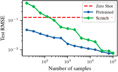
We find that this is indeed the case. We pretrain a spatiotemporal transformer model on a large amount of trajectories (100,000 each) with uniformly sampled coefficients ($v\in[-3,3],\ \delta\in[${10}^{-3}\text{\,}$,1.]$) generated from the advection and diffusion equations while finetuning on restricted samples from advection-diffusion simulations. The pretrained model is able to achieve much lower error with far fewer samples (Figure 1) despite the fact that it never saw advection and diffusion occurring in the same trajectory during pretraining.

To address question two, we must handle much larger spatial resolutions, varying scales, and heterogeneous relationships between fields. Over the rest of this section, we develop an approach for handling these challenges.

4.2 Architecture

Axial Attention

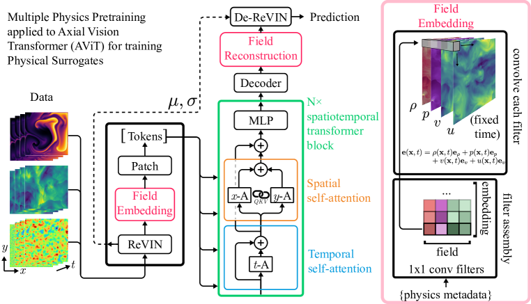
Given the success of large transformer models in other domains, we employ a scalable axial attention (Ho et al., 2019; Dong et al., 2022; Huang et al., 2019) transformer backbone. For a (2+1)-dimensional system with $T\times H\times W$ tokens, conventional dense attention attends over all tokens simultaneously and has cost $O((HWT)^{2})$. Axial attention instead performs a series of attention operations over each axis in turn, limiting the cost to $O(H^{2}+W^{2}+T^{2})$. In Figure 2, it can be seen that while we perform attention on each axis independently, spatial attention utilizes one set of linear projections for both the height (y) and width (x) axes.

Axial attention has been used in a number of video transformers (Arnab et al., 2021; Bertasius et al., 2021) due to the improved scalability in higher dimensions. While the tools used in our transformer backbone were introduced in prior work, our choice of using fully axial attention differs from ViViT which opted to only separate space and time attention. We favor scalability over maximizing accuracy and so chose the fully axial formulation. In subsequent sections we refer to this architecture as an Axial ViT (AViT).

Figure 2: (Left) MPP works by constructing a shared, normalized embedding space a single transformer backbone can process to produce predictions for multiple sets of physics. We use an AViT backbone which attends over space and time axis sequentially. Spatial attention is further split by axis, though these share linear projection weights. (Right) The field embedding and reconstruction filters are produced by sub-sampling channels from a larger $1\times 1$ convolutional filter.

Field Embedding and Normalization

Embedding multiple physical systems into a single shared representation is complicated by the fact that fields from different systems may operate on entirely different scales in terms of both magnitude and resolution. This is one of the primary challenges that must be addressed for multiple-physics pretraining.

To unify the magnitudes, we utilize reversible instance normalization (Kim et al., 2022). We compute the mean and standard deviation of each channel over the space-time dimensions and use them to normalize the input fields. These statistics are saved and used to denormalize the model outputs. While this approach was initially developed for time-series forecasting, the effect is similar to that reported in Subramanian et al. (2023), where it was found to be beneficial to rescale the inputs to a fixed norm during training.

After rescaling, the data is projected into a shared embedding space. This is the only component with weights that are unique to each source system. Given a system $S$ with state variables $u(x,t),\ v(x,t),\ p(x,t)\in\mathbb{R}$, we project each sample point or “pixel” into a space of dimension $D^{\mathrm{emb}}$:

$${\bm{e}}(x,t)=u(x,t){\bm{e}}_{u}+v(x,t){\bm{e}}_{v}+p(x,t){\bm{e}}_{p}$$ (2)

where ${\bm{e}}$ are embedding vectors in $\mathbb{R}^{D^{\mathrm{emb}}}$. This can be seen as a convolution with $1\times 1$ filters where the input channels of the filter are sub-selected to correspond to the fields present within a given dataset. On the right side of Figure 2, the filter is assembled by sub-selected columns of the larger filter corresponding to the provided fields. It is important to note that this initial projection setup is amenable to fine-tuning to unseen field types. This can be achieved by adding new channels to the initial embeddings, and training them from random initialization. In our models, the shared full resolution space is converted into patched tokens by a sequence of strided convolutions separated by pointwise nonlinearities as in Touvron et al. (2022).

The predictions are reconstructed from the processed tokens by reversing this process. The tokens are decoded by a sequence of transposed convolution blocks and projected onto the output fields by taking coordinate-wise inner products with reconstruction vectors ${\bm{r}}$:

$$u(x,t+\Delta t)=\langle{\bm{e}}(x,t+\Delta t),{\bm{r}}_{u}\rangle.$$ (3)

This can similarly be implemented as a $1\times 1$ convolution with the output channels of the convolution filter sub-selected. The mean and standard deviation computed from the inputs are then applied to these normalized outputs to produce the final de-normalized predictions as in Kim et al. (2022).

Position Biases and Boundaries

While in most cases, we would like the model to infer boundary conditions from the provided history, we make an exception to this policy for periodic boundaries as they change the continuity of the domain. Transformers are inherently permutation equivariant, and it is essential to include position biases so that the model can learn locality.

With a slight modification, we can use our position biases to capture the change in locality imposed by periodic boundaries. T5-style (Raffel et al., 2020) relative position encodings (RPE) utilize a lookup table to access learned embeddings corresponding to ranges of “relative distance”. For periodic boundary conditions, we modify the relative distance computation to account for neighbors across the periodic boundary. We find that this minor change enables generalization to periodic boundary conditions whether or not they are included in the training data.

4.3 Balancing Objectives During Training

Task Sampling

Our pretraining procedure operates on multiple levels of sampling. The task distribution varies in system $S$, spatial resolution $N_{S}$, and time resolution $T_{S}$ and we want diverse batches that accurately capture the signal this provides. However, sampling a full batch from multiple systems at different resolutions simultaneously would be inefficient on modern hardware as it would require batch processing of differently shaped tensors. Multi-GPU training adds an additional complication as the variance in execution time due to unbalanced workloads can lead to inefficient hardware usage.

Figure 3: Processing different physics (indicated by color) with different native resolutions incur varying wall-clock times (arrow lengths). To reduce the loss of GPU-cycles, we use gradient accumulation as a stochastic load-balancing mechanism, reducing the variance in work between all-reduce synchronizations.

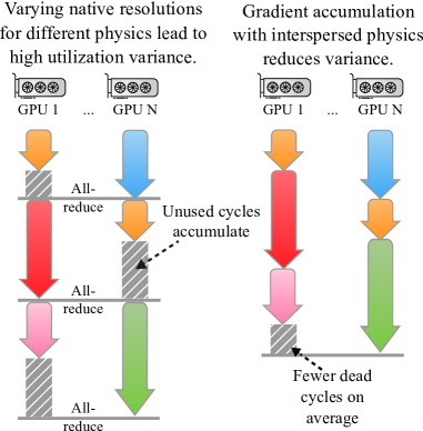
We mitigate both of these concerns with a simple randomization scheme involving gradient accumulation. Gradient accumulation utilizes multiple backward passes per synchronization step. We therefore sample a single system $S$ uniformly from $\mathcal{S}$ for each micro-batch. With $m$ micro-batches per synchronization step, we reduce the work-per-GPU variance $\sigma^{2}_{\mathcal{B}}$ to $\frac{1}{m}\sigma^{2}_{\mathcal{B}}$, significantly reducing the average lost cycles due to work discrepancies. This could likely be further reduced by an approximate packing problem solution (Cormen et al., 2022), but we found the random approach was sufficient for our needs. As we employ gradient accumulation in order to increase our batch sizes, this sampling procedure incurs no additional cost.

Scaled Training Objective

The simplest approach to obtaining updates from the different tasks is to add their gradients. However, as the magnitudes of the state variables can vary significantly between systems, unweighted losses will result in the gradients from the problems with the largest scales drowning out losses on smaller scales (Yu et al., 2020). To partially control this behavior, we train using the normalized MSE (NMSE) defined as:

$$\mathcal{L}_{\mathrm{NMSE}}=\frac{1}{|\mathcal{B}|}\sum_{S\in\mathcal{S}}\frac{\|\mathcal{M}({\bm{U}}_{t}^{S})-{\bm{u}}_{t+1}^{S}\|_{2}^{2}}{\|{\bm{u}}_{t+1}^{S}\|_{2}^{2}+\epsilon}$$ (4)

where $\mathcal{B}\subset\mathcal{S}$ denotes the micro-batch and $\epsilon$ is a small number added for numerical stability. This does not account for the full variation in difficulty. Even if sub-task losses have similar magnitudes at the start of training, it is possible for some systems to converge quickly while other losses remain high. Nonetheless, we found that this allows our training process to produce strong results on multiple systems simultaneously.

5 Experiments

We design our experiments to probe three vital questions about the utility of MPP:

1. Can large transformer models learn the dynamics of multiple physical systems simultaneously?

2. Does MPP provide a finetuning advantage over existing spatiotemporal foundation models for new autoregressive prediction tasks?

3. Are these learned representations useful for more than the autoregressive next-frame prediction task?

Data

We use the full collection of two-dimensional time-dependent simulations from PDEBench (Takamoto et al., 2022) as our primary source for diverse pretraining data. This includes systems governed by four unique nonlinear PDEs at a variety of state variables available, resolutions, initial conditions, boundary conditions, and simulation parameters. The specific PDEs are the compressible and incompressible Navier-Stokes equations, the shallow-water equations, and a 2D Diffusion-Reaction equation. Full details on the data used can be found in Appendix A.1.

Training settings

$T^{S}$ is fixed at 16 for all experiments as our VideoMAE comparison in Section 5.2 was unable to scale to larger sizes without gradient checkpointing. Autoregressive training is performed only one step ahead—no longer rollouts, noise corruption, or post-processing are included for stability. Training from scratch and MPP pretraining are always performed on the AViT architecture described in section 4.2. Full training details including data splits, optimization details, and hardware are documented in Appendix B.

5.1 Pretraining Performance

Table 1: NRMSE comparison between MPP-pretrained models and dedicated baselines. MPP-pretrained models learn multiple physical systems at least as well as standard baselines. Top performing within size range and overall are bolded. Dashes indicate precision not available. ^† While the PINN is much smaller, these models are fit per-example.

Model	$\#$Param	SWE	DiffRe2D	CNS M1.0	CNS M0.1
MPP-AViT-Ti	7.6M	0.0066	0.0168	0.0442	0.0312
UNet	7.7M	0.083-	0.84–	0.4725	1.6650
FNO	466K	0.0044	0.12–	0.1685	0.2425
PINN	8.5K†	0.017-	1.6—	—	—
ORCA-SWIN-B	88M	0.0060	0.82–	—	—
MPP-AViT-B	116M	0.0024	0.0106	0.0281	0.0172
MPP-AViT-S	29M	0.0039	0.0112	0.0319	0.0213
MPP-AViT-L	409M	0.0022	0.0098	0.0208	0.0147

Figure 4: Kinetic energy for representative incompressible training and compressible finetuning data. The “near” compressible snapshot resembles the training snapshot while “far” displays turbulent small scales not seen in the incompressible simulation.

First, we compare MPP-pretrained models to dedicated baselines from prior work across all available systems. The models are pretrained at a variety of sizes so we can begin to explore to benefits of scaling our approach. Precise model sizes can be found in Appendix B.1. Unlike the baselines which are trained on only one system and so must only learn one parameter regime, our models (denoted by MPP-AViT-*) must handle all all systems and regimes without finetuning. The effect of physical parameters, forcing, and simulation parameters must be inferred from context ${\bm{U}}^{S}_{t}$. The PINN (Raissi et al., 2019), UNet (Ronneberger et al., 2015), and FNO (Li et al., 2020) results are sourced from Takamoto et al. (2022) while the results from Shen et al. (2023) with a finetuned SWIN (Liu et al., 2021) are used for ORCA. Results are reported in terms of Normalized RMSE (NRMSE, the square root of Equation 4) averaged over fields and examples, as in Takamoto et al. (2023). Incompressible Navier-Stokes and more granular compressible Navier-Stokes results are reported in Appendix C.

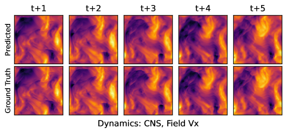
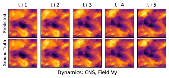
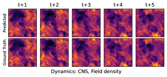
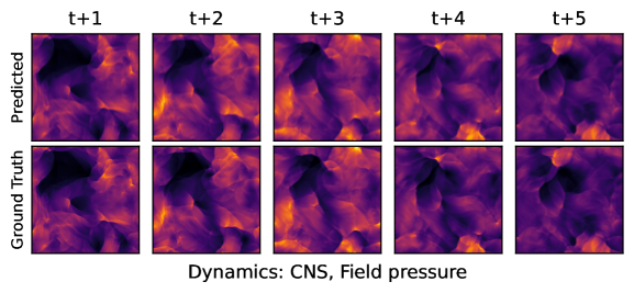
Our pretrained models are able achieve high-end performance on all datasets (Table 1) despite the difficulty of multi-task training (Yu et al., 2020). In fact, there is only one case where our pretrained models do not outperform all baselines. In some cases, the improvement over the baselines is nearly an order of magnitude in NRMSE and the performance improves with scale. However, we clarify that we are not claiming these results are optimal—we can, for instance, improve upon them by finetuning our own models on specific tasks. Rather, this experiment answers affirmatively that large transformers can learn multiple sets of dynamics simultaneously. Trajectories from pretrained models are displayed in Appendix C.2.

5.2 Transfer to Low-data Domains

Figure 5: NRMSE for transfer learning tasks. Solid lines are one-step error. Dashed lines are averaged error over five step rollouts. The MPP model shows clear performance benefits in both cases. The more turbulent behavior of “far” seems to be difficult to learn from scratch or from video data, but pretraining on physical data leads to much stronger results.

We remove all compressible fluid data from the training corpus and pretrain on the three remaining spatiotemporal systems. We evaluate transfer to two specific compressible Navier-Stokes datasets:

• “Near”: $M=0.1$, viscosity$=10^{-2}$, Random Periodic Initial Conditions

• “Far”: $M=1.0$, viscosity$=10^{-8}$, Turbulent Initial Conditions

Table 2: Memory usage during finetuning on 16$\times$3$\times$512$\times$512 inputs for batch size 1 using mixed precision.

Model	Max Memory
VideoMAE	79.3 GB
AViT-B	24.7 GB
AViT-Ti	6.7 GB
AViT-S	11.5 GB
AViT-L	59.7 GB

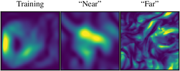
Snapshots of the kinetic energy for the finetuning systems and incompressible training data are visualized in Figure 4. While quantitatively evaluating the physics gap is an unsolved problem, the names reflect both prior physical knowledge and qualitative evaluation. “Near” features a low Mach number, the dimensionless quantity that correlates with compressible behavior, and viscosity similar to that of the incompressible simulation. ”Far“ has wildly different turbulent behavior that induces small scale structure never seen during training. However, despite the similarity in physical behavior, the simulations are still quite different: the compressible and incompressible simulations in PDEBench differ in spatial and temporal resolution, initial condition distribution, boundary conditions, viscosity, and velocity range in addition to the difference in compressibility. We use these sets to compare the finetuning performance of MPP, training from scratch, and an existing pretrained spatiotemporal transformer, VideoMAE (Tong et al., 2022) pretrained on both K400 (Kay et al., 2017) and SSV2 (Goyal et al., 2017) datasets.

Figure 5 shows that the MPP models outperform VideoMAE and training from scratch by a large margin in the low-data regime. Numerical results are listed in Appendix B. VideoMAE displays surprisingly strong finetuning performance given that the pretraining data is conventional video, but it is unable to match the much lower memory (Table 2) MPP-AViT-B in either setting. Predictably, both pretraining approaches are less accurate in the long-run on the turbulent “far” dataset. However, in the short-term the physical pretraining seems to provide an even larger advantage in this regime compared to the far smoother “near” data. Rollout visualizations are included in Appendix C.3.

5.3 Broader Usage of Pretrained Representations

One of the fascinating aspects of large pretrained models is the utility of their learned features for entirely new types of prediction problems. We explore this behavior with the inverse problem of parameter estimation for two parameters:

Forcing Identification for Incompressible Navier-Stokes We attempt to identify the constant forcing term used in the incompressible Navier-Stokes simulation from an input trajectory ${\bm{U}}_{t}^{S}$. We divide the validation set from pretraining, taking 1,000 trajectories as the new training set and using the rest for validation. Results are reported on the original test set.

Buoyancy for Incompressible Navier-Stokes For this, we turn to an additional fluid mechanics benchmark, PDEArena (Gupta & Brandstetter, 2022). This benchmark includes an incompressible Navier-Stokes simulation with variable buoyancy. Since this set was not used during training, we take 1,000 randomly sampled trajectories for train, 100 for validation, and a further 1,000 for testing.

Table 3: RMSE for inverse problem tasks. Error from constant prediction included for context.

Training	Forcing	Buoyancy
MPP	0.20$\pm.008$	0.78$\pm.006$
Scratch	0.43$\pm.012$	0.77$\pm.005$
Best Constant	1.00$\pm.000$	0.77$\pm.000$

We see mixed results (Table 3). Pretraining reduces the error in the forcing task by nearly half, but largely fails to outperform the optimal constant prediction in the buoyancy task. Prior work (Mialon et al., 2023) outperformed this constant prediction on buoyancy through Lie-transformation based contrastive pretraining using a convolutional architecture, so the task does appear to be possible. Since the AViT trained from scratch also fails to outperform a mean prediction, this is not a failure of MPP specifically, but it is an interesting observation. It is plausible that the use of the same attention weights in both spatial dimensions makes it difficult to disentangle directional magnitudes for scalar prediction. However, at this stage, it appears the MPP-pretrained model has significant advantages on the dense prediction task that strongly resembles the pretraining task, but no visible advantages for scalar prediction.

6 Conclusion

Limitations and Future Work

Creating a true foundation model for fluids, continuum mechanics, or general physics requires significantly more data diversity capturing far more behavior at resolutions that are practically useful to researchers in these fields than what is included in this paper. Additionally, the architecture used in our current work assumes uniformly gridded data. Training a foundation model that can be extended to engineering-grade problems requires the ability to handle highly non-uniform grids and arbitrary geometries. Nonetheless, this work addressed important roadblocks in the development of foundation models for these fields.

The worlds of science and engineering are filled with complex phenomena that could tremendously benefit from fast surrogates, but that are lacking sufficient data for training those surrogates. Our approach, Multiple Physics Pretraining, offers new opportunities for training highly transferable models for use in these settings. We demonstrated that transformers are able to be finetuned effectively when trained on partially overlapping physics. This suggests value in large pretrained models trained on diverse physics. Our experiments showed transformers pretrained with MPP learn multiple sets of physics competitively with many dedicated approaches and that this knowledge transfers even across significant physical gaps. As physical datasets for machine learning mature, this capability paves the way for the development of true foundation models for spatiotemporal physics.

Acknowledgments

The computations in this work were, in part, run at facilities supported by the Scientific Computing Core at the Flatiron Institute, a division of the Simons Foundation. M.P. is supported by the Department of Energy, Office of Science under contract number DE-AC02-05CH11231. M.M. would like to thank Jed Brown for his valuable insight on the simulation data.

Appendix A Data Details

A.1 PDEBench

To train and evaluate our models, we use the publicly available PDEBench dataset (Takamoto et al., 2022). We summarize the data included in this section. This dataset comprises a suite of time dependent and time independent simulations based on common PDE systems, generated with varying parameters, initial conditions, and boundary conditions. Specifically, PDEBench uses a discretized ground-truth solver with high precision to evolve the vector-valued solution to a given PDE at one time step to the solution at one time step later. When compiled across time steps, the vector-valued solutions take the form $x\in\mathbb{R}^{T\times C\times H\times W}$, where $T$ denotes the total number of times steps, $H$ and $W$ denote the spatial height and width of the simulation grid and $C$ denotes the parameter space representing the velocity ($v_{x}$ and $v_{y}$), pressure ($p$) and density ($\rho$) fields, such that $C=4$. For our study, we focus on the 2D fluid dynamics simulations in PDEBench. These are outlined loosely below; for more details, we refer the reader to Takamoto et al. (2022):

Compressible Navier-Stokes: These equations are used to model the pressure and velocity of both laminar and turbulent Newtonian fluids, and are applied to many real-world problems, from aerodynamics to interstellar gas dynamics. In the regime in which the density of the fluid can change due to pressure variation, the equations can be expressed:

$$\partial_{t}\rho+\nabla\cdot(\rho\mathbf{v}) =0,$$ (5)

$$\rho\left(\partial_{t}\mathbf{v}+\mathbf{v}\cdot\nabla\mathbf{v}\right) =-\nabla p+\eta\nabla^{2}\mathbf{v}+(\zeta+\eta/3)\nabla(\nabla\cdot\mathbf{v})$$ (6)

$$\partial_{t}(\epsilon+\rho v^{2}/2)+\nabla\cdot\left[(p+\epsilon+pv^{2}/2)\mathbf{v}-\mathbf{v}\cdot\bm{\sigma}^{\prime}\right] =\mathbf{0},$$ (7)

where $\rho$ is the fluid density, $\mathbf{v}$ is the fluid velocity, $p$ is the fluid pressure, $\epsilon$ is the internal energy, $\bm{\sigma}^{\prime}$ is the viscous stress tensor, $\eta$ is the shear viscosity, and $\zeta$ is the bulk viscosity. For our transfer experiments, we use the following two sets of data in particular:

1. A set of 1,000 trajectories on a $H\times W=512\times 512$ regular grid over $T=100$ time steps (where the separation between steps is $\Delta t=0.005$). Additionally, $(M,\eta,\zeta)=(1.0,10^{-8},10^{-8})$, where $M$, $\eta$, $\zeta$ denote the Mach number, the shear viscosity, and the bulk viscosity, respectively. The velocity field is initialized with a turbulent field, while the inital pressure and density fields are taken to be uniform.

2. A set of 10,000 trajectories on a $H\times W=128\times 128$ regular grid with $(M,\eta,\zeta)=(0.1,0.01,0.01)$. The time steps and initializations are as above.

Incompressible NS: In the incompressible regime, which typically occurs in fluids with low Mach numbers (as it rules out density and pressure waves like sound or shock waves), the Navier-Stokes equations simplify to:

$$\nabla\cdot\mathbf{v} =0,$$ (8)

$$\rho\left(\partial_{t}\mathbf{v}+\mathbf{v}\cdot\nabla\mathbf{v}\right) =-\nabla p+\eta\nabla^{2}\mathbf{v}+\mathbf{f},$$ (9)

where $\mathbf{v}$ is the velocity, $\rho$ is the density, $p$ is the pressure, $\eta$ is the viscosity, and $\mathbf{f}$ is the external force. The simulation in PDE bench is augmented by an immersed tracer that is transported by the velocity field:

$$\partial_{t}\rho_{smoke}=-\mathbf{v}\cdot\nabla\rho_{smoke}$$ (10)

These equations are typically used to model a variety of hydrodynamics systems such as weather. This data is produced at resolution $512\times 512$ with time step of $.0005$. The dataset contains a total of 1000 trajectories with 1000 time steps each.

Shallow water: In the event that the horizontal length scale of the fluid is significantly greater than the vertical length scale, the incompressible Navier-Stokes equations can be depth-integrated to derive the shallow water equations. These describe flow below a pressure surface in a fluid, and are given by

$$\partial_{t}h+\nabla\cdot(h\mathbf{v}) =0,$$ (11)

$$\partial_{t}(h\mathbf{v})+\nabla\cdot\left(\frac{1}{2}h\mathbf{v}^{2}+\frac{1}{2}g_{r}h^{2}\right) =-g_{r}h\nabla b,$$ (12)

where $h$ is the water depth, $\mathbf{v}$ is the velocity, $b$ is the bathymetry, and $g_{r}$ is the reduced gravity. For our data, we use 1,000 trajectories on a $H\times W=128\times 128$ regular grid over $T=100$ time steps. The specific simulation used is a 2D radial dam break scenario, where the water height is initialized as a circular bump in the center of the domain with a uniformly randomly sampled radius.

Diffusion-Reaction: The Diffusion-Reaction equations arise in systems with many interacting components and can be represented in the general form

$$\partial_{t}\mathbf{u}=\mathbf{D}\nabla^{2}\mathbf{u}+\mathbf{R}(\mathbf{u}),$$ (13)

where $\mathbf{u}$ is a vector of concentration variables, $\mathbf{D}$ is a diagonal matrix of diffusion coefficients, and $\mathbf{R}$ describes all local reaction kinetics. The most common application of diffusion-reaction equations is in chemical reactions, however they can also be used to describe a variety of dynamical processes. For our data, we use 1,000 trajectories on a $H\times W=128\times 128$ regular grid over $T=100$ time steps. The reaction functions for the activator and inhibitor are defined by the Fitzhugh-Nagumo equation (Klaasen & Troy, 1984), and their diffusion coefficients are $D_{u}=1\times 10^{-3}$ and $D_{v}=5\times 10^{-3}$ respectively. The initial conditions are generated as standard Gaussian random noise.

A.2 PDEArena

In addition to the 2D Incompressible Navier-Stokes data incorporated from PDEBench, we also include 2D Incompressible Navier-Stokes data from PDEArena (Gupta & Brandstetter, 2022). This includes a set of 5,200 training trajectories (and 1,300 validation and test trajectories each) on a $H\times W=128\times 128$ regular grid from which we take $T=16$ timesteps for prediction. As with the PDEBench simulations, the PDEArena simulations include a viscosity parameters of $\nu=0.01$ and Dirichlet boundary conditions, however they also include a buoyancy term $f\in[0.2,0.5]$ in the $y$ direction.

Appendix B Experiment Details

B.1 Model Configurations

The following architectural decisions were used across all AViT models trained in this paper:

• Pre/Post Norm: Pre-norm (Xiong et al., 2020)

• Normalization Type: Instance Normalization (Ulyanov et al., 2017)

• Activations: GeLU (Hendrycks & Gimpel, 2016)

• QK Norm: Yes (Dehghani et al., 2023)

• Patching: hMLP (Touvron et al., 2022)

• Decoder: Transposed hMLP (this is equivalent to the transposed convolutions mentioned in the main text).

• Causal Masking: False - We only evaluate the loss on the $T+1$ prediction.

Furthermore, we examine the performance of our models on the aforementioned PDE systems when the size of the model is scaled. Vision transformers have a variety of parameters that control the model’s size, including the number of processor blocks, the dimensionality of patch embeddings and self-attention, the dimensionality of Multi-Layer Perceptron (MLP) blocks, the number of attention heads, and the patch size applied on the input tensors. In previous studies on language (Hoffmann et al., 2022; Kaplan et al., 2020; Hernandez et al., 2021) and vision (Zhai et al., 2022), it has generally been noted that model performance is typically only weakly dependent on shape parameters, and instead depends largely on non-embedding parameter count given a fixed compute budget and dataset size. As such, we follow the general scaled architectures set forth by Zhai et al. (2022) for vision, and scale all aspects of the model shapes simultaneously to select a variety of model sizes for testing. These are detailed in 4.

Table 4: Details of the various model architectures and scales explored.

Model	Embed Dim.	MLP Dim.	# Heads	# Blocks	Patch Size	# Params
AViT-Ti	192	768	3	12	[16, 16]	7.6M
AViT-S	384	1536	6	12	[16, 16]	29M
AViT-B	768	3072	12	12	[16, 16]	116M
AViT-L	1024	4096	16	24	[16, 16]	409M

Software.

All model development and training in this paper is performed using PyTorch 2.0 (Paszke et al., 2019).

Hardware.

All training for both pretraining and finetuning is done using Distributed Data Parallel (DDP) across 8 Nvidia H100-80GB GPUs.

B.2 Exp 1: Pretraining Performance

For both MPP and scratch models, we train using the following settings:

• Training Duration: 200K steps

• Train/Val/Test: .8/.1/.1 split per dataset on the trajectory level.

• Task sampling: Uniformly sample task, then uniformly sample trajectory from task without replacement. We treat every 400 model updates (1 model update=5 micro-batches) as an “epoch” and reset the task pool.

• Micro-batch size: 8

• Accumulation Steps: 5

• Optimizer: Adan (Xie et al., 2023)

• Weight Decay: 1E-3

• Drop Path: 0.1

• Base LR: DAdaptation (Defazio & Mishchenko, 2023)

• LR Schedule: Cosine decay

• Gradient clipping: 1.0

Note, we use the automated learning selection strategy DAdaptation during pretraining runs in large part to avoid excessive hyperparameter tuning of our own models. In finetuning experiments, comparison models are tuned manually following the recommended settings from the model publishers to avoid differences being due to compatibility with the parameter-free method.

Data

For pretraining, we use all PDEBench datasets. These are described in Section A.1. In particular, we use the compressible and incompressible Navier-Stokes, Diffusion-Reaction 2D, and Shallow Water data.

B.3 Experiment 2: Transfer to Low-Data Domains

In this experiment, we compare the transferability of our MPP-Pretrained models to general-purposes pretrained video masked autoencoders (VideoMAE; Tong et al., 2022) for frame prediction on video-like PDEBench data (Takamoto et al., 2022).

For MPP and training from scatch, we use the following settings:

• Training Duration: 500 epochs

• Train/Val/Test: X/.1/.1 split per dataset on the trajectory level. Note that X is due to the fact that we test varying amounts of training data. These are subsampled from the training split of 80$\%$.

• Batch size: 8

• Accumulation Steps: 1 (No accumulation)

• Optimizer: Adan (Xie et al., 2023)

• Weight Decay: 1E-3

• Drop Path: 0.1

• Base LR: DAdaptation (Defazio & Mishchenko, 2023)

• LR Schedule: Cosine decay

• Gradient clipping: 1.0

Data

We study transferability of VideoMAE models for spatiotemporal prediction on video-like scientific data.

AViT Models are pretrained on datasets generated from three PDEs: Incompressible Navier-Stokes, Shallow Water, and Diffusion Reaction 2D.

We focus on transfer to the two datasets “Near” and “Far” (see Sect. 5.2) of fluid dynamics simulations taken from the PDEBench dataset (Takamoto et al., 2022). These simulations solve the compressible Navier-Stokes equations in a 2D geometry with periodic boundary conditions (see Appendix A.1 for additional details).

B.3.1 VideoMAE Settings

While VideoMAE does utilize spatiotemporal information, it was developed for a different setting, so we fully document all details of our adaptation of it here both for reproducibility and fairness in our comparison.

VideoMAE models are video transformers that were proven to be efficient data-learners for self-supervised video pretraining (Tong et al., 2022). They rely on an asymmetric encoder-decoder architecture building on a vanilla ViT backbone with joint space-time attention. VideoMAE models are pretrained by learning to reconstruct masked videos using a random tube-masking strategy with a extremely high masking ratio ($\sim$ 90 %).

We make use of two publicly available models, hereafter called VideoMAE-K400 and VideoMAE-SSV2, that were pretrained on Kinetics-400 dataset (K400; Kay et al., 2017) and Something-Something V2 dataset (SSV2; Goyal et al., 2017), respectively. Both datasets are made of short videos (typically $\leq 10\,s$ long) of human-object or human-human interactions. VideoMAE-K400 (respectively, VideoMAE-SSV2) was pretrained on $\sim$ 240k ($\sim$ 170k) videos. We focus on the models that build on a ViT-base backbone, so that their size (in terms of number of trainable parameters) remains comparable to that of MPP-AViT-B. After adaptation of the input and output linear layers as described below, the number of trainable parameters of these models reaches $\sim 95$ M.

Number of channels.

Same as the original pretraining procedure, the input data $x\in\mathbb{R}^{C\times T\times H\times W}$ is divided into non-overlapping joint space-time cubes of size $2\times 16\times 16$. These are embedded through a Conv3d layer, resulting in $\frac{T}{2}\times\frac{H}{16}\times\frac{W}{16}$ tokens. Since our PDEBench data has $C=4$ channels instead of 3 for the RGB videos from the pretraining set, we had to adapt the number of input channels of this Conv3d layer accordingly. The weights of this new layer were defined using a (rescaled) repetition of the pretrained weights from the original layer. Similarly, the output number of features of the final linear projection layer of the model had to be adapted to $C=4$ channels. The weights and biases of this layer were extended by consistently repeating the original pretrained weights and biases.

Positional encoding.

The number of tokens resulting from our PDEBench data did not match the number of tokens resulting from the pretraining datasets. Consequently, we also had to adapt the pretraining positional encoding. We chose to interpolate accordingly the original 1D sine/cosine positional encoding (Vaswani et al., 2017) using a trilinear interpolation after having reshaped the token index axis onto a 3D grid.

B.3.2 Video MAE Finetuning Procedure

We describe the finetuning procedure of the pretrained VideoMAE models for frame prediction. Frame prediction consists in predicting the next $T_{p}$ frames of a video given a context of $T_{c}$ frames. Since the pretrained models manipulates space-time cubes of size 2 in time, we naturally choose $T_{p}=2$. The context size is taken to be $T_{c}=16$ for consistency with MPP-AViT models. We finetune the pretrained models for frame prediction by adapting the self-supervised training strategy in order to reconstruct the last $T_{p}$ frames of a masked video of $T=T_{c}+T_{p}$ frames.

Masking strategy.

For frame prediction, instead of the random tube-masking strategy, we simply mask the last $T_{p}$ frames of the input data.

Loss.

We finetune our models by minimizing a NMSE loss. In this context, denoting by ${x,y\in\mathbb{R}^{C\times T_{p}\times H\times W}}$ the output of our model and the target (masked frames), respectively, the NMSE loss is defined by $\mathcal{L}(x,y)=\sum_{c=1}^{C}\sum_{t=1}^{T_{p}}\lVert x_{c,t}-y_{c,t}\rVert_{2}^{2}/\lVert y_{c,t}\rVert_{2}^{2}$.

Normalization of the data.

Each set of PDEBench simulations is globally and channel-wise rescaled so that pixel values all fit in $[0,1]$. Additionally, we normalize channel-wise the targets $y\in\mathbb{R}^{C\times T_{p}\times H\times W}$ by subtracting the global mean of the corresponding context frames and then dividing by their global standard deviation.

Optimization.

We finetune the pretrained models over 500 epochs and a (total) batch size of 8 using AdamW optimizer (Loshchilov & Hutter, 2019). Except for the learning rate, the remaining optimization hyperparameters are chosen to be consistent with those used in the finetuning experiments of Tong et al. (2022) (Table 10). In particular, we choose a weight decay $\lambda=0.05$, $(\beta_{1},\beta_{2})=(0.9,0.999)$, a cosine learning rate decay scheduler with 5 warmup epochs, a drop path rate of 0.1, and a layer-wise learning rate decay parametrized by 0.75. In this setting, the learning rate is adjusted by performing a hyperparameter search monitored with WandB (Biewald, 2020). We report the resulting optimal values per pretrained model and dataset in Table 5.

Table 5: Effective learning rate for the finetuning of VideoMAE.

	“Near”	“Far”
VideoMAE (K400)	0.00039	0.00198
VideoMAE (SSV2)	0.00186	0.00150

B.4 Exp 3: Broader Usage of Pretrained Representations

For MPP and training from scatch, we use the following settings:

• Training Duration: 500 epochs

• Train/Val/Test: 1000/100/1000 taken from original validation set or randomly depending on whether data was used for training.

• Batch size: 24

• Accumulation Steps: 1 (No accumulation)

• Optimizer: Adan (Xie et al., 2023)

• Weight Decay: 1E-3

• Drop Path: 0.1

• Base LR: DAdaptation (Defazio & Mishchenko, 2023)

• LR Schedule: Cosine decay

• Gradient clipping: 1.0

Appendix C Extended Results

C.1 Exp2: Numerical Results

We provide numerical results corresponding to Figure 5 in Tables 6 and 7. We refer to Sect. 5.2 for discussion.

Table 6: Test NRMSE for “Near” Compressible Navier-Stokes M0.1, $\eta=.01$.

	$\#$ Training Samples (NRMSE $\times 10^{-1}$)
Model	100		200		400		600		800
	T+1	T+5	T+1	T+5	T+1	T+5	T+1	T+5	T+1	T+5
VideoMAE (K400)	1.26	1.98	0.78	1.25	0.49	0.83	0.39	0.62	0.33	0.50
VideoMAE (SSV2)	0.95	1.61	0.63	1.04	0.42	0.66	0.33	0.52	0.25	0.39
MPP-AViT-B	0.66	1.13	0.42	0.81	0.27	0.55	0.22	0.35	0.19	0.30

Table 7: Test NRMSE for “Far” Compressible Navier-Stokes

	$\#$ Training Samples (NRMSE $\times 10^{-1}$)
Model	100		200		400		600		800
	T+1	T+5	T+1	T+5	T+1	T+5	T+1	T+5	T+1	T+5
VideoMAE (K400)	1.16	1.60	0.79	1.10	0.73	0.96	0.53	0.70	0.49	0.65
VideoMAE (SSV2)	0.98	1.42	0.75	1.03	0.62	0.84	0.55	0.74	0.51	0.67
MPP-AViT-B	0.60	1.15	0.37	0.77	0.27	0.66	.32	0.63	0.24	0.48

C.2 Pretraining Trajectories

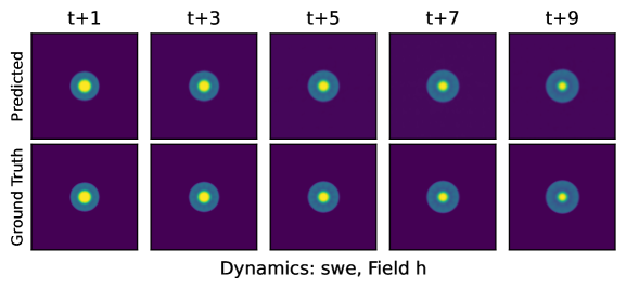
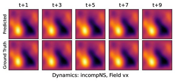
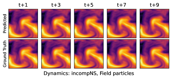
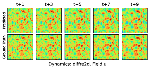
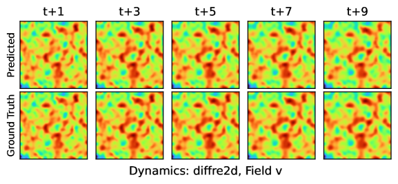
Here we show example trajectories from pretrained models. Videos are included in the attached supplementary material. After pretraining, we find that the model initially produces strong predictions, but patch artifacts creep in over time.

Figure 6: Pretraining trajectory.

Figure 7: Pretraining trajectory.

Figure 8: Pretraining trajectory.

Figure 9: Pretraining trajectory.

Figure 10: Pretraining trajectory.

C.3 Finetuning Trajectories

After finetuning, we find that the patch-based instability mostly disappears. Again, videos displaying longer trajectories are available in the supplementary material.

Figure 11: Finetuning trajectory.

Figure 12: Finetuning trajectory.

Figure 13: Finetuning trajectory.

Figure 14: Finetuning trajectory.

References

- Arnab et al. (2021) Anurag Arnab, Mostafa Dehghani, Georg Heigold, Chen Sun, Mario Lučić, and Cordelia Schmid. Vivit: A video vision transformer, 2021.
- Balestriero et al. (2023) Randall Balestriero, Mark Ibrahim, Vlad Sobal, Ari Morcos, Shashank Shekhar, Tom Goldstein, Florian Bordes, Adrien Bardes, Gregoire Mialon, Yuandong Tian, Avi Schwarzschild, Andrew Gordon Wilson, Jonas Geiping, Quentin Garrido, Pierre Fernandez, Amir Bar, Hamed Pirsiavash, Yann LeCun, and Micah Goldblum. A cookbook of self-supervised learning, 2023.
- Bar & Sochen (2019) Leah Bar and Nir Sochen. Unsupervised deep learning algorithm for pde-based forward and inverse problems. arXiv preprint arXiv:1904.05417, 2019.
- Ben-Bouallegue et al. (2023) Zied Ben-Bouallegue, Mariana C A Clare, Linus Magnusson, Estibaliz Gascon, Michael Maier-Gerber, Martin Janousek, Mark Rodwell, Florian Pinault, Jesper S Dramsch, Simon T K Lang, Baudouin Raoult, Florence Rabier, Matthieu Chevallier, Irina Sandu, Peter Dueben, Matthew Chantry, and Florian Pappenberger. The rise of data-driven weather forecasting, 2023.
- Bertasius et al. (2021) Gedas Bertasius, Heng Wang, and Lorenzo Torresani. Is space-time attention all you need for video understanding? In Proceedings of the International Conference on Machine Learning (ICML), July 2021.
- Bi et al. (2023) Kaifeng Bi, Lingxi Xie, Hengheng Zhang, Xin Chen, Xiaotao Gu, and Qi Tian. Accurate medium-range global weather forecasting with 3d neural networks. Nature, 619(7970):533–538, 2023.
- Biewald (2020) Lukas Biewald. Experiment tracking with weights and biases, 2020. URL https://www.wandb.com/. Software available from wandb.com.
- Bommasani et al. (2021) Rishi Bommasani, Drew A Hudson, Ehsan Adeli, Russ Altman, Simran Arora, Sydney von Arx, Michael S Bernstein, Jeannette Bohg, Antoine Bosselut, Emma Brunskill, et al. On the opportunities and risks of foundation models. arXiv preprint arXiv:2108.07258, 2021.
- Bran et al. (2023) Andres M Bran, Sam Cox, Andrew D White, and Philippe Schwaller. Chemcrow: Augmenting large-language models with chemistry tools, 2023.
- Brown et al. (2020) Tom Brown, Benjamin Mann, Nick Ryder, Melanie Subbiah, Jared D Kaplan, Prafulla Dhariwal, Arvind Neelakantan, Pranav Shyam, Girish Sastry, Amanda Askell, et al. Language models are few-shot learners. Advances in neural information processing systems, 33:1877–1901, 2020.
- Bruna et al. (2022) Joan Bruna, Benjamin Peherstorfer, and Eric Vanden-Eijnden. Neural galerkin scheme with active learning for high-dimensional evolution equations, 2022.
- Cao (2021) Shuhao Cao. Choose a transformer: Fourier or galerkin, 2021.
- Chen et al. (2020) Ting Chen, Simon Kornblith, Mohammad Norouzi, and Geoffrey Hinton. A simple framework for contrastive learning of visual representations, 2020.
- Chithrananda et al. (2020) Seyone Chithrananda, Gabriel Grand, and Bharath Ramsundar. Chemberta: Large-scale self-supervised pretraining for molecular property prediction, 2020.
- Cormen et al. (2022) Thomas H Cormen, Charles E Leiserson, Ronald L Rivest, and Clifford Stein. Introduction to algorithms. MIT press, 2022.
- Cranmer et al. (2021) Miles Cranmer, Daniel Tamayo, Hanno Rein, Peter Battaglia, Samuel Hadden, Philip J. Armitage, Shirley Ho, and David N. Spergel. A bayesian neural network predicts the dissolution of compact planetary systems. Proceedings of the National Academy of Sciences, 118(40):e2026053118, 2021. doi: 10.1073/pnas.2026053118. URL https://www.pnas.org/doi/abs/10.1073/pnas.2026053118.
- Dang et al. (2022) Yuchen Dang, Zheyuan Hu, Miles Cranmer, Michael Eickenberg, and Shirley Ho. Tnt: Vision transformer for turbulence simulations, 2022.
- Defazio & Mishchenko (2023) Aaron Defazio and Konstantin Mishchenko. Learning-rate-free learning by d-adaptation, 2023.
- Dehghani et al. (2023) Mostafa Dehghani, Josip Djolonga, Basil Mustafa, Piotr Padlewski, Jonathan Heek, Justin Gilmer, Andreas Steiner, Mathilde Caron, Robert Geirhos, Ibrahim Alabdulmohsin, Rodolphe Jenatton, Lucas Beyer, Michael Tschannen, Anurag Arnab, Xiao Wang, Carlos Riquelme, Matthias Minderer, Joan Puigcerver, Utku Evci, Manoj Kumar, Sjoerd van Steenkiste, Gamaleldin F. Elsayed, Aravindh Mahendran, Fisher Yu, Avital Oliver, Fantine Huot, Jasmijn Bastings, Mark Patrick Collier, Alexey Gritsenko, Vighnesh Birodkar, Cristina Vasconcelos, Yi Tay, Thomas Mensink, Alexander Kolesnikov, Filip Pavetić, Dustin Tran, Thomas Kipf, Mario Lučić, Xiaohua Zhai, Daniel Keysers, Jeremiah Harmsen, and Neil Houlsby. Scaling vision transformers to 22 billion parameters, 2023.
- Desai et al. (2022) Shaan Desai, Marios Mattheakis, Hayden Joy, Pavlos Protopapas, and Stephen Roberts. One-shot transfer learning of physics-informed neural networks, 2022.
- Devlin et al. (2018) Jacob Devlin, Ming-Wei Chang, Kenton Lee, and Kristina Toutanova. Bert: Pre-training of deep bidirectional transformers for language understanding. arXiv preprint arXiv:1810.04805, 2018.
- Dong et al. (2022) Xiaoyi Dong, Jianmin Bao, Dongdong Chen, Weiming Zhang, Nenghai Yu, Lu Yuan, Dong Chen, and Baining Guo. Cswin transformer: A general vision transformer backbone with cross-shaped windows, 2022.
- Dresdner et al. (2023) Gideon Dresdner, Dmitrii Kochkov, Peter Christian Norgaard, Leonardo Zepeda-Nunez, Jamie Smith, Michael Brenner, and Stephan Hoyer. Learning to correct spectral methods for simulating turbulent flows. Transactions on Machine Learning Research, 2023. ISSN 2835-8856. URL https://openreview.net/forum?id=wNBARGxoJn.
- Duraisamy et al. (2019) Karthik Duraisamy, Gianluca Iaccarino, and Heng Xiao. Turbulence modeling in the age of data. Annual Review of Fluid Mechanics, 51(1):357–377, jan 2019. doi: 10.1146/annurev-fluid-010518-040547. URL https://doi.org/10.1146%2Fannurev-fluid-010518-040547.
- Farlow (1993) Stanley J Farlow. Partial differential equations for scientists and engineers. Courier Corporation, 1993.
- Goswami et al. (2022) Somdatta Goswami, Katiana Kontolati, Michael D Shields, and George Em Karniadakis. Deep transfer operator learning for partial differential equations under conditional shift. Nature Machine Intelligence, 4(12):1155–1164, 2022.
- Goyal et al. (2017) Raghav Goyal, Samira Ebrahimi Kahou, Vincent Michalski, Joanna Materzyńska, Susanne Westphal, Heuna Kim, Valentin Haenel, Ingo Fruend, Peter Yianilos, Moritz Mueller-Freitag, Florian Hoppe, Christian Thurau, Ingo Bax, and Roland Memisevic. The ”something something” video database for learning and evaluating visual common sense, 2017.
- Grossmann et al. (2023) Tamara G. Grossmann, Urszula Julia Komorowska, Jonas Latz, and Carola-Bibiane Schönlieb. Can physics-informed neural networks beat the finite element method?, 2023.
- Gupta & Brandstetter (2022) Jayesh K Gupta and Johannes Brandstetter. Towards multi-spatiotemporal-scale generalized pde modeling. arXiv preprint arXiv:2209.15616, 2022.
- Han et al. (2018) Jiequn Han, Arnulf Jentzen, and Weinan E. Solving high-dimensional partial differential equations using deep learning. Proceedings of the National Academy of Sciences, 115(34):8505–8510, 2018.
- He et al. (2021) Kaiming He, Xinlei Chen, Saining Xie, Yanghao Li, Piotr Dollár, and Ross Girshick. Masked autoencoders are scalable vision learners, 2021.
- He et al. (2019) Siyu He, Yin Li, Yu Feng, Shirley Ho, Siamak Ravanbakhsh, Wei Chen, and Barnabás Póczos. Learning to predict the cosmological structure formation. Proceedings of the National Academy of Sciences, 116(28):13825–13832, 2019. doi: 10.1073/pnas.1821458116. URL https://www.pnas.org/doi/abs/10.1073/pnas.1821458116.
- Hendrycks & Gimpel (2016) Dan Hendrycks and Kevin Gimpel. Gaussian error linear units (gelus), 2016.
- Hernandez et al. (2021) Danny Hernandez, Jared Kaplan, Tom Henighan, and Sam McCandlish. Scaling laws for transfer. arXiv preprint arXiv:2102.01293, 2021.
- Ho et al. (2019) Jonathan Ho, Nal Kalchbrenner, Dirk Weissenborn, and Tim Salimans. Axial attention in multidimensional transformers, 2019.
- Hoffmann et al. (2022) Jordan Hoffmann, Sebastian Borgeaud, Arthur Mensch, Elena Buchatskaya, Trevor Cai, Eliza Rutherford, Diego de Las Casas, Lisa Anne Hendricks, Johannes Welbl, Aidan Clark, et al. Training compute-optimal large language models. arXiv preprint arXiv:2203.15556, 2022.
- Huang et al. (2019) Zilong Huang, Xinggang Wang, Lichao Huang, Chang Huang, Yunchao Wei, and Wenyu Liu. Ccnet: Criss-cross attention for semantic segmentation. In Proceedings of the IEEE/CVF International Conference on Computer Vision, pp. 603–612, 2019.
- Jamieson et al. (2023) Drew Jamieson, Yin Li, Renan Alves de Oliveira, Francisco Villaescusa-Navarro, Shirley Ho, and David N Spergel. Field-level neural network emulator for cosmological n-body simulations. The Astrophysical Journal, 952(2):145, 2023.
- Jiang et al. (2023) Lavender Yao Jiang, Xujin Chris Liu, Nima Pour Nejatian, Mustafa Nasir-Moin, Duo Wang, Anas Abidin, Kevin Eaton, Howard Antony Riina, Ilya Laufer, Paawan Punjabi, et al. Health system-scale language models are all-purpose prediction engines. Nature, pp. 1–6, 2023.
- Kaplan et al. (2020) Jared Kaplan, Sam McCandlish, Tom Henighan, Tom B Brown, Benjamin Chess, Rewon Child, Scott Gray, Alec Radford, Jeffrey Wu, and Dario Amodei. Scaling laws for neural language models. arXiv preprint arXiv:2001.08361, 2020.
- Kay et al. (2017) Will Kay, Joao Carreira, Karen Simonyan, Brian Zhang, Chloe Hillier, Sudheendra Vijayanarasimhan, Fabio Viola, Tim Green, Trevor Back, Paul Natsev, Mustafa Suleyman, and Andrew Zisserman. The kinetics human action video dataset, 2017.
- Kim et al. (2022) Taesung Kim, Jinhee Kim, Yunwon Tae, Cheonbok Park, Jang-Ho Choi, and Jaegul Choo. Reversible instance normalization for accurate time-series forecasting against distribution shift. In International Conference on Learning Representations, 2022. URL https://openreview.net/forum?id=cGDAkQo1C0p.
- Klaasen & Troy (1984) Gene A Klaasen and William C Troy. Stationary wave solutions of a system of reaction-diffusion equations derived from the fitzhugh–nagumo equations. SIAM Journal on Applied Mathematics, 44(1):96–110, 1984.
- Kochkov et al. (2021) Dmitrii Kochkov, Jamie A. Smith, Ayya Alieva, Qing Wang, Michael P. Brenner, and Stephan Hoyer. Machine learning–accelerated computational fluid dynamics. Proceedings of the National Academy of Sciences, 118(21):e2101784118, 2021. doi: 10.1073/pnas.2101784118. URL https://www.pnas.org/doi/abs/10.1073/pnas.2101784118.
- Kovachki et al. (2023) Nikola Kovachki, Zongyi Li, Burigede Liu, Kamyar Azizzadenesheli, Kaushik Bhattacharya, Andrew Stuart, and Anima Anandkumar. Neural operator: Learning maps between function spaces, 2023.
- Leung & Bovy (2023) Henry W. Leung and Jo Bovy. Towards an astronomical foundation model for stars with a transformer-based model, 2023.
- Li et al. (2020) Zongyi Li, Nikola Kovachki, Kamyar Azizzadenesheli, Burigede Liu, Kaushik Bhattacharya, Andrew Stuart, and Anima Anandkumar. Fourier neural operator for parametric partial differential equations. arXiv preprint arXiv:2010.08895, 2020.
- Li et al. (2021) Zongyi Li, Hongkai Zheng, Nikola Kovachki, David Jin, Haoxuan Chen, Burigede Liu, Kamyar Azizzadenesheli, and Anima Anandkumar. Physics-informed neural operator for learning partial differential equations. arXiv preprint arXiv:2111.03794, 2021.
- Liu et al. (2021) Ze Liu, Yutong Lin, Yue Cao, Han Hu, Yixuan Wei, Zheng Zhang, Stephen Lin, and Baining Guo. Swin transformer: Hierarchical vision transformer using shifted windows. In Proceedings of the IEEE/CVF International Conference on Computer Vision (ICCV), 2021.
- Loshchilov & Hutter (2019) Ilya Loshchilov and Frank Hutter. Decoupled weight decay regularization. In International Conference on Learning Representations, 2019. URL https://openreview.net/forum?id=Bkg6RiCqY7.
- Lu et al. (2019) Lu Lu, Pengzhan Jin, and George Em Karniadakis. Deeponet: Learning nonlinear operators for identifying differential equations based on the universal approximation theorem of operators. arXiv preprint arXiv:1910.03193, 2019.
- Lusch et al. (2018) Bethany Lusch, J. Nathan Kutz, and Steven L. Brunton. Deep learning for universal linear embeddings of nonlinear dynamics. Nature Communications, 9(1):4950, 2018. doi: 10.1038/s41467-018-07210-0. URL https://doi.org/10.1038/s41467-018-07210-0.
- Mialon et al. (2023) Grégoire Mialon, Quentin Garrido, Hannah Lawrence, Danyal Rehman, Yann LeCun, and Bobak T. Kiani. Self-supervised learning with lie symmetries for partial differential equations, 2023.
- Nguyen et al. (2023a) Tuan Dung Nguyen, Yuan-Sen Ting, Ioana Ciucă, Charlie O’Neill, Ze-Chang Sun, Maja Jabłońska, Sandor Kruk, Ernest Perkowski, Jack Miller, Jason Li, Josh Peek, Kartheik Iyer, Tomasz Różański, Pranav Khetarpal, Sharaf Zaman, David Brodrick, Sergio J. Rodríguez Méndez, Thang Bui, Alyssa Goodman, Alberto Accomazzi, Jill Naiman, Jesse Cranney, Kevin Schawinski, and UniverseTBD. Astrollama: Towards specialized foundation models in astronomy, 2023a.
- Nguyen et al. (2023b) Tung Nguyen, Johannes Brandstetter, Ashish Kapoor, Jayesh K Gupta, and Aditya Grover. Climax: A foundation model for weather and climate. arXiv preprint arXiv:2301.10343, 2023b.
- Paszke et al. (2019) Adam Paszke, Sam Gross, Francisco Massa, Adam Lerer, James Bradbury, Gregory Chanan, Trevor Killeen, Zeming Lin, Natalia Gimelshein, Luca Antiga, Alban Desmaison, Andreas Kopf, Edward Yang, Zachary DeVito, Martin Raison, Alykhan Tejani, Sasank Chilamkurthy, Benoit Steiner, Lu Fang, Junjie Bai, and Soumith Chintala. Pytorch: An imperative style, high-performance deep learning library. In H. Wallach, H. Larochelle, A. Beygelzimer, F. d'Alché-Buc, E. Fox, and R. Garnett (eds.), Advances in Neural Information Processing Systems, volume 32. Curran Associates, Inc., 2019. URL https://proceedings.neurips.cc/paper_files/paper/2019/file/bdbca288fee7f92f2bfa9f7012727740-Paper.pdf.
- Pathak et al. (2022) Jaideep Pathak, Shashank Subramanian, Peter Harrington, Sanjeev Raja, Ashesh Chattopadhyay, Morteza Mardani, Thorsten Kurth, David Hall, Zongyi Li, Kamyar Azizzadenesheli, Pedram Hassanzadeh, Karthik Kashinath, and Animashree Anandkumar. Fourcastnet: A global data-driven high-resolution weather model using adaptive fourier neural operators. arXiv preprint arXiv:2202.11214, 2022.
- Pfaff et al. (2021) Tobias Pfaff, Meire Fortunato, Alvaro Sanchez-Gonzalez, and Peter Battaglia. Learning mesh-based simulation with graph networks. In International Conference on Learning Representations, 2021. URL https://openreview.net/forum?id=roNqYL0_XP.
- Rackauckas et al. (2021) Christopher Rackauckas, Yingbo Ma, Julius Martensen, Collin Warner, Kirill Zubov, Rohit Supekar, Dominic Skinner, Ali Ramadhan, and Alan Edelman. Universal differential equations for scientific machine learning, 2021.
- Radford et al. (2018) Alec Radford, Karthik Narasimhan, Tim Salimans, Ilya Sutskever, et al. Improving language understanding by generative pre-training. 2018.
- Radford et al. (2019) Alec Radford, Jeffrey Wu, Rewon Child, David Luan, Dario Amodei, Ilya Sutskever, et al. Language models are unsupervised multitask learners. OpenAI blog, 1(8):9, 2019.
- Raffel et al. (2020) Colin Raffel, Noam Shazeer, Adam Roberts, Katherine Lee, Sharan Narang, Michael Matena, Yanqi Zhou, Wei Li, and Peter J. Liu. Exploring the limits of transfer learning with a unified text-to-text transformer, 2020.
- Raissi et al. (2019) Maziar Raissi, Paris Perdikaris, and George E Karniadakis. Physics-informed neural networks: A deep learning framework for solving forward and inverse problems involving nonlinear partial differential equations. Journal of Computational physics, 378:686–707, 2019.
- Ronneberger et al. (2015) Olaf Ronneberger, Philipp Fischer, and Thomas Brox. U-net: Convolutional networks for biomedical image segmentation. In Medical Image Computing and Computer-Assisted Intervention–MICCAI 2015: 18th International Conference, Munich, Germany, October 5-9, 2015, Proceedings, Part III 18, pp. 234–241. Springer, 2015.
- Shen et al. (2023) Junhong Shen, Liam Li, Lucio M. Dery, Corey Staten, Mikhail Khodak, Graham Neubig, and Ameet Talwalkar. Cross-modal fine-tuning: Align then refine, 2023. URL https://arxiv.org/abs/2302.05738.
- Sirignano & MacArt (2023) Justin Sirignano and Jonathan F. MacArt. Deep learning closure models for large-eddy simulation of flows around bluff bodies. Journal of Fluid Mechanics, 966, jul 2023. doi: 10.1017/jfm.2023.446. URL https://doi.org/10.1017%2Fjfm.2023.446.
- Sirignano & Spiliopoulos (2018) Justin Sirignano and Konstantinos Spiliopoulos. Dgm: A deep learning algorithm for solving partial differential equations. Journal of computational physics, 375:1339–1364, 2018.
- Stachenfeld et al. (2022) Kimberly Stachenfeld, Drummond B. Fielding, Dmitrii Kochkov, Miles Cranmer, Tobias Pfaff, Jonathan Godwin, Can Cui, Shirley Ho, Peter Battaglia, and Alvaro Sanchez-Gonzalez. Learned coarse models for efficient turbulence simulation, 2022.
- Subel et al. (2023) Adam Subel, Yifei Guan, Ashesh Chattopadhyay, and Pedram Hassanzadeh. Explaining the physics of transfer learning in data-driven turbulence modeling. PNAS nexus, 2(3):pgad015, 2023.
- Subramanian et al. (2023) Shashank Subramanian, Peter Harrington, Kurt Keutzer, Wahid Bhimji, Dmitriy Morozov, Michael Mahoney, and Amir Gholami. Towards foundation models for scientific machine learning: Characterizing scaling and transfer behavior, 2023.
- Takamoto et al. (2022) Makoto Takamoto, Timothy Praditia, Raphael Leiteritz, Dan MacKinlay, Francesco Alesiani, Dirk Pflüger, and Mathias Niepert. PDEBench: An Extensive Benchmark for Scientific Machine Learning. In 36th Conference on Neural Information Processing Systems (NeurIPS 2022) Track on Datasets and Benchmarks, 2022. URL https://arxiv.org/abs/2210.07182.
- Takamoto et al. (2023) Makoto Takamoto, Francesco Alesiani, and Mathias Niepert. Learning neural pde solvers with parameter-guided channel attention, 2023.
- Tong et al. (2022) Zhan Tong, Yibing Song, Jue Wang, and Limin Wang. VideoMAE: Masked autoencoders are data-efficient learners for self-supervised video pre-training. In Alice H. Oh, Alekh Agarwal, Danielle Belgrave, and Kyunghyun Cho (eds.), Advances in Neural Information Processing Systems, 2022. URL https://openreview.net/forum?id=AhccnBXSne.
- Touvron et al. (2022) Hugo Touvron, Matthieu Cord, Alaaeldin El-Nouby, Jakob Verbeek, and Herve Jegou. Three things everyone should know about vision transformers. arXiv preprint arXiv:2203.09795, 2022.
- Tu et al. (2023) Tao Tu, Shekoofeh Azizi, Danny Driess, Mike Schaekermann, Mohamed Amin, Pi-Chuan Chang, Andrew Carroll, Chuck Lau, Ryutaro Tanno, Ira Ktena, Basil Mustafa, Aakanksha Chowdhery, Yun Liu, Simon Kornblith, David Fleet, Philip Mansfield, Sushant Prakash, Renee Wong, Sunny Virmani, Christopher Semturs, S Sara Mahdavi, Bradley Green, Ewa Dominowska, Blaise Aguera y Arcas, Joelle Barral, Dale Webster, Greg S. Corrado, Yossi Matias, Karan Singhal, Pete Florence, Alan Karthikesalingam, and Vivek Natarajan. Towards generalist biomedical ai, 2023.
- Ulyanov et al. (2017) Dmitry Ulyanov, Andrea Vedaldi, and Victor Lempitsky. Instance normalization: The missing ingredient for fast stylization, 2017.
- Um et al. (2021) Kiwon Um, Robert Brand, Yun, Fei, Philipp Holl, and Nils Thuerey. Solver-in-the-loop: Learning from differentiable physics to interact with iterative pde-solvers, 2021.
- Vaswani et al. (2017) Ashish Vaswani, Noam Shazeer, Niki Parmar, Jakob Uszkoreit, Llion Jones, Aidan N Gomez, Łukasz Kaiser, and Illia Polosukhin. Attention is all you need. Advances in neural information processing systems, 30, 2017.
- Wang et al. (2022) Hengjie Wang, Robert Planas, Aparna Chandramowlishwaran, and Ramin Bostanabad. Mosaic flows: A transferable deep learning framework for solving pdes on unseen domains. Computer Methods in Applied Mechanics and Engineering, 389:114424, 2022.
- Wei et al. (2022) Jason Wei, Yi Tay, Rishi Bommasani, Colin Raffel, Barret Zoph, Sebastian Borgeaud, Dani Yogatama, Maarten Bosma, Denny Zhou, Donald Metzler, et al. Emergent abilities of large language models. arXiv preprint arXiv:2206.07682, 2022.
- Xie et al. (2023) Xingyu Xie, Pan Zhou, Huan Li, Zhouchen Lin, and Shuicheng Yan. Adan: Adaptive nesterov momentum algorithm for faster optimizing deep models, 2023.
- Xiong et al. (2020) Ruibin Xiong, Yunchang Yang, Di He, Kai Zheng, Shuxin Zheng, Chen Xing, Huishuai Zhang, Yanyan Lan, Liwei Wang, and Tie-Yan Liu. On layer normalization in the transformer architecture, 2020.
- Xu et al. (2023) Wuzhe Xu, Yulong Lu, and Li Wang. Transfer learning enhanced deeponet for long-time prediction of evolution equations. In Proceedings of the AAAI Conference on Artificial Intelligence, volume 37, pp. 10629–10636, 2023.
- Yang et al. (2023) Liu Yang, Siting Liu, Tingwei Meng, and Stanley J Osher. In-context operator learning for differential equation problems. arXiv preprint arXiv:2304.07993, 2023.
- Yu et al. (2018) Bing Yu et al. The deep ritz method: a deep learning-based numerical algorithm for solving variational problems. Communications in Mathematics and Statistics, 6(1):1–12, 2018.
- Yu et al. (2020) Tianhe Yu, Saurabh Kumar, Abhishek Gupta, Sergey Levine, Karol Hausman, and Chelsea Finn. Gradient surgery for multi-task learning, 2020.
- Zang et al. (2020) Yaohua Zang, Gang Bao, Xiaojing Ye, and Haomin Zhou. Weak adversarial networks for high-dimensional partial differential equations. Journal of Computational Physics, 411:109409, 2020.
- Zhai et al. (2022) Xiaohua Zhai, Alexander Kolesnikov, Neil Houlsby, and Lucas Beyer. Scaling vision transformers. In Proceedings of the IEEE/CVF Conference on Computer Vision and Pattern Recognition, pp. 12104–12113, 2022.