Weakly coupled systems of eikonal equations for autonomous vehicles

Abstract

In this paper, we study solutions for a weakly coupled system of eikonal equations arising in an optimal path-planning problem for autonomous vehicles. The model considered takes into account the possibility of two types of breakdown, partial and total, which happen at a known, spatially inhomogeneous rate. In particular, we show how to bypass the delicate degenerate coupling condition by using existing results on weakly coupled systems of Hamilton Jacobi equations. Then we consider finite element method schemes built for convection-diffusion problems to construct approximate solutions for this system and produce some numerical simulations.

I Introduction

In the era of autonomous vehicles, there is an increasing need to develop robust and widely applicable path-planning algorithms. The models introduced so far are meant for a variety of autonomous vehicles which range from planetary exploration rovers [1] to flying drones [2], underwater vehicles [3], and of course cars [4]. Although the literature on path planning methods used in robotics is already vast (see [5, 6, 7, 8, 9] for some examples) and the number of models continues to increase over the years, there are still important issues that need to be addressed. A new challenge, for instance, is to derive models taking into account accidental events such as vehicle breakdowns, even in the case of a completely known environment. In this respect, in [10] the authors consider an optimal path model in which a vehicle switches between two different modes, representing a partial and a total breakdown condition. The switch happens stochastically at known rates and each mode has its own deterministic dynamics and running cost. Their approach is based on dynamic programming in continuous state and time and leads to globally optimal trajectories by solving a system of two weakly coupled eikonal equations. This represents a simple problem in the context of the general family of weakly coupled systems of Hamilton-Jacobi equations which appear frequently in the literature of optimal control problems with random switching costs governed by Markov chains [11, 12, 13]. Recently weakly coupled Hamilton-Jacobi systems were studied from a viewpoint of weak KAM theory. For example, [14, 15] and [16] investigated the large-time behavior of the solution for time-dependent problems. In [17], the authors studied homogenization for weakly coupled systems and the rate of convergence to matched solutions while [18] generalized the notion of Aubry sets for the case of systems and proved comparison principle with respect to their boundary data on Aubry sets.
We will study the system derived in [10] in the framework of viscosity solutions, as previously done in [19, 20]. In particular, we will prove a comparison principle in the classical sense [21] with the difference that the boundary conditions will be prescribed not only along the perimeter of the domain but also on the Aubry set of the system. On the other side, the existence of solutions is a very delicate issue. We will discuss an example of a one-dimensional weakly coupled system of eikonal equations showing how the lack of boundary conditions on the Aubry set affects the uniqueness of solutions and we will provide boundary conditions for which the system does not admit solutions.
Numerically, a range of different methods have been applied to solve the eikonal equations. Fast marching methods [22] and fast sweeping methods [23] are efficient algorithms for the causal propagation of boundary information into the domain. In [10] the coupled system of eikonal equations is solved using FMMs within a value iteration scheme which uses policy evaluations to speed up convergence. A number of finite element formulations have also been considered for the eikonal equations (cf. [24, 25, 26]). In [25], an artificial viscosity regularization with a homotopy scheme for the stable reduction of the viscosity is introduced. High-order discontinuous Galerkin formulations have also been developed for the eikonal equations [27] and are amenable to parallelization. In this work, we consider an artificial viscosity formulation similar to [25] but consider finite element schemes built for convection-diffusion problems [28] as means of achieving stable numerical solutions. We point out that numerical simulations will be performed in a case in which the Aubry set is empty to avoid the theoretical complications described above.

The paper is organized as follows: in Section II we will describe the model introduced in [10], in Section III we will prove a comparison principle for viscosity solutions of the weakly coupled system of eikonal equations and show an example of non-uniqueness and non-existence; in Section IV we will derive a numerical scheme based on a finite element method to approximate solutions for this system, while simulations will be discussed in section V. Finally in Section VI we will describe possible future research directions.

II The model

Inspired by [10], we consider the problem of optimal path planning for an autonomous vehicle (AV) subject to two potential breakdown events:
1. Partial breakdown or Mode 1, in which the vehicle is damaged but can keep moving toward its target;
2. Total breakdown or Mode 2, in which the vehicle is damaged and needs to move toward a repair depot.
The classical formulation of the optimal path planning problem consists of an agent that tries to optimally travel from one point to another while obeying an ordinary differential equation describing its motion. In our analysis, we will consider AVs moving on a stretch of road modeled by a rectangle $\Omega=[0,L]\times[0,S]$ where $L$ represents the length and $S$ is the width. The vehicles’ dynamic is described by the ODE

$$\dot{y}(t)=d(t)f(y(t)),\quad y(0)=x_{0}$$

where $d:[0,T]\to S^{1}$ is the direction of motion, $f$ is the speed and $y(t)$ is the trajectory starting at $x_{0}\in\Omega$. Each breakdown type is assumed to occur at some known rate and accrues some predetermined cost.
Denote with $T_{b}$ the time at which the first partial breakdown occurs, $T_{G}$ the time at which the AV would reach the target if no breakdown occurred, and with $T_{1}=\min\{T_{b},T_{G}\}$, then the expected cost in Mode 1 is given by

$$J_{1}(x,a(\cdot))=\mathbb{E}\Big{[} \int_{0}^{T_{1}}K_{1}(y(s))+\lambda(y(s))R(y(s))ds$$

$$+\chi_{[T_{b}<T_{G}]}u_{2}(y(T_{b}))\Big{]}\,,$$ (1)

where $u_{2}$ is the value function in Mode 2, $K_{1}$ is the running cost, $\lambda>0$ is the rate at which the partial breakdown occurs (trajectory dependent) and $R$ is the repair cost. If a partial breakdown occurs before the robot reaches the goal, then the last term in (II) is nonzero and the AV switches to Mode 2. Similarly, let $T_{B}$ be the time of the first total breakdown, $T_{D}$ the time the AV would reach the depot if no breakdown occurred, and denote with $T_{2}=\min\{T_{B},T_{D}\}$, then the expected cost in Mode 2 is given by

$$J_{2}(x,a(\cdot))=\mathbb{E}\Big{[} \int_{0}^{T_{2}}K_{2}(y(s))ds$$

$$+\chi_{[T_{B}<T_{D}]}\Big{(}R(y(T_{B}))+u_{1}(y(T_{B}))\Big{)}$$

$$+\chi_{[T_{B}\geq T_{D}]}R(y(T_{D}))+u_{1}(y(T_{D}))\Big{]}\,,$$ (2)

where $K_{2}$ is the running cost. The last two terms in (II) again encode the optimal cost-to-go whenever a mode switch occurs. Let $G\subset\Omega$ denote the goal locations for admissible AV trajectories and let $D\subset\Omega$ denote the location of the repair depots that the AV can navigate to after undergoing a partial breakdown. According to the derivation described in [29], the value functions $u_{1}$ and $u_{2}$ solve the following system of eikonal equations:

$$\begin{cases}|\nabla u_{1}|f_{1}+\phi_{1}(u_{1}-u_{2})=K_{1}+\lambda R,\quad&x\in\Omega\\ |\nabla u_{2}|f_{2}+\phi_{2}(u_{2}-u_{1})=K_{2}+\phi_{2}R,\quad&x\in\Omega\\ u_{1}=0,\quad&x\in G\\ u_{2}=R+u_{1},\quad&x\in D\end{cases}$$ (3)

Observe that $i$-th equation in the system depends only on $\nabla u_{i}$, but not on $\nabla u_{j}$ for $i\neq j$, therefore we refer to $\eqref{eikonal-system-original}$ as a weakly coupled system. The functions $\lambda,\phi_{2}:\Omega\rightarrow(0,\infty)$ correspond to the rates of exponential random variables modeling the time until another complete breakdown and they are trajectory dependent; the function $\phi_{1}(x):\Omega\rightarrow(0,\infty)$ denotes the rate at which partial breakdowns occur. The asymmetry in the notation for the rates of the exponential random variables and the rate for the partial breakdowns comes from the necessity of giving a consistent notation to the coupling matrix. The functions $K_{i}:\Omega\rightarrow[0,+\infty)$ denote the running cost associated with the cost functional, while $f_{i}:\Omega\to[0,+\infty)$ are the space dependent speeds.

III Viscosity solutions and comparison principle

In this section, we want to prove a comparison principle for viscosity solutions of the weakly coupled system (3). We start by recalling the definition of viscosity solution introduced in [30], in the context of the system we are considering.

Definition 1

A continuous function $u:\Omega\to\mathbb{R}^{2}$, with $u(x)=(u_{1}(x),u_{2}(x))$, is a viscosity subsolution (resp. supersolution) of (3), if for each $i=1,2$ and test function $\varphi$ of class $\mathcal{C}^{1}$, when $u_{i}-\varphi$ attains its local maximum (resp. local minimum) at $x$, then

$$\begin{aligned} |\nabla\varphi|f_{1}+\phi_{1}u_{1}&\leq K_{1}+\lambda R+\phi_{1}u_{2},\\ |\nabla\varphi|f_{2}+\phi_{2}u_{2}&\leq K_{2}+\phi_{2}R+\phi_{2}u_{1},\end{aligned}\quad(\hbox{resp.}~{}\geq~{})$$ (4)

A function is called a viscosity solution of (3) if it is both a viscosity subsolution and supersolution.

A standard assumption in literature for weakly coupled systems of Hamilton-Jacobi equations is the so-called monotonicity condition, i.e. the $i$-th Hamiltonian is increasing in $u_{i}$ and decreasing in $u_{j}$ with $j\neq i$. Such a condition is clearly satisfied by (3). Moreover, the Hamiltonians are locally Lipschitz continuous, coercive, and strictly convex in the gradient of $u$. On the other side, the coupling matrix for the system is given by

$$D(x)=\begin{pmatrix}\phi_{1}&-\phi_{1}\\ -\phi_{2}&\phi_{2}\end{pmatrix}$$ (5)

which is degenerate (the sum of the element of each row is equal to zero) and irreducible for every $x\in\Omega$, this simply means that coupling is not trivial. Degenerate couplings have been avoided for a long time, since they represented an obstruction to achieving uniqueness of the solution (cf. [19]). This was until it was realized this type of coupling induces pathologies on the Aubry set which behaves as a boundary in the inner part of the domain [31, 14] . This set, in the particular case of (3), is given by

$$\mathcal{A}\doteq\{x\in\Omega,K_{1}(x)+K_{2}(x)+(\lambda(x)+\phi_{2}(x))R(x)=0\}$$

(since the right-hand side of both the equations is non-negative) and we may have $\mathcal{A}\setminus\partial\Omega\neq\emptyset$. Therefore to prove a comparison principle and consequently to get the uniqueness of the solution, it is essential to add boundary conditions on $\mathcal{A}\cup\partial\Omega$. In the following, we will use the notation $USC(\Omega)$ and $LSC(\Omega)$ for the set of upper semicontinuous and lower semicontinuous functions on $\Omega$.

Theorem 1

[Comparison Principle] Let $\phi_{1},\phi_{2},\lambda,R:\Omega\to\mathbb{R}$ be continuous functions. Let $u\in USC(\Omega)$ and $v\in LSC(\Omega)$ be respectively bounded subsolutions and supersolution of (3). Assume that $u(x)\leq v(x)$ for every $x\in\mathcal{A}\cup\partial\Omega$, then $u(x)\leq v(x)$ on $\bar{\Omega}$

Proof:

Consider $\delta\in(0,1)$ an set

$$M_{\delta}\doteq\sup_{[0,L]\times[0,S]}\sup_{i=1,2}\{\delta u_{i}-v_{i}\}$$

If $M_{\delta}\leq 0$ there is nothing to prove, therefore we assume it is strictly positive. By compactness the $sup$ is a maximum achieved at a point $x_{0}\in[0,L]\times[0,S]$ for some $i_{0}$. Denote with $\mathcal{I}$ the set of the index for which the maximum is achieved. We can distinguish three cases.
Case 1. $\mathcal{I}=\{1,2\}$ and $x_{0}\in\mathcal{A}\cup\partial\Omega$. In this case we have

$$M_{\delta} =\frac{1}{2}\big{[}(\delta u_{1}-v_{1})(x_{0})+(\delta u_{2}-v_{2})(x_{0})\big{]}$$

$$\leq\frac{1}{2}\leq(\delta-1)\big{(}v_{1}(x_{0})+v_{2}(x_{0})\big{)}$$

$$\leq(1-\delta)|v|_{\infty}.$$

Case 2. $\mathcal{I}=\{1,2\}$ and $x_{0}\notin\mathcal{A}\cup\partial\Omega$. For instance, we can assume without loss of generality that $K_{1}(x_{0})+\lambda(x_{0})R(x_{0})\neq 0$. In this case, we proceed classically by considering

$$\sup_{\Omega\times\Omega}\Big{\{}\delta u_{1}(x)-v_{1}(y)-\frac{|x-y|^{2}}{2\varepsilon^{2}}-|x-x_{0}|^{2}\Big{\}}.$$

Let $(\bar{x},\bar{y})$ be the point at which this maximum is achieved. This value is clearly greater than $M_{\delta}$, moreover, the following properties are satisfied:

$$\bar{x},\,\bar{y}\to x_{0}\,\qquad\frac{|x-y|^{2}}{2\varepsilon^{2}},\,|\bar{x}-x_{0}|^{2}\to 0\quad\hbox{ as }\varepsilon\to 0.$$

Let $p_{\varepsilon}=\frac{\bar{x}-\bar{y}}{\varepsilon^{2}}$. Since $u_{1}$ is viscosity subsolution of (3), we get

$$\Big{|}{p_{\varepsilon}+2(\bar{x}-x_{0})}\Big{|}f_{1}(\bar{x})+\delta\phi_{1}(\bar{x}) (u_{1}(\bar{x})-u_{2}(\bar{x}))$$

$$\leq\delta\big{(}K_{1}(\bar{x})+\lambda(\bar{x})R(\bar{x})\big{)}.$$

On the other side, since $v_{1}$ is viscosity supersolution

$$|p_{\varepsilon}|f_{1}(\bar{y})+\phi_{1}(\bar{y})(v_{1}(\bar{y})-v_{2}(\bar{y}))\geq\big{(}K_{1}(\bar{y})+\lambda(\bar{y})R(\bar{y})\big{)}.$$

By subtracting the two inequalities we first get

$$\Big{|}{p_{\varepsilon}+2(\bar{x}-x_{0})}\Big{|}f_{1}(\bar{x})-|p_{\varepsilon}|f_{1}(\bar{y})$$

$$=\Big{(}\Big{|}{p_{\varepsilon}+2(\bar{x}-x_{0})}\Big{|}-|p_{\varepsilon}|\Big{)}f_{1}(\bar{x})+|p_{\varepsilon}|\big{(}f_{1}(\bar{x})-f_{1}(\bar{y})\big{)}$$

which goes to $0$ as $\varepsilon\to 0$, and

$$\delta\phi_{1}(\bar{x}) \big{(}u_{1}(\bar{x})-u_{2}(\bar{x})\big{)}-\phi_{1}(\bar{y})\big{(}v_{1}(\bar{y})-v_{2}(\bar{y})\big{)}$$

$$=\phi_{1}(\bar{x})\big{(}\delta u_{1}(\bar{x})-\delta u_{2}(\bar{x})-v_{1}(\bar{y})+v_{2}(\bar{y})\big{)}$$

$$\qquad\qquad+(\phi_{1}(\bar{x})-\phi_{1}(\bar{y}))(v_{1}(\bar{y})-v_{2}(\bar{y}))$$

where

$$(\phi_{1}(\bar{x})-\phi_{1}(\bar{y}))(v_{1}(\bar{y})-v_{2}(\bar{y}))\to 0\qquad\hbox{as }\quad\varepsilon\to 0.$$

Therefore we get

$$\phi_{1}(\bar{x}) \big{(}\delta u_{1}(\bar{x})-\delta u_{2}(\bar{x})-v_{1}(\bar{y})+v_{2}(\bar{y})\big{)}$$

$$\leq(\delta-1)\big{(}K_{1}(\bar{x})+\lambda(\bar{x})R(\bar{x})\big{)}+o_{\varepsilon}(1).$$

Since $\delta u_{j}-v_{j}$ is upper-semicontinuous for $j=1,2$, it follows that

$$\limsup_{\varepsilon\to 0}(\delta u_{j}(\bar{x})-v_{j}(\bar{y}))\leq\delta u_{j}(x_{0})-v_{j}(x_{0})\leq M_{\delta}.$$ (6)

hence

$$-\phi_{1}(\bar{x})(\delta u_{2}(\bar{x})-v_{2}(\bar{y}))\geq-\phi_{1}(\bar{x})M_{\delta}+o_{\varepsilon}(1).$$

Moreover we have $\delta u_{1}(\bar{x})-v_{1}(\bar{y})\geq M_{\delta}$, therefore

$$\phi_{1}(\bar{x})(\delta u_{1}(\bar{x})-v_{1}(\bar{y}))\geq\phi_{1}(\bar{x})M_{\delta}.$$

We can conclude that

$$(\delta-1)\big{(}K_{1}(\bar{x})+\lambda(\bar{x})R(\bar{x})\big{)}\geq 0$$

which leads to contraddiction when $\varepsilon\to 0$ since $x_{0}\notin\mathcal{A}$.

Case 3. $\mathcal{I}\neq\{1,2\}$. We can argue almost like in Case 2, but the estimate needs to be more rigorous on the index not in $\mathcal{I}$. Indeed let’s assume that $\mathcal{I}=\{{1\}}$. The previous computations still hold, but for (6), if $j=2$

$$\limsup_{\varepsilon\to 0}(\delta u_{2}(\bar{x})-v_{2}(\bar{y}))\leq\delta u_{2}(x_{0})-v_{2}(x_{0})\leq M_{\delta}-\eta$$

for some $\eta>0$. It follows that

$$\phi_{1}(x_{0})\eta\leq(\delta-1)\big{(}K_{1}(\bar{x})+\lambda(\bar{x})R(\bar{x})\big{)}+o_{\varepsilon}(1)$$

which again leads to contradiction as $\varepsilon\to 0$.

We can conclude that the only possibility is $M_{\delta}\leq(1-\delta)|v|_{\infty}$ which in the case of $\delta=1$ implies $M_{1}\leq 0$. ∎

Lemma 1

Let $u\in USC(\Omega)$ be a bounded viscosity subsolution of (3), then $u$ is Lipschitz continuous on $\Omega$.

Proof:

Since $\Omega$ is a compact set, we have that $K_{1},K_{2},\phi_{1},\phi_{2},\lambda$ are bounded. Therefore

$$|\nabla u_{i}|f_{i}(x)\leq C_{i}\qquad\hbox{i=1,2}$$

which implies that $u$ is Lipschitz. ∎

The comparison principle proved in Theorem 1 implies that if a solution exists, it must be unique. On the other hand, it is not clear which type of boundary conditions on $\partial\Omega$ and $\mathcal{A}$ ensure the existence of viscosity solutions. We borrow an example from [14] to illustrate how the set $\mathcal{A}$ can affect the uniqueness of solutions for a weekly coupled system. Moreover, we provide bundary conditions on $\mathcal{A}$ for which such a system has no solution.

Example 1

Consider the one-dimensional problem

$$\begin{cases}|u^{\prime}_{1}(x)|+u_{1}(x)-u_{2}(x)=F(x),\quad&x\in(-1,1)\\ |u^{\prime}_{2}(x)|+u_{2}(x)-u_{1}(x)=F(x)\quad&x\in(-1,1)\\ u_{i}(\pm 1)=0\quad&i=1,2\end{cases}$$ (7)

with $F(x)=2|x|$. It is immediate to check that both $u_{1}(x)=u_{2}(x)=1-x^{2}$ and $u_{1}(x)=u_{2}(x)=\min\{1-x^{2},x^{2}-C\}$, $C\in(0,1)$, are viscosity solutions of (7). Here the set $\mathcal{A}$ is given by $\{0\}$, hence without prescribing a boundary condition in $0$ we do not have uniqueness. If we just add the condition $u_{i}(0)=\frac{1}{2}$, this immediately selects the unique solution $u_{1}(x)=u_{2}(x)=\min\{1-x^{2},x^{2}-\frac{1}{2}\}$. On the other side for $u_{i}(0)=2$, no solution satisfies (7).

IV Numerical Solution

In this section the numerical solution of the weakly coupled system (3) using the finite element method (FEM) is considered. The numerical scheme will solve a sequence of systems augmented by artificial viscosity terms. Formally, we have the problem: Find $u^{\varepsilon}_{1}$ and $u^{\varepsilon}_{2}$ such that

$$-\varepsilon\Delta u_{1}^{\varepsilon}+|\nabla u^{\varepsilon}_{1}|f_{1}+\phi_{1}u^{\varepsilon}_{1} =K_{1}+\lambda R+\phi_{1}u^{\varepsilon}_{2},$$ (8)

$$-\varepsilon\Delta u^{\varepsilon}_{2}+|\nabla u^{\varepsilon}_{2}|f_{2}+\phi_{2}u^{\varepsilon}_{2} =K_{2}+\phi_{2}R+\phi_{2}u^{\varepsilon}_{1},$$

for $x\in\Omega$ with $u^{\varepsilon}_{1}=0$ for $x\in G$ and $u^{\varepsilon}_{2}=R+u^{\varepsilon}_{1}$ for $x\in D$, as $\varepsilon\rightarrow 0$. Although the viscosity term provides some mechanism for control of the solution, we are still left to deal with the original nonlinearity which is accomplished through linearization as in [25]. Let $u^{\varepsilon_{n}}_{k}$ denote the solution of (8) for the $n^{th}$ value of $\varepsilon$, where $k=1,2$. Linearization of the absolute value term results in the approximation

$$|\nabla u^{\varepsilon_{n}}_{k}| \approx|\nabla u^{\varepsilon_{n-1}}_{k}|+\frac{\nabla u^{\varepsilon_{n-1}}_{k}}{|\nabla u^{\varepsilon_{n-1}}_{k}|}\left(\nabla u^{\varepsilon_{n}}_{k}-\nabla u^{\varepsilon_{n-1}}_{k}\right)$$

$$\approx\frac{\nabla u^{\varepsilon_{n-1}}_{k}}{|\nabla u^{\varepsilon_{n-1}}_{k}|}\nabla u^{\varepsilon_{n}}_{k},$$ (9)

for $\nabla u^{\varepsilon_{n-1}}_{k}$ not identically zero. Inserting the approximation (IV) into (8) leads to the following iteration. Let $u^{\varepsilon_{0}}_{1}$ and $u^{\varepsilon_{0}}_{2}$ denote initial guesses and let $\beta^{\varepsilon_{n-1}}_{k}$ denote the normalization of $\nabla u^{\varepsilon_{n-1}}_{k}$, then for $n=1,2,\dots$, we solve

$$-\varepsilon_{n}\Delta u^{\varepsilon_{n}}_{1}+\beta^{\varepsilon_{n-1}}_{1}\cdot\nabla u^{\varepsilon_{n}}_{1}f_{1}+\phi_{1}u^{\varepsilon_{n}}_{1} =K_{1}+\lambda R+\phi_{1}u^{\varepsilon_{n}}_{2}$$ (10)

$$-\varepsilon_{n}\Delta u^{\varepsilon_{n}}_{2}+\beta^{\varepsilon_{n-1}}_{2}\cdot\nabla u^{\varepsilon_{n}}_{2}f_{2}+\phi_{2}u^{\varepsilon_{n}}_{2} =K_{2}+\phi_{2}R+\phi_{2}u^{\varepsilon_{n}}_{1}$$

for $x\in\Omega$ with $u^{\varepsilon_{n}}_{1}=0$ for $x\in G$ and $u^{\varepsilon_{n}}_{2}=R+u^{\varepsilon_{n}}_{1}$ for $x\in D$. Equation (10) now resembles a convection-diffusion problem for which a number of numerical schemes exist. In this work, we formulate the discrete system via a streamline diffusion approximation.

IV-A Streamline Diffusion

For the discretization of equation (10) we use a streamline diffusion approximation [32, 33] and in our derivation we follow the settings in [34]. We seek an approximate solution which is a piecewise linear, continuous function on a given simplicial mesh $\mathcal{T}_{h}$ covering exactly the computational domain $\Omega$. Namely, letting $T$ denote a generic element we have: $\overline{\Omega}=\bigcup_{T\in\mathcal{T}_{h}}T$. Further, assume that the sets $G$ and $D$ are partitioned by the mesh exactly. Then for $\Gamma$ denoting the set $G$ or $D$, the piecewise linear finite element space containing our solutions is given by $V_{\Gamma}(h)$

$$V_{\Gamma}(h):=\left\{v\in C(\overline{\Omega})\;|\;v|_{T}\in P_{1}(T),\;\forall T\in\mathcal{T}_{h},v|_{\Gamma}=g\right\}$$

for the appropriate function $g$, and where $P_{1}(T)$ denotes the space of polynomials of degree less than or equal to one over $T$. Note that the solution spaces for $u_{1}$ and $u_{2}$ differ slightly due to the sets $G$ and $D$, and are given by $V_{G}(h)$ and $V_{D}(h)$, respectively.

For ease of presentation in the derivation of the weak form of (10), we suppress the superscript notation as well as the iteration variable $n$. The test functions for the streamline diffusion formulation have the form $v+\theta h\nu\beta\cdot\nabla v$ for $v\in V_{\Gamma}(h)$, where $\nu=(|\beta|^{2}+1)^{-1/2}$. The variable $h$ denotes the mesh size and $\theta$ is a positive constant. Consider the first equation in (10), then for $v_{1}\in V_{D}(h)$ multiplying by a test function and integrating yields

$$\left(-\varepsilon\Delta u_{1}+\beta_{1}\cdot\nabla u_{1}f_{1}+\phi_{1}u_{1},v_{1}+\theta h\nu\beta_{1}\cdot\nabla v_{1}\right)$$ (11)

$$=\left(\phi_{1}u_{2},v_{1}+\theta h\nu\beta_{1}\cdot\nabla v_{1}\right)$$

$$+\left(K_{1}+\lambda R,v_{1}+\theta h\nu\beta_{1}\cdot\nabla v_{1}\right)$$

where $(u,v)=\int_{\Omega}uvd\omega$. We remark that because $v\in V_{\Gamma}(h)$, the components of $\nabla v$ are constant on each element and therefore integrations of the form $(w,\theta h\nu\beta\cdot\nabla v)$ are considered elementwise. Working from right to left, define the linear functional $l_{1}(\cdot)$ by

$$l_{1}(v_{1}):=\left(K_{1}+\lambda R,v_{1}+\theta h\nu\beta_{1}\cdot\nabla v_{1}\right)$$ (12)

and the bilinear form $b_{1}(\cdot,\cdot)$ by

$$b_{1}(u_{2},v_{1}):=\left(\phi_{1}u_{2},v_{1}+\theta h\nu\beta_{1}\cdot\nabla v_{1}\right).$$ (13)

The final term can be split into the sum of the viscosity term and its remainder. Then for $\beta_{1}=([\beta_{1}]_{1},[\beta_{1}]_{2})^{T}$ the introduction of the matrix

$${\bf B}_{1}=\begin{pmatrix}[\beta_{1}]_{1}^{2}&[\beta_{1}]_{1}[\beta_{1}]_{2}\\ [\beta_{1}]_{1}[\beta_{1}]_{2}&[\beta_{1}]_{2}^{2}\end{pmatrix}f_{1}$$

allows us to represent the next term as

$$\left(\beta_{1}\cdot\nabla u_{1}f_{1}+\phi_{1}u_{1},v_{1}+\theta h\nu\beta_{1}\cdot\nabla v_{1}\right)$$ (14)

$$=\theta h\nu\left(\nabla u_{1},{\bf B}_{1}\nabla v_{1}\right)+\left(\beta_{1}\cdot\nabla u_{1}f_{1},v_{1}\right)$$

$$+\left(\phi_{1}u_{1},v_{1}+\theta h\nu\beta_{1}\cdot\nabla v_{1}\right).$$

Performing integration by parts on the viscosity term yields

$$-\varepsilon\left(\Delta u_{1},v_{1}+\theta h\nu\beta_{1}\cdot\nabla v_{1}\right)$$ (15)

$$=\varepsilon(\nabla u_{1},\nabla v_{1})-\varepsilon\left(\nabla u_{1},v_{1}+\theta h^{p}\nu\beta_{1}\cdot\nabla v_{1}\right)_{\partial\Omega}$$

where $(\nabla u,v)_{\Gamma}=\int_{\Gamma}v\nabla u\cdot ndS$. We note that due to the definition of $V_{\Gamma}(h)$, all higher derivatives of $\nabla v_{1}$ and $\beta_{1}$ are zero for any given element. In this case, integration by parts results in an additional term due to the set $D$ not necessarily being the entire (or part) of the boundary of the domain. By letting ${\bf K}_{1}={\bf I}\varepsilon+\theta h\nu{\bf B}_{1}$ we can define the bilinear form $a_{1}(\cdot,\cdot)$ as

$$a_{1}(u_{1},v_{1}) :=\left(\nabla u_{1},{\bf K}_{1}\nabla v_{1}\right)+\left(\beta_{1}\cdot\nabla u_{1}f_{1},v_{1}\right)$$ (16)

$$\hskip 18.06749pt+\left(\phi_{1}u_{1},v_{1}+\theta h\nu\beta_{1}\cdot\nabla v_{1}\right)$$

$$\hskip 18.06749pt-\varepsilon\left(\nabla u_{1},v_{1}+\theta h\nu\beta_{1}\cdot\nabla v_{1}\right)_{\partial\Omega}$$

which represents the combination of (14) and (15). Using the linear and bilinear forms defined above, equation (11) becomes

$$a_{1}(u_{1},v_{1})-b_{1}(u_{2},v_{1}) =l_{1}(v_{1}),\quad\forall v_{1}\in V_{D}(h).$$

This provides the weak form for the first equation in (10). By following the same derivation and introducing analogous bilinear and linear forms we arrive at the weak form of (10): find $(u_{1},u_{2})\in(V_{D},V_{G})$ such that

$$a_{1}(u_{1},v_{1})-b_{1}(u_{2},v_{1}) =l_{1}(v_{1}),\quad\forall v_{1}\in V_{D}(h)$$ (17)

$$a_{2}(u_{2},v_{2})-b_{2}(u_{1},v_{2}) =l_{2}(v_{2}),\quad\forall v_{2}\in V_{G}(h).$$

The system (17) then represents our finite element formulation for a given $\varepsilon$. This results in a single linear system which solves for the epsilon dependent $u_{1}$ and $u_{2}$ simultaneously using the algebraic multilevel solver Multigraph 2.1 (cf. [35, 36]). We remark that this is in contrast to the value iteration approach in [10] which iterates between each equation in the coupled system. In our setting, the only iteration is due to decreasing $\varepsilon$.

V Numerical Example

We consider the road scenario depicted in Figure 1. Here, a pair of disabled vehicles are present on the shoulder of the road due to a collision.

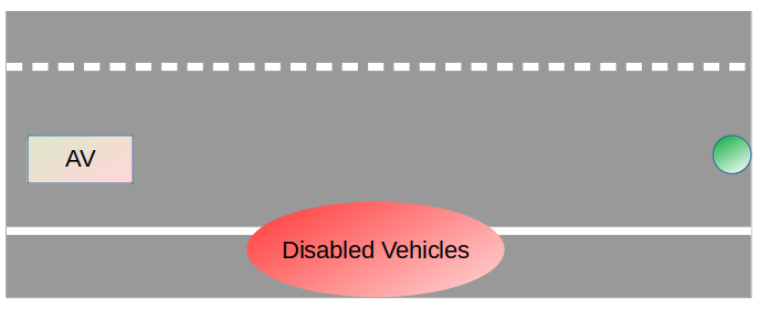
Figure 1: Road scenario

The assumption is that a breakdown is more likely in regions near the pair of disabled vehicles due to potential debris etc. which the AV must account for in navigating to the goal location indicated by the green dot; in this case, we assume the goal location and repair depot coincide. This increased likelihood of a breakdown is represented in the model by the function $\phi(x)$ given in Figure 2.

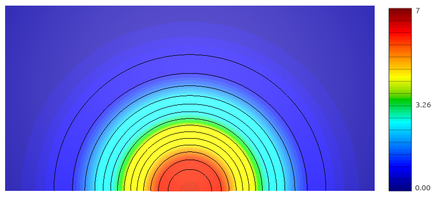
Figure 2: Counter plot of the spatially dependent likelihood of breakdown function $\phi(x)$ associated with the road layout in Figure 1.

For the above scenario we define $\Omega=[0,2]\times[0,1]$, let $G=D=(1.9,0.5)$, and uniformly refine a total of seven times. We set $f_{1}=1$, $f_{2}=0.2$, $R=1$, $K_{1}=1$, $K_{2}=1$ and define $\phi(x)=7e^{-5(x-1)^{2}-5*y^{2}}$ which is plotted above. Additionally, we take $\lambda=1$ and $\phi_{2}(x)=3$. Figures 3 and 4 display the contour plots associated with the value functions which correspond to vehicle operation in modes 1 and 2, respectively. A trajectory from any starting point $(x_{0},y_{0})$ is obtained by moving in the direction of the gradient. The contours show that the optimal trajectories move away from the disabled vehicles as expected.

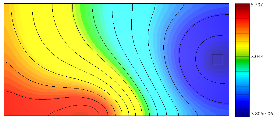
Figure 3: Value function $u_{1}$ corresponding to normal operation.

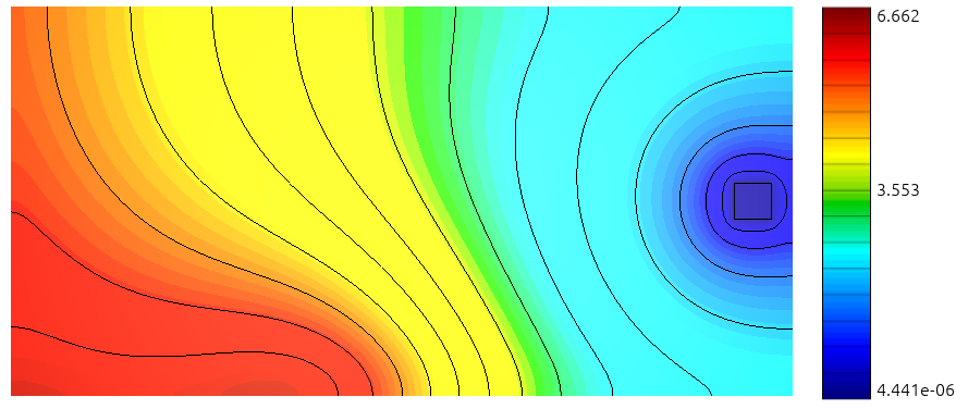
Figure 4: Value function $u_{2}$ which corresponds to operation after a partial breakdown.

VI Conclusions and future work

In this work, we considered the model of optimal path planning with random breakdowns introduced in [10] and analyzed from a theoretical point of view. We proved a comparison principle for viscosity solutions of the weakly coupled system of eikonal equations of the value functions. In particular, we described how to bypass the non-trivial degenerate coupling condition (5). Then we showed an example of how the lack of boundary conditions on the Aubry set can compromise the uniqueness of the solution. Finally, in the same example, we have provided boundary conditions for which the system does not have solutions. It still remains an open question how to choose boundary conditions to ensure the existence of a solution. Indeed, the few existence results proved for weakly coupled systems require that the coupling matrix is non-degenerate [19], or that the Aubry set is empty [37], or that the domain is a torus [14].

Future direction may also include the extension of the model in [10] to domains topologically more challenging, like networks, assuming not only that the vehicle is subject to breakdowns but also that the speed varies because of heterogeneous road conditions or the presence of lights at the nodes. Numerically, this work took advantage of finite element schemes used in convection-diffusion problems by iteratively solving a linearized form of the system augmented with artificial viscosity (10); specifically, the streamline diffusion approximation was used as a means of obtaining stable numerical solutions at each iteration. A number of schemes exist for such problems and the exploration of their utility in the context of the coupled system considered in this paper is one potential direction for future work.

References

- [1] P. Tompkins, Mission-directed path planning for planetary rover exploration. Carnegie Mellon University, 2005.
- [2] D. Nieto-Hernández, C.-F. Méndez-Barrios, J. Escareno, V. Ramírez-Rivera, L. Torres, and H. Méndez-Azúa, “Non-holonomic flight modeling and control of a tilt-rotor mav,” in 2019 6th International Conference on Control, Decision and Information Technologies (CoDIT), 2019, pp. 1947–1952.
- [3] A. Aguiar and A. Pascoal, “Regulation of a nonholonomic autonomous underwater vehicle with parametric modeling uncertainty using lyapunov functions,” in Proceedings of the 40th IEEE Conference on Decision and Control (Cat. No.01CH37228), vol. 5, 2001, pp. 4178–4183 vol.5.
- [4] J. Reeds and L. Shepp, “Optimal paths for a car that goes both forwards and backwards,” Pacific journal of mathematics, vol. 145, no. 2, pp. 367–393, 1990.
- [5] K. Alton and I. M. Mitchell, “Optimal path planning under different norms in continuous state spaces,” in Proceedings 2006 IEEE International Conference on Robotics and Automation, 2006. ICRA 2006. IEEE, 2006, pp. 866–872.
- [6] B. Chazelle, “Approximation and decomposition of shapes,” Algorithmic and Geometric Aspects of Robotics, vol. 1, pp. 145–185, 1985.
- [7] E. W. Dijkstra, “A note on two problems in connexion with graphs:(numerische mathematik, 1 (1959), p 269-271),” 1959.
- [8] L. E. Kavraki, P. Svestka, J.-C. Latombe, and M. H. Overmars, “Probabilistic roadmaps for path planning in high-dimensional configuration spaces,” IEEE Transactions on Robotics and Automation, vol. 12, no. 4, pp. 566–580, 1996.
- [9] S. LaValle, “Rapidly-exploring random trees: A new tool for path planning,” Research Report 9811, 1998.
- [10] M. Gee and A. Vladimirsky, “Optimal path-planning with random breakdowns,” IEEE Control Systems Letters, vol. 6, pp. 1658–1663, 2021.
- [11] H. T. Davis, Introduction to nonlinear differential and integral equations. US Atomic Energy Commission, 1960.
- [12] W. H. Fleming and H. M. Soner, Controlled Markov processes and viscosity solutions. Springer Science & Business Media, 2006, vol. 25.
- [13] M. H. Protter and H. F. Weinberger, Maximum principles in differential equations. Prentice Hall, Englewood Cliffs, 1967.
- [14] F. Camilli, O. Ley, P. Loreti, and V. D. Nguyen, “Large time behavior of weakly coupled systems of first-order hamilton–jacobi equations,” Nonlinear Differential Equations and Applications NoDEA, vol. 19, pp. 719–749, 2012.
- [15] F. Cagnetti, D. Gomes, and H. V. Tran, “Adjoint methods for obstacle problems and weakly coupled systems of pde,” ESAIM: Control, Optimisation and Calculus of Variations, vol. 19, no. 3, pp. 754–779, 2013.
- [16] H. Mitake and H. V. Tran, “Remarks on the large time behavior of viscosity solutions of quasi-monotone weakly coupled systems of hamilton–jacobi equations,” Asymptotic Analysis, vol. 77, no. 1-2, pp. 43–70, 2012.
- [17] H. Mitake, A. Siconolfi, H. V. Tran, and N. Yamada, “A lagrangian approach to weakly coupled hamilton–jacobi systems,” SIAM Journal on Mathematical Analysis, vol. 48, no. 2, pp. 821–846, 2016.
- [18] A. Davini and M. Zavidovique, “Aubry sets for weakly coupled systems of hamilton–jacobi equations,” SIAM Journal on Mathematical Analysis, vol. 46, no. 5, pp. 3361–3389, 2014.
- [19] H. Engler and S. M. Lenhart, “Viscosity solutions for weakly coupled systems of hamilton-jacobi equations,” Proceedings of the London Mathematical Society, vol. 3, no. 1, pp. 212–240, 1991.
- [20] H. Ishii and S. Koike, “Viscosity solutions for monotone systems of second–order elliptic pdes,” Communications in partial differential equations, vol. 16, no. 6-7, pp. 1095–1128, 1991.
- [21] M. Bardi and I. Capuzzo-Dolcetta, Optimal control and viscosity solutions of Hamilton-Jacobi-Bellman equations, ser. Systems & Control: Foundations & Applications. Birkhäuser Boston, Inc., Boston, MA, 1997, with appendices by Maurizio Falcone and Pierpaolo Soravia. [Online]. Available: https://doi.org/10.1007/978-0-8176-4755-1
- [22] J. A. Sethian, “A fast marching level set method for monotonically advancing fronts.” proceedings of the National Academy of Sciences, vol. 93, no. 4, pp. 1591–1595, 1996.
- [23] C.-Y. Kao, S. Osher, and Y.-H. Tsai, “Fast sweeping methods for static hamilton–jacobi equations,” SIAM journal on numerical analysis, vol. 42, no. 6, pp. 2612–2632, 2005.
- [24] A. Caboussat, R. Glowinski, and T.-W. Pan, “On the numerical solution of some eikonal equations: An elliptic solver approach,” Chinese Annals of Mathematics, Series B, vol. 36, no. 5, pp. 689–702, 2015.
- [25] Y. Yang, W. Hao, and Y.-T. Zhang, “A continuous finite element method with homotopy vanishing viscosity for solving the static eikonal equation,” Communications in Computational Physics, vol. 31, no. 5, pp. 1402–1433, 2022.
- [26] J.-L. Guermond, F. Marpeau, and B. Popov, “A fast algorithm for solving first-order pdes by l1-minimization,” Communications in Mathematical Sciences, vol. 6, no. 1, pp. 199–216, 2008.
- [27] D. Flad, A. Pradhan, and S. Murman, “Arbitrary order solutions for the eikonal equation using a discontinuous galerkin method,” arXiv preprint arXiv:2108.05950, 2021.
- [28] K. W. Morton, Revival: Numerical solution of convection-diffusion problems (1996). CRC Press, 2019.
- [29] E. Cartee, A. Farah, A. Nellis, J. Van Hook, and A. Vladimirsky, “Quantifying and managing uncertainty in piecewise-deterministic markov processes,” SIAM/ASA Journal on Uncertainty Quantification, vol. 11, no. 3, pp. 814–847, 2023.
- [30] M. G. Crandall, L. C. Evans, and P.-L. Lions, “Some properties of viscosity solutions of hamilton-jacobi equations,” Transactions of the American Mathematical Society, vol. 282, no. 2, pp. 487–502, 1984.
- [31] G. Namah and J.-M. Roquejoffre, “Remarks on the long time behavior of the solutions of hamilton-jacobi equations,” Communications in Partial Differential Equations, vol. 24, no. 5-6, pp. 883–893, 1999. [Online]. Available: https://doi.org/10.1080/03605309908821451
- [32] A. N. Brooks and T. J. R. Hughes, “Streamline upwind/Petrov-Galerkin formulations for convection dominated flows with particular emphasis on the incompressible Navier-Stokes equations,” Comput. Methods Appl. Mech. Engrg., vol. 32, no. 1-3, pp. 199–259, 1982, fENOMECH ”81, Part I (Stuttgart, 1981). [Online]. Available: https://doi.org/10.1016/0045-7825(82)90071-8
- [33] C. Johnson, Numerical solution of partial differential equations by the finite element method. Cambridge University Press, Cambridge, 1987.
- [34] R. E. Bank, P. S. Vassilevski, and L. T. Zikatanov, “Arbitrary dimension convection–diffusion schemes for space-time discretizations,” Journal of Computational and Applied Mathematics, vol. 310, pp. 19–31, 2017.
- [35] R. E. Bank and R. K. Smith, “An algebraic multilevel multigraph algorithm,” SIAM Journal on Scientific Computing, vol. 23, no. 5, pp. 1572–1592, 2002.
- [36] R. E. Bank. (2015) Multigraph 2.1. [Online]. Available: https://ccom.ucsd.edu/~reb/software.html
- [37] F. Camilli and P. Loreti, “Comparison results for a class of weakly coupled systems of eikonal equations,” Hokkaido Mathematical Journal, vol. 37, no. 2, pp. 349 – 362, 2008. [Online]. Available: https://doi.org/10.14492/hokmj/1253539559