SNR-Adaptive Ranging Waveform Design Based on
Ziv-Zakai Bound Optimization

Abstract

Location-awareness is essential in various wireless applications. The capability of performing precise ranging is substantial in achieving high-accuracy localization. Due to the notorious ambiguity phenomenon, optimal ranging waveforms should be adaptive to the signal-to-noise ratio (SNR). In this letter, we propose to use the Ziv-Zakai bound (ZZB) as the ranging performance metric, as well as an associated waveform design algorithm having theoretical guarantee of achieving the optimal ZZB at a given SNR. Numerical results suggest that, in stark contrast to the well-known high-SNR design philosophy, the detection probability of the ranging signal becomes more important than the resolution in the low-SNR regime.

I Introduction

Location information acquisition is one of the most indispensable sensing capabilities in wireless networks, which serves as a key enabler of a wide range of tasks including autonomous driving, internet of things, logistic and health care [1, 2, 3, 4]. Precise ranging is at the core of high-accuracy localization systems, for which waveform design is an essential task. Regarding ranging waveform design, a key observation is that the time-resolution of a ranging signal is roughly proportional to the reciprocal of its bandwidth, which has inspired many existing ranging techniques, including techniques based on ultra-wideband (UWB) signals [5, 6], as well as those benefitted from carrier aggregation [7, 8]. This insight has also given rise to considerable efforts devoted to network operation techniques yielding optimized bandwidth allocation strategies for localization systems [9, 10, 11].

From a theoretical perspective, the Cramér-Rao bound (CRB) of distance corroborates the “large bandwidth” intuition, stating that the lowest achievable mean-squared error (MSE) is inversely proportional to the squared root-mean-square (RMS) bandwidth [6]. In more precise terms, the RMS bandwidth is known to be proportional to the curvature of the signal autocorrelation function (ACF) at the peak [6]. As it can be observed from Fig. 1, when the signal-to-noise ratio (SNR) is high, the estimated distance (represented by $\hat{d}_{\rm H}$ in Fig. 1) would lie within the mainlobe around the true peak, and hence the ranging error is mainly determined by the aforementioned curvature. However, when the SNR is relatively low, there is a non-negligible probability that the maximum matched filter response locates at one of the ACF sidelobes, resulting in larger ranging errors corresponding to $\hat{d}_{\rm L}$ in Fig. 1. This issue is known as the “ambiguity phenomenon” [12], which suggests that the optimal ranging waveform should be SNR-adaptive.

Designing SNR-adaptive ranging waveforms would certainly rely on SNR-dependent performance metrics. CRB, being the most widely employed metric for estimators, does depend on SNR. Unfortunately, CRB is related to the ranging waveform only via its RMS bandwidth, suggesting that it does not account for the ambiguity phenomenon. Therefore, CRB-based waveform design yields a single waveform for any SNR. In fact, the actual MSE of the CRB-optimal waveform never attains the corresponding CRB (at an arbitrarily high SNR), as will be detailed later in this letter.

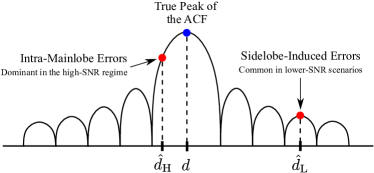
Figure 1: A sketchy illustration of the signal ACF and different types of ranging errors.

A promising candidate metric accounting for the ambiguity phenomenon is the Ziv-Zakai bound (ZZB) [13]. The main underlying idea of ZZB is that the MSE can be expressed in terms of the error probability of binary detection problems [14]. Intuitively, in the ranging problem, such binary detection problems concern distinguishing the true ACF peak from the sidelobes, and hence automatically take the ambiguity phenomenon into account. The ZZB of the ranging problem has been derived and analyzed extensively in the existing literature [13, 14, 15], showing that it does reflect the ambiguity issue in practice. However, to the best knowledge of the authors, ZZB has not been applied to waveform design, mainly due to its lack of closed-form expressions.

In this letter, instead of attempting to find suitable closed-form approximations, we aim for designing SNR-adaptive ranging waveforms by directly solving the ZZB optimization problem as a variational problem. Our contributions are summarized as follows.

• We show that the variational problem of ZZB optimization for ranging waveform design is a convex problem;

• We propose a discretized numerical reformulation of the ZZB optimization problem preserving the convexity, as well as an associated computation-efficient design algorithm based on the gradient projection method;

• Using numerical examples, we demonstrate that smaller RMS bandwidth can be more favorable under strong noise, suggesting that detection probability is preferred to resolution in the low-SNR regime.

Notations: Throughout the letter, we use $[\bm{x}]_{i}$ to represent the $i$-th entry of vector $\bm{x}$, and use $[\bm{A}]_{i,j}$ to represent the $(i,j)$-th entry of matrix $\bm{A}$.

II System Model

Let us consider the generic time-based ranging model of

$$y(t)=s(t-\tau)+n(t),$$ (1)

where $y(t)$ denotes the received signal, $s(t)$ represents the transmitted signal, $n(t)$ denotes the zero-mean white Gaussian noise having a constant power spectral density of $N_{0}$. The term $\tau=d/c$ denotes the propagation delay, with $c$ being the propagation speed (e.g. speed of light), and $d$ being the distance to be estimated. With this model in hand, we may obtain the following likelihood function

$$f(y;\tau) \propto e^{-\frac{1}{N_{\rm 0}}\int_{-\infty}^{\infty}(y(t)-s(t-\tau))^{2}{\rm d}t}$$

$$\propto e^{-\frac{2}{N_{\rm 0}}\left(R(\tau)+\int_{-\infty}^{\infty}n(t)s(t-\tau){\rm d}t\right)},$$ (2)

where $R(\tau)$ is the ACF of $s(t)$ given by $R(\tau)=\int_{-\infty}^{\infty}s(t-\tau)s(t){\rm d}t$.

According to [15], when the a priori distribution of the delay $\tau$ is a uniform distribution over $[\tau_{\min},\tau_{\max}]$, the ZZB of the distance $d$ takes the following form

$$\mathbb{E}\left\{(d\!-\!\hat{d})^{2}\right\} \!\geqslant\!\zeta_{\rm SNR}[\widetilde{R}]$$

$$: \!=\!\int_{0}^{\epsilon_{\max}}xQ\Big{(}\sqrt{2^{-1}{\rm SNR}(1\!-\!\widetilde{R}(x))}\Big{)}{\rm d}x,$$ (3)

where $\epsilon_{\max}$ is the maximum possible ranging error, namely $\epsilon_{\max}=c(\tau_{\max}-\tau_{\min})/2$, $Q(\cdot)$ denotes the function of $Q(z)=\int_{z}^{\infty}\frac{1}{\sqrt{2\pi}}e^{-\frac{1}{2}x^{2}}{\rm d}x$, $\widetilde{R}(x)$ denotes the normalized (and rescaled) ACF defined as

$$\widetilde{R}(x)=R(x/c)/R(0),$$ (4)

while ${\rm SNR}$ is the SNR given by ${\rm SNR}=\frac{1}{N_{0}}\int_{-\infty}^{\infty}s^{2}(t){\rm d}t$.

Remark 1

We are now in the position to illustrate a key difference between CRB-based waveform design and the proposed ZZB-based design. Specifically, the CRB of $d$ is given by [17]

$$\mathbb{E}\{(d-\hat{d})^{2}\}\geqslant c^{2}(8\pi^{2}\beta^{2}{\rm SNR})^{-1},$$ (5)

where $\beta=\int_{-\infty}^{\infty}f^{2}|S(f)|^{2}{\rm d}f/\int_{-\infty}^{\infty}|S(f)|^{2}{\rm d}f$ is the RMS bandwidth, with $S(f)$ being the Fourier transform of $s(t)$. In this expression, the term ${\rm SNR}^{-1}$ is merely a linear proportional factor. Consequently, the CRB-based optimal waveform does not vary with SNR. By contrast, observe that in the expression (II) of ZZB, ${\rm SNR}^{-1}$ no longer affects the ZZB in a simple linear manner, given the highly non-linear $Q$ function. Therefore, for different SNR values, the optimal signal ACF $\widetilde{R}(x)$ will be different. This enables us to design SNR-adaptive normalized ACFs.

III Problem Formulation and the Proposed Design Method

We consider the problem of SNR-adaptive waveform design under bandwidth constraint. In this letter, we consider the baseband ranging scenario, and assume that the fractional bandwidth is small. For a given design SNR ${\rm SNR}_{\rm D}$, this problem can be expressed as

$$\min_{\widetilde{R}(x)} \leavevmode\nobreak\ \leavevmode\nobreak\ \zeta_{{\rm SNR}_{\rm D}}[\widetilde{R}]$$ (6a)

$${\rm s.t.} \leavevmode\nobreak\ \leavevmode\nobreak\ \widetilde{R}(0)=1,\leavevmode\nobreak\ \widetilde{R}(x)\leqslant 1,\leavevmode\nobreak\ \forall x\in[0,\epsilon_{\max}].$$ (6b)

$$\leavevmode\nobreak\ \leavevmode\nobreak\ \int_{-\infty}^{\infty}\widetilde{R}(x)e^{-j\omega x}{\rm d}x\geqslant 0,\leavevmode\nobreak\ \forall\omega\in(-\infty,\infty),$$ (6c)

$$\leavevmode\nobreak\ \leavevmode\nobreak\ \int_{-\infty}^{\infty}\widetilde{R}(x)e^{-j\omega x}{\rm d}x=0,\leavevmode\nobreak\ \forall|\omega|>B,$$ (6d)

where (6c) follows from the positive semi-definiteness of ACFs, (6d) is the bandwidth constraint. In its original form, (6) is a variational problem which does not admit any analytical solution. Nevertheless, we have the following result:

Proposition 1 (Convexity of Variational ZZB Optimization)

The objective functional $\zeta_{\rm SNR_{D}}[\widetilde{R}]$ is a convex functional with respect to $\widetilde{R}(x)$.

Proof:

Please refer to Appendix A. ∎

Proposition 1 inspires us to find convex-preserving numerical reformulations of (6), which guarantee the achievability of the global optimum. In this letter, we consider the specific dicretized formulation as follows:

$$\min_{\bm{r}} \leavevmode\nobreak\ \leavevmode\nobreak\ \zeta_{{\rm SNR}_{\rm D}}(\bm{r}):=\sum_{i=1}^{N}x_{i}Q\left(\sqrt{2^{-1}{\rm SNR}_{\rm D}(1\!-\!r_{i})}\right)$$ (7a)

$${\rm s.t.} \leavevmode\nobreak\ \leavevmode\nobreak\ r_{1}=1,\leavevmode\nobreak\ \bm{r}\preccurlyeq\bm{1},\leavevmode\nobreak\ \bm{C}\bm{r}\succcurlyeq\bm{0},$$ (7b)

$$\leavevmode\nobreak\ \leavevmode\nobreak\ [\bm{C}\bm{r}]_{i}=0,\leavevmode\nobreak\ \forall i>B_{\rm dis},$$ (7c)

where (7c) is the discretized version of the bandwidth constraint, $N$ is the number of discretized sample points, $x_{i}=(i-1)\epsilon_{\max}/(N-1)$ denotes the $i$-th sample point, $\bm{r}=[r_{1},\dotsc,r_{N}]^{\rm T}$ is the sampled version of $\widetilde{R}(x)$, and $\bm{C}$ is the matrix of discrete cosine transform (DCT) satisfying

$$[\bm{C}]_{k,n}=\sqrt{\frac{2}{N}}\cos\left(\frac{\pi}{4N}(2k-1)(2n-1)\right).$$ (8)

Next, we show that this discretization is indeed convex-preserving.

Proposition 2

The problem (7) is convex.

Proof:

(Sketch) Computing the Hessian matrix of $\zeta_{{\rm SNR}_{\rm D}}(\bm{r})$ with respect to $\bm{r}$, and by noticing that $\frac{\partial^{2}\zeta_{{\rm SNR}_{\rm D}}(\bm{r})}{\partial r_{i}\partial r_{j}}=0$ holds for any $i\neq j$, we see that the Hessian matrix is positive semi-definite, and hence $\zeta_{{\rm SNR}_{\rm D}}(\bm{r})$ is convex. This further implies that the problem (7) is convex, since the feasible set characterized by (7b) and (7c) is a convex polytope. ∎

In light of Proposition 2, we can obtain the global optimal solution of (7) using the gradient projection method. The projection is practically implementable since the Hessian matrix is diagonal and can be readily calculated using (A). Specifically, the algorithm iterates as follows

$$\bm{u}^{(l)} ={\cal{P}}_{{\cal{S}}}\big{(}\bm{r}^{(l-1)}-\sigma\nabla\zeta_{{\rm SNR}_{\rm D}}(\bm{r}^{(l-1)})\big{)},$$ (9a)

$$\bm{r}^{(l)} =\bm{r}^{(l-1)}+\alpha_{l-1}(\bm{u}^{(l)}-\bm{r}^{(l-1)}),$$ (9b)

until convergence, where $\sigma$ is a fixed step size, while $\alpha_{l-1}$ is a variable step size satisfying the Armijo’s condition [19]. The projection operator ${\cal{P}}_{{\cal{S}}}(\bm{x})$ is defined by the following optimization problem

$${\cal{P}}_{{\cal{F}}}(\bm{x})=\mathop{\rm argmin}_{\bm{r}}\leavevmode\nobreak\ \|\bm{x}-\bm{r}\|^{2},\leavevmode\nobreak\ {\rm s.t.}\leavevmode\nobreak\ \bm{r}\in{\cal{S}},$$ (10)

where the feasible set ${\cal{S}}$ is given by

$${\cal{S}}=\left\{\bm{r}|r_{1}=1,\bm{r}\preccurlyeq\bm{1},\bm{C}\bm{r}\succcurlyeq\bm{0},[\bm{C}\bm{r}]_{i}=0,\forall i>B_{\rm dis}\right\}.$$

Although problem (10) can be solved by general-purpose convex optimization solvers (e.g. CVX [20]), such solvers may be computationally inefficient. To this end, we apply Dykstra’s projection method [21] to simplify the procedure. To elaborate, we compute ${\cal{P}}_{{\cal{S}}}(\bm{x})$ by iteratively applying the following rules

$$\bm{a}_{k} ={\cal{P}}_{{\cal{T}}}(\bm{x}_{k}+\bm{p}_{k}),\leavevmode\nobreak\ \bm{p}_{k+1}=\bm{x}_{k}+\bm{p}_{k}-\bm{a}_{k},$$ (11a)

$$\bm{x}_{k+1} ={\cal{P}}_{{\cal{F}}}(\bm{a}_{k}+\bm{q}_{k}),\leavevmode\nobreak\ \bm{q}_{k+1}=\bm{a}_{k}+\bm{q}_{k}-\bm{x}_{k+1},$$ (11b)

ensuring that $\bm{x}_{k}$ converges to ${\cal{P}}_{{\cal{S}}}(\bm{x})$ as $k$ increases, where the notations $\bm{p}_{k}$ and $\bm{q}_{k}$ are temporary intermediate variables, initialized by $\bm{p}_{0}=\bm{q}_{0}=\bm{0}$, $\bm{x}_{0}=\bm{x}$, the “temporal domain feasible set” ${\cal{T}}$ and the “frequency domain feasible set” ${\cal{F}}$ are defined as

$${\cal{T}} =\left\{\bm{r}|r_{1}=1,\bm{r}\preccurlyeq\bm{1}\right\},$$ (12a)

$${\cal{F}} =\left\{\bm{r}|\bm{C}\bm{r}\succcurlyeq\bm{0},[\bm{C}\bm{r}]_{i}=0,\forall i>B_{\rm dis}\right\},$$ (12b)

respectively. The corresponding projection operators are characterized by

$${[{\cal{P}}_{{\cal{T}}}(\bm{x})]}_{i} =\left\{\begin{array}[]{ll}1,&\hbox{$i=1$ or $i\neq 1,\leavevmode\nobreak\ r_{i}>1$;}\\ x_{i},&\hbox{otherwise,}\end{array}\right.$$ (13c)

$${[\bm{C}{\cal{P}}_{{\cal{F}}}(\bm{x})]}_{i} =\left\{\begin{array}[]{ll}0,&\hbox{$i>B_{\rm dis}$ or $[\bm{C}\bm{x}]_{i}<0$;}\\ {[\bm{C}\bm{x}]}_{i},&\hbox{otherwise.}\end{array}\right.$$ (13f)

Overall, the algorithm requires only $\rm SNR_{D}$, the fixed step size $\sigma$ and an initial guess $\bm{r}^{(0)}$ as inputs. The variable step sizes $\{\alpha_{l}\}$ can be determined at runtime. The workflow of the algorithm is summarized in Alg. 1.

Remark 2

Denoting the number of Dykstra’s iteration as $K$ (as used in Alg. 1), the complexity of our projection method is on the order of $O(KN\log N)$, by relying on fast DCT. By contrast, typical off-the-shelf solvers based on interior-point method would yield a complexity of $O(N^{3.5})$. This elucidates the computational efficiency of the proposed method.

Algorithm 1 The proposed waveform design algorithm.

1:  Initialize $\bm{r}^{(0)}$;

2:  for $l=1$:$L$ do

3:     Compute $\bm{x}_{0}=\bm{r}^{(l-1)}-\sigma\nabla\zeta_{{\rm SNR}_{\rm D}}(\bm{r}^{(l-1)})$;

4:     Initialize $\bm{p}_{0}=\bm{q}_{0}=\bm{0}$;

5:     for $k=1$:$K$ do

6:        $\bm{a}_{k}={\cal{P}}_{{\cal{T}}}(\bm{x}_{k}+\bm{p}_{k}),\leavevmode\nobreak\ \bm{p}_{k+1}=\bm{x}_{k}+\bm{p}_{k}-\bm{a}_{k}$;

7:        $\bm{x}_{k+1}={\cal{P}}_{{\cal{F}}}(\bm{a}_{k}+\bm{q}_{k}),\leavevmode\nobreak\ \bm{q}_{k+1}=\bm{a}_{k}+\bm{q}_{k}-\bm{x}_{k+1}$;

8:     end for;

9:     Let $\bm{u}^{(l)}=\bm{x}_{K}$;

10:     Compute $\bm{r}^{(l)}=\bm{r}^{(l-1)}+\alpha_{l-1}\left(\bm{u}^{(l)}-\bm{r}^{(l-1)}\right)$;

11:  end for;

IV Numerical Results

Throughout the numerical examples, we consider the scenario where $N=1000$, $B_{\rm dis}=40$. The initial guess $\bm{r}^{(0)}$ is set to be the Sinc pulse $\bm{s}$ satisfying

$$[\bm{C}\bm{s}]_{i}=\left\{\begin{array}[]{ll}c_{\rm s},&\hbox{$i\leqslant B_{\rm dis}$;}\\ 0,&\hbox{$i>B_{\rm dis}$,}\end{array}\right.$$ (14)

where $c_{\rm s}$ is a constant ensuring that $s_{i}=1$. We also use the Sinc pulse as a performance benchmark since it corresponds to a uniform frequency-domain power allocation strategy. We assume that both the transmitter and the receiver locate within the interval $[-1,1]$ on the real line, and thus the maximum distance estimation error is $\epsilon_{\max}=2$.

(a)

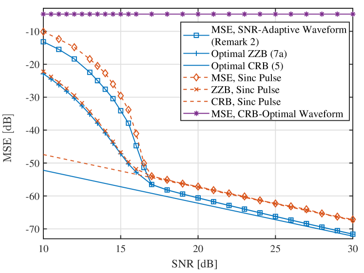
(b)

Figure 2: The MSE of the designed waveforms and benchmarks.

Before delving into details, we note that although the proposed algorithm designs the waveform that achieves the lowest ZZB at a given design SNR $\rm SNR_{D}$, the ZZB-optimal waveform at a specific $\rm SNR_{D}$ does not necessarily achieve the optimal MSE at that SNR, since ZZB is a only lower bound of the MSE. In light of this, we see that

Remark 3 (Adaptive Strategy)

We may conceive SNR-adaptive waveforms by selecting the ZZB-optimal waveform achieving the lowest MSE at each $\rm SNR_{D}$.

We first demonstrate the optimal ZZB achieved by the proposed method, portrayed in Fig. 2a. The first dotted line intersecting with the arrow in Fig. 2a represent ${\rm SNR}_{\rm D}=10$dB, the second denotes ${\rm SNR}_{\rm D}=13$dB, and so forth. The MSE achieved by certain ZZB-optimal waveforms at fixed $\rm SNR_{D}$, and that achieved using the adaptive strategy are also incorporated. Observe that the ZZB is achievable at relatively high SNR (i.e. larger than around $16$dB). Another noteworthy issue is that the ZZB-optimal waveform is indeed not necessarily MSE-optimal at ${\rm SNR}_{\rm D}$. For example, in Fig. 2a, the ZZB-optimal waveform at ${\rm SNR_{D}}=18$dB is not MSE-optimal until ${\rm SNR_{D}}=20$dB, while the ZZB-optimal waveform at ${\rm SNR_{D}}=13$dB is MSE-optimal around ${\rm SNR_{D}}=16.5$dB.

Next, let us compare the performance of the proposed SNR-adaptive waveforms with that of the Sinc pulse, as portrayed in Fig. 2b. Observe that the Sinc pulse achieves its corresponding CRB at relatively high SNRs. By contrast, the optimal ZZB does not attain the optimal CRB even at ${\rm SNR}=30$dB, but the gap between them shrinks as the SNR increases. Another closely-related phenomenon is that the MSE of the CRB-optimal waveform is unfavorable over the entire SNR range. To understand this phenomenon, first note that the CRB-optimal waveform $\bm{r}_{\rm CRB}$ is a sinusoidal signal, namely $[\bm{C}\bm{r}_{\rm CRB}]_{i}=1$ for $i=B_{\rm dis}$ and $[\bm{C}\bm{r}_{\rm CRB}]_{i}=0$ otherwise, according to (5). This waveform will never exhibit a CRB-achieving MSE at any SNR, since it is periodical and hence there will be unresolvable integer ambiguities resulting in uniformly distributed ranging errors across the entire region of interest, as can be observed from its poor MSE performance in Fig. 2b. In contrast to CRB, ZZB can reflect the ambiguity phenomenon. Consequently, the power spectral density of the ZZB-optimal waveform would have its mass more biased towards $B_{\rm dis}$ as the SNR increases, but will never become the impulse-like function corresponding to the CRB-optimal waveform, as portrayed in Fig. 3a. Therefore, despite that the ZZB-optimal waveforms do achieve their corresponding CRBs at high SNRs, the optimal CRB is not achievable for any finite SNR. As an ultimate limit, in the high-SNR regime, the minimum MSE is

$$\frac{1}{B}\Big{(}\int_{0}^{B}f^{2}B^{-1}{\rm d}f\Big{)}^{-1}=\frac{1}{3}$$ (15)

that of the MSE achieved by the Sinc pulse.

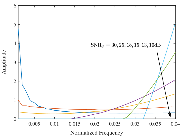
(a)

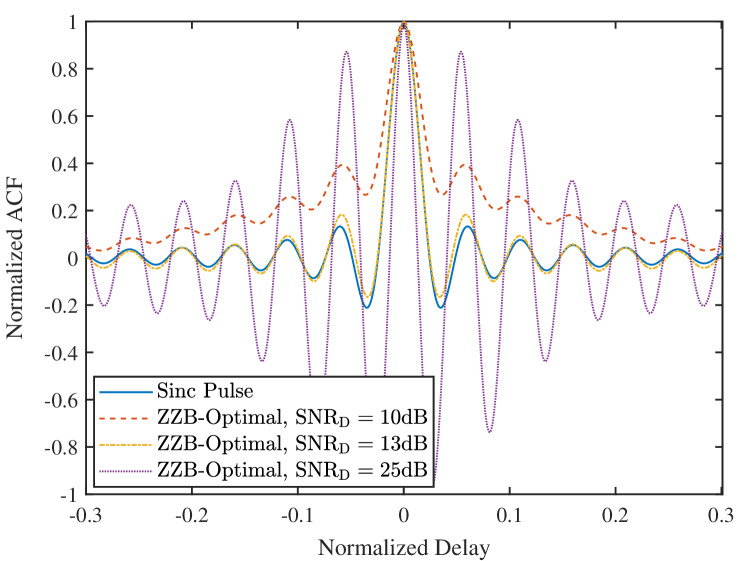
(b)

Figure 3: The frequency- and time-domain representations of the ZZB-optimal waveforms at various design SNRs.

We have seen that in the high-SNR regime, the RMS bandwidth is an important performance indicator, and provides a reasonable interpretation about the performance gain of the SNR-adaptive waveform over the Sinc pulse. However, similar arguments do not apply to the low-SNR regime. This can be seen from Fig. 3a, in which the RMS bandwidth of the waveform at ${\rm SNR_{D}}=10$dB is clearly smaller than that of the Sinc pulse, but it outperforms the Sinc pulse in the low-SNR regime ($\leqslant 15$dB), as can be observed from Fig. 2a and Fig. 2b.

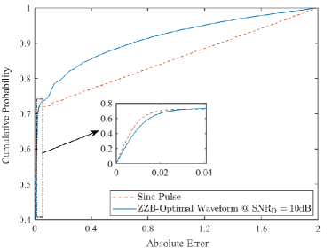
Figure 4: The cumulative distribution of absolute ranging error at ${\rm SNR}=10$dB, obtained by employing the Sinc pulse and the ZZB-optimal waveform at ${\rm SNR}_{\rm D}=10$dB, respectively.

To further understand the low-SNR performance, in Fig. 4, we plot the cumulative distribution function (CDF) of the absolute ranging error at ${\rm SNR}=10$dB obtained by the ZZB-optimal waveform at ${\rm SNR_{D}}=10$dB, and that of the Sinc pulse, respectively. Observe that when the cumulative probability is larger than $0.7$, the CDF of the Sinc pulse behaves similar to that of a uniform distribution, indicating that the Sinc pulse is essentially a “random guess” in this regime, clearly outperformed by the ZZB-optimal waveform. Interestingly, when the cumulative probability is less than $0.7$, the Sinc pulse outperforms the ZZB-optimal waveform (as seen in the zoomed-in figure). This phenomenon may be better illustrated by investigating the normalized ACFs $\widetilde{R}(x)$ shown in Fig. 3b. It is seen that the ACF mainlobe of the ZZB-optimal waveform at ${\rm SNR}_{\rm D}=10$dB is wider than that of the Sinc pulse, which explains why the Sinc pulse outperforms the ZZB-optimal waveform when the cumulative probability is less than $0.7$ (corresponding to the case in which the distance estimation still fall in the mainlobe). Nevertheless, outside the mainlobe, the ${\rm SNR}_{\rm D}=10$dB waveform still has a considerable autocorrelation, much larger than that of the Sinc pulse. Consequently, the Sinc pulse would find the signal completely lost in a strong noise, whereas the ${\rm SNR}_{\rm D}=10$dB waveform still preserves some ranging information, since its relatively large ACF values beyond the mainlobe would enhance the signal detection probability. This reveals a design philosophy compared in stark contrast to that in the high-SNR regime:

Remark 4

In the low-SNR regime, instead of improving the resolution, enhancing the detection probability is of the highest priority. This suggests that appropriately widening the ACF can be beneficial.

V Conclusions

In this letter, we have proposed a ranging waveform design method capable of adpating to the SNR, based on the ZZB. The proposed design method is guaranteed to yield the globally ZZB-optimal waveform due to the convexity of the formulated problem.

Beyond the design method, the numerical results suggest that the waveform design philosophy in the low-SNR regime is strikingly different from that in the high-SNR regime: Essentially, the main performance indicator is the time-resolution in the high-SNR regime, whereas the detection probability becomes more crucial in the low-SNR regime. Therefore, larger RMS bandwidth would be favorable for higher SNR, whereas smaller RMS bandwidth can be beneficial when the SNR is relatively low, which improves the detection probability at the cost of sacrificing some resolution. Possible applications of the proposed method include pulse shaping for target ranging, and power allocation for OFDM-based ranging systems.

Appendix A Proof of Proposition 1

Proof:

Note that for $x>0$, we have

$$Q(\sqrt{x})=\frac{1}{2\sqrt{\pi}}\Gamma\Big{(}\frac{1}{2},\frac{1}{2}x\Big{)},$$ (16)

where $\Gamma(s,t)$ denotes the incomplete Gamma function having the derivative of $\frac{\partial\Gamma(s,t)}{\partial t}=-t^{s-1}e^{-t}$ [22]. Also observe that the expression of $\zeta_{\rm SNR_{D}}[\widetilde{R}]$ does not contain the derivatives of $\widetilde{R}(x)$ with respect to $x$. Therefore, according to the Euler-Lagrange equation, the first-order variation of $\zeta_{\rm SNR_{D}}[\widetilde{R}]$ with respect to $\widetilde{R}$ is given by

$$\delta\zeta_{\rm SNR_{D}} =\int_{0}^{\epsilon_{\max}}\left[x\frac{{\rm d}}{{\rm d}\widetilde{R}}Q\left(\sqrt{2^{-1}{\rm SNR}_{\rm D}(1-\widetilde{R})}\right)\right]\delta\widetilde{R}{\rm d}x$$

$$=\frac{x{\rm SNR}_{\rm D}}{8\sqrt{\pi}}\int_{0}^{\epsilon_{\max}}\frac{e^{-\frac{\rm SNR_{D}}{4}(1-\widetilde{R})}}{\sqrt{\frac{\rm SNR_{D}}{2}(1-\widetilde{R})}}\cdot\delta\widetilde{R}{\rm d}x.$$ (17)

The second-order variation takes the following form

$$\delta^{2}\zeta_{\rm SNR_{D}} =\frac{x\sqrt{\rm SNR_{D}}}{4\sqrt{2\pi}}\int_{0}^{\epsilon_{\max}}e^{-\frac{\rm SNR_{D}}{4}(1-\widetilde{R})}(\delta\widetilde{R})^{2}$$

$$\hskip 8.53581pt\times\left(\frac{\rm SNR_{D}}{4}(1-\widetilde{R})^{\frac{1}{2}}+\frac{1}{2}(1-\widetilde{R})^{-\frac{3}{2}}\right){\rm d}x.$$ (18)

For $x\neq 0$, we have $1-\widetilde{R}(x)>0$. Thus for $x\in(0,\epsilon_{\max}]$, the second-order variation satisfies $\delta^{2}\zeta_{\rm SNR_{D}}>0$ for any $\delta\widetilde{R}$, implying that the functional $\zeta_{\rm SNR_{D}}[\widetilde{R}]$ is convex. ∎

References

- [1] M. Z. Win, Y. Shen, and W. Dai, “A theoretical foundation of network localization and navigation,” Proc. IEEE, vol. 106, no. 7, pp. 1136–1165, Jul. 2018.
- [2] Y. Xiong, N. Wu, Y. Shen, and M. Z. Win, “Cooperative localization in massive networks,” IEEE Trans. Inf. Theory, vol. 68, no. 2, pp. 1237–1258, Feb. 2022.
- [3] S. Kuutti, S. Fallah, K. Katsaros, M. Dianati, F. Mccullough, and A. Mouzakitis, “A survey of the state-of-the-art localization techniques and their potentials for autonomous vehicle applications,” IEEE Internet Things J., vol. 5, no. 2, pp. 829–846, Feb. 2018.
- [4] L. Chen et al., “Robustness, security and privacy in location-based services for future IoT: A survey,” IEEE Access, vol. 5, pp. 8956–8977, Apr. 2017.
- [5] S. Gezici et al., “Localization via ultra-wideband radios: A look at positioning aspects for future sensor networks,” IEEE Signal Process. Mag., vol. 22, no. 4, pp. 70–84, Jul. 2005.
- [6] Y. Shen and M. Z. Win, “Fundamental limits of wideband localization — part I: A general framework,” IEEE Trans. Inf. Theory, vol. 56, no. 10, pp. 4956–4980, Oct. 2010.
- [7] T. Kazaz, G. J. M. Janssen, J. Romme, and A.-J. van der Veen, “Delay estimation for ranging and localization using multiband channel state information,” IEEE Trans. Wireless Commun., vol. 21, no. 4, pp. 2591–2607, Apr. 2022.
- [8] M. Noschese, F. Babich, M. Comisso, and C. Marshall, “Multi-band time of arrival estimation for long term evolution (LTE) signals,” IEEE Trans. Mobile Comput., vol. 20, no. 12, p. 3383–3394, Dec. 2021.
- [9] M. Z. Win, W. Dai, Y. Shen, G. Chrisikos, and H. Vincent Poor, “Network operation strategies for efficient localization and navigation,” Proc. IEEE, vol. 106, no. 7, pp. 1224–1254, Jul. 2018.
- [10] T. Zhang, A. F. Molisch, Y. Shen, Q. Zhang, H. Feng, and M. Z. Win, “Joint power and bandwidth allocation in wireless cooperative localization networks,” IEEE Trans. Wireless Commun., vol. 15, no. 10, pp. 6527–6540, Oct. 2016.
- [11] T. Zhang, C. Qin, A. F. Molisch, and Q. Zhang, “Joint allocation of spectral and power resources for non-cooperative wireless localization networks,” IEEE Trans. Commun., vol. 64, no. 9, pp. 3733–3745, Sep. 2016.
- [12] S. Zafer, S. Gezici, and I. Guvenc, Ultra-wideband Positioning Systems: Theoretical Limits, Ranging Algorithms, and Protocols. Cambridge University Press, 2008.
- [13] D. Chazan, M. Zakai, and J. Ziv, “Improved lower bounds on signal parameter estimation,” IEEE Trans. Inf. Theory, vol. 21, no. 1, pp. 90–93, Jan. 1975.
- [14] K. Bell, Y. Steinberg, Y. Ephraim, and H. Van Trees, “Extended Ziv-Zakai lower bound for vector parameter estimation,” IEEE Trans. Inf. Theory, vol. 43, no. 2, pp. 624–637, Feb. 1997.
- [15] A. Mallat, S. Gezici, D. Dardari, C. Craeye, and L. Vandendorpe, “Statistics of the MLE and approximate upper and lower bounds — part I: Application to TOA estimation,” IEEE Trans. Signal Process., vol. 62, no. 21, pp. 5663–5676, Nov. 2014.
- [16] Y. Xiong, F. Liu, Y. Cui, W. Yuan, T. X. Han, and G. Caire, “On the fundamental tradeoff of integrated sensing and communications under Gaussian channels,” IEEE Trans. Inf. Theory, pp. 1–1, Early Access, 2023.
- [17] A. Liu, Z. Huang, M. Li, Y. Wan, W. Li, T. X. Han, C. Liu, R. Du, D. K. P. Tan, J. Lu, Y. Shen, F. Colone, and K. Chetty, “A survey on fundamental limits of integrated sensing and communication,” IEEE Commun. Surv. Tuts., vol. 24, no. 2, pp. 994–1034, 2nd Quart. 2022.
- [18] Y. Han, Y. Shen, X.-P. Zhang, M. Z. Win, and H. Meng, “Performance limits and geometric properties of array localization,” IEEE Trans. Inf. Theory, vol. 62, no. 2, pp. 1054–1075, Feb. 2016.
- [19] J. Nocedal and S. Wright, Numerical Optimization. Springer Science, 1999.
- [20] M. Grant and S. Boyd, “CVX: Matlab software for disciplined convex programming, version 2.1,” http://cvxr.com/cvx, Mar. 2014.
- [21] J. P. Boyle and R. L. Dykstra, “A method for finding projections onto the intersection of convex sets in hilbert spaces,” in Proc. Advances in Order Restricted Statistical Inference. New York, NY: Springer New York, 1986, pp. 28–47.
- [22] D. Zwillinger and A. Jeffrey, Table of integrals, series, and products, 7th ed. Elsevier, 2007.